| Issue |
A&A
Volume 674, June 2023
|
|
|---|---|---|
| Article Number | A93 | |
| Number of page(s) | 20 | |
| Section | Galactic structure, stellar clusters and populations | |
| DOI | https://doi.org/10.1051/0004-6361/202346095 | |
| Published online | 06 June 2023 | |
Ongoing hierarchical massive cluster assembly: The LISCA II structure in the Perseus complex
1
Department of Physics and Astronomy “Augusto Righi”, University of Bologna, via Gobetti 93/2, 40129 Bologna, Italy
2
INAF – Astrophysics and Space Science Observatory of Bologna, via Gobetti 93/3, 40129 Bologna, Italy
e-mail: This email address is being protected from spambots. You need JavaScript enabled to view it.
3
Department of Astronomy, Indiana University, Swain West, 727 E. 3rd Street, IN 47405 Bloomington, USA
4
INAF – Osservatorio Astrofisico di Arcetri, Largo Enrico Fermi 5, 50125 Florence, Italy
5
Institute for Astronomy, University of Edinburgh, Royal Observatory, Blackford Hill, Edinburgh EH9 3HJ, UK
Received:
7
February
2023
Accepted:
22
March
2023
Abstract
We report on the identification of a massive (∼105 M⊙) substructured stellar system in the Galactic Perseus complex likely undergoing hierarchical cluster assembly. This system comprises nine star clusters (including the well-known clusters NGC 654 and NGC 663) and an extended and low-density stellar halo. Gaia-DR3 and available spectroscopic data show that all its components are physically consistent in 6D phase-space (position, parallax, and 3D motion), and homogeneous in age (14–44 Myr) and chemical content (half-solar metallicity). In addition, the system’s global stellar density distribution is that of typical star clusters and shows clear evidence of mass segregation. We find that the hierarchical structure is mostly contracting toward the center with a speed of up to ≃4 − 5 km s−1, while the innermost regions expand at a lower rate (about ≃1 km s−1) and are dominated by random motions. Interestingly, this pattern is dominated by the kinematics of massive stars, while low-mass stars (M < 2 M⊙) are characterized by contraction across the entire cluster. Finally, the nine star clusters in the system are all characterized by a relatively flat velocity dispersion profile possibly resulting from ongoing interactions and tidal heating. We show that the observational results are generally consistent with those found in N-body simulations following the cluster violent relaxation phase, strongly suggesting that the system is a massive cluster in the early assembly stages. This is the second structure with these properties identified in our Galaxy and, following the nomenclature of our previous work, we named it LISCA II.
Key words: galaxies: star clusters: general / open clusters and associations: general / astrometry / stars: kinematics and dynamics / stars: formation
© The Authors 2023
 Open Access article, published by EDP Sciences, under the terms of the Creative Commons Attribution License (https://creativecommons.org/licenses/by/4.0), which permits unrestricted use, distribution, and reproduction in any medium, provided the original work is properly cited.
This article is published in open access under the Subscribe to Open model. This email address is being protected from spambots. You need JavaScript enabled to view it. to support open access publication.
1. Introduction
Cluster formation is important for the study of many key questions in modern astrophysics. First, it is central to the star formation process itself (e.g., McKee & Ostriker 2007). It is commonly accepted that most stars in galaxies (70%−90%) form in groups, clusters, or hierarchical systems, and spend some time gravitationally bound with their siblings when still embedded in their progenitor molecular cloud (Lada & Lada 2003). In the Milky Way (MW) this evidence comes from the global clustered structure of the disk and spiral arms (e.g., Kounkel & Covey 2019) and from the similar star formation rates observed in embedded clusters (Lada & Lada 2003) and in the field (Miller & Scalo 1979). On a larger scale, this indication is supported by the good agreement between the mass density in stellar clusters and the average co-moving stellar density at the peak of the universal star formation density at redshift ∼2 (Madau & Dickinson 2014).
Secondly, cluster formation has many implications for the early interplay between stellar and gas dynamics, the possible formation of gravitational wave sources (Di Carlo et al. 2019; Banerjee 2021), and the dynamical properties of young star clusters (e.g., McMillan et al. 2007; Ballone et al. 2020, 2021; Livernois et al. 2021; Tiongco et al. 2022). Finally, cluster formation is fundamental for our understanding of the assembly process of galaxies in a cosmological context, as major star-forming episodes in galaxies are typically accompanied by significant star cluster production (Forbes et al. 2018) and the main properties of these systems are thus strictly connected with those of their hosts (Brodie & Strader 2006; Dalessandro et al. 2012).
However, the possible presence of unifying principles governing the formation of stellar clusters and whether they form through a monolithic event or as a result of a hierarchical process of star formation in which stars are formed across a continuous distribution of gas densities is still a matter of debate (Lada et al. 1984; Moeckel & Bonnell 2009; Kruijssen 2012; Banerjee & Kroupa 2014, 2015; Treviño-Morales et al. 2019; Kuhn et al. 2019; Pang et al. 2022). In addition, the observed presence in the most massive clusters of the multiple stellar populations characterized by specific abundance patterns in a number of light elements (see, e.g., Bastian & Lardo 2018; Gratton et al. 2019 for recent reviews) has raised new questions on the physical mechanisms at the basis of cluster formation, and their dependence on the environment and the formation epoch (Krumholz et al. 2019). Despite the tremendous observational and theoretical efforts in the recent years (Allison et al. 2010; Parker 2014; Adamo et al. 2015), our understanding of how and where star clusters form is still in its infancy.
Numerous recent observational studies of stellar clusters have significantly enriched our knowledge about the properties of these systems. The unprecedented kinematical mapping of the Galaxy and its stellar components, as secured by the Gaia mission (Gaia Collaboration 2021), is revolutionizing the field (Cantat-Gaudin & Anders 2020; Cantat-Gaudin et al. 2020; Castro-Ginard et al. 2022; Cantat-Gaudin 2022) enabling detailed studies of nearby star-forming regions and their use as ideal laboratories to shed new light on our understanding of cluster formation and early evolution (e.g., Beccari et al. 2018; Meingast et al. 2019; Lim et al. 2020). Observations have revealed significant structural and kinematical complexity, such as significant deviations from spherical symmetry, the presence of extended tails in both young (e.g., Meingast et al. 2021; Jerabkova et al. 2021; Pang et al. 2021) and old star clusters (e.g., Grillmair 2019; Bonaca et al. 2020), as well as evidence of internal rotation and/or radially anisotropic velocity distributions (e.g., Hénault-Brunet et al. 2012; Ferraro et al. 2018; Kamann et al. 2018; Vasiliev & Baumgardt 2021; Dalessandro et al. 2021a).
It has also been shown that young stellar systems often have a complex clumpy structure characterized by the presence of several stellar subsystems (e.g., Kuhn et al. 2019, 2020; Getman et al. 2019; Lim et al. 2020; Dalessandro et al. 2021b; Zeidler et al. 2021). While some of these systems are likely to dissolve, some may evolve into massive and long-lived clusters. Interestingly in this context, Dalessandro et al. (2021b) have found that the well-known clusters h and χ Persei are just components of an association of clusters embedded in a wide stellar halo of similar age. This structure, named LISCA I (where LISCA stands for Lively Infancy of Star Clusters and Associations), has provided the first detailed observational picture of an ongoing massive cluster hierarchical assembly. This is the first time that such a formation mechanism has been identified in the MW and it has important implications on our understanding of the environmental conditions (both locally and in the distant Universe) necessary to form massive stellar clusters. For many years, hierarchical cluster formation was invoked as the preferred dynamical route to form rotating and high-ellipticity star clusters (e.g., de Oliveira et al. 1998). More recently, it has been used to interpret the properties of particularly massive and dynamically complex clusters (e.g., Lee et al. 1999; Brüns & Kroupa 2011), and as an avenue to form clusters with multiple populations with different light elements abundances (e.g., Gavagnin et al. 2016; Hong et al. 2017). However, while hierarchical cluster formation is believed to work efficiently in high-density starburst galaxies (e.g., Bastian et al. 2011; Chandar et al. 2011), we are still missing an adequate understanding of its effectiveness in lower density environments, like the MW and the Magellanic Clouds.
Dynamical simulations (Bonnell et al. 2003; Ballone et al. 2020; Livernois et al. 2021) show that within a hierarchical assembly framework, the fragmentation of a molecular cloud may lead first to the formation of tens of small clumps (∼100 M⊙). Then the surviving clumps merge to form a few more massive (103 − 104 M⊙) and larger clusters. Finally, one or two clusters survive this hierarchical merger process and will eventually evolve into a single massive cluster (e.g., Fujii & Portegies Zwart 2016; Livernois et al. 2021).
As a part of a larger project aimed at constraining the occurrence of the hierarchical assembly process within local disk-like galaxies, and at testing whether it is able to form long-lived systems surviving the initial and turbulent few tens of million years of existence (e.g., Moeckel & Bate 2010; Gieles et al. 2006), we present a detailed photometric and kinematic study, mainly based on Gaia DR3 data (Gaia Collaboration 2023), of a region in the Galactic Perseus Arm including the clusters NGC 663 and NGC 654, that appears to be analogous to LISCA I. We also present a comparison of the observational results with the dynamical properties emerging in N-body models following the violent relaxation phase of a stellar system and its subsequent evolution.
The paper is structured as follows. The adopted data set is presented in Sect. 2. Sections 3 and 4 describe the physical properties of the area under study, its structure and kinematics, respectively. Section 5 presents the physical properties of star clusters belonging to the system. In Sect. 6 we discuss the total system’s mass. A comparison with a set of N-body simulations is described in Sect. 7. The main conclusions are drawn in Sect. 8.
2. Catalogs and preliminary analyses
2.1. The catalogs
From the Gaia Archive1 we retrieved DR3 data for sources distributed within a large area on the sky (5° in radius) arbitrarily centered on the position of NGC 654 and having a five-parameter astrometric solution (i.e., sources with sky position, proper motion, and parallax measurements) and G < 19.5 mag. This catalog comprised 4.5 million sources.
We supplemented this data set with high-resolution optical and near-infrared spectra obtained with the HARPS-N (Cosentino et al. 2014) and GIANO-B (Oliva et al. 2012; Tozzi et al. 2016) spectrographs at the TNG as part of the SPA - Stellar Population Astrophysics: the detailed, age-resolved chemistry of the Milky Way disk Large Program (Program ID A37TAC13, PI: L. Origlia). Line-of-sight (LOS) velocities were obtained for all the observed stars, while detailed chemical abundances for the subsample of red supergiants were computed by Fanelli et al. (2022).
2.2. Clustering analysis
As any coherent stellar structure in the considered area should appear as an overdensity in the multi-dimensional phase-space of positions and velocities, we performed a clustering analysis on the whole catalog by means of the Hierarchical Density-Based Spatial Clustering of Application with Noise (HDBSCAN) algorithm (McInnes et al. 2017). For each star we used as inputs the Galactic coordinates, parallax, and proper motion components (ℓ,b, ϖ, μα*, μδ), and we set the HDBSCAN parameters as min_cluster_size = 40 and min_samples = 30. The parameter min_cluster_size sets a lower limit to the number of objects an overdensity should have to be identified as a cluster (hence we could not identify clusters with fewer than 40 members), while min_samples represents the number of sources used in determining the nearest neighbor distance for each source. Hence, increasing min_samples increases the mutual reachability distance among sources, and only the densest areas survive as clusters2. Furthermore, HDBSCAN assigns a cluster membership probability to each star based on its distance from the neighboring stars. The closer the star is to the other cluster members, the higher the membership probability, and vice versa.
We identified 131 clustered systems within the full 5° field of view. To exclude spurious detections and select only systems that can be classified as clusters to a high significance level, we followed the post-processing approach described by Hunt & Reffert (2021), which uses the nearest-neighbors distance as a proxy for the local density. Only structures with a median value of the nearest-neighbors distance smaller than that of field stars at a 3σ level according to a Mann-Whitney statistics (Mann & Whitney 1947) were flagged as true stellar clusters. Out of 131 putative clusters, 54 systems fulfilled these criteria and were retained for the subsequent analysis. Recent open clusters catalogs (e.g., Cantat-Gaudin & Anders 2020; Cantat-Gaudin et al. 2020; Castro-Ginard et al. 2022) list 45 clusters in the region with more than 40 members (which is our threshold for identification). Interestingly, we recovered all the known clusters but two (hence 11 unknown structures were identified by this study), namely UBC 186 and UPK 265. We verified that UPK 265 could have been recovered by slightly changing the input parameters we set for the clustering analysis; however, it would have been excluded by the preliminary parallax selection (according to its value reported by Cantat-Gaudin et al. 2020) described below. The case of UBC 186 is more interesting. A careful investigation of its members reveals significant overlap with NGC 581 (128 out of 131 of NGC 581 members are in common with UBC 186; Cantat-Gaudin et al. 2020). Our analysis was able to properly identify both NGC 581 and another nearby structure that was labeled as UBC 186 by Cantat-Gaudin et al. (2020). However, the latter was flagged as a false detection by the adopted post-processing routine. It is important to note here, however, that the following analysis and the results of this paper do not depend on the inclusion or exclusion of any specific substructure or cluster.
Starting from the sample of 54 structures, we performed a preliminary selection to identify clusters sharing 3D position and 2D velocity with NGC 654 (ϖ = 0.31 ± 0.05 mas, μα* = −1.1 ± 0.1 mas yr−1 and μδ = −0.3 ± 0.1 mas yr−1, obtained by Cantat-Gaudin et al. 2020, using Gaia DR2 data), retaining only those with distance D = 2.8 − 3.2 kpc and co-moving within about 5.5 km s−1 (corresponding to 0.38 mas yr−1 at 3 kpc), according to their median parallax and proper motion estimated from Gaia DR3 data. Nine clusters (comprising NGC 654 itself) were selected in this way. We note in passing that none of the 11 previously unknown structures fulfilled these criteria.
Finally, we determined physically motivated selections in parallax and proper motion with the aim of selecting all the sources in the field of view sharing 3D position and 2D velocity with the nine clusters. Specifically, we inferred the intrinsic cluster distributions in parallax and proper motion (by using only stars with membership probability higher than 90%) by means of a Gaussian mixture modeling technique (the Extreme Deconvolution3 package developed by Bovy et al. 2011), thereby properly accounting for errors and correlation between measurements. In Fig. 1 we show the distributions inferred in this way in the parallax (top panel) and proper motion components (bottom panel).
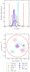 |
Fig. 1. Inferred distributions in parallax (top panel) and proper motion (bottom panel) from likely (> 90%) cluster members. Different stellar clusters are in different colors. Dashed gray lines in the bottom panel are iso-probability contours at the 1, 2, and 3σ levels. The red dashed circle and vertical lines represent the range in proper motion and parallax inside which stars were selected. |
We thus retained all the sources in the Gaia catalog with proper motions and parallaxes compatible, within 3σ, to the cluster distribution. Selected stars share similar distances, ϖ ∈ [0.285; 0.407] mas, which corresponds to D ∈ [2.46; 3.51] kpc, and co-move within 0.536 mas yr−1 (about 7.5 km s−1). In Fig. 2 we show the 2D density map of the region along with iso-density contours. The iso-density curves highlight the presence of small-scale clumpy structures corresponding to the identified stellar clusters (labeled in blue) as well as a lower-density diffuse halo extending for at least 3° from NGC 663 and NGC 654 and co-moving with the clusters.
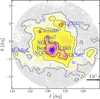 |
Fig. 2. Spatial distribution in Galactic coordinates of stars selected in proper motion and parallax. Star cluster names are shown in blue, while black lines are iso-density contours enclosing 11.8% (solid), 39.3% (dashed), and 67.5% (dash-dotted) of the normalized star density distribution. The black arrow shows the direction of the Galactic center (GC). |
2.3. Completeness of the Gaia catalog
The estimate of the Gaia catalog completeness is certainly a challenge due to, for instance, a composite data reduction pipeline and a complex satellite scanning law. Moreover, it does not depend only on the telescope properties themselves, but also on the physical properties of the observed regions such as crowding and extinction. This issue was first tackled by Everall et al. (2021, for the DR2) and Everall & Boubert (2022, for the EDR3) who directly modeled Gaia’s reduction pipeline and scanning law. More recently, Cantat-Gaudin et al. (2023) adopted an empirical approach to estimate the photometric completeness in the G band by comparing the Gaia catalog with the Dark Energy Camera Plane Survey (Schlafly et al. 2018; Saydjari et al. 2023).
For the purpose of this study, we need to assess the probability that a source is included in the catalog with magnitude G measure and a five-parameter solution. The resulting joint probability is
 (1)
(1)
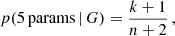
We retrieved the first term on the right-hand side from the completeness maps of Cantat-Gaudin et al. (2023) (see Fig. 3 for the 2D map of photometric completeness computed for G = 19.5 mag), whereas the p(5 params | G) term in Eq. (1) was estimated from the number count ratios between sources with the five-parameter solution (k) compared to the total number of sources (n) for a given sky patch and magnitude bin
 (2)
(2)
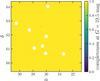 |
Fig. 3. Two-dimensional map of the p(G) term in Eq. (1) for G = 19.5 mag, computed with the GaiaUnlimited package (Cantat-Gaudin et al. 2023). White points show the location of star clusters. |
following the documentation of the GaiaUnlimited project4. We computed Eq. (2) for a regular spatial grid in a region of 10° around NGC 654 assuming a spatial bin size of Δδ = 0.2° (thus it follows Δα = Δδ cos δNGC654 ≃ 0.42° in order to obtain a square grid) and for magnitude bins of ΔG = 0.2 mag down to G ≤ 19.5 mag.
In Fig. 4 we show as examples the 2D p(5params | G) maps computed for G = 18.5 mag (left panel) and G = 19.5 mag (right panel).
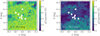 |
Fig. 4. Catalog completeness in the five-parameter solution estimated from star count ratios (p(5params|G) term in Eq. (2)) for G = 18.5 mag (left panel) and G = 19.5 mag (right panel). White points give the positions of star clusters. |
The comparison between Figs. 3 and 4 clearly shows that the selection of sources with the five-parameter solution has a dominant impact on the final completeness. Indeed, p(5params | G) significantly drops for G > 18.5 mag, while p(G) remains almost equal to 1 down to G = 19.5 mag. Hence, in the following we assumed p(G) = 1, and thus simplifying Eq. (1) and Eq. (2) into:
 (3)
(3)
In the subsequent analyses we correct stellar counts for incompleteness according to Eq. (3).
3. Physical properties of the observed area
In Sect. 2.2 we identified a region encompassing nine star clusters embedded in a low-density and diffuse stellar halo (see Fig. 2) lying within strict ranges in 2D velocity, position, and parallax by construction. In this section we characterize the physical properties of the area based on the Gaia photometry and the spectroscopic data.
3.1. Differential reddening
Available Galactic extinction maps (e.g., Schlegel et al. 1998 and recalculations from Schlafly & Finkbeiner 2011) report a quite significant and strongly variable (E(B − V)∼0.5 − 3.5 mag) extinction along the LOS for the region under investigation. Here we provide an independent estimate of the differential reddening based on a suitable color-color diagram and following the approach adopted by Dalessandro et al. (2018). In particular, combining the Gaia G band with the r, i, z photometric bands from the Panoramic Survey Telescope and Rapid Response System (Pan-STARRS data release 2, Chambers et al. 2016), we constructed the (G − r) versus (i − z) color-color diagram. This diagram turned out to be the most suitable choice as the evolutionary sequences run almost orthogonally to the reddening vector in these colors.
We derived differential extinction star by star by minimizing differences along the reddening vector with respect to a reference system. As a reference, we chose the median color-color distribution of likely main sequence stars (G > 12 mag or GBP − GRP < 0.5 mag) belonging to the cluster NGC 581. NGC 581 stars are distributed on average at bluer colors than other stars in the field, thus suggesting they are located in a region with relatively small extinction (color excess for these stars was derived from Schlegel et al. 1998; Schlafly & Finkbeiner 2011: E(B − V)NGC581 ≃ 0.54 mag). Afterward, for each star, we obtained the median colors of the closest 50 likely main sequence (G > 12 mag or GBP − GRP < 0.5 mag) neighbor stars, and we determined the distance of this median value to the reference point along the reddening vector (using coefficients from Cardelli et al. 1989). The extinction value corresponding to the derived distance is then assigned to the specific star. To all the sources that do not fulfill the criteria of being likely main sequence stars and to those that do not have a counterpart in the PanSTARRS catalog, we assign the median reddening of the closest 50 neighbors.
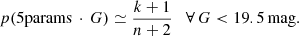
As a representative example, we show in Fig. 5 the observed CMD of NGC 663 members as well as those obtained using extinction values from Schlafly & Finkbeiner (2011) (in red) and obtained in this work (in blue). The differential reddening corrections derived in this work nicely squeeze the sequence in the CMD compared to the observed one, and thus confirm the robustness of our estimates. On the contrary, those from Schlafly & Finkbeiner (2011) significantly spread the sequence and move stars at nonphysical colors, reaching (GBP − GRP)0 = −2 mag, thus suggesting that the adopted values for the E(B − V) variations are likely overestimated.
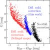 |
Fig. 5. Color-magnitude diagram for NGC 663 members. In black the observed photometry, while in red and blue are shown the distributions of stars after correcting for differential reddening. For the former Galactic extinction maps by Schlegel et al. (1998), Schlafly & Finkbeiner (2011) are used, and for the latter the reddening corrections estimated in this work. |
Finally, in Fig. 6 we show the resulting reddening map, as derived in this work, in which each star in the catalog is color-coded according to the inferred extinction. We note here that while differential reddening might play a role in shaping specific features of the iso-density contours shown in Fig. 2 (i.e., missing sources due to locally higher extinction artificially produces underdense regions), it is unlikely that it impacts the overall observed density gradient across the field of view as low-extinction regions, such as b ≲ −3° (see Fig. 6), still result as underdense compared to the diffuse halo. In Fig. 7 we show the observed (left panel) and differential reddening corrected (right panel) CMDs of the full catalog for comparison.
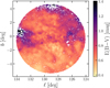 |
Fig. 6. Two-dimensional reddening map in Galactic coordinates. The extinction was computed star by star from color-color diagrams (see text for further details). White areas correspond to regions devoid of stars. |
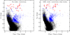 |
Fig. 7. Observed (left panel) and differential reddening corrected (right panel) CMD for the full catalog. In blue we show stars with LOS velocity measurements from Gaia DR3 (big squares for stars considered in the LOS analysis), whereas in red are stars targeted by high-resolution spectroscopy. The subsample with chemical abundances is circled in red. |
3.2. Cluster and halo ages
Determining the ages of young (< 100 Myr) sparsely populated star clusters is certainly a challenge. At these ages, the color-magnitude distribution of turn-off stars is strongly affected by stellar rotation (Li et al. 2019). Moreover, the low number of stars and short evolutionary timescales of massive stars (> 10 M⊙) might hamper a detailed estimate of the bright and blue main sequence termination, which in turn would bias the age inferred by standard methods such as isochrone fitting. Notwithstanding these limitations, here we attempt to tackle this issue by adopting a specific approach that is only marginally sensitive to stellar rotation and minimizes the impact of low-number statistics. In particular, we used a set of synthetic simple stellar populations obtained from the PARSEC database (Bressan et al. 2012) with [Fe/H] ≃ (−0.30 ± 0.01) dex (corresponding to the mean metallicity of the area Fanelli et al. 2022) and sampling the age range 1–100 Myr with a regular step of 1 Myr. We compared them with the observed cumulative luminosity functions (CLFs) in the G band, after correcting for differential reddening5 and completeness, as described in Sect. 2.3.
In order to account for number fluctuations, we randomly picked several times (≃100) a (virtually) independent sample of N stars from each synthetic population. The number of extracted stars N was set to be the number of objects in the synthetic population with G0 > 6 mag after applying a normalization to the luminosity function in the range 12.5 < G0 < 16 mag (at least 2 mag fainter than the main sequence termination for populations younger than 100 Myr at a distance of about 3 kpc). For each extraction, we then constructed the CLF, and we determined the median CLF of all the extractions (as well as its corresponding 68% credible region). The median CLF obtained for different ages was then compared to the observed one (see, e.g., Fig. 8) and the best fit was defined as the one that minimizes the χ2 statistics. Comparison with the CLF was carried out up to G = 18 mag (corresponding to about G0 ≃ 16 mag), below which the catalog’s completeness drops (see Fig. 4).
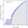 |
Fig. 8. Cumulative luminosity function for the stellar cluster NGC 654 (gray histogram), along with the normalized histogram of a 32 Myr old synthetic population computed with the PARSEC model (blue histogram). The error bars show the standard deviation of the model’s count fluctuations due to several extractions (see text for further details). Bins are 0.5 mag wide. |
Furthermore, when comparing the synthetic CLF to the observed one, we looked for supergiant stars in the range G0 < 8 mag and (GBP − GRP)0 > 0.2 mag. If present, these stars provide strong constraints on the age, and hence we limited the analysis only to those ages that are able to explain the presence of evolved stars at the observed magnitudes. This allowed us to inform the fitting procedure about the likely young age of the system, even in absence of bright, blue main sequence stars. We note that with this procedure we assigned a narrower uniform prior to the cluster’s age. If red supergiants were not present we did not apply any selection on the age.
Color-magnitude diagrams for each cluster are shown in Fig. 9 along with best-fit isochrones. The nine clusters have ages in a narrow range of 14 − 44 Myr. The only exception is Berkeley 6, for which we derived an age of  Myr. We also found a slight mismatch between isochrones and data, especially visible in the clusters Riddle 4 and NGC 654. This discrepancy likely results from local underestimations of the differential reddening, which in turn biases the age inference toward older ages.
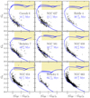 |
Fig. 9. Color-magnitude diagrams of cluster members (black dots) corrected for differential reddening. For each cluster, the best-fit isochrone is shown in blue and the median age along with the 68% credible interval is also reported. The shaded areas show the region inside which stars are flagged as supergiants. |
Nevertheless, typical errors in age estimates are about 10 − 15 Myr (Fig. 9). They account only for uncertainties arising from the fitting procedure, although errors in the differential reddening, distance, and incorrect membership assignment might also be important sources of uncertainties. However, we note that we are mainly interested in constraining relative ages rather than absolute ones.
A comparison with ages from the literature shows qualitatively overall agreement as they are in the range 15 − 38 Myr for the clusters under study (Cantat-Gaudin et al. 2020). The only exception is Berkeley 6 for which Cantat-Gaudin et al. (2020) report an age of about 200 Myr, consistent with the system being older than other clusters.
Finally, the same analysis was carried out for the stellar halo (i.e., all the stars that did not belong to any cluster according to the membership probabilities assigned by the clustering algorithm), finding that its age ( Myr) is consistent with the ages of the clusters embedded within it.
3.3. Line-of-sight velocity distribution and iron content
We investigated the LOS velocity and the metallicity distributions in the region using the TNG-GIARPS spectroscopic catalog presented in Sect. 2.1 (shown in red in Fig. 7), and we compared them with those expected for the surrounding Galactic field obtained from the Besançon Milky Way model (Robin et al. 2003) after applying the same parallax and proper motion selections. We computed LOS velocities for 24 stars, five of which are cluster members, while the remaining 19 belong to the halo. Among them, chemical abundances are available for the seven red supergiants (double red circles in Fig. 7), one of which belongs to NGC 581.
We also note that, while Gaia DR3 (Gaia Collaboration 2023) provides LOS velocity for 1164 selected stars, their color-magnitude distribution (shown in Fig. 7) suggests they are mostly field interlopers. Nevertheless, some bright stars that are likely members of the system have LOS measurements from Gaia. We therefore selected those stars with G0 < 8 mag (removing objects belonging to the older disk population) and with rv_expected_sig_to_noise> 5 and rv_renormalised_gof< 2 (thus selecting sources with reliable LOS velocity; see Katz et al. 2019). Out of the 1164 stars, only 4 fulfilled these criteria and were thus included in the catalog (shown as larger blue squares in Fig. 7).
In Fig. 10 we show the distributions in LOS velocity (left panel, constructed with 24 stars from the high-resolution spectroscopic catalog plus 4 stars from Gaia DR3) and in [Fe/H] abundance (right panel, for the seven red supergiants), superimposed to the distributions of the surrounding Galactic field. The intrinsic widths of the observed distributions were inferred by means of a maximum likelihood approach (accounting for individual errors on measurements), and in Fig. 10 we report their median values along with the 68% credible intervals. In particular, we obtained a LOS velocity dispersion  km s−1 (to be compared with σLOS, MW = 20 km s−1) and a mean velocity
 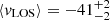 km s−1, whereas for the metallicity we obtained a dispersion
 ![Mathematical equation: $ \sigma_{[\mathrm{Fe}/\mathrm{H}]}=0.008^{+0.009}_{-0.005} $](/articles/aa/full_html/2023/06/aa46095-23/aa46095-23-eq8.gif) dex (opposed to σ[Fe/H] = 0.2 dex for the Galactic field) and a mean metallicity
dex (opposed to σ[Fe/H] = 0.2 dex for the Galactic field) and a mean metallicity ![Mathematical equation: $ \langle [\mathrm{Fe}/\mathrm{H}]\rangle=-0.30^{+0.01}_{-0.01} $](/articles/aa/full_html/2023/06/aa46095-23/aa46095-23-eq9.gif) dex.
dex.
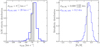 |
Fig. 10. LOS velocity (left panel) and iron-over-hydrogen abundance (right panel) distributions for members of the selected structure (gray histogram) and for a Milky Way model (blue histogram). The intrinsic dispersions are also shown in the top left corners. All the distributions are scaled by a constant factor for visualization purposes only. |
Interestingly, the observed distributions of the stars in the region are significantly narrower than those expected for a randomly selected group of co-moving Galactic stars, thus strengthening the evidence of kinematic coherence and suggesting a significant chemical homogeneity. In addition, the consistency in both LOS velocity and chemical content between cluster and halo stars further validates the assumption of a physical and coherent structure embedding the star clusters.
The literature data on the bulk clusters’ LOS velocity support the kinematic coherence of all clusters but one. The LOS velocity reported for Berkeley 6 (vLOS ≃ −89 ± 52 km s−1, Tarricq et al. 2021) is significantly lower than the system’s bulk velocity. However, we note that this value is still compatible within the huge uncertainty as only two stars were used for its estimate. Moreover, Spina et al. (2021) measured the iron content for one member of Berkeley 6 to be around [Fe/H] ∼ − 0.179 dex, significantly higher than [Fe/H] ≃ − 0.3 dex, although we note again that chemical abundances were derived for only one cluster member whose membership probability is < 30% (Spina et al. 2021). Therefore, better constraints on the stellar membership, age, and 3D velocity are needed before drawing any conclusions about the role of Berkeley 6 in the system.
4. Structural and kinematic properties of the diffuse stellar halo
4.1. Density distribution
We constructed the number density profile of the diffuse stellar halo. We took as the system’s center the center of mass of stars with M ≥ 2 M⊙. First, celestial coordinates were converted into local Cartesian ones, assuming the centroid of the system as an initial guess for the system’s center. After that, the center of mass was computed in Cartesian coordinates and it was converted back into celestial coordinates, obtaining (αCM; δCM) = (26.4559; 61.7865) degree.
We binned stars radially with respect to this center and we set the width of each radial annulus to contain 2500 sources each. Radial shells were then split into four angular sectors where the density was computed simply as the ratio of the number of stars to the sector’s area. The final shell density and error were the mean and standard deviation of the four measurements, respectively. Finally, we also accounted for Poissonian error in each bin by summing in quadrature to the standard deviation a term  , with Nshell being the number of stars within the shell.
In Fig. 11 we show the number density profile for sources out to 8° from the system’s center of mass and with G ≤ 18 mag. When studying the density distribution, we temporarily extended the catalog up to 8° from the system’s center in order to assess the background density, while the selection in G was a good compromise between the catalog’s completeness and statistics. Interestingly, the observed density resembled a cluster-like profile over about a factor of 10 in density. At about R ≳ 6°, the density profile flattens, and we estimated the background density as the weighted mean of bins at distances larger than 6° from the adopted center, obtaining Σ⋆,background ≃ 1.5 × 10⁻⁵ stars arcsec−2, which was then subtracted from the observed profile.
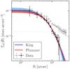 |
Fig. 11. Stellar number density profile of an 8° region around the system’s center of mass and considering stars brighter than G = 18 mag. The observed profile is shown in gray, while the intrinsic profile (after background subtraction) is shown in black. The Plummer model (in red) and the King model (in blue) are also shown, along with the corresponding 68% credible regions constructed from the posterior samples. |
Finally, we fitted the density distribution within 5° using the King (King 1962) and Plummer (Plummer 1911) models, which are typically adopted to reproduce stellar cluster density profiles. All the free parameters were constrained assuming a χ2 likelihood and uniform priors (in logarithm), and exploring the parameter space with a Markov chain Monte Carlo (MCMC) technique using the Python package emcee6 (Foreman-Mackey et al. 2013).
In Fig. 11 we therefore show the density profile (before the background subtraction in gray, and after in black) along with the best-fit models and the associated errors. Both models provided a nice description of the data.
4.2. Kinematic properties
We investigated the kinematic properties of the stellar halo by further selecting stars fulfilling the following astrometric quality selection criteria (Lindegren et al. 2021): ruwe ≤1.4, astrometric_gof_al ≤ 1 and astrometric_excess_noise ≤ 1 mas (if astrometric_excess_noise_sig > 2), thus excluding those sources for which the standard five-parameter solution does not provide a reliable fit of the observed data.
First, we accounted for perspective effects induced by the system’s bulk motion (van Leeuwen 2009) on the μα* and μδ components; we thus corrected the velocities for each star assuming a bulk average motion of  mas yr−1 (estimated using Gaia data for sources with reliable astrometry) and the mean LOS velocity obtained from the spectroscopic catalog supplemented with Gaia DR3 data (see Sect. 3.3). Owing to the large area of the sky covered by our data, the magnitude of the perspective correction resulted as non-negligible, reaching up to 0.2 mas yr−1 (about 2.8 km s−1) at 5° from the center, and hence caution must be taken when interpreting results at such large angular scales.
Looking at the distribution of velocities on the plane of the sky may offer a first glimpse of the dynamic state of the system. We thus performed a centroidal Voronoi tessellation (Cappellari & Copin 2003), exploiting the density profile shown in Fig. 11, such that each bin contains about the same number of stars.
Radial velocities7 in each bin were inferred by means of an MCMC exploration assuming as likelihood (see, e.g., Pryor & Meylan 1993; Raso et al. 2020)
![Mathematical equation: $$ \begin{aligned}&\ln \mathcal{L} = -\frac{1}{2}\sum _{i}\Bigg [ \frac{(v_{\rm R,i} - \overline{v_{\rm R}})^2}{\sigma _{\rm R}^2 + e_{\rm R,i}^2} + \ln (\sigma _{\rm R}^2 + e_{\rm R,i}^2) \nonumber \\&\qquad \quad +\frac{(v_{\rm T,i} - \overline{v_{\rm T}})^2}{\sigma _{\rm T}^2 + e_{\rm T,i}^2} + \ln (\sigma _{\rm T}^2 + e_{\rm T,i}^2)\Bigg ] ,\end{aligned} $$](/articles/aa/full_html/2023/06/aa46095-23/aa46095-23-eq12.gif) (4)
(4)
where vX, i and eX, i with X ∈ {R, T} are the radial (R) and tangential (T) components of the velocity and error for the ith star, respectively. Furthermore, we assumed uniform priors in the logarithms of the velocity dispersion (σR and σT) and uniform priors in the mean velocities ( and
and  ). In Fig. 12 we show the mean velocity vectors for each tile, and we color-coded stars in each Voronoi bin according to the mean radial velocity inferred in the bin. The directions of the arrows clearly show a contraction of the external regions (reaching speeds up to ∼4 − 5 km s−1), also confirmed by the color distribution of stars in Fig. 12. Interestingly, in the central regions (R < 1 − 2 deg), a mild expansion on the order of ≃1 km s−1 is observed, mainly visible in the purplish bins.
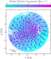 |
Fig. 12. Two-dimensional distribution of stars in local Cartesian coordinates (x; y). Stars are color-coded according to the inferred mean radial component of the velocity in their Voronoi bin, while black arrows show the mean velocity vector in each bin. Radial velocity is defined as positive if pointing away from the center, thus |


The same pattern emerges when computing the mean radial velocity  in spherical shells (see Eq. (4)), as shown in Fig. 13. In particular, the innermost 2° show a flat slightly positive profile (
 ) indicating central expansion, although the radial motion is highly dominated by random motion (
 ). However, moving toward larger radii, the contraction (
 ) becomes increasingly more prominent and the radial motion more ordered.
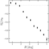 |
Fig. 13. Radial profile of the ratio of the radial mean velocity to the radial velocity dispersion computed in spherical shells. Black dots show the median values, while quoted errors are the 16th and 84th percentiles of the distributions. The dashed horizontal line shows the zero expansion–contraction level. |
The robustness of the contraction pattern (Figs. 12 and 13) was tested against the assumption of a particular bulk LOS velocity when accounting for perspective expansion (since we had only a few measurements). We considered the worst-case scenario in which stars followed the LOS velocity distribution expected for the MW field stars in the region ( km s−1 and σLOS, MW ≃ 20 km s−1, see Fig. 10).
The transverse motions were then corrected by randomly assigning to each star a LOS velocity extracted from the MW-like distribution. We iterated this procedure 100 times finding that the velocity pattern observed was weakly affected by our mean bulk motion assumption and the contraction showed in Fig. 13 was always recovered.
4.3. Mass dependence analysis
The presence of a mass spectrum has a non-negligible role in the dynamics of both young and old stellar systems. Old stellar clusters are indeed known to naturally develop mass segregation due to two-body interactions that cause significant kinetic energy exchange among stars and cause massive stars to sink toward the cluster’s center (Binney & Tremaine 2008). However, evidence of mass segregation has also been found in younger Galactic clusters (e.g., Hillenbrand & Hartmann 1998; Gouliermis et al. 2004; Stolte et al. 2006; Evans & Oh 2022), thus possibly implying a connection with the early stages of cluster formation (McMillan et al. 2007; Allison et al. 2009; Livernois et al. 2021). In addition, numerical simulations showed that during the violent relaxation phase, young stellar systems can start developing a dependence of the kinematical properties (rotation, velocity dispersion) on the stellar mass (see, e.g., Livernois et al. 2021). The investigation of possible mass-dependent dynamical properties is therefore crucial to shed further light on the dynamics of young stellar systems.
We estimated stellar masses using theoretical M–G0 relation for zero age main sequence stars. This relation was obtained from the PARSEC models for a population of 14 Myr in age (the youngest age we estimate) with [Fe/H]= − 0.3 dex. Stellar masses were therefore derived by interpolation of this relation, and in Fig. 14 we show the spatial distribution of stars color-coded by their mass.
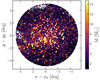 |
Fig. 14. Spatial distribution of stars color-coded by mass. Masses were obtained by mass-absolute magnitude relation (see text for further details). |
Figure 14 indicates that massive stars (lighter symbols) are more centrally concentrated than lower mass ones (darker symbols). We thus quantitatively investigated this feature by looking at the cumulative profiles in different mass bins, after correcting for completeness (see Fig. 4) by assigning to each star a weight = 1/completeness. We limited the analysis to stars more massive than 1.1 M⊙ to avoid very low completeness values. Figure 15 shows that the massive stars exhibited a more centrally concentrated spatial distribution than the lower mass ones. In addition, a Kolmogorov-Smirnov test confirmed the statistical significance of this result (p < 0.003) for every combination of mass bins. In Appendix A we show the completeness distributions for each mass bin.
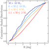 |
Fig. 15. Cumulative radial profiles constructed in four different mass bins from stars with masses between 1.1–2 M⊙ (in red) up to stars more massive than 10 M⊙ (in dark blue). Stellar counts were corrected for incompleteness star by star. |
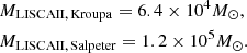
Finally, we looked for evidence of a dependence of the kinematic properties on the stellar masses. In Fig. 16 we show the velocity dispersion profiles constructed for different mass bins, specifically for stars with mass M ≤ 2 M⊙ (red symbols), 2 M⊙ < M ≤ 4 M⊙ (light blue symbols) and M > 4 M⊙ (dark blue symbols).
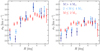 |
Fig. 16. Velocity dispersion profiles in the radial (left panel) and tangential (right panel) components, in three different mass bins depicted with different colors: red for the least massive bin and dark blue for the most massive. |
Our analysis reveals mild evidence of a dependence of the velocity dispersion on the stellar mass within about 2° from the center in both the radial and tangential components: more massive stars show a slightly smaller velocity dispersion. At radii R > 2 − 3 deg the velocity dispersion profiles become indistinguishable and no signs of equipartition are found. The trend is consistent with that expected for a stellar system that has started to evolve toward energy equipartition during its early evolutionary phases and is in general agreement with the trends found in the simulations presented in Livernois et al. (2021). We discuss this point further in Sect. 7.
Finally, we observed an increase in the velocity dispersion moving away from the center in every mass bin (variations up to ∼0.6 km s−1, see Fig. 16). Several effects might be at play in driving such a pattern, for instance deviation from spherical symmetry (see, e.g., the color-coded map in Fig. 12, whose expansion pattern was clearly nonspherical), a nonconstant mean velocity within bins (as noted by Da Rio et al. 2017), and possibly the presence of residual field interlopers.
We also observed a clear dependence of the radial velocity component on the stellar mass. In particular, stars more massive than about ≳2 M⊙ exhibit a higher positive mean radial velocity (up to about 1 km s−1) than lower mass stars within the innermost 3° (see Fig. 17), while at larger radii massive stars contract toward the center ( ) with a similar slope to lower mass stars, albeit with a higher normalization.
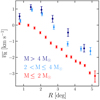 |
Fig. 17. Mean radial velocity profiles for stars in three different mass bins: M ≤ 2 M⊙ (red symbols), 2 < M ≤ 4 M⊙ (light blue symbols), and M > 4 M⊙ (dark blue symbols). Positive values of |

We thus further investigated this feature in the 2D plane using the Voronoi tessellation, giving particular attention to non-spherically symmetric features and putative links with the spatial distribution of stars. In Fig. 18 we show 2D maps of mean radial velocity for stars with mass above (left panel) and below (right panel) 2 M⊙. Expansion ( ) is depicted in purple, contraction (
 ) is depicted in blue, and black lines highlight iso-probability contours of the density distribution of the respective populations.
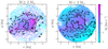 |
Fig. 18. Two-dimensional maps of mean radial velocity for high-mass stars (M ≥ 2 M⊙, left panel) and low-mass stars (right panel). Stars belonging to the same Voronoi bin are color-coded according to the mean radial velocity, while black lines are iso-density contours of the respective populations enclosing about 12% (solid line), 39% (dashed line), and 67% (dash-dotted line) of the underlying density distribution. |
Interestingly, a clear connection between expansion and density comes up when looking at massive stars (left panel of Fig. 18), suggesting that higher-density regions expand faster than lower ones, whereas no clear connection is found for the low-mass population (right panel). In addition, we found consistent features to what is observed in Fig. 17: massive stars expand faster than lower mass ones, which in turn had higher contraction speeds in the outskirts.
The spectro-photometric (i.e., age and metallicity), structural (i.e., density profiles and mass segregation), and kinematic (i.e., contraction and equipartition) evidence collected so far suggests that the stars selected within a few degrees of NGC 654 are not just a group of co-moving stars; rather, the nine identified clusters and the extended low-density halo surrounding them are part of a common, substructured, and still-forming massive stellar system. Following the definition introduced in Dalessandro et al. (2021b), we named it LISCA II.
5. Structure and kinematic of the embedded star clusters
In this section we present the structural and kinematic properties of the nine star clusters composing LISCA II.
First, we constructed the number density radial profiles for all the clusters (following the same approach described in Sect. 4) with respect to their center of mass, and we fitted them with the Plummer (Plummer 1911) and King (King 1962) models. Figure 19 shows the observed profiles and the models, normalized to the clusters’ central densities and observed projected half-mass radii (Rhm) enabling a quantitative comparison among different clusters. The quantity Rhm is defined as the projected radius that encloses half of the total cluster’s mass directly obtained from the radial distribution of member stars.
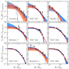 |
Fig. 19. Number density profiles (black symbols) for the nine star clusters. Also shown are the model predictions for the Plummer (red) and King (blue) models. Shaded areas represent the 68% credible regions. All the profiles, both observed and models, were scaled to the central density predicted by the Plummer model Σ0, plummer and to the observed projected half-mass radius Rhm. |
Every star cluster exhibits a cluster-like profile that, within the errors, is equally well modeled by both the Plummer and King models, with the only exception of NGC 581 (see Fig. 19), which exhibits a sharper truncation not captured by the Plummer model.
In addition, we present the kinematic properties of star clusters: Fig. 20 shows the inferred 1D velocity dispersion, which is defined as
 (5)
(5)
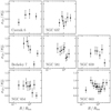 |
Fig. 20. One-dimensional velocity dispersion profiles for seven out of nine star clusters. Velocity dispersion was normalized to the same quantity computed for all the cluster’s members ( |

with σR and σT being the projected radial and tangential components of the velocity dispersion inferred assuming the likelihood in Eq. (4) and sampling the parameter space with an MCMC technique.
For two clusters, namely Riddle 4 and Berkeley 6, we could not compute reliable kinematic profiles since few stars (51 and 84 respectively) fulfilled the astrometric quality selections presented in Sect. 4.
All the other clusters exhibit rather flat dispersion profiles that can be hardly explained by equilibrium models, for instance those adopted to fit the stellar density distributions. Several effects might be at play in producing the observed flat dispersion profiles, such as contaminants from the stellar halo and dynamical heating due to tidal interactions with other clusters and substructures possibly taking place during the system’s early evolution. We discuss dynamical heating in more detail in Sect. 7.
To estimate the total mass of each cluster we followed the same approach described in Dalessandro et al. (2021b), and we normalized a Kroupa (2001) and a Salpeter (1955) initial mass function (IMF) in the range M > 4 M⊙, such that the number of member stars matched the number predicted by direct integration of the IMF
 (6)
(6)
with mmin = 4 M⊙ and mmax = 11 − 14 M⊙ for every cluster but Berkeley 6, whose maximum stellar mass is approximately 7 M⊙ according to its inferred age. Once the normalization was obtained, we computed the total visible mass by integrating the IMF in the range Mmin − Mmax = 0.09 − 14.73 M⊙
 (7)
(7)
respectively the minimum and maximum stellar mass for a 14 Myr-old simple stellar population with [Fe/H]= − 0.3 dex (Bressan et al. 2012). The derived cluster masses are in the range ≃0.5 − 5.6 × 10³ M⊙ (≃0.7 − 8.8 × 10³ M⊙) according to a Kroupa (Salpeter) IMF.
The main kinematic and structural properties of the clusters are summarized in Table 1. Specifically, for each cluster we included the coordinates of the center of mass (for stars more massive than 2 M⊙), the mean parallax and proper motion (of the distributions shown in Fig. 1) along with errors, the Plummer scale length and the King core radius (obtained from the models shown in Fig. 19 and converted to parsec using the mean parallax also reported in Table 1), the total masses inferred by assuming either a Kroupa or a Salpeter IMF, and finally the total number of member stars for each cluster.
Star cluster properties obtained in this study.
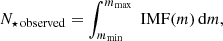
6. Total system mass
The total mass of LISCA II was estimated by using Eq. (7) and roughly the same approach as for the single clusters. However, in this case, we had to assume a radial extension of the system within which to integrate the stellar masses. To this end we used the Jacobi radius (RJ; see, e.g., Binney & Tremaine 2008) as a first-order physically plausible radial extension of the system. The radius RJ is simply defined as
 (8)
(8)
with R0 ≃ 10.2 kpc and  M⊙ being the galactocentric distance of the system and the MW mass enclosed within that radius, respectively (Cautun et al. 2020), and MLISCAII is the total system mass. Starting from Eq. (8), we estimated both RJ and the mass of the system by using an iterative procedure until final convergence was reached. Depending on the assumed IMF we obtain
 (9)
(9)
with the corresponding enclosed (< 2RJ) masses being
 (10)
(10)
It is important to note here that in this case RJ is only meant to provide a general indication of the spatial scale related to the strength of the tidal field at the location of LISCA II. In the complex case of a clumpy system far from a spherical configuration in dynamical equilibrium like that of LISCA II, the detailed implications of the effects of the tidal field truncation for this system would require a tailored set of simulations. We also note that the kinematical properties revealed by our analysis (Sect. 4) indicate that in this system all the stars, including those beyond the present estimate of RJ, are strongly contracting toward the center of the system, which is just the opposite of what is expected for stars escaping the system.
7. Comparison with N-body simulations of early cluster evolution
In this section we present an analysis of the dynamical properties of one of the N-body models studied in Livernois et al. (2021). The simulations of Livernois et al. (2021) explored the early evolution and violent relaxation phases of young rotating star clusters and followed their evolution from a hierarchical structure to a final monolithic equilibrium configuration.
We note that our goal here is not to build a detailed model of the LISCA II system, but rather to gather further insight into our observational analysis. Hence, here we just provide a theoretical example of the general dynamical properties expected in a hierarchical stellar cluster undergoing its early evolutionary phases. The model we analyzed for this paper is the F025 model of Livernois et al. (2021). The model is fully described in Livernois et al. (2021), but we summarize its main features for the purposes of this study. The model starts with 105 stars with mass range 0.08 − 100 M⊙, initially following a fractal distribution with a fractal dimension equal to 2.6; the system is initially dynamically cold and undergoes the collapse and subsequent structural oscillations typical of the violent relaxation phase. As a reference timescale for the presentation of our results, we adopt the system free-fall timescale, tff, which corresponds approximately to the timescale needed for the system to reach its maximum contraction during its initial collapse. Assuming an initial mass of 5 × 10⁴ − 105 M⊙ and an initial radius of ∼50 − 60 pc, the tff would roughly correspond to 20 − 35 Myr. To capture the model at multiple evolutionary stages, we focus our attention on the snapshots at the following values of t/tff: 0.9 (denoted TFF09), 1.1 (TFF11), 1.3 (TFF13), 1.5 (TFF15), and 1.7 (TFF17).
7.1. Mass segregation and bulk internal motion
We start our analysis with the study of mass segregation in the N-body model and the LISCA II system. Here we focus on an analysis specifically aimed at detecting mass segregation on a local scale, which might provide further insight into the dynamics of systems characterized by the presence of clumps and substructures like those studied here. To quantify the level of mass segregation, we first calculate the local surface number density for each star using the distance of the sixth nearest star of any mass (Casertano & Hut 1985); the median local surface density of different mass bins, normalized by the median local surface density of the entire cluster, is plotted against the median stellar mass of each bin in Fig. 21. All snapshots show clear evidence of a local surface density increasing with the stellar mass, implying the presence of local-scale mass segregation, where massive stars are migrating toward the centers of the subclusters they are members of. A similar trend is also present in LISCA II, which shows significant local-scale mass segregation, complementing the global-scale mass segregation found in Fig. 15. This trend appears to evolve with time in the model snapshots; the two latest snapshots have the strongest trend of local-scale mass segregation.
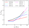 |
Fig. 21. Local number density of stars as a function of stellar mass (see Sect. 7.1). The local density is normalized by the median local surface density of the entire cluster. The increase in local density with stellar mass indicates mass segregation on local scales across all clusters shown. |
Focusing on the bulk internal motion of the system, we analyzed the radial velocity profile of the simulation data as a comparison to Fig. 13. In Fig. 22, we plot the radial velocity profile normalized by the velocity dispersion of the cluster, including only stars with m > 2 M⊙. As the cluster evolves, we see the different regions of the cluster transition between expansion and contraction. The TFF09 snapshot is characterized by a trend similar to that found in LISCA II: an expansion of the inner regions and a strong contraction in the outer regions.
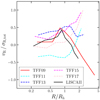 |
Fig. 22. Projected radial velocity profiles for each snapshot of the N-body simulation and the LISCA II system. The projected radius is normalized to the projected half-mass radius of the system in each snapshot, and the radial velocity is normalized to the radial velocity dispersion of all stars in the system. |
7.2. Dynamics of subclusters
For insight into the possible dynamical evolution of the subclusters within LISCA II, we analyzed the dynamical properties of selected clumps from our N-body models. For each snapshot in the N-body data, we selected a few clumps in spherical 3D regions and determined their centers as the location of the maximum local density. These clumps are in dynamically active environments, and no clustering metrics were found to be appropriate across all snapshots for clump identification.
We start by showing in Fig. 23 the surface density profile (top panel) and LOS velocity dispersion profile (bottom panel) for the clumps selected in the TFF09 snapshot. We fit a Plummer model based on the surface density profile and enclosed mass within one projected half-mass radius, and overplot the best-fit model lines. All clumps show radial variation of the surface density profiles following the general shape of the Plummer model; on the other hand, the velocity dispersion profiles are flatter and more elevated than is expected from the best-fit Plummer models. This is the manifestation of the tidal heating in the cluster environment and is similar to what is seen in Fig. 20.
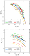 |
Fig. 23. Surface density profiles (top) and 1D velocity dispersion profiles (bottom) for the TFF09 snapshot. The best-fit Plummer model for each clump is also shown (dashed lines). The best-fit Plummer model is determined by fitting the surface density profile within one projected half-mass radius. The surface density and 1D velocity dispersion are both normalized to the corresponding values in the innermost radial bin of each clump. |
We repeated the above analysis for all of our snapshots, and plot in Fig. 24 the average ratio of the surface density (top panel) and LOS velocity dispersion (bottom panel) to the best-fit Plummer models across the three biggest clumps in each snapshot. The surface density fits well out to approximately one projected half-mass radius, outside of which the clumps generally have a higher density than the best-fit Plummer model; these deviations from the best-fit Plummer model can be attributed to the high density of the surrounding environment and the perturbations due to interactions in the cluster environment. The effects of these perturbations are clearly visible in the LOS velocity dispersion profiles of all the snapshots analyzed. All the velocity dispersion profiles deviate from the profiles expected from the best-fit Plummer models across all radii with a dependence on the projected radius that varies in different snapshots.
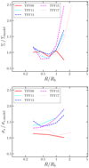 |
Fig. 24. Radial profiles of the ratio of the clump radial profiles to the best-fit Plummer models for surface density (top) and 1D velocity dispersion (bottom). This ratio is averaged over the three largest clumps within each snapshot. |
Finally, we summarized the relation between structural and kinematic perturbations by plotting, in Fig. 25, the ratio of density and LOS velocity dispersion to the corresponding values of these quantities from the best-fit Plummer models at Rh for the three biggest clumps in each snapshot. This plot clearly shows that the fingerprints of the highly active environment, where each clump is undergoing rapid interactions, mergers, and fragmentations, are more evident in the kinematic properties, as illustrated by the larger deviations of the velocity dispersion from the expected equilibrium values.
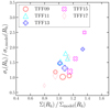 |
Fig. 25. One-dimensional velocity dispersion vs. projected surface density for the three largest clumps in each snapshot (see legend), each calculated at one projected half-mass radius. The 1D velocity dispersion and the projected surface density are both normalized by the value expected from the Plummer model best fitting the surface density profile. Point sizes are proportional to the total mass of each clump. |
8. Discussion and conclusions
The unprecedented quality of the Gaia DR3 data (Gaia Collaboration 2023, supplemented by high-resolution spectra (Fanelli et al. 2022) obtained as part of the SPA-TNG large program, allowed us to identify the LISCA II system in the Perseus complex.
The spectro-photometric, structural, and kinematical properties of this system are in generally good agreement with those theoretically expected from the early dynamical evolution of a massive molecular cloud that experienced violent relaxation and is now in the process of hierarchically assembling its stellar constituents and evolving toward a monolithic structure. In particular, the observed evidence of mass segregation on a local and global scale, the mass-dependent kinematic properties, and out-of-equilibrium internal kinematics of individual subclusters, as well as the observation of a dominant contraction pattern toward the system center mainly driven by the external regions of LISCA II and of a milder central expansion, are compatible with what is expected in the early evolutionary phases of stellar systems assembling as a coherent massive structure by N-body models. The properties of these hierarchical stellar systems are shaped by a combination of large-scale variations of the system’s potential and smaller scale interactions of individual subclusters and clumps.
Although more detailed models and additional data would be necessary to further explore the possible fate of this system, the evidence collected in this paper suggests that LISCA II is a good candidate to evolve into a young massive (104 − 105 M⊙) star cluster on a timescale of ∼100 Myr, corresponding to a few free-fall times. These results make LISCA II the second structure, the first being LISCA I (Dalessandro et al. 2021b), ever found in the MW in the process of hierarchically assembling in a massive stellar cluster. LISCA II is located at only ∼6 deg from LISCA I, with which it shares similar chemical composition ([Fe/H] = − 0.30 dex), age (t ∼ 20 Myr), and overall mass.
In conclusion, the present analysis has provided a comprehensive characterization of the process of cluster assembly with a level of detail that cannot be achieved in external galaxies or at high redshift (where the progenitors of the oldest clusters formed), thus showing that probing cluster formation in local environments can help shed light on the physical processes involved in massive cluster formation and their role in determining the cluster’s dynamical properties. Moreover, we further showed that hierarchical cluster assembly is a viable process, even in low-density environments such as the MW (former observational evidence was mainly in high-density environments, e.g., Bastian et al. 2011; Chandar et al. 2011), and a statistical assessment of its effectiveness on Galactic scales is the subject of an ongoing study. It is interesting to note in this respect that the possible observed internal age spreads of the stellar populations belonging to LISCA I and II (∼10 Myr) nicely fit the observed trend (Parmentier et al. 2014) between the cluster formation environment stellar density and final cluster age internal variations, which possibly results from the different duration of the star formation processes and the link between their efficiency and the systems’ free-fall time. This further strengthens the idea that clusters with different present-day properties likely underwent similar formation processes.
We refer to the online documentation (https://hdbscan.readthedocs.io/en/latest/index.html) for further details.
We use the subscript “0” for reddening-corrected magnitudes and not for absolute ones, i.e., they are not corrected for dimming due to the distance.
Throughout the paper we use the expression radial velocity to denote the radial component of the velocity projected onto the plane of the sky, whereas LOS velocity denotes the component aligned with the observer’s LOS.
Acknowledgments
The authors thank the anonymous referee for the careful reading of the paper and the useful comments and suggestions. A.D.C., E.D. and L.O. acknowledge financial support from the project Light-on-Dark granted by MIUR through PRIN2017-2017K7REXT contract. E.D. acknowledges support from the Indiana University Institute for Advanced Study through the Visiting Fellowship program. This work uses data from the European Space Agency (ESA) space mission Gaia. Gaia data are being processed by the Gaia Data Processing and Analysis Consortium (DPAC). Funding for the DPAC is provided by national institutions, in particular, the institutions participating in the Gaia Multi-Lateral Agreement (MLA).
References
- Adamo, A., Kruijssen, J. M. D., Bastian, N., Silva-Villa, E., & Ryon, J. 2015, MNRAS, 452, 246 [NASA ADS] [CrossRef] [Google Scholar]
- Allison, R. J., Goodwin, S. P., Parker, R. J., et al. 2009, ApJ, 700, L99 [Google Scholar]
- Allison, R. J., Goodwin, S. P., Parker, R. J., Portegies Zwart, S. F., & de Grijs, R. 2010, MNRAS, 407, 1098 [NASA ADS] [CrossRef] [Google Scholar]
- Ballone, A., Mapelli, M., Di Carlo, U. N., et al. 2020, MNRAS, 496, 49 [NASA ADS] [CrossRef] [Google Scholar]
- Ballone, A., Torniamenti, S., Mapelli, M., et al. 2021, MNRAS, 501, 2920 [NASA ADS] [CrossRef] [Google Scholar]
- Banerjee, S. 2021, MNRAS, 500, 3002 [Google Scholar]
- Banerjee, S., & Kroupa, P. 2014, ApJ, 787, 158 [NASA ADS] [CrossRef] [Google Scholar]
- Banerjee, S., & Kroupa, P. 2015, MNRAS, 447, 728 [NASA ADS] [CrossRef] [Google Scholar]
- Bastian, N., & Lardo, C. 2018, ARA&A, 56, 83 [Google Scholar]
- Bastian, N., Adamo, A., Gieles, M., et al. 2011, MNRAS, 417, L6 [NASA ADS] [Google Scholar]
- Beccari, G., Boffin, H. M. J., Jerabkova, T., et al. 2018, MNRAS, 481, L11 [Google Scholar]
- Binney, J., & Tremaine, S. 2008, Galactic Dynamics: Second Edition [Google Scholar]
- Bonaca, A., Conroy, C., Cargile, P. A., et al. 2020, ApJ, 897, L18 [NASA ADS] [CrossRef] [Google Scholar]
- Bonnell, I. A., Bate, M. R., & Vine, S. G. 2003, MNRAS, 343, 413 [NASA ADS] [CrossRef] [Google Scholar]
- Bovy, J., Hogg, D. W., & Roweis, S. T. 2011, Ann. Appl. Stat., 5, 1657 [Google Scholar]
- Bressan, A., Marigo, P., Girardi, L., et al. 2012, MNRAS, 427, 127 [NASA ADS] [CrossRef] [Google Scholar]
- Brodie, J. P., & Strader, J. 2006, ARA&A, 44, 193 [Google Scholar]
- Brüns, R. C., & Kroupa, P. 2011, ApJ, 729, 69 [CrossRef] [Google Scholar]
- Cantat-Gaudin, T. 2022, Universe, 8, 111 [NASA ADS] [CrossRef] [Google Scholar]
- Cantat-Gaudin, T., & Anders, F. 2020, A&A, 633, A99 [NASA ADS] [CrossRef] [EDP Sciences] [Google Scholar]
- Cantat-Gaudin, T., Anders, F., Castro-Ginard, A., et al. 2020, A&A, 640, A1 [NASA ADS] [CrossRef] [EDP Sciences] [Google Scholar]
- Cantat-Gaudin, T., Fouesneau, M., Rix, H.-W., et al. 2023, A&A, 669, A55 [NASA ADS] [CrossRef] [EDP Sciences] [Google Scholar]
- Cappellari, M., & Copin, Y. 2003, MNRAS, 342, 345 [Google Scholar]
- Cardelli, J. A., Clayton, G. C., & Mathis, J. S. 1989, ApJ, 345, 245 [Google Scholar]
- Casertano, S., & Hut, P. 1985, ApJ, 298, 80 [Google Scholar]
- Castro-Ginard, A., Jordi, C., Luri, X., et al. 2022, A&A, 661, A118 [NASA ADS] [CrossRef] [EDP Sciences] [Google Scholar]
- Cautun, M., Benítez-Llambay, A., Deason, A. J., et al. 2020, MNRAS, 494, 4291 [Google Scholar]
- Chambers, K. C., Magnier, E. A., Metcalfe, N., et al. 2016, ArXiv e-prints [arXiv:1612.05560] [Google Scholar]
- Chandar, R., Whitmore, B. C., Calzetti, D., et al. 2011, ApJ, 727, 88 [Google Scholar]
- Cosentino, R., Lovis, C., Pepe, F., et al. 2014, in Ground-based and Airborne Instrumentation for Astronomy V, eds. S. K. Ramsay, I. S. McLean, & H. Takami, SPIE Conf. Ser., 9147, 91478C [Google Scholar]
- Da Rio, N., Tan, J. C., Covey, K. R., et al. 2017, ApJ, 845, 105 [Google Scholar]
- Dalessandro, E., Schiavon, R. P., Rood, R. T., et al. 2012, AJ, 144, 126 [NASA ADS] [CrossRef] [Google Scholar]
- Dalessandro, E., Cadelano, M., Vesperini, E., et al. 2018, ApJ, 859, 15 [NASA ADS] [CrossRef] [Google Scholar]
- Dalessandro, E., Raso, S., Kamann, S., et al. 2021a, MNRAS, 506, 813 [CrossRef] [Google Scholar]
- Dalessandro, E., Varri, A. L., Tiongco, M., et al. 2021b, ApJ, 909, 90 [NASA ADS] [CrossRef] [Google Scholar]
- de Oliveira, M. R., Dottori, H., & Bica, E. 1998, MNRAS, 295, 921 [NASA ADS] [CrossRef] [Google Scholar]
- Di Carlo, U. N., Giacobbo, N., Mapelli, M., et al. 2019, MNRAS, 487, 2947 [NASA ADS] [CrossRef] [Google Scholar]
- Evans, N. W., & Oh, S. 2022, MNRAS, 512, 3846 [NASA ADS] [CrossRef] [Google Scholar]
- Everall, A., & Boubert, D. 2022, MNRAS, 509, 6205 [Google Scholar]
- Everall, A., Boubert, D., Koposov, S. E., Smith, L., & Holl, B. 2021, MNRAS, 502, 1908 [CrossRef] [Google Scholar]
- Fanelli, C., Origlia, L., Oliva, E., et al. 2022, A&A, 660, A7 [NASA ADS] [CrossRef] [EDP Sciences] [Google Scholar]
- Ferraro, F. R., Mucciarelli, A., Lanzoni, B., et al. 2018, ApJ, 860, 50 [NASA ADS] [CrossRef] [Google Scholar]
- Forbes, D. A., Read, J. I., Gieles, M., & Collins, M. L. M. 2018, MNRAS, 481, 5592 [NASA ADS] [CrossRef] [Google Scholar]
- Foreman-Mackey, D., Hogg, D. W., Lang, D., & Goodman, J. 2013, PASP, 125, 306 [Google Scholar]
- Fujii, M. S., & Portegies Zwart, S. 2016, ApJ, 817, 4 [NASA ADS] [CrossRef] [Google Scholar]
- Gaia Collaboration (Brown, A. G. A., et al.) 2021, A&A, 649, A1 [NASA ADS] [CrossRef] [EDP Sciences] [Google Scholar]
- Gaia Collaboration (Vallenari, A., et al.) 2023, A&A, in press, https://doi.org/10.1051/0004-6361/202243940 [Google Scholar]
- Gavagnin, E., Mapelli, M., & Lake, G. 2016, MNRAS, 461, 1276 [NASA ADS] [CrossRef] [Google Scholar]
- Getman, K. V., Feigelson, E. D., Kuhn, M. A., & Garmire, G. P. 2019, MNRAS, 487, 2977 [Google Scholar]
- Gieles, M., Portegies Zwart, S. F., Baumgardt, H., et al. 2006, MNRAS, 371, 793 [Google Scholar]
- Gouliermis, D., Keller, S. C., Kontizas, M., Kontizas, E., & Bellas-Velidis, I. 2004, A&A, 416, 137 [NASA ADS] [CrossRef] [EDP Sciences] [Google Scholar]
- Gratton, R., Bragaglia, A., Carretta, E., et al. 2019, A&A Rev., 27, 8 [NASA ADS] [CrossRef] [Google Scholar]
- Grillmair, C. J. 2019, ApJ, 884, 174 [Google Scholar]
- Hénault-Brunet, V., Gieles, M., Evans, C. J., et al. 2012, A&A, 545, L1 [NASA ADS] [CrossRef] [EDP Sciences] [Google Scholar]
- Hillenbrand, L. A., & Hartmann, L. W. 1998, ApJ, 492, 540 [NASA ADS] [CrossRef] [Google Scholar]
- Hong, J., de Grijs, R., Askar, A., et al. 2017, MNRAS, 472, 67 [NASA ADS] [CrossRef] [Google Scholar]
- Hunt, E. L., & Reffert, S. 2021, A&A, 646, A104 [NASA ADS] [CrossRef] [EDP Sciences] [Google Scholar]
- Jerabkova, T., Boffin, H. M. J., Beccari, G., et al. 2021, A&A, 647, A137 [NASA ADS] [CrossRef] [EDP Sciences] [Google Scholar]
- Kamann, S., Husser, T. O., Dreizler, S., et al. 2018, MNRAS, 473, 5591 [NASA ADS] [CrossRef] [Google Scholar]
- Katz, D., Sartoretti, P., Cropper, M., et al. 2019, A&A, 622, A205 [NASA ADS] [CrossRef] [EDP Sciences] [Google Scholar]
- King, I. 1962, AJ, 67, 471 [Google Scholar]
- Kounkel, M., & Covey, K. 2019, AJ, 158, 122 [Google Scholar]
- Kroupa, P. 2001, MNRAS, 322, 231 [NASA ADS] [CrossRef] [Google Scholar]
- Kruijssen, J. M. D. 2012, MNRAS, 426, 3008 [Google Scholar]
- Krumholz, M. R., McKee, C. F., & Bland-Hawthorn, J. 2019, ARA&A, 57, 227 [NASA ADS] [CrossRef] [Google Scholar]
- Kuhn, M. A., Hillenbrand, L. A., Sills, A., Feigelson, E. D., & Getman, K. V. 2019, ApJ, 870, 32 [CrossRef] [Google Scholar]
- Kuhn, M. A., Hillenbrand, L. A., Carpenter, J. M., & Avelar Menendez, A. R. 2020, ApJ, 899, 128 [NASA ADS] [CrossRef] [Google Scholar]
- Lada, C. J., & Lada, E. A. 2003, ARA&A, 41, 57 [Google Scholar]
- Lada, C. J., Margulis, M., & Dearborn, D. 1984, ApJ, 285, 141 [NASA ADS] [CrossRef] [Google Scholar]
- Lee, Y. W., Joo, J. M., Sohn, Y. J., et al. 1999, Nature, 402, 55 [Google Scholar]
- Li, C., Sun, W., de Grijs, R., et al. 2019, ApJ, 876, 65 [Google Scholar]
- Lim, B., Hong, J., Yun, H.-S., et al. 2020, ApJ, 899, 121 [CrossRef] [Google Scholar]
- Lindegren, L., Bastian, U., Biermann, M., et al. 2021, A&A, 649, A4 [EDP Sciences] [Google Scholar]
- Livernois, A., Vesperini, E., Tiongco, M., Varri, A. L., & Dalessandro, E. 2021, MNRAS, 506, 5781 [NASA ADS] [CrossRef] [Google Scholar]
- Madau, P., & Dickinson, M. 2014, ARA&A, 52, 415 [Google Scholar]
- Mann, H., & Whitney, D. 1947, Ann. Math. Stat., 18, 50 [Google Scholar]
- McInnes, L., Healy, J., & Astels, S. 2017, J. Open Source Software, 2, 205 [NASA ADS] [CrossRef] [Google Scholar]
- McKee, C. F., & Ostriker, E. C. 2007, ARA&A, 45, 565 [Google Scholar]
- McMillan, S. L. W., Vesperini, E., & Portegies Zwart, S. F. 2007, ApJ, 655, L45 [Google Scholar]
- Meingast, S., Alves, J., & Fürnkranz, V. 2019, A&A, 622, L13 [NASA ADS] [CrossRef] [EDP Sciences] [Google Scholar]
- Meingast, S., Alves, J., & Rottensteiner, A. 2021, A&A, 645, A84 [NASA ADS] [CrossRef] [EDP Sciences] [Google Scholar]
- Miller, G. E., & Scalo, J. M. 1979, ApJS, 41, 513 [Google Scholar]
- Moeckel, N., & Bonnell, I. A. 2009, MNRAS, 400, 657 [NASA ADS] [CrossRef] [Google Scholar]
- Moeckel, N., & Bate, M. R. 2010, MNRAS, 404, 721 [NASA ADS] [CrossRef] [Google Scholar]
- Oliva, E., Origlia, L., Maiolino, R., et al. 2012, in Ground-based and Airborne Instrumentation for Astronomy IV, eds. I. S. McLean, S. K. Ramsay, & H. Takami, SPIE Conf. Ser., 8446, 84463T [NASA ADS] [Google Scholar]
- Pang, X., Li, Y., Yu, Z., et al. 2021, ApJ, 912, 162 [NASA ADS] [CrossRef] [Google Scholar]
- Pang, X., Tang, S.-Y., Li, Y., et al. 2022, ApJ, 931, 156 [NASA ADS] [CrossRef] [Google Scholar]
- Parker, R. J. 2014, MNRAS, 445, 4037 [NASA ADS] [CrossRef] [Google Scholar]
- Parmentier, G., Pfalzner, S., & Grebel, E. K. 2014, ApJ, 791, 132 [NASA ADS] [CrossRef] [Google Scholar]
- Plummer, H. C. 1911, MNRAS, 71, 460 [Google Scholar]
- Pryor, C., & Meylan, G. 1993, in Structure and Dynamics of Globular Clusters, eds. S. G. Djorgovski, & G. Meylan, ASP Conf. Ser., 50, 357 [Google Scholar]
- Raso, S., Libralato, M., Bellini, A., et al. 2020, ApJ, 895, 15 [NASA ADS] [CrossRef] [Google Scholar]
- Robin, A. C., Reylé, C., Derrière, S., & Picaud, S. 2003, A&A, 409, 523 [NASA ADS] [CrossRef] [EDP Sciences] [Google Scholar]
- Salpeter, E. E. 1955, ApJ, 121, 161 [Google Scholar]
- Saydjari, A. K., Schlafly, E. F., Lang, D., et al. 2023, ApJS, 264, 28 [NASA ADS] [CrossRef] [Google Scholar]
- Schlafly, E. F., & Finkbeiner, D. P. 2011, ApJ, 737, 103 [Google Scholar]
- Schlafly, E. F., Green, G. M., Lang, D., et al. 2018, ApJS, 234, 39 [Google Scholar]
- Schlegel, D. J., Finkbeiner, D. P., & Davis, M. 1998, ApJ, 500, 525 [Google Scholar]
- Spina, L., Ting, Y. S., De Silva, G. M., et al. 2021, MNRAS, 503, 3279 [CrossRef] [Google Scholar]
- Stolte, A., Brandner, W., Brandl, B., & Zinnecker, H. 2006, AJ, 132, 253 [NASA ADS] [CrossRef] [Google Scholar]
- Tarricq, Y., Soubiran, C., Casamiquela, L., et al. 2021, A&A, 647, A19 [NASA ADS] [CrossRef] [EDP Sciences] [Google Scholar]
- Tiongco, M. A., Vesperini, E., & Varri, A. L. 2022, MNRAS, 512, 1584 [NASA ADS] [CrossRef] [Google Scholar]
- Tozzi, A., Oliva, E., Iuzzolino, M., et al. 2016, in Ground-based and Airborne Instrumentation for Astronomy VI, eds. C. J. Evans, L. Simard, & H. Takami, SPIE Conf. Ser., 9908, 99086C [NASA ADS] [Google Scholar]
- Treviño-Morales, S. P., Fuente, A., Sánchez-Monge, Á., et al. 2019, A&A, 629, A81 [NASA ADS] [CrossRef] [EDP Sciences] [Google Scholar]
- van Leeuwen, F. 2009, A&A, 497, 209 [CrossRef] [EDP Sciences] [Google Scholar]
- Vasiliev, E., & Baumgardt, H. 2021, MNRAS, 505, 5978 [NASA ADS] [CrossRef] [Google Scholar]
- Zeidler, P., Sabbi, E., Nota, A., & McLeod, A. F. 2021, AJ, 161, 140 [NASA ADS] [CrossRef] [Google Scholar]
Appendix A: Completeness distributions in different mass bins
In this Appendix we show the completeness distributions for the five-parameter solutions in the four different mass bins used to investigate the presence of mass segregation (see Figure 15). As can be seen, the higher the mass, the higher the completeness. The distribution width is due to both a finite mass range in the bin and differential reddening, which link the estimated mass to the observed G magnitude.
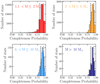 |
Fig. A.1. Completeness distribution in four mass bins. Colors are consistent with Figure 15 and the mass range is shown in the upper left corner. |
All Tables
All Figures
|
Fig. 1. Inferred distributions in parallax (top panel) and proper motion (bottom panel) from likely (> 90%) cluster members. Different stellar clusters are in different colors. Dashed gray lines in the bottom panel are iso-probability contours at the 1, 2, and 3σ levels. The red dashed circle and vertical lines represent the range in proper motion and parallax inside which stars were selected. |
| In the text | |
|
Fig. 2. Spatial distribution in Galactic coordinates of stars selected in proper motion and parallax. Star cluster names are shown in blue, while black lines are iso-density contours enclosing 11.8% (solid), 39.3% (dashed), and 67.5% (dash-dotted) of the normalized star density distribution. The black arrow shows the direction of the Galactic center (GC). |
| In the text | |
|
Fig. 3. Two-dimensional map of the p(G) term in Eq. (1) for G = 19.5 mag, computed with the GaiaUnlimited package (Cantat-Gaudin et al. 2023). White points show the location of star clusters. |
| In the text | |
|
Fig. 4. Catalog completeness in the five-parameter solution estimated from star count ratios (p(5params|G) term in Eq. (2)) for G = 18.5 mag (left panel) and G = 19.5 mag (right panel). White points give the positions of star clusters. |
| In the text | |
|
Fig. 5. Color-magnitude diagram for NGC 663 members. In black the observed photometry, while in red and blue are shown the distributions of stars after correcting for differential reddening. For the former Galactic extinction maps by Schlegel et al. (1998), Schlafly & Finkbeiner (2011) are used, and for the latter the reddening corrections estimated in this work. |
| In the text | |
|
Fig. 6. Two-dimensional reddening map in Galactic coordinates. The extinction was computed star by star from color-color diagrams (see text for further details). White areas correspond to regions devoid of stars. |
| In the text | |
|
Fig. 7. Observed (left panel) and differential reddening corrected (right panel) CMD for the full catalog. In blue we show stars with LOS velocity measurements from Gaia DR3 (big squares for stars considered in the LOS analysis), whereas in red are stars targeted by high-resolution spectroscopy. The subsample with chemical abundances is circled in red. |
| In the text | |
|
Fig. 8. Cumulative luminosity function for the stellar cluster NGC 654 (gray histogram), along with the normalized histogram of a 32 Myr old synthetic population computed with the PARSEC model (blue histogram). The error bars show the standard deviation of the model’s count fluctuations due to several extractions (see text for further details). Bins are 0.5 mag wide. |
| In the text | |
|
Fig. 9. Color-magnitude diagrams of cluster members (black dots) corrected for differential reddening. For each cluster, the best-fit isochrone is shown in blue and the median age along with the 68% credible interval is also reported. The shaded areas show the region inside which stars are flagged as supergiants. |
| In the text | |
|
Fig. 10. LOS velocity (left panel) and iron-over-hydrogen abundance (right panel) distributions for members of the selected structure (gray histogram) and for a Milky Way model (blue histogram). The intrinsic dispersions are also shown in the top left corners. All the distributions are scaled by a constant factor for visualization purposes only. |
| In the text | |
|
Fig. 11. Stellar number density profile of an 8° region around the system’s center of mass and considering stars brighter than G = 18 mag. The observed profile is shown in gray, while the intrinsic profile (after background subtraction) is shown in black. The Plummer model (in red) and the King model (in blue) are also shown, along with the corresponding 68% credible regions constructed from the posterior samples. |
| In the text | |
|
Fig. 12. Two-dimensional distribution of stars in local Cartesian coordinates (x; y). Stars are color-coded according to the inferred mean radial component of the velocity in their Voronoi bin, while black arrows show the mean velocity vector in each bin. Radial velocity is defined as positive if pointing away from the center, thus |
| In the text | |
|
Fig. 13. Radial profile of the ratio of the radial mean velocity to the radial velocity dispersion computed in spherical shells. Black dots show the median values, while quoted errors are the 16th and 84th percentiles of the distributions. The dashed horizontal line shows the zero expansion–contraction level. |
| In the text | |
|
Fig. 14. Spatial distribution of stars color-coded by mass. Masses were obtained by mass-absolute magnitude relation (see text for further details). |
| In the text | |
|
Fig. 15. Cumulative radial profiles constructed in four different mass bins from stars with masses between 1.1–2 M⊙ (in red) up to stars more massive than 10 M⊙ (in dark blue). Stellar counts were corrected for incompleteness star by star. |
| In the text | |
|
Fig. 16. Velocity dispersion profiles in the radial (left panel) and tangential (right panel) components, in three different mass bins depicted with different colors: red for the least massive bin and dark blue for the most massive. |
| In the text | |
|
Fig. 17. Mean radial velocity profiles for stars in three different mass bins: M ≤ 2 M⊙ (red symbols), 2 < M ≤ 4 M⊙ (light blue symbols), and M > 4 M⊙ (dark blue symbols). Positive values of |
| In the text | |
|
Fig. 18. Two-dimensional maps of mean radial velocity for high-mass stars (M ≥ 2 M⊙, left panel) and low-mass stars (right panel). Stars belonging to the same Voronoi bin are color-coded according to the mean radial velocity, while black lines are iso-density contours of the respective populations enclosing about 12% (solid line), 39% (dashed line), and 67% (dash-dotted line) of the underlying density distribution. |
| In the text | |
|
Fig. 19. Number density profiles (black symbols) for the nine star clusters. Also shown are the model predictions for the Plummer (red) and King (blue) models. Shaded areas represent the 68% credible regions. All the profiles, both observed and models, were scaled to the central density predicted by the Plummer model Σ0, plummer and to the observed projected half-mass radius Rhm. |
| In the text | |
|
Fig. 20. One-dimensional velocity dispersion profiles for seven out of nine star clusters. Velocity dispersion was normalized to the same quantity computed for all the cluster’s members ( |
| In the text | |
|
Fig. 21. Local number density of stars as a function of stellar mass (see Sect. 7.1). The local density is normalized by the median local surface density of the entire cluster. The increase in local density with stellar mass indicates mass segregation on local scales across all clusters shown. |
| In the text | |
|
Fig. 22. Projected radial velocity profiles for each snapshot of the N-body simulation and the LISCA II system. The projected radius is normalized to the projected half-mass radius of the system in each snapshot, and the radial velocity is normalized to the radial velocity dispersion of all stars in the system. |
| In the text | |
|
Fig. 23. Surface density profiles (top) and 1D velocity dispersion profiles (bottom) for the TFF09 snapshot. The best-fit Plummer model for each clump is also shown (dashed lines). The best-fit Plummer model is determined by fitting the surface density profile within one projected half-mass radius. The surface density and 1D velocity dispersion are both normalized to the corresponding values in the innermost radial bin of each clump. |
| In the text | |
|
Fig. 24. Radial profiles of the ratio of the clump radial profiles to the best-fit Plummer models for surface density (top) and 1D velocity dispersion (bottom). This ratio is averaged over the three largest clumps within each snapshot. |
| In the text | |
|
Fig. 25. One-dimensional velocity dispersion vs. projected surface density for the three largest clumps in each snapshot (see legend), each calculated at one projected half-mass radius. The 1D velocity dispersion and the projected surface density are both normalized by the value expected from the Plummer model best fitting the surface density profile. Point sizes are proportional to the total mass of each clump. |
| In the text | |
|
Fig. A.1. Completeness distribution in four mass bins. Colors are consistent with Figure 15 and the mass range is shown in the upper left corner. |
| In the text | |
Current usage metrics show cumulative count of Article Views (full-text article views including HTML views, PDF and ePub downloads, according to the available data) and Abstracts Views on Vision4Press platform.
Data correspond to usage on the plateform after 2015. The current usage metrics is available 48-96 hours after online publication and is updated daily on week days.
Initial download of the metrics may take a while.