| Issue |
A&A
Volume 674, June 2023
|
|
|---|---|---|
| Article Number | A85 | |
| Number of page(s) | 15 | |
| Section | Catalogs and data | |
| DOI | https://doi.org/10.1051/0004-6361/202245437 | |
| Published online | 07 June 2023 | |
Classifying the full SDSS-IV MaNGA Survey using optical diagnostic diagrams: Presentation of AGN catalogs in flexible apertures★
Zentrum für Astronomie der Universität Heidelberg, Astronomisches Rechen-Institut,
Mönchhofstr, 12–14
69120
Heidelberg, Germany
e-mail: malban@uni-heidelberg.de
Received:
11
November
2022
Accepted:
15
February
2023
Accurate active galactic nucleus (AGN) identifications in large galaxy samples are crucial for the assessment of the role of AGN and AGN feedback in the co-evolution of galaxies and their central supermassive black holes. Emission-line flux-ratio diagnostics are commonly used to identify AGN in optical spectra. New large samples of integral field unit observations allow exploration of the role of aperture size in the classification process. In this paper, we present galaxy classifications for all 10010 galaxies observed within the Mapping Nearby Galaxies at Apache Point Observatory (MaNGA) survey. We use Baldwin-Philips-Terlevich line flux-ratio diagnostics combined with an Hα equivalent threshold in 60 apertures of varying size for the classification, and provide the corresponding catalogs. MaNGA-selected AGN primarily lie below the main sequence of star-forming galaxies, and reside in massive galaxies with stellar masses of ~1011 M⊙ and a median Hα-derived star formation rate of ~1.44M⊙ yr−1. We find that the number of “fake” AGN increases significantly beyond selection apertures of >1.0 Reff because of increased contamination from diffuse ionized gas (DIG). A comparison with previous works shows that the treatment of the underlying stellar continuum and flux measurements can significantly impact galaxy classification. Our work provides the community with AGN catalogs and galaxy classifications for the full MaNGA survey.
Key words: catalogs / galaxies: active
AGN catalogs and FITS are only available at the CDS via anonymous ftp to cdsarc.cds.unistra.fr (130.79.128.5) or via https://cdsarc.cds.unistra.fr/viz-bin/cat/J/A+A/674/A85
© The Authors 2023
 Open Access article, published by EDP Sciences, under the terms of the Creative Commons Attribution License (https://creativecommons.org/licenses/by/4.0), which permits unrestricted use, distribution, and reproduction in any medium, provided the original work is properly cited.
This article is published in open access under the Subscribe to Open model. Subscribe to A&A to support open access publication.
1 Introduction
Mounting observational evidence shows that supermassive black holes (SMBHs) are ubiquitous in the centers of most, and perhaps all, massive galaxies (Decarli et al. 2007; Kormendy & Ho 2013; Graham 2016). Many properties of these galaxies show tight relations (e.g., the velocity dispersion of the bulge, Ferrarese & Merritt 2000; Gültekin et al. 2009), in particular with the mass of their SMBH (Beifiori et al. 2011), suggesting that the presence of a SMBH impacts the evolution of the host galaxy and vice versa. How this happens over cosmic time is an active field of study (e.g., Heckman & Best 2014; Park et al. 2015; Volonteri et al. 2016; Buchner et al. 2019; Smith & Bromm 2019; Singh et al. 2021). Standard evolution models invoke the active growth phases of SMBHs, that is, their active galactic nucleus (AGN; Rees 1984; Alexander & Hickox 2012; Padovani et al. 2017) phase.
While an SMBH is active, the injection of energy into the interstellar medium (ISM) generated by accretion onto the BH can have a relevant impact on the host galaxy, leading, for example, to the quenching (negative feedback; Springel et al. 2005; Cano-Díaz et al. 2012) or enhancement of star formation (positive feedback; Mahoro et al. 2017; Nesvadba et al. 2020; Bessiere & Almeida 2022), or even both (e.g., Wagner et al. 2016; Dugan et al. 2017). This has motivated authors to build cosmological simulations (see Somerville & Davé 2015, for a detailed review) that include AGN feedback (Fabian 2012) in their models.
To constrain and accurately quantify the effect that AGN have on their host galaxies, AGN-selection algorithms must be as complete as possible. AGN galaxies show a very wide range of peculiar observational characteristics (Maoz 2007), and it is therefore not surprising that all AGN-selection methods come with some caveats. Over recent decades, multiple AGN-selection methods have been invoked that are inspired by the peculiar multiwavelength radiation from the energetic release of the accretion onto SMBHs (for a convenient summary of these methods, see Sect. 1.4 of Harrison 2014). However, these techniques can be heavily biased towards, for example, finding AGN preferentially in luminous host galaxies or may not be sufficiently sensitive to find obscured AGN (e.g., Azadi et al. 2017; Yi et al. 2022).
A commonly used AGN-selection method is based on strong optical emission-line ratios (Baldwin et al. 1981; Veilleux & Osterbrock 1987), which are frequently visualized as BPT diagrams in the literature; we adopt this nomenclature here. The used line complexes are close in wavelength space, which reduces the effects of dust reddening that could affect the measurement of the emission-line ratios (Kennicutt 1992). This technique, together with empirical demarcation lines (for the demarcation line equations and a summary of this methods; see Kewley et al. 2006), allows us to distinguish between different ionization sources. For example, star-forming galaxies and HII regions exhibit specific line ratios that tend to occupy a well-defined area in the BPT diagram. Other celestial objects, such as planetary nebula, and most importantly (for our study, to identify AGN activity) Seyfert and low-ionization nuclear emission-line region galaxies (LINERs; Halpern & Steiner 1983) gather in different positions on the BPT diagram. A frequently used BPT diagnostic diagram includes [O III]λ5008/Hβ versus [N II]λ6583/Hα, which can be used to distinguish between AGN-like galaxies and star-forming galaxies, with an overlapping region that classifies objects as composite galaxies (which show characteristics consistent with both AGN and star-forming galaxies; Kewley et al. 2001). However, this diagram alone does not allow LINERs to be distinguished from and Seyfert galaxies.
LINER galaxies were originally proposed to be driven by weak accretion-powered AGN (Halpern & Steiner 1983; Kauffmann et al. 2003a; Ho 2008; Masegosa et al. 2011), presenting lower ionization levels (Ferland & Netzer 1983) compared to Seyferts. Therefore, additional BPT diagrams use [O III]/Hβ versus [SII] λλ6717,6731/Hα (Kewley et al. 2001) and [OIII]/Hβ versus [OI] λ6302/Hα (Kauffmann et al. 2003a) to further distinguish between LINER and Seyfert galaxies. However, some LINERs have also been reported to be compatible with galaxies whose spectral contribution is dominated by ionizing photons from post-asymptotic giant branch stars (e.g., Binette et al. 1994; Yan & Blanton 2012; Singh et al. 2013) or to be related to post-starburst galaxies (Taniguchi et al. 2000). This situation motivated authors to use alternative diagnostics to select true AGN from the LINER galaxy population. For example, Cid Fernandes et al. (2010) proposed the use of an additional cut in Hα equivalent width (EW) motivated by the fact that Seyfert galaxies have higher EW(Hα) values than LINER galaxies without AGN.
Some difficulties in using BPT diagnostics (see Sect. 5 of Kewley et al. 2019, for a review) also arise that are due to the fact that emission line ratios can be affected by shocks (e.g., Dopita et al. 2002; Allen et al. 2008), obscuration by dust, metallicity (as the BPT diagram correlates with metallicity; Groves et al. 2004), diffuse ionized gas regions (Zhang et al. 2016; Mannucci et al. 2021), morphology, and cosmic time (Kewley et al. 2013; Hirschmann et al. 2017). Furthermore, observational effects, such as using different aperture sizes, affect measurements of integrated galaxy properties, such as integrated star formation rates, emission line fluxes, or EW(Hα) measurements (Hopkins et al. 2003; Gómez et al. 2003; Kewley et al. 2005; Iglesias-Páramo et al. 2016). Naturally, galaxy classification using BPT diagnostics is therefore highly dependent on aperture size (Maragkoudakis et al. 2014). If the galaxies to be classified span a range in redshift, a constant aperture probes different physical sizes in the observed galaxies. This directly affects the observed emission-line flux ratios in single-fiber spectral observations, possibly leading to misclassifications (Veilleux et al. 1995; Maragkoudakis et al. 2014).
Integral field spectroscopy (IFS; Bershady et al. 2010; Drory et al. 2015) can help mitigate this effect by allowing us to map the 2D spectral properties of a target (e.g., Westfall et al. 2019). In particular, the SDSS-IV survey Mapping Nearby Galaxies at APO (MaNGA) provides optical IFU observations of 10010 galaxies at 0.03 < z < 0.1. The final data release DR17 was recently been released to the public (DR17; Abdurro'uf et al. 2022). In the present paper, we investigate the impact of aperture effects for BPT-based AGN classifications and provide a suite of AGN catalogs based on three sets of apertures with differing units (kpc, effective radius, and arcseconds). We classify galaxies as “star-forming”, Seyfert, “composite”, LINER, or “ambiguous”.
The paper is organized as follows: In Sect. 2, we describe the data and some available AGN catalogs from early and recent MaNGA product launches and data releases. The details of the method we use to study the sample and the AGN-selection algorithm are described in Sect. 3. In Sect. 4 we present our aperture-based catalog and discuss the impact of the aperture selection. We compare our AGN candidates with other AGN catalogs in Sect. 5. Finally, we present our conclusions in Sect. 6. Throughout the paper we use H0 =72 km s−1 Mpc−1, ΩM=0.3, and ΩΛ = 0.7.
2 Data and AGN catalogs
2.1 MaNGA DR17
MaNGA (Bundy et al. 2015) is one of the surveys of the fourth generation of the Sloan Digital Sky Survey (SDSS-IV). It is an IFU survey providing spatially resolved spectra (Drory et al. 2015; Law et al. 2015) covering a spectral range from 3622 to 10354 Å at a resolution of R~2000 for each target using the 2.5 Sloan Telescope (Gunn et al. 2006). The field of view of the IFU ranges from 12 to 32 arcsec in diameter, ensuring that at least 80% of the targets are covered out to 1.5 Re and 2.5 Re, respectively. The 17th (and last) data release (Abdurro'uf et al. 2022) includes data for 10010 unique galaxies at 0.01 < z < 0.15 with stellar masses > 109 M⊙.
For MaNGA, a Data Reduction Pipeline (DRP) is provided in Law et al. (2016), the output of which is processed by the Data Analysis Pipeline (DAP; Westfall et al. 2019; Belfiore et al. 2019). In the DRP, the raw data for each target are calibrated, sky-subtracted, and stored in individual datacubes and row-stacked spectra. The DAP then analyzes the latter to create cubes with the binned spectra together with models for the best-fit spectra for different components (e.g., stellar continuum, emission lines). The DAP also provides maps of physical properties of the galaxies (e.g., sky coordinates and kinematics, such as stellar and gas velocities, emission line fluxes, equivalent widths, etc.). Throughout this paper, we use the emission-line measurements (see Sect. 3) from the DAP for our analysis.
A set of AGN catalogs (e.g., Rembold et al. 2017; Wylezalek et al. 2018; Sánchez et al. 2018; Comerford et al. 2020) from previous SDSS-IV releases has provided AGN candidates since the early stages of MaNGA (e.g., MaNGA Product Launch 5, hereby MPL-5). These catalogs are described in the coming subsections and are used for comparison purposes (see Sect. 5) to examine possible differences with our selection technique in Sect. 3.2. We provide a detailed comparison of the ionized gas dynamics in AGN selected using different methods in an upcoming paper (Albán et al., in prep.).
2.2 MaNGA-MPL-5 AGN catalog of Sánchez et al. (2018)
By June 2016, MaNGA had observed around 2700 targets (MaNGA Product Launch 5 or MPL-5; the MPL5 sample is identical to the 14th data release of MaNGA; Abolfathi et al. 2018). For this sample, Sánchez et al. (2018) found 98 AGN candidates. In this latter study, the authors used optical diagnostics (BPT diagrams), following the guidelines from Kewley et al. (2006) on the three BPT classification diagrams ([N II]/Hα, [S II]/Hα, and [O I]/Hα). They focus on the emission-line fluxes inside a 3″ aperture derived using the PIPE3D (Sánchez et al. 2016) data-analysis pipeline. In addition to the BPT diagnostics, the authors also include a cut in EW(Hα) of > 1.5Å (Cid Fernandes et al. 2010). A classification between type-I and type-II AGN (see Antonucci 1993; Netzer 2015, for a detailed overview on AGN types) is also provided based on a multi-Gaussian emission-line-fitting procedure in the spectral region containing Hα and [N II]. The authors classify an AGN as type-I if the broad component satisfies the following criteria: S/N > 5 and 1000 < FWHM < 10000 km s−1. Sánchez et al. (2018) identify 35 type-I AGN in their sample.
2.3 MaNGA-MPL-5 AGN catalog of Rembold et al. (2017)
An additional study by Rembold et al. (2017) identified 62 AGN candidates in the MaNGA MPL-5/DR14 galaxy sample. These authors follow a similar approach to that described in Sect. 2.2, using optical-BPT diagnostics. However, the analysis is carried out using only one, namely the [N II]-based BPT diagnostic. The authors use emission-line fluxes from a 3″×3″ aperture, but do not use the MaNGA data directly for their analysis. Instead, they use measurements from the SDSS-III single-fiber observations. The emission line fluxes and EW(Hα) were taken from the spectral analysis of Thomas et al. (2013), which requires an amplitude-over-noise (AoN) of greater than two to calculate an emission-line flux. Rembold et al. (2017) apply an EW(Hα) > 3 Å cut, as in Cid Fernandes et al. (2010). The latter criterion is also used in our AGN selection.
2.4 MaNGA-MPL-5 AGN catalog of Wylezalek et al. (2018)
A different approach was used in Wylezalek et al. (2018). Ionization radiation due to AGN can sometimes be found far away from the center of galaxies. Possible reasons for this effect are central obscuration, recent mergers, and relic AGN (e.g., Keel et al. 2015). Therefore, Wylezalek et al. (2018) developed a selection procedure based on spatially resolved BPT maps taking full advantage of IFU spectra and do not require AGN-like BPT diagnostics in the galaxy centers.
In addition to the classical BPT line ratio diagnostics, they impose a suite of additional criteria to circumvent potential contamination of their sample through diffuse ionized gas, extra-planar gas, and photoionization by hot stars. These authors detect 303 AGN candidates in the same MaNGA Product Launch (MPL-5), and find 173 galaxies that would not have been selected as AGN candidates using the standard selection algorithms based on single-fiber spectral observations.
2.5 MaNGA-MPL8 multiwavelength AGN catalog of Comerford et al. (2020)
Comerford et al. (2020) used mid-infrared (MIR), X-ray, and radio observations as well as broad emission lines in SDSS spectra to identify 406 AGN in the MaNGA MPL-8 (6261 galaxies) catalog. Their AGN catalog is thus independent of any BPT diagnostics. They find 67 AGN through MIR selection criteria using data from the Wide-field Infrared Survey Explorer (WISE; Wright et al. 2010), 17 using hard-X-ray selection criteria from Burst Alert Telescope (BAT; Barthelmy et al. 2005) observations, and 325 AGN candidates through radio selection criteria using data from the NRAO Very Large Array Sky Survey (NVSS; Condon et al. 1998) and the Faint Images of the Radio Sky at Twenty centimeters (FIRST; Becker et al. 1995) survey. In their catalog, Comerford et al. (2020) also subdivide radio-selected AGN into radio-loud and radio-quiet AGN. Additionally, they present 55 type-1 AGN candidates based on broad Balmer emission lines in SDSS spectra. Some galaxies are classified as AGN by several of these criteria (e.g., 11 galaxies were classified as AGN simultaneously by radio and MIR selection criteria; see Table 2 in Comerford et al. 2020).
3 AGN selection
In this section, we present how IFU spectroscopy can be used in a variety of ways to classify MaNGA galaxies according to their BPT diagnostics. We extract the emission-line properties of the targets in different aperture sizes and investigate how optical diagnostics vary and depend on the chosen aperture size. We finally present a suite of BPT-based MaNGA AGN catalogs with varying apertures for the full MaNGA sample (DR17).
3.1 Sample definition
To obtain the emission-line fluxes, as required by a BPT classification, we extract the emission-line maps for [O III]λ5008, [N II]λ6584, [S II]λλ6717,6731 (hereafter, we refer to the sum of [S II]λλ6717,6731 simply as [S II]), [O I]λ6300, and the hydrogen Balmer lines Hα and Hβ from the DAP. We use their nonparametric emission-line measurements. The latter are derived using bands of 20 Å centered on each emission line, and a narrower passband is used for Hα and [N II] because of their small separation (see Westfall et al. 2019). No special treatment is used for possible complexities in emission lines such as galactic outflows (e.g., Wylezalek et al. 2020) or emission from the broad line region (BLR; Peterson 2006; Netzer 2015). We use the MANGA_DAPPIXMASK1 bitmap to mask pixels flagged as DONOTUSE or UNRELIABLE in order to exclude biased and/or unreliable measurements.
Furthermore, in each map, we mask the pixels where the emission line flux does not satisfy a signal-to-noise ratio (S/N) of greater than three (the S/N is also extracted from the DAP). Emission lines with a S/N < 3 lead to unreliable flux measurements and therefore unreliable emission-line ratios, which would increase the bias in the classification (e.g., Brinchmann et al. 2004). We measure the pixel-weighted flux before computing the emission-line ratios. When a pixel (at a certain position) in a map of a specific parameter (e.g., the [N II] flux) has a S/N < 3, we do not use that pixel for computing the emission line flux of that aperture (see Sect. 3.2). However, if that pixel (same position as before) has a sufficiently high S/N (S/N > 3) in another map (e.g., the [S II] flux) of the same galaxy, it is included for computing that emission line flux.
This S/N cut inevitably decreases the size of our galaxy sample. For example, when using an aperture of 2 kpc (see Sect. 3.3), in ~25% of the MaNGA galaxies no pixels are left available for measuring emission line fluxes due to the S/N cut. Therefore, our sample is biased towards line-emitting galaxies, which are preferentially gas-rich, star-forming galaxies. We explore this bias further in Sects. 4.3 and 4.4.
3.2 Optical classification
Because of the IFU nature of the MaNGA observations, we can perform an aperture-dependent optical classification. We perform weighted averages such that if a pixel partially contributes to a circular (or squared) aperture, we weigh the pixel according to the fraction of its enclosed area. The latter is measured as follows:

where xi is the total contribution of the pixel and wi is the weight of the pixel measured as the fraction of the enclosed area by the corresponding aperture for the N enclosed pixels. We construct a squared grid to represent the area and position of each pixel. Each pixel is placed in the center of the squares of the grid, which are evenly distributed according to the average distance between the original coordinates (as in the coordinate map, known as SPX_SKYCOO, from the DAP maps).
We compare the coordinate of the center of each square (from the grid) to the original center (from the DAP map SPX_SKYCOO) of the pixel. The typical offsets between the coordinates of our synthetic grid and those from the DAP are of the order of 10−8″, and the distances from each pixel are of the order of 10−2″, demonstrating that the deviations from the original position of the pixels are negligible. Therefore, we do not take into account this effect when calculating average emission-line fluxes inside the respective apertures. An example of this interpolation is shown in Fig. 1, where in the left plot we display an example of the [O III]λ5008 emission-line flux map (masked as described in Sect. 3.1) with the aperture shown with a black circle (whose size corresponds to 2 kpc). The right plot shows a zoomed-in version of this map using a different color map based on the fraction of the pixel enclosed by the aperture (again shown in black); we note that pixels whose area enclosed by the aperture is zero are masked as NaN values and are excluded from the plot. To create a specific aperture, the digital size of a pixel is converted to physical quantities using data from the DAP (e.g., effective radius, pixel per arcsecond, and kiloparsec steps) and the DRP (for individual redshifts using the NSA redshift measurements).
We measure average emission-line fluxes in a set of apertures following the quality criteria outlined in Sect. 3.1. We then compute the following average flux ratios: [O III]/Hβ [N II]/Hα, [S II]/Hα, and [O I]/Hα (also with a S/N > 3 cut). For a specific aperture (e.g., 2 kpc or 3″×3″), we perform two separate classifications (Kewley et al. 2001, 2006; Kauffmann et al. 2003a): one using all three BPT diagrams and one excluding the [O I]6300/Hα BPT diagram. The [O I]6300 emission line is weaker than the other lines in the BPT diagrams and therefore exhibits a lower S/N. This would therefore lead to the exclusion of many more galaxies from the analysis (see Tables 1 and 2). If a galaxy is classified as one type in one diagram and as a different type in the remaining diagrams (whether we are using two or three of the diagrams), this galaxy will be labeled as ambiguous. Additionally, we also apply the diagnostic criteria outlined by Cid Fernandes et al. (2010), which allows the differentiation between two very distinct classes of galaxies that overlap in the LINER region of the BPT diagrams, namely galaxies hosting a weak AGN and “retired galaxies”. Retired galaxies have stopped forming stars and are ionized by their hot evolved low-mass stars, namely post-AGB stars. This differentiation can be achieved using an equivalent width (EW) cut of EW(Hα) > 3 Å. We use the EW(Hα) from the DAP and also measure its average (see Eq. (1)) in the various apertures. We apply this EW(Hα) cut to all galaxies above star-forming demarcation lines (Kewley et al. 2006). This step concludes the classification procedure. As mentioned in Sect. 3.1, we were not able to classify all galaxies because of the quality cuts. We refer to these low-S/N galaxies as the unclassified ones (see Sect. 4.4).
We point out that we have not taken into account the inclination angles of the individual galaxies, meaning that all the circular or squared apertures are performed on the line-of-sight projected galaxy.
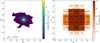 |
Fig. 1 Example of our weighted pixel averaging. The left plot shows (target with plate-ifu: 8725-9102) the flux of the [OIII]λ5007 emission line. Pixels with S/N < 3 are masked. The black circle indicates the 2 kpc circular diameter aperture where we average the flux for the emission line ratios. The right plot shows a zoom onto the aperture region, showing the percentage of the pixel area captured by the aperture shown in black. We show the value in each pixel that corresponds to the weight of the pixel when we compute the average fluxes. |
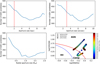 |
Fig. 2 Variation in AGN classification with different aperture sizes. The y-axis in the top plots and the bottom left plot shows the number of galaxies classified as AGN (solid blue line) selected based on different aperture sizes and using different units. The selection is made following the algorithm described in Sect. 3.2, excluding the [O I]/Hα BPT diagram. In the top left plot, the kiloparsec aperture increases in steps of 0.5 kpc (in diameter). In the top right plot, the arcsecond aperture increases in steps of 0.5″ (in diameter). In the bottom left plot, the effective radius aperture increases in steps of 0.1 Reff (in radius). The red (vertical-dashed) line in the top panels corresponds to the apertures used for the comparisons in Sect. 5. In the bottom right plot, we show how the flux ratios in one BPT diagram change as a function of the aperture. This is done for three individual galaxies illustrated with different symbols (see the legend for their corresponding MaNGA-IDs). Each symbol is filled with a specific color that corresponds to the size of its aperture. In the bottom right plot, we also include the empirical division lines that will give each target a specific classification (e.g., AGN-like galaxy, composite object, or HII-star forming galaxies): red lines correspond to Kewley et al. (2001), and the blue dashed line on the left plot corresponds to Kauffmann et al. (2003a). |
MaNGA-DR17 catalog for optical diagnostics classification excluding the [O I] BPT diagram using a 2 kpc and a 3″×3″ aperture.
MaNGA-DR17 catalog for optical diagnostics classification including the [O I] BPT diagram using a 2 kpc and a 3″×3″ aperture.
3.3 Aperture effects on BPT AGN selection
In this section, we explore the behavior of an aperture-dependent classification. To do so, we investigate the BPT classification as described in Sect. 3.2 in 60 different apertures of different sizes, defined as follows:
Twenty circular apertures with sizes ranging from 0.5 kpc to 10 kpc in diameter in steps of 0.5 kpc.
Twenty square apertures with sizes ranging from 0.5″ to 10″ on the side in steps of 0.5″.
Twenty circular apertures with sizes ranging from 0.1 Reff to 2 Reff in diameter in steps of 0.1 Reff.
In Fig. 2 (bottom right plot), we show an example of the behavior of the emission-line ratios from three different targets when using 20 circular apertures. This reveals the dependence of the classification on the chosen aperture. In Fig. 2 (see the two upper plots and the one to the bottom left), we show how the number of galaxies classified as AGN changes as a function of an increasing kpc-, arcsecond-, and effective radius (Reff)-based aperture, respectively. For simplicity, we use the term “AGN” to refer to “galaxies classified as AGN” hereafter.
As expected, in the smallest apertures, and independently of the specific unit, the number of galaxies classified as AGN is similar. However, the number of AGN in Reff-based apertures drops steeply (compared to the other apertures) and reaches its minimum at ~0.7–1 Reff. This happens because the step that we use based on effective radius aperture reaches the outskirts of the galaxies faster, leading to fewer galaxies classified as AGN. In the ~7500 galaxies that we were able to classify (see Table 1), the average Reff corresponds to ~4.63 kpc, meaning that an aperture of 0.7 Reff will have an average size of ~6.5 kpc in diameter.
We also observe an initial decrease in the total number of classified AGN in the kpc- and arcsec-based apertures. We then observe an increase in classified AGN at larger aperture sizes in all panels. The increasing number of AGN at larger aperture sizes is most notably seen in the kpc- and arcsec-based apertures (see the top panels of Fig. 2) beyond ~6 kpc and ~7″, respectively (see Sect. 4.1). In the Reff-based apertures, the number of AGN increases beyond ~1.2 Reff.
For all the targets in MaNGA DR17, we provide FITS tables containing all of our relevant measurements (emission-line ratios and Hα EWs, if available) in all apertures investigated here. We report the BPT class of each galaxy (before applying the EW cut and excluding the [O I]6300/Hα diagram) and the resulting AGN catalog for each specific aperture. We provide these catalogs as part of the supplementary material. We show an example of one of our catalogs in Table 3, specifically for the 2 kpc-based classification. We note that (as discussed in Sect. 3.2) for a galaxy to be classified as an AGN, our procedure not only requires the emission-line ratios to be located above the star-forming demarcation lines (see Kewley et al. 2006) but also to have an EW(Hα) of greater than 3 (whether they are selected as Seyfert or LINER). For example, in row number 8528, the target is classified as Seyfert initially, but because of a low EW(Hα) this target fails to meet our final AGN criteria. The same is true for the LINER galaxy in row number 8529. Due to our S/N criteria, some values are stored as NaN, and thus we do not assign any classification (e.g., 8531; we note that these targets do not even enter the ambiguous BPT classification). In row number 8535, a Seyfert met the EW(Hα) cut and is selected as an AGN candidate. In that case, the [O I]/Hα column is NaN, but this does not impact the classification, as [O I]/Hα is not used here. The classifications and measurements in these catalogs can be used according to the science goals. The most obvious advantage is the ability to choose parameters and classifications from a specific aperture. For example, one can alternatively decide to relax on the EW(Hα) criterion when selecting AGN (if needed), and select AGN from the Seyfert and LINER population with EW(Hα)> 1.5 Å. Therefore, it is possible to easily extract modified classifications from these catalogs.
BPT classification (without using [O I]/Hα), AGN selection, emission-line ratios, and equivalent-width values for the MaNGA galaxies.
3.4 Aperture effects on BPT type classification
In Fig. 3, we show how the classification in individual BPT sub-types (i.e., star-forming, Seyfert, LINER, composites, ambiguous) changes as a function of aperture size. For this analysis, we choose the BPT classification, using only the [N II] and [S II] BPT diagrams derived from a kpc-based aperture (the color coding corresponds to the Hα surface brightness, which we discuss in detail in Sect. 4.1). Specifically, at an aperture size of ~ 2 kpc, the number of star-forming galaxies reaches its maximum value, while the number of ambiguous objects and the number of Seyfert galaxies decreases beyond this aperture. At very large aperture sizes, we see a drastic decrease in the galaxies classified as star-forming as the number of galaxies classified as LINER and ambiguous galaxies increases. This effect is explored in Sects. 4.1 and 4.3.
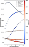 |
Fig. 3 Number of galaxies (y-axis) identified by a specific BPT classification (see the legend to the top right of the plot) using different selection aperture sizes (in kpc, x-axis). Each value is colored according to the average Hα surface brightness (color bar) within a 2 kpc aperture. This classification is done excluding the [O I] BPT diagram. |
4 Analysis
4.1 The role of diffuse ionized gas
Early studies of radio observations and optical emission lines provided evidence for the existence of diffuse ionized components outside bright H II regions and in kpc-scale layers extending above 1–2 kpc of the Galactic Plane as well as in nearby galaxies (Hoyle & Ellis 1963; Reynolds 1984; Rand et al. 1990). The diffuse ionized gas (DIG; see Haffner et al. 2009, for a review) is an important element of the ISM (and currently an active field of study; e.g., Belfiore et al. 2016; Zhang et al. 2016; Jones et al. 2017; Wylezalek et al. 2018; Vale Asari et al. 2019; Krishnarao et al. 2020; Mannucci et al. 2021), corresponding to a widespread (low density ~ 0.1 cm−3), warm gas (10000 K). Zhang et al. (2016) showed that DIG typically has low Hα surface brightness and can significantly affect emission-line ratios and thus the typical optical diagnostics, suggesting that choosing galaxies or spaxels with ΣHα>1039 erg s−1 kpc−2 will result in more reliable H II-dominated regions. DIG can not only drive true star-forming galaxies to the ambiguous and LINER-like BPT classification regime but can also imitate AGN-like emission-line ratios.
Although IFU surveys provide an excellent observational tool for studying the spatially resolved properties of galaxies, individual MaNGA spaxels resolve properties down to kpc scales. Therefore, it is inevitable that multiple ionizing sources contribute to individual spaxels, which include contamination from DIG-dominated regions. In Fig. 2, we see that apertures exceeding 6 kpc, 7″, and 1.2 Reff start to detect “AGN candidates” at larger radii. As discussed in Sect. 4.2, we expect reliable AGN signatures from the inner kpc regions of true AGN candidates. Therefore, we explore the potential role of the DIG in affecting the increasing AGN-detection rate at larger apertures.
To do so, we measure the cumulative2 radial profiles of the Hα surface brightness for all MaNGA targets following the procedure in Sect. 3.2. We stack the cumulative radial profiles of the AGN-selected galaxies from a 2 kpc (diameter) aperture (419 galaxies) and a 10 kpc aperture (381 galaxies). Additionally, we compute the stacked radial profile using the AGN candidates that were selected by the 10 kpc aperture, excluding the AGN that were selected in both the 2 kpc and 10 kpc apertures (158 galaxies). The latter was done only using the [N II] and [S II] BPT diagrams. The results are shown in Fig. 4. All the AGN-selected galaxies from a 2 kpc (diameter) aperture (green solid line) show a high central Hα surface brightness (ΣHα ~ 1039.5 erg s−1 kpc−2) and a higher cumulative radial profile when compared to the AGN selected only based on the 10 kpc aperture (i.e., excluding the ones selected from the 2 kpc aperture). These 10 kpc AGN candidates display a lower central surface brightness (ΣHα<1039 erg s−1 kpc−2). Both populations (2 kpc and 10 kpc selected) show significantly different levels and distributions of Hα surface brightness at every radius, with a difference of almost 1 dex.
We find this systematic decrease in the Hα surface brightness to be consistent with an increasing contribution from DIG regions. This explains the increase in galaxies classified as AGN in larger apertures observed in Fig. 2, which suggests that an increasing aperture would lead to the inclusion of a DIG-biased population of AGN candidates. We further study this in Fig. 3, where we show the number of AGN candidates with a specific classification (each represented with a different shape) when using different selection apertures. The color map in this figure shows the average Hα surface brightness measured in a 2 kpc aperture for each data point. Here, the number of targets classified as LINER (circles) and ambiguous (triangles) galaxies increases at larger apertures while the average Hα surface brightness (measured at a 2 kpc aperture) decreases and is generally at a low level. This is consistent with the results from Belfiore et al. (2016), where low ionization emission-line regions (LIERs) dominate around ΣHα ~ 1038 (see Fig. 7 in Belfiore et al. 2016), suggesting that these objects may be strongly contaminated by DIG regions.
Objects classified as composite, AGN, Seyferts, or star-forming galaxies have higher central Hα surface brightness at all apertures (ΣHα > 1038). Galaxies classified as composites have roughly a constant central Hα surface brightness at all apertures. We observe that objects that are still classified as Seyfert galaxies when selected from very large kpc apertures are the ones that show the highest central Hα surface brightness. This is very likely due to the fact that the contamination from DIG at larger radii must be compensated by higher central Hα surface brightness at the center for a galaxy to still make it into the Seyfert regime of the BPT classification.
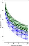 |
Fig. 4 Average radial profiles of the Hα surface brightness stacked according to specific AGN candidates. The shaded regions correspond to the 16th and 84th percentiles of each stacked radial profile. The solid green line corresponds to the AGN selected using a 2 kpc circular aperture, and its shaded area is filled with hollow circles. The black dash-dot line corresponds to the AGN selected by an aperture of 10 kpc, and its shaded area is filled with dots. Finally, the blue dashed line corresponds to the AGN selected by the 10 kpc aperture but excludes the AGN selected by the 2 kpc aperture. The last line has a shaded area filled with hollow squares. |
4.2 Classifications based on a 3″and 2 kpc aperture
Many current and early surveys have studied the general properties of galaxies based on single fiber 2″ (e.g., Dawson et al. 2013) or 3″ apertures (e.g., Gunn et al. 2006). Consequently, AGN identifications have frequently been made - especially for galaxies observed within SDSS surveys – based on measurements in these apertures. For MaNGA, for example, key AGN work has been done by classifying AGN using optical diagnostics on a 3″ aperture (Rembold et al. 2017; Sánchez et al. 2018). We therefore select the same aperture (3″) to study the impact of low-redshift optically selected AGN candidates when compared to a kpc-based aperture catalog. Our kpc-based aperture is used with the intention of reducing aperture effects (given by the redshift range of MaNGA galaxies) on selected AGN candidates and to focus on the compact AGN region.
AGN can ionize the gas in host galaxies up to kpc scales. This is commonly referred to as the narrow-line region (NLR; see Netzer 2015). The typical sizes of NLRs have been studied in recent decades (e.g., Bennert et al. 2006; Chen et al. 2011; Netzer 2015; Padovani et al. 2017), with a consensus being formed as to a lower limit of between hundreds of parsecs (pc) up to ~1 kpc in radius. Therefore, the ionizing source of some AGN can be easily diluted even at small apertures.
We note that the smaller the aperture, the more galaxies are classified as AGN (see Fig. 2). Specifically, we find that 59 AGN candidates from the 0.5 kpc catalog are not classified as AGN in the 2 kpc catalog. The median redshift of these 59 galaxies is 0.032, while the median redshift of the AGN population at 2 kpc is 0.045. This corresponds to a median resolution of 1.05 kpc and 1.58 kpc, respectively3. Indeed, this suggests that the NLR sizes of these 59 AGN candidates (if indeed proven to be true AGN) are small enough to be unresolved by the MaNGA survey and these objects are therefore missed when using a 2 kpc aperture. If we perform the same comparison between the 2 kpc and 5 kpc catalogs, we find that 122 galaxies are not classified as AGN in the 5 kpc catalog. The median resolution of these 122 galaxies is 1.12 kpc and the median resolution of the AGN population in the 5 kpc catalog is 1.60 kpc. When we carry out such comparisons now using the arcsecond-based or effective radius-based apertures, we find that the galaxies that are not classified as AGN in larger apertures still have a similar median kpc resolution to those at smaller apertures. We interpret this as a clear suggestion that the kpc-based aperture is more consistent with the physical properties of AGN.
Furthermore, MaNGA samples can achieve a median spatial resolution of about 1.37 kpc (Wake et al. 2017). This spatial resolution and the suggested physical sizes of the NLR motivate us to use an aperture of 2 kpc in diameter. To carry out a comparison between catalogs based on different apertures (see Sect. 5), we choose the following four catalogs:
circular aperture with a 2 kpc diameter using full BPT diagnostics ([NII]/Hα, [SII]/Hα, [OI]/Hα);
circular aperture with a 2 kpc diameter excluding the [OI]/Hα BPT diagnostic;
square aperture with a 3″ size on the side using full BPT diagrams ([NII]/Hα, [SII]/Hα, [OI]/Hα);
square aperture with a 3″ size excluding the [OI]/Hα BPT diagnostic.
We compute each AGN catalog following the procedure described in Sect. 3.2 including the EW(Hα) cut. The full classification and the number of galaxies corresponding to each class (star-forming, Seyfert, LINER, composite, and ambiguous, and the final AGN candidates) for these apertures are shown in Tables 1 and 2, as is the total number of galaxies used in that BPT classification. In these tables, we also report the number of galaxies that the different selections have in common.
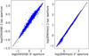 |
Fig. 5 Comparison of EW(Hα) and [OIII]/Hβ measurements derived from an aperture of 2 kpc and 3″ × 3″, respectively. Filled blue circles correspond to a comparison between measurements of EW(Hα) (right-hand plot) and [OШ]/Hβ ratio (left-hand plot) from our 2 kpc aperture (y-axis) and 3″ × 3″ aperture (x-axis). The measurements shown here correspond to the full MaNGA sample. The solid black line in both plots shows the one-to-one ratio that the values should follow if they have the same value. |
4.3 Hosts of emission-line galaxies
The number of successfully BPT-classified galaxies is an increasing number of decreasing S/N cuts. The BPT classification becomes more biased towards less massive galaxies (Brinchmann et al. 2004) as the S/N cut increases (see below). To present the impact of using our S/N limit (S/N > 3), in Fig. 6, we show the mass distribution (top histogram) and star formation rate (right-hand histogram) of the classified and unclassified galaxies. We use the stellar masses and star formation rates derived from the PIPE3D. In particular, the star formation rate in each galaxy is estimated with the dust-corrected Hα luminosity using the relationship proposed by Kennicutt (1998). This measurement should be treated as an upper limit since the PIPE3D uses the integrated Hα flux, which could include contamination of regions where the ionization source is not related to recent star formation events (see Sánchez et al. 2022). We note that our classification is biased towards higher star formation rates and lower stellar masses. This is an expected (and known) caveat given that optical emission lines are sensitive to the ongoing star formation in galaxies (Kewley & Ellison 2008). High-energy photons produced by young and hot stars are able to produce powerful emission lines through ionization (Kewley et al. 2001). However, galaxies whose stellar population is dominated by old stars are not generally able to produce the strong emission lines needed for typical optical classifications (e.g., satisfying S/N-specific criteria). Indeed, Kauffmann et al. (2003b) find that SDSS galaxies with higher masses present older stellar populations and that the fraction of high-mass galaxies with recent star formation is lower than in less massive galaxies. We further discuss how this impacts our AGN selection in Sect. 4.4.
We find very little or no change in the stellar-mass distribution of the AGN candidates when selecting them by the different aperture steps, regardless of the unit used (kpc, arcsec, or Reff). The typical stellar-mass distribution has a median of ~1011 M⊙. Despite the similarity in their stellar-mass distributions, we do not expect an accurate AGN BPT selection when using larger apertures. This similarity can occur due to the presence of a population of galaxies with DIG-dominated regions, whose properties can mimic AGN-like signatures (these galaxies are also massive, but older; see Sect. 4.1).
The star formation rate (derived from the integrated Hα flux) distribution from AGN selected using small apertures is also in agreement for AGN selected at large apertures, selecting very low SFR(Hα) populations at very large apertures. Our AGN candidates (using our 2 kpc catalog) follow an offset lying mostly below the star-formation main sequence (SFMS; see Fig. 7) and above the retired galaxies sequence (RGS). Our AGN candidates are located mostly in the green valley region (Salim 2014). Leslie et al. (2016) used optical diagnostics classification and found that Seyfert-classified galaxies (with z < 0.1) lie mostly below the SFMS. Schawinski et al. (2009) find similar results using a sample of obscured and unobscured AGN, concluding that their AGN host galaxies (0.01 < z < 0.07) are more likely to be found in the green valley. Similar results have been discussed in a sample with higher redshifts (z < 2.0; Pović et al. 2012), suggesting that these AGN could be part of a transitional phase, driving star-forming galaxies into a more quiescent phase. Indeed, further evidence has been found by Le Fèvre et al. (2019) in even higher redshift ranges (2 < z < 3.8), where strong C III] emitters (consistent with AGN sources) are more likely to be found below the SFMS (with an increasing outflow velocity in the strongest C III] emitters), suggesting that negative feedback quenches star-forming galaxies into a quiescent population. We will further discuss the outflow properties in MaNGA-AGN-selected galaxies in an upcoming publication (Albán et al., in prep.).
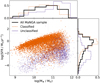 |
Fig. 6 Stellar mass vs. star formation rate (derived from Hα) extracted from the Pipe3D (Sánchez et al. 2016) value-added catalog. We color each target in orange or purple on the scatterplot to show whether or not, respectively, that specific galaxy was considered in the BPT classification scheme (meaning that it met our S/N criteria specified in Sect. 3.1). This plot is based on the classification using a 2 kpc aperture without considering the [O I] BPT diagram. The histograms show the distributions of stellar mass (top) and star formation rate (right). Distributions for the BPT classified and unclassified galaxies correspond to the dashed and solid histograms, respectively. The distribution of the whole MaNGA sample is shown in the black bold histogram. The distributions of the histograms are normalized, and the y-axis in the histograms corresponds to the normalized counts. |
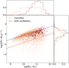 |
Fig. 7 Similar to Fig. 6, but we focus here on the BPT-classified sample (orange), highlighting the AGN candidates (dark red) selected from a 2 kpc aperture (see Sect. 3.2). We show the SFMS and the RGS from Cano-Díaz et al. (2016) using blue and red dashed lines, respectively. |
4.4 Hosts with very low S/N or no emission lines
We find that the unclassified galaxies (with S/N < 3 criteria) are typically more massive and have lower star formation rates (see Fig. 6) than galaxies with higher S/N. This is an expected behavior (e.g., Brinchmann et al. 2004), which results from the fact that these galaxies are dominated by old stellar populations and have low cold gas fractions (Wylezalek et al. 2022). For example, Brinchmann et al. (2004) found (in a sample of SDSS galaxies) that the flux of the [O III]λ5008 emission line decreases with stellar mass, with objects thus showing typically lower S/N (consistent with the discussion in Sect. 4.3). This trend is vice versa for the very high-mass galaxies due to the prevalence of AGN at these stellar masses (seen in Kauffmann et al. 2003a).
Using our 2 kpc aperture classification, we take the 4000 Å (D4000) break as a proxy of stellar age (Kauffmann et al. 2003a,b). While the MaNGA sample and our classified targets have a median D4000 value of ~1.36 and ~1.46, respectively, our unclassified sample of galaxies is typically older, with a median of D4000 ~ 1.71 and with very low EW(Hα) with a median of ~0.22 Å. We also find that these galaxies typically occupy the Green Valley and Quiescent region on the D4000 versus stellar mass diagram. Thus, we typically exclude old and high-stellar-mass galaxies with low star-formation rates. A fraction of these discarded galaxies are classified by Comerford et al. (2020) as AGN through radio-selection methods, and the authors discuss the radio-mode AGN as a possible final phase in the AGN evolution.
In a very early release of the MaNGA survey, Belfiore et al. (2016) used 646 galaxies to study the spatially resolved BPT diagrams, focusing on low ionization emission-line region (LIER) galaxies. These authors propose a classification scheme where 151 galaxies had spaxels with a very low S/N in the emission lines or no emission lines at all. They use the spaxels of all the galaxies that were not able to be classified and compute their EW(Hα), finding a median of 0.5 Å. For our unclassified sources, we also compute the median EW(Hα) from the central spaxel as well as the entire footprint, finding that the values do not exceed 0.4 Å. This median EW(Hα) is consistent with Belfiore et al., who classify lineless galaxies as the ones with EW(Hα) < 1.0 Å within one effective radius. Our AGN selection, by default, excludes the galaxies whose aperture-averaged EW(Hα) is lower than 3 Å. We therefore do not expect a significant contribution of AGN candidates (based on our selection algorithm) coming from galaxies with no emission lines due to our S/N cut.
5 Comparison between AGN catalogs
To test our classification catalogs, in this section we aim to study the impact of aperture size (2 kpc and 3″ specifically in this section) on the final AGN classification. We also explore the reasons for the discrepancies and/or cross-matches between reported catalogs from the literature (described in Sect. 2) and our classification described in Sect. 3. When comparing our catalogs to those from the literature, we restrict our catalogs to match the corresponding MaNGA sample (e.g., if an AGN selection was made using the MPL5 sample, we only use our AGN selected from that specific subsample).
5.1 Internal comparison of our catalogs
As seen in Tables 1 and 2 (see also Fig. 2), the total number of classified galaxies (after the S/N criteria) is greater when using a 3″ × 3″ aperture than the 2 kpc aperture. The latter is not surprising, given that more than half of the sample has a redshift that causes the aperture of 3″ to correspond to physical sizes of greater than 2 kpc. This means that for an aperture of 3″ × 3″ in this sample, more pixels are considered, increasing the chance of meeting our S/N criteria.
Even though there are more classifiable targets in the 3″ × 3″ aperture catalog, fewer targets are selected as AGN by the 3″ × 3″ aperture. Using only the [N II]/Hα and [S II]/Hα BPT diagrams, we identify 41 galaxies that are selected to be AGN based on the 2 kpc aperture but not by the 3″ × 3″ aperture. We show these galaxies in Fig. 8, revealing the impact on the BPT distribution when using the kpc-based versus the arcsecond-based aperture. The most common reason for this disagreement is that the (larger) 3″ × 3″ aperture pushes more targets to the star-forming regime. We observe that the lowest redshift galaxies are those that change position in the diagrams to the smallest extent, as the difference in physical size becomes more relevant at higher redshifts. We find that 11 out of these 41 galaxies no longer meet the EW(Hα) criterion (EW(Hα)>3Å).
If we reverse the comparison, we find that 21 galaxies are selected as AGN candidates based on the 3″ × 3″ aperture but not by the 2 kpc aperture. Most of them were not selected as AGN because they did not satisfy the EW(Hα) criteria: 11 of these did not satisfy the EW(Hα) cut, and the remaining ones were very close to the AGN division lines from the [N II] and [S II] BPT diagrams, and eight are classified as ambiguous, one as star-forming and one as a composite object in the 2 kpc aperture. Similar results are found when including the [O I]/Hα diagram in the selection algorithm, providing less AGN due to the typically low S/N in the [O I] emission line. We conclude that a 3″ -based aperture is more prone to shifting optically selected AGN galaxies (using a 2 kpc aperture) from the MaNGA survey towards a more star-forming appearance.
To quantify the dependence of the offset of the BPT classification on redshift, we focus on the [N II] BPT diagram and measure the distance between the BPT position of both kpc and 3″ apertures. We name this offset parameter Δ(NII), measured as follows:

where O3ap = [OIII]/Hβap and N2ap = |NII/Hαap, with ap the type of aperture used.
We display the distribution of Δ(NII), with ap1 = 2 kpc and ap2 = 3″, as a function of redshift in Fig. 9. The galaxies that are kicked in the direction of the HII-BPT region of the Nil BPT diagram are shown as purple squares. We use negative values (see the orange circles) to show the galaxies that are shifted toward the AGN region. The latter shows that the discrepancy between flux-ratio measurements (Eq. (2)) from a 2 kpc and a 3″ aperture in the NII-BPT diagram is more prone to increase, showing greater scatter at higher redshift. We see a greater concentration of galaxies moving towards a more HII-like region (purple squares) and fewer galaxies shifting towards an AGN-like classification (orange circles) for these optically AGN-selected galaxies. The empty symbols (squares or circles) show the AGN candidates selected in one aperture but not in the other. The empty squares (AGN in the 2 kpc aperture but excluded by the 3″ aperture) reveal that more AGN candidates are being excluded by the 3″ aperture, supporting our findings in Fig. 8. The discrepancies in this comparison are more prominent for more highly redshifted galaxies.
We also see that the impact of the aperture size remains almost negligible when the physical size of the arcsecond-based aperture matches the kpc aperture size, as expected. We show in dashed lines the circumscribed and inscribed square of a circle of radius 1 kpc, displaying the redshift range where the squared aperture mostly matches the circular-kpc-based aperture. Furthermore, we find no correlation between Δ(NII) and the axis ratio (b/a) when looking at our AGN candidates.
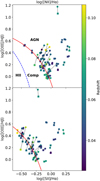 |
Fig. 8 BPT distribution for galaxies that were selected by the 2 kpc aperture (circles) but not by the 3″ × 3″ aperture (squares); each pair is connected by a black line. Both catalogs are performed as in Sect. 3.2, with the [OI]/Hα diagram being excluded. Each target is colored by its redshiſt. We plot the empirical division lines that will give each target a specific classification (e.g., AGN-like galaxy, composite object, or HII-star-forming galaxies): red lines correspond to Kewley et al. (2001), and the blue dashed line in the top plot corresponds to Kauffmann et al. (2003a). |
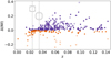 |
Fig. 9 Magnitude of the offset between the position of a 3″ and 2 kpc aperture in the [NII]–BPT diagram as a function of the redshift of the target. The data displayed in this plot correspond to the Δ(NII) from AGN-selected galaxies using a 2 kpc aperture (and excluding the [O I] BPT diagram). Orange solid circles correspond to galaxies whose offset slope points towards the AGN BPT region (outside the HII-BPT region). In contrast, the solid purple circles correspond to the opposite, moving galaxies towards a more star-forming appearance. Empty symbols (squares or circles) correspond to galaxies that were selected as AGN in one aperture but not in the other (e.g., the empty squares are exactly the same objects that are shown in Fig. 5, meaning that they were selected as AGN by the 2 kpc aperture but not for the 3″ aperture). The dashed vertical lines correspond to the redshift values where the squared arcsecond aperture corresponds to the circumscribed and inscribed square of a circle of radius 1 kpc. |
5.2 Comparison to the AGN catalog from Sánchez et al. (2018)
We compare the MaNGA AGN catalog published in Sánchez et al. (2018; which was made using the Pipe 3D output; see Sect. 2.2) to our 3″×3″ aperture catalog. In order to perform a consistent comparison, we use the same EW(Hα) criteria (i.e., adapting to EW(Hα) > 1.5 Å), following the procedure in Sect. 3.2 and using BPT diagnostics excluding the [O I]/Hα diagram. Almost all of the AGN selected by Sánchez et al. (2018) are also selected in our catalog. We find two AGN candidates with differing classifications: one due to a disagreement in position on the BPT diagram, and the other not meeting the EW(Hα) criteria (solid diamonds in Fig. 10). When considering the full BPT scheme, only one extra mismatch occurs, which is due to the lack of classifiable pixels (S/N > 3) in the [O I] flux (from the DAP). If we make the same comparison with our 2 kpc aperture catalog and use the full BPT scheme, five galaxies that are selected by Sánchez et al. (2018) are not selected by our catalog: two with no classifiable pixels in [O I], two not satisfying the EW(Hα) criteria, and one with an ambiguous BPT position.
However, there are more than 40 AGN candidates (if we compare to any of our four catalogs using EW(Hα) > 3 A; see Sect. 4.2) that were not selected by Sánchez et al. (2018), and more than 100 when we relax to EW(Hα) > 1.5 A. The latter is shown in Fig. 10, where we show our emission-line-ratio measurements and adapt to the EW(Hα) > 1.5 Å criteria of these latter authors. Visual inspection suggests that many AGN candidates from our catalog that are not selected by Sánchez et al. (2018) are relatively close to the Kewley et al. (2001) demarcation line (see Fig. 10). Discrepancies for these targets can be related to the quality cut that we make at S/N > 3 for each emission line measured by the DAP, which excludes the specific pixel from our procedure that shows slight flux-ratio changes from the ones measured by Sánchez et al. (2018). However, Sánchez et al. (2018) reported 302 galaxies above the AGN division line (Kewley et al. 2001; Kauffmann et al. 2003a), suggesting that the discrepancies for the galaxies far away from the demarcation lines on the AGN selection are mostly related to the EW(Hα) measurements. These discrepancies are a consequence of a different treatment of the stellar continuum when measuring EW(Hα) (already reported in Thomas et al. 2013; Wylezalek et al. 2018) and possibly due to the difference in the S/N cut criteria.
In Fig. 11, we compare the EW(Hα) measurements from the two AGN catalogs (left plot). A 1D polynomial suggests that the EW(Hα) measurements are mostly in agreement. However, the one-to-one comparison of the EW(Hα) values shows important scatter. At lower EW(Hα)s, our measurements (from our 3″ procedure) predict typically larger values than those measured by Sánchez et al. (2018). This supports the idea that the main discrepancy in the AGN selection comes from the differences between the EW(Hα) values. In the right-hand plot, we compare the [O III]/Hα ratio measurements. In our catalog, [O III]/Hα has typically greater values (also reported in Belfiore et al. 2019, when comparing the DAP measurements to Pipe 3D, and reportedly due to a different choice of stellar continuum treatments).
The latter is expected because there is better agreement in the AGN selection before applying the EW(Hα) criteria.
A minor extra consideration that could drive the discrepancy is that we are weighting pixels according to their enclosed fraction with their selected aperture (see Sect. 3.2), which we do not expect to have a significant impact. We find similar results when using our 2 kpc aperture and the EW(Hα) = 1.5 Å criteria.
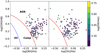 |
Fig. 10 BPT position of all the AGN candidates that are in disagreement between our 3″ aperture catalog (without [OI]/Hα BPT diagram) and the catalog from Sánchez et al. (2016). Solid circles correspond to targets selected by our catalog but not by these latter authors. Solid diamonds correspond to the opposite situation (AGN-selected by Sánchez et al. 2016, but not by our catalog). The color on the scatter plots corresponds to the logarithmic EW(Hα). The red lines and the blue dashed line on the left plot correspond to Kewley et al. (2001) and Kauffmann et al. (2003a), respectively. |
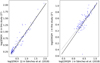 |
Fig. 11 Comparison between measurements of EW(Hα) values (left-hand plot) and [OIII]Hβ ratios (right-hand plot) from this work (y-axis; using a 3″ aperture) and Sánchez et al. (2018, x-axis) in a logarithmic scale. The measurements (in blue circles) shown here correspond to the AGN-candidate subsample from Sánchez et al. (2018) The solid black line in both plots shows the one-to-one ratio that the values should follow if they have the same value. The gray dashed line in the plots shows a 1D polynomial fit to the distribution. |
5.3 Comparison to the AGN catalog from Rembold et al. (2017)
Using our 3″ × 3″ aperture and excluding the [O I]/Hα BPT diagram, we find that only one target that does not cross-match with the AGN candidates from Rembold et al. (2017). However, 14 galaxies drop from the cross-match when we adapt to the EW(Hα) > 3 Å criteria. We display the mismatched targets in Fig. 12 and we force the contrast of the EW(Hα) color bar to have its maximum value at EW(Hα) = 3 (in logarithmic scale) in order to better distinguish why these galaxies were not classified as AGN in our procedure in terms of the EW(Hα). Furthermore, if we consider the full BPT scheme (including the [O I]/Hα BPT), the latter behavior holds. When we perform the same comparison with our absolute 2 kpc aperture, we find one more crossmatched target. When reversing the comparison, around 36 targets were selected by our catalog but not by the Rembold catalog.
Including the [OI]-based BPT diagnostic or changing the aperture (between 3″ × 3″ arcsec or 2 kpc) does not seem to impact the number of AGN-selected sources, as also found in the comparison with the Sánchez et al. (2018). classification. Five targets are not classified as AGN candidates (but as ambiguous) because they fall into the star-forming regime in the [S II/Hα] diagram. Most of the extra AGN candidates from Rembold et al. (2017) do not satisfy the EW(Hα) > 3 Å criteria. Specifically, the 14 and the further 36 discrepancies (see Fig. 12) suggest that a S/N cut plays an important role in the EW(Hα) criteria, because we use a S/N > 3. Low-S/N spaxels could be biased by low EW(Hα) values as this quantity is measured by the ratio between the emission-line and continuum fluxes (Thomas et al. 2013). An important discrepancy comes from the difference in the stellar subtraction from MaStar (MaNGA Stellar Library) when measuring emission lines (Yan et al. 2019). A smaller impact might be related to the way in which we measure the flux (see Fig. 1).
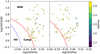 |
Fig. 12 BPT distribution of all the AGN candidates that are in disagreement between our 3″ aperture and BPT excluding [OI]/Hα diagram catalog and the catalog from Rembold et al. (2017). Solid circles correspond to targets selected by our catalog, but not by these latter authors. Solid diamonds correspond to the opposite (selected by Rembold et al. 2017 but not by our catalog). The color on the scatter plots corresponds to a specific EW(Hα) range width whose contrast is forced to be within 1.0 Å > EW(Hα) > 3.0 A in order to emphasize which targets satisfied the EW(Hα) > 3.0 A condition. The red lines correspond to Kewley et al. (2001) and the blue dashed line on the left plot corresponds to Kauffmann et al. (2003a). |
5.4 Comparison to the AGN catalog from Wylezalek et al. (2018)
An interesting finding from the comparisons conducted above is that, as we increase the aperture (either using a kpc or arcsecond aperture), our catalogs have fewer AGN in common compared to the catalogs of Sánchez et al. (2018) and Rembold et al. (2017). However, the agreement between our catalogs and that of Wylezalek et al. (2018) remains almost constant as we increase the aperture for the selection, with a small increase at greater apertures.
In contrast to the previous comparisons, we find a greater disagreement between our AGN candidates and the ones from Wylezalek et al. (2018). In Wylezalek et al. (2018), the authors search for AGN signatures at all galactocentric distances. If we use our 2 kpc diameter aperture catalog (excluding [O I]/Hα), we find only 56 targets in agreement (Fig. 13). Changing between a 2 kpc or a 3″ aperture and the full BPT scheme has no relevant impact on this comparison. The discrepancies reported in this comparison are mostly related to the significant differences in the selection methods. The method of Wylezalek et al. (2018) does not use defined apertures, but pixel fractions (e.g., if a relevant fraction of pixels is classified as AGN); every pixel is used, whether it is near to or far from the center of the galaxy. Wylezalek et al. (2018) argue that using the full power of spatially resolved spectra reveals possibly hidden and/or weaker AGN candidates that may have been missed due to obscuring effects, recently turned-off AGN, or AGN that are not located in the reported center of the MaNGA NSA catalog (due to mergers or off-set AGN).
5.5 Comparison to the multiwavelength AGN catalog from Comerford et al. (2020)
From their 406 AGN-selected galaxies, we find only 73 and 69 galaxies in agreement from our 2 kpc and 3″ (excluding [O I]/Hα) AGN catalog, respectively, when compared to the multiwavelength AGN catalog from Comerford et al. (2020, for a description of this catalog; see Sect. 2.5). These numbers decrease as we increase the size of our apertures. Better agreement is found when we relax the EW(Hα) criteria. Because of our S/N cut, our 2 kpc aperture catalog was unable to classify around 100 galaxies that were classified as AGN by Comerford et al. (2020). Figure 14 displays the BPT diagrams highlighting the multiwavelength-classified AGN from the Comerford et al. (2020) catalog. The emission-line ratios of the AGN sample of Comerford et al. (2020) do not gather where our optical AGN-selected population is. This highlights the fact that not all AGN can be classified using optical emission line diagnostics, revealing the known caveats of BPT selection.
 |
Fig. 13 AGN candidates that are in the Wylezalek et al. (2018) catalog but are excluded by our AGN selection (solid diamonds) using a 2 kpc aperture without the [O I]/Hα BPT criteria with EW(Hα) > 3 A (with the contrast forced as in Fig. 12). The candidates that were selected by our procedure but not by Wylezalek et al. (2018) are shown as filled circles. The dashed and solid lines show the same information as described in Fig. 8. |
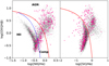 |
Fig. 14 Our MaNGA BPT classification using a 2 kpc aperture. We highlight the multiwavelength (based on radio, IR, broad-line, and X-ray selection methods; see Sect. 2.5)-selected AGN candidates from Comerford et al. (2020) with pink star-like symbols. |
6 Conclusions
We used the final data release (DR17) of the SDSS-MaNGA survey (10010 galaxies) to classify galaxies based on their BPT diagnostics. We created catalogs using a range of apertures (in units of kpc, arcsecond, and effective radius) as the basis of our classification. In each aperture, we measure the BPT diagnostics and include an EW(Hα) cut for the final AGN classification. We studied how galaxies can change classification as we increase the aperture used for their characterization. Our main results are as follows:
MaNGA AGN candidates for small (< 6 kpc) kpc-based apertures lie below the SFMS (see Fig. 7), in agreement with previous results (e.g., Sánchez et al. 2018; Comerford et al. 2020). These AGN candidates are massive with stellar mass of around ~ 1011 M⊙ and a median Hα-derived star formation rate of ~1.44 M⊙ yr−1.
We show that the number of galaxies classified as AGN decreases with increasing aperture size up to ~ 6 kpc, 6″ or 1.2 Reff, depending on the units used, respectively. We argue that this is due to the compact nature of the AGN phenomenon. As the aperture size increases, one gets closer to capturing the entire spectrum of a galaxy, potentially reducing the dominance of AGN emission and positioning the observed galaxies towards the composite or star-forming region.
Intriguingly, at apertures greater than 6 kpc, 6″ or 1.2 Reff), the trend reverses and the number of galaxies classified as AGN starts to increase (see Fig. 2). The stacked radial cumulative surface-brightness profiles for the AGN candidates that are only found in very large apertures (but not in the smaller ones) show very low Hα surface brightness (see Fig. 4). This is consistent with AGN selection being strongly contaminated by the effect of DIG-dominated regions. This implies that using a very large aperture selects fewer true AGN.
When we compare our catalog with MaNGA AGN aperture-based catalogs from the literature (using previous data releases) we find the following important parameter. In addition to the classical BPT line ratios, the measurement of the EW(Hα) is a commonly used and important additional diagnostic. In our comparisons, we show that different treatments to fit the stellar continuum have a strong impact on the faint AGN population. This is because EW(Hα) measurements are sensitive to small changes of the continuum model. An AGN selection based on optical diagnostics can therefore vary greatly between different analyses (see Figs. 10–12). Additional discrepancies in the selection of AGN candidates are related to the strong differences in the selection criteria (see Sect. 2.4 and Fig. 13) and the choice of the observed wavelength range when classifying galaxies (see Sect. 2.5 and Fig. 14).
With this work, we show that the choice of aperture size impacts optical AGN selection and galaxy classification. In comparison to single-fiber optical galaxy classification, IFU observations offer a more complete characterization of the origin of ionizing sources in galaxies (e.g., identifying DIG regions) and allow one to minimize aperture effects (e.g., using a redshift-independent aperture), thereby reducing the bias in AGN-selection techniques.
Acknowledgements
D.W. acknowledges support through an Emmy Noether Grant of the German Research Foundation, a stipend by the Daimler and Benz Foundation and a Verbundforschung grant by the German Space Agency. Funding for the Sloan Digital Sky Survey IV has been provided by the Alfred P. Sloan Foundation, the US Department of Energy Office of Science, and the Participating Institutions. SDSS-IV acknowledges support and resources from the Center for High Performance Computing at the University of Utah. The SDSS web site is www.sdss.org. SDSS-IV is managed by the Astro-physical Research Consortium for the Participating Institutions of the SDSS Collaboration including the Brazilian Participation Group, the Carnegie Institution for Science, Carnegie Mellon University, the Chilean Participation Group, the French Participation Group, Harvard-Smithsonian Center for Astrophysics, Instituto de Astrofísica de Canarias, The Johns Hopkins University, Kavli Institute for the Physics and Mathematics of the Universe (IPMU) / University of Tokyo, the Korean Participation Group, Lawrence Berkeley National Laboratory, Leibniz Institut für Astrophysik Potsdam (AIP), Max-Planck-Institut für Astronomie (MPIA Heidelberg), Max-Planck-Institut für Astrophysik (MPA Garching), Max-Planck-Institut für Extraterrestrische Physik (MPE), National Astronomical Observatories of China, New Mexico State University, New York University, University of Notre Dame, Observatario Nacional / MCTI, The Ohio State University, Pennsylvania State University, Shanghai Astronomical Observatory, United Kingdom Participation Group, Universidad Nacional Autonoma de México, University of Arizona, University of Colorado Boulder, University of Oxford, University of Portsmouth, University of Utah, University of Virginia.
References
- Abdurro’uf, Accetta, K., Aerts, C., et al. 2022, ApJS, 259, 35 [NASA ADS] [CrossRef] [Google Scholar]
- Abolfathi, B., Aguado, D. S., Aguilar, G., et al. 2018, ApJS, 235, 42 [NASA ADS] [CrossRef] [Google Scholar]
- Alexander, D., & Hickox, R. 2012, New Astron. Rev., 56, 93 [CrossRef] [Google Scholar]
- Allen, M. G., Groves, B. A., Dopita, M. A., Sutherland, R. S., & Kewley, L. J. 2008, ApJS, 178, 20 [Google Scholar]
- Antonucci, R. 1993, ARA&A, 31, 473 [Google Scholar]
- Azadi, M., Coil, A. L., Aird, J., et al. 2017, ApJ, 835, 27 [NASA ADS] [CrossRef] [Google Scholar]
- Baldwin, J. A., Phillips, M. M., & Terlevich, R. 1981, PASP, 93, 5 [Google Scholar]
- Barthelmy, S. D., Barbier, L. M., Cummings, J. R., et al. 2005, Space Sci. Rev., 120, 143 [Google Scholar]
- Becker, R. H., White, R. L., & Helfand, D. J. 1995, ApJ, 450, 559 [Google Scholar]
- Beifiori, A., Courteau, S., Corsini, E. M., & Zhu, Y. 2011, MNRAS, 419, 2497 [Google Scholar]
- Belfiore, F., Maiolino, R., Maraston, C., et al. 2016, MNRAS, 461, 3111 [Google Scholar]
- Belfiore, F., Westfall, K. B., Schaefer, A., et al. 2019, AJ, 158, 160 [CrossRef] [Google Scholar]
- Bennert, N., Jungwiert, B., Komossa, S., Haas, M., & Chini, R. 2006, A&A, 456, 953 [NASA ADS] [CrossRef] [EDP Sciences] [Google Scholar]
- Bershady, M. A., Verheijen, M. A. W., Swaters, R. A., et al. 2010, ApJ, 716, 198 [NASA ADS] [CrossRef] [Google Scholar]
- Bessiere, P. S., & Almeida, C. R. 2022, MNRAS, 512, L54 [NASA ADS] [CrossRef] [Google Scholar]
- Binette, L., Magris, C. G., Stasinska, G., & Bruzual, A. G. 1994, A&A, 292, 13 [NASA ADS] [Google Scholar]
- Brinchmann, J., Charlot, S., White, S. D. M., et al. 2004, MNRAS, 351, 1151 [Google Scholar]
- Buchner, J., Treister, E., Bauer, F. E., Sartori, L. F., & Schawinski, K. 2019, ApJ, 874, 117 [NASA ADS] [CrossRef] [Google Scholar]
- Bundy, K., Bershady, M. A., Law, D. R., et al. 2015, ApJ, 798, 7 [Google Scholar]
- Cano-Díaz, M., Maiolino, R., Marconi, A., et al. 2012, A&A, 537, A8 [Google Scholar]
- Cano-Díaz, M., Sánchez, S. F., Zibetti, S., et al. 2016, ApJ, 821, L26 [Google Scholar]
- Chen, Z.-F., Qin, Y. P., Chen, Z. Y., & Lü, L. Z. 2011, JApA, 32, 273 [NASA ADS] [Google Scholar]
- Cid Fernandes, R., Stasińska, G., Schlickmann, M. S., et al. 2010, MNRAS, 403, 1036 [Google Scholar]
- Comerford, J. M., Negus, J., Müller-Sánchez, F., et al. 2020, ApJ, 901, 159 [NASA ADS] [CrossRef] [Google Scholar]
- Condon, J. J., Cotton, W. D., Greisen, E. W., et al. 1998, AJ, 115, 1693 [Google Scholar]
- Dawson, K. S., Schlegel, D. J., Ahn, C. P., et al. 2013, AJ, 145, 10 [Google Scholar]
- Decarli, R., Gavazzi, G., Arosio, I., et al. 2007, MNRAS, 381, 136 [NASA ADS] [CrossRef] [Google Scholar]
- Dopita, M. A., Kewley, L. J., & Sutherland, R. S. 2002, Rev. Mex. Astron. Astrofis. Conf. Ser., 12, 225 [NASA ADS] [Google Scholar]
- Drory, N., MacDonald, N., Bershady, M. A., et al. 2015, AJ, 149, 77 [CrossRef] [Google Scholar]
- Dugan, Z., Gaibler, V., Bieri, R., Silk, J., & Rahman, M. 2017, ApJ, 839, 103 [NASA ADS] [CrossRef] [Google Scholar]
- Fabian, A. 2012, ARA&A, 50, 455 [CrossRef] [Google Scholar]
- Ferland, G. J., & Netzer, H. 1983, ApJ, 264, 105 [NASA ADS] [CrossRef] [Google Scholar]
- Ferrarese, L. & Merritt, D. 2000, ApJ, 539, L9 [NASA ADS] [CrossRef] [Google Scholar]
- Gómez, P. L., Nichol, R. C., Miller, C. J., et al. 2003, ApJ, 584, 210 [Google Scholar]
- Graham, A. W. 2016, Galactic Bulges, eds. E. Laurikainen, R. F. Peletier, & D. A. Gadotti (Springer), 263 [NASA ADS] [CrossRef] [Google Scholar]
- Groves, B. A., Dopita, M. A., & Sutherland, R. S. 2004, ApJS, 153, 75 [NASA ADS] [CrossRef] [Google Scholar]
- Gültekin, K., Richstone, D. O., Gebhardt, K., et al. 2009, ApJ, 698, 198 [Google Scholar]
- Gunn, J. E., Siegmund, W. A., Mannery, E. J., et al. 2006, AJ, 131, 2332 [NASA ADS] [CrossRef] [Google Scholar]
- Haffner, L. M., Dettmar, R.-J., Beckman, J. E., et al. 2009, Rev. Mod. Phys., 81, 969 [CrossRef] [Google Scholar]
- Halpern, J. P., & Steiner, J. E. 1983, ApJ, 269, L37 [CrossRef] [Google Scholar]
- Harrison, C. 2014, Ph.D. Thesis, Durham University, UK [Google Scholar]
- Heckman, T. M., & Best, P. N. 2014, ARA&A, 52, 589 [Google Scholar]
- Hirschmann, M., Charlot, S., Feltre, A., et al. 2017, MNRAS, 472, 2468 [NASA ADS] [CrossRef] [Google Scholar]
- Ho, L. C. 2008, ARA&A, 46, 475 [Google Scholar]
- Hopkins, A. M., Miller, C. J., Nichol, R. C., et al. 2003, ApJ, 599, 971 [Google Scholar]
- Hoyle, F., & Ellis, G. R. A. 1963, Austr. J. Phys., 16, 1 [NASA ADS] [CrossRef] [Google Scholar]
- Iglesias-Páramo, J., Vílchez, J. M., Rosales-Ortega, F. F., et al. 2016, ApJ, 826, 71 [Google Scholar]
- Jones, A., Kauffmann, G., D’Souza, R., et al. 2017, A&A, 599, A141 [NASA ADS] [CrossRef] [EDP Sciences] [Google Scholar]
- Kauffmann, G., Heckman, T. M., Tremonti, C., et al. 2003a, MNRAS, 346, 1055 [Google Scholar]
- Kauffmann, G., Heckman, T. M., White, S. D. M., et al. 2003b, MNRAS, 341, 33 [Google Scholar]
- Keel, W. C., Maksym, W. P., Bennert, V. N., et al. 2015, AJ, 149, 155 [NASA ADS] [CrossRef] [Google Scholar]
- Kennicutt, R. C., Jr. 1992, ApJ, 388, 310 [CrossRef] [Google Scholar]
- Kennicutt, R. C., Jr. 1998, ApJ, 498, 541 [Google Scholar]
- Kewley, L. J., & Ellison, S. L. 2008, ApJ, 681, 1183 [Google Scholar]
- Kewley, L. J., Dopita, M. A., Sutherland, R. S., Heisler, C. A., & Trevena, J. 2001, ApJ, 556, 121 [Google Scholar]
- Kewley, L., Jansen, R., & Geller, M. 2005, PASP, 117, 227 [NASA ADS] [CrossRef] [Google Scholar]
- Kewley, L. J., Groves, B., Kauffmann, G., & Heckman, T. 2006, MNRAS, 372, 961 [Google Scholar]
- Kewley, L. J., Dopita, M. A., Leitherer, C., et al. 2013, ApJ, 774, 100 [NASA ADS] [CrossRef] [Google Scholar]
- Kewley, L. J., Nicholls, D. C., & Sutherland, R. S. 2019, ARA&A, 57, 511 [Google Scholar]
- Kormendy, J., & Ho, L. C. 2013, ARA&A, 51, 511 [Google Scholar]
- Krishnarao, D., Benjamin, R. A., & Haffner, L. M. 2020, Sci. Adv., 6, eaay9711 [CrossRef] [Google Scholar]
- Law, D. R., Yan, R., Bershady, M. A., et al. 2015, AJ, 150, 19 [CrossRef] [Google Scholar]
- Law, D. R., Cherinka, B., Yan, R., et al. 2016, AJ, 152, 83 [Google Scholar]
- Le Fèvre, O., Lemaux, B. C., Nakajima, K., et al. 2019, A&A, 625, A51 [NASA ADS] [CrossRef] [EDP Sciences] [Google Scholar]
- Leslie, S. K., Kewley, L. J., Sanders, D. B., & Lee, N. 2016, MNRAS, 455, L82 [NASA ADS] [CrossRef] [Google Scholar]
- Mahoro, A., Pović, M., & Nkundabakura, P. 2017, MNRAS, 471, 3226 [Google Scholar]
- Mannucci, F., Belfiore, F., Curti, M., et al. 2021, MNRAS, 508, 1582 [NASA ADS] [CrossRef] [Google Scholar]
- Maoz, D. 2007, MNRAS, 377, 1696 [CrossRef] [Google Scholar]
- Maragkoudakis, A., Zezas, A., Ashby, M. L. N., & Willner, S. P. 2014, MNRAS, 441, 2296 [NASA ADS] [CrossRef] [Google Scholar]
- Masegosa, J., Márquez, I., Ramirez, A., & González-Martín, O. 2011, A&A, 527, A23 [NASA ADS] [CrossRef] [EDP Sciences] [Google Scholar]
- Nesvadba, N. P. H., Bicknell, G. V., Mukherjee, D., & Wagner, A. Y. 2020, A&A, 639, A13 [Google Scholar]
- Netzer, H. 2015, ARA&A, 53, 365 [Google Scholar]
- Padovani, P., Alexander, D. M., Assef, R. J., et al. 2017, A&ARv, 25, 2 [Google Scholar]
- Park, D., Woo, J.-H., Bennert, V. N., et al. 2015, ApJ, 799, 164 [NASA ADS] [CrossRef] [Google Scholar]
- Peterson, B. 2006, The Broad-Line Region in Active Galactic Nuclei, eds. D. Alloin, R. Johnson, & P. Lira (Springer), 77 [Google Scholar]
- Pović, M., Sánchez-Portal, M., García, A. M. P., et al. 2012, A&A, 541, A118 [NASA ADS] [CrossRef] [EDP Sciences] [Google Scholar]
- Rand, R. J., Kulkarni, S. R., & Hester, J. J. 1990, ApJ, 352, L1 [NASA ADS] [CrossRef] [Google Scholar]
- Rees, M. J. 1984, ARA&A, 22, 471 [Google Scholar]
- Rembold, S. B., Shimoia, J. S., Storchi-Bergmann, T., et al. 2017, MNRAS, 472, 4382 [Google Scholar]
- Reynolds, R. J. 1984, ApJ, 282, 191 [NASA ADS] [CrossRef] [Google Scholar]
- Salim, S. 2014, Serb. Astron. J., 189, 1 [NASA ADS] [CrossRef] [Google Scholar]
- Sánchez, S. F., Pérez, E., Sánchez-Blázquez, P., et al. 2016, Rev. Mex. Astron. Astrofis., 52, 171 [Google Scholar]
- Sánchez, S. F., Avila-Reese, V., Hernandez-Toledo, H., et al. 2018, Rev. Mex. Astron. Astrofis., 54, 217 [Google Scholar]
- Sánchez, S. F., Barrera-Ballesteros, J. K., Lacerda, E., et al. 2022, ApJS, 262, 36 [CrossRef] [Google Scholar]
- Schawinski, K., Virani, S., Simmons, B., et al. 2009, ApJ, 692, L19 [NASA ADS] [CrossRef] [Google Scholar]
- Singh, R., van de Ven, G., Jahnke, K., et al. 2013, A&A, 558, A43 [NASA ADS] [CrossRef] [EDP Sciences] [Google Scholar]
- Singh, C. B., Kulasiri, N., North, M., & Garofalo, D. 2021, PASP, 133, 104101 [NASA ADS] [CrossRef] [Google Scholar]
- Smith, A., & Bromm, V. 2019, Contemp. Phys., 60, 111 [NASA ADS] [CrossRef] [Google Scholar]
- Somerville, R. S., & Davé, R. 2015, ARA&A, 53, 51 [Google Scholar]
- Springel, V., Di Matteo, T., & Hernquist, L. 2005, MNRAS, 361, 776 [Google Scholar]
- Taniguchi, Y., Shioya, Y., & Murayama, T. 2000, ApJ, 120, 1265 [Google Scholar]
- Thomas, D., Steele, O., Maraston, C., et al. 2013, MNRAS, 431, 1383 [NASA ADS] [CrossRef] [Google Scholar]
- Vale Asari, N., Couto, G. S., Cid Fernandes, R., et al. 2019, MNRAS, 489, 4721 [NASA ADS] [CrossRef] [Google Scholar]
- Veilleux, S., & Osterbrock, D. E. 1987, ApJS, 63, 295 [Google Scholar]
- Veilleux, S., Kim, D. C., Sanders, D. B., Mazzarella, J. M., & Soifer, B. T. 1995, ApJS, 98, 171 [NASA ADS] [CrossRef] [Google Scholar]
- Volonteri, M., Dubois, Y., Pichon, C., & Devriendt, J. 2016, MNRAS, 460, 2979 [Google Scholar]
- Wagner, A. Y., Bicknell, G. V., Umemura, M., Sutherland, R. S., & Silk, J. 2016, Astron. Nachr., 337, 167 [NASA ADS] [CrossRef] [Google Scholar]
- Wake, D. A., Bundy, K., Diamond-Stanic, A. M., et al. 2017, AJ, 154, 86 [Google Scholar]
- Westfall, K. B., Cappellari, M., Bershady, M. A., et al. 2019, AJ, 158, 231 [Google Scholar]
- Wright, E. L., Eisenhardt, P. R. M., Mainzer, A. K., et al. 2010, AJ, 140, 1868 [Google Scholar]
- Wylezalek, D., Zakamska, N. L., Greene, J. E., et al. 2018, MNRAS, 474, 1499 [NASA ADS] [CrossRef] [Google Scholar]
- Wylezalek, D., Flores, A. M., Zakamska, N. L., Greene, J. E., & Riffel, R. A. 2020, MNRAS, 492, 4680 [NASA ADS] [CrossRef] [Google Scholar]
- Wylezalek, D., Cicone, C., Belfiore, F., et al. 2022, MNRAS, 510, 3119 [CrossRef] [Google Scholar]
- Yan, R., & Blanton, M. R. 2012, ApJ, 747, 61 [NASA ADS] [CrossRef] [Google Scholar]
- Yan, R., Chen, Y., Lazarz, D., et al. 2019, ApJ, 883, 175 [Google Scholar]
- Yi, C., SiDan, Z., XingYu, Z., et al. 2022, RAA, submitted [arXiv:2202.04795] [Google Scholar]
- Zhang, K., Yan, R., Bundy, K., et al. 2016, MNRAS, 466, 3217 [Google Scholar]
We checked the stacking of cumulative and noncumulative radial profiles of Hα surface brightness (for AGN candidates). The negligible differences do not impact the discussion in this section. We focus on the cumulative contribution of this parameter, motivated by the aim to take into account the effects of an increasing aperture-based selection.
We can estimate the median spatial resolution of this AGN-candidate population using the spatial element relation δ ≈ 35z kpc (see Bundy et al. 2015).
All Tables
MaNGA-DR17 catalog for optical diagnostics classification excluding the [O I] BPT diagram using a 2 kpc and a 3″×3″ aperture.
MaNGA-DR17 catalog for optical diagnostics classification including the [O I] BPT diagram using a 2 kpc and a 3″×3″ aperture.
BPT classification (without using [O I]/Hα), AGN selection, emission-line ratios, and equivalent-width values for the MaNGA galaxies.
All Figures
|
Fig. 1 Example of our weighted pixel averaging. The left plot shows (target with plate-ifu: 8725-9102) the flux of the [OIII]λ5007 emission line. Pixels with S/N < 3 are masked. The black circle indicates the 2 kpc circular diameter aperture where we average the flux for the emission line ratios. The right plot shows a zoom onto the aperture region, showing the percentage of the pixel area captured by the aperture shown in black. We show the value in each pixel that corresponds to the weight of the pixel when we compute the average fluxes. |
| In the text | |
|
Fig. 2 Variation in AGN classification with different aperture sizes. The y-axis in the top plots and the bottom left plot shows the number of galaxies classified as AGN (solid blue line) selected based on different aperture sizes and using different units. The selection is made following the algorithm described in Sect. 3.2, excluding the [O I]/Hα BPT diagram. In the top left plot, the kiloparsec aperture increases in steps of 0.5 kpc (in diameter). In the top right plot, the arcsecond aperture increases in steps of 0.5″ (in diameter). In the bottom left plot, the effective radius aperture increases in steps of 0.1 Reff (in radius). The red (vertical-dashed) line in the top panels corresponds to the apertures used for the comparisons in Sect. 5. In the bottom right plot, we show how the flux ratios in one BPT diagram change as a function of the aperture. This is done for three individual galaxies illustrated with different symbols (see the legend for their corresponding MaNGA-IDs). Each symbol is filled with a specific color that corresponds to the size of its aperture. In the bottom right plot, we also include the empirical division lines that will give each target a specific classification (e.g., AGN-like galaxy, composite object, or HII-star forming galaxies): red lines correspond to Kewley et al. (2001), and the blue dashed line on the left plot corresponds to Kauffmann et al. (2003a). |
| In the text | |
|
Fig. 3 Number of galaxies (y-axis) identified by a specific BPT classification (see the legend to the top right of the plot) using different selection aperture sizes (in kpc, x-axis). Each value is colored according to the average Hα surface brightness (color bar) within a 2 kpc aperture. This classification is done excluding the [O I] BPT diagram. |
| In the text | |
|
Fig. 4 Average radial profiles of the Hα surface brightness stacked according to specific AGN candidates. The shaded regions correspond to the 16th and 84th percentiles of each stacked radial profile. The solid green line corresponds to the AGN selected using a 2 kpc circular aperture, and its shaded area is filled with hollow circles. The black dash-dot line corresponds to the AGN selected by an aperture of 10 kpc, and its shaded area is filled with dots. Finally, the blue dashed line corresponds to the AGN selected by the 10 kpc aperture but excludes the AGN selected by the 2 kpc aperture. The last line has a shaded area filled with hollow squares. |
| In the text | |
|
Fig. 5 Comparison of EW(Hα) and [OIII]/Hβ measurements derived from an aperture of 2 kpc and 3″ × 3″, respectively. Filled blue circles correspond to a comparison between measurements of EW(Hα) (right-hand plot) and [OШ]/Hβ ratio (left-hand plot) from our 2 kpc aperture (y-axis) and 3″ × 3″ aperture (x-axis). The measurements shown here correspond to the full MaNGA sample. The solid black line in both plots shows the one-to-one ratio that the values should follow if they have the same value. |
| In the text | |
|
Fig. 6 Stellar mass vs. star formation rate (derived from Hα) extracted from the Pipe3D (Sánchez et al. 2016) value-added catalog. We color each target in orange or purple on the scatterplot to show whether or not, respectively, that specific galaxy was considered in the BPT classification scheme (meaning that it met our S/N criteria specified in Sect. 3.1). This plot is based on the classification using a 2 kpc aperture without considering the [O I] BPT diagram. The histograms show the distributions of stellar mass (top) and star formation rate (right). Distributions for the BPT classified and unclassified galaxies correspond to the dashed and solid histograms, respectively. The distribution of the whole MaNGA sample is shown in the black bold histogram. The distributions of the histograms are normalized, and the y-axis in the histograms corresponds to the normalized counts. |
| In the text | |
|
Fig. 7 Similar to Fig. 6, but we focus here on the BPT-classified sample (orange), highlighting the AGN candidates (dark red) selected from a 2 kpc aperture (see Sect. 3.2). We show the SFMS and the RGS from Cano-Díaz et al. (2016) using blue and red dashed lines, respectively. |
| In the text | |
|
Fig. 8 BPT distribution for galaxies that were selected by the 2 kpc aperture (circles) but not by the 3″ × 3″ aperture (squares); each pair is connected by a black line. Both catalogs are performed as in Sect. 3.2, with the [OI]/Hα diagram being excluded. Each target is colored by its redshiſt. We plot the empirical division lines that will give each target a specific classification (e.g., AGN-like galaxy, composite object, or HII-star-forming galaxies): red lines correspond to Kewley et al. (2001), and the blue dashed line in the top plot corresponds to Kauffmann et al. (2003a). |
| In the text | |
|
Fig. 9 Magnitude of the offset between the position of a 3″ and 2 kpc aperture in the [NII]–BPT diagram as a function of the redshift of the target. The data displayed in this plot correspond to the Δ(NII) from AGN-selected galaxies using a 2 kpc aperture (and excluding the [O I] BPT diagram). Orange solid circles correspond to galaxies whose offset slope points towards the AGN BPT region (outside the HII-BPT region). In contrast, the solid purple circles correspond to the opposite, moving galaxies towards a more star-forming appearance. Empty symbols (squares or circles) correspond to galaxies that were selected as AGN in one aperture but not in the other (e.g., the empty squares are exactly the same objects that are shown in Fig. 5, meaning that they were selected as AGN by the 2 kpc aperture but not for the 3″ aperture). The dashed vertical lines correspond to the redshift values where the squared arcsecond aperture corresponds to the circumscribed and inscribed square of a circle of radius 1 kpc. |
| In the text | |
|
Fig. 10 BPT position of all the AGN candidates that are in disagreement between our 3″ aperture catalog (without [OI]/Hα BPT diagram) and the catalog from Sánchez et al. (2016). Solid circles correspond to targets selected by our catalog but not by these latter authors. Solid diamonds correspond to the opposite situation (AGN-selected by Sánchez et al. 2016, but not by our catalog). The color on the scatter plots corresponds to the logarithmic EW(Hα). The red lines and the blue dashed line on the left plot correspond to Kewley et al. (2001) and Kauffmann et al. (2003a), respectively. |
| In the text | |
|
Fig. 11 Comparison between measurements of EW(Hα) values (left-hand plot) and [OIII]Hβ ratios (right-hand plot) from this work (y-axis; using a 3″ aperture) and Sánchez et al. (2018, x-axis) in a logarithmic scale. The measurements (in blue circles) shown here correspond to the AGN-candidate subsample from Sánchez et al. (2018) The solid black line in both plots shows the one-to-one ratio that the values should follow if they have the same value. The gray dashed line in the plots shows a 1D polynomial fit to the distribution. |
| In the text | |
|
Fig. 12 BPT distribution of all the AGN candidates that are in disagreement between our 3″ aperture and BPT excluding [OI]/Hα diagram catalog and the catalog from Rembold et al. (2017). Solid circles correspond to targets selected by our catalog, but not by these latter authors. Solid diamonds correspond to the opposite (selected by Rembold et al. 2017 but not by our catalog). The color on the scatter plots corresponds to a specific EW(Hα) range width whose contrast is forced to be within 1.0 Å > EW(Hα) > 3.0 A in order to emphasize which targets satisfied the EW(Hα) > 3.0 A condition. The red lines correspond to Kewley et al. (2001) and the blue dashed line on the left plot corresponds to Kauffmann et al. (2003a). |
| In the text | |
|
Fig. 13 AGN candidates that are in the Wylezalek et al. (2018) catalog but are excluded by our AGN selection (solid diamonds) using a 2 kpc aperture without the [O I]/Hα BPT criteria with EW(Hα) > 3 A (with the contrast forced as in Fig. 12). The candidates that were selected by our procedure but not by Wylezalek et al. (2018) are shown as filled circles. The dashed and solid lines show the same information as described in Fig. 8. |
| In the text | |
|
Fig. 14 Our MaNGA BPT classification using a 2 kpc aperture. We highlight the multiwavelength (based on radio, IR, broad-line, and X-ray selection methods; see Sect. 2.5)-selected AGN candidates from Comerford et al. (2020) with pink star-like symbols. |
| In the text | |
Current usage metrics show cumulative count of Article Views (full-text article views including HTML views, PDF and ePub downloads, according to the available data) and Abstracts Views on Vision4Press platform.
Data correspond to usage on the plateform after 2015. The current usage metrics is available 48-96 hours after online publication and is updated daily on week days.
Initial download of the metrics may take a while.