| Issue |
A&A
Volume 682, February 2024
|
|
|---|---|---|
| Article Number | A71 | |
| Number of page(s) | 10 | |
| Section | Extragalactic astronomy | |
| DOI | https://doi.org/10.1051/0004-6361/202347711 | |
| Published online | 02 February 2024 | |
WHaD diagram: Classifying the ionizing source with one single emission line
1
Instituto de Astronomía, Universidad Nacional Autonóma de México, A.P. 106, Ensenada, 22800 BC, Mexico
e-mail: This email address is being protected from spambots. You need JavaScript enabled to view it.
2
Instituto de Astronomía, Universidad Nacional Autonóma de México, A.P. 70-264, 04510 CDMX, Mexico
3
Instituto de Astrofísica de Canarias, La Laguna, Tenerife 38200, Spain
4
Instituto de Radioastronomía and Astrofísica (IRyA-UNAM), 3-72 (Xangari), 8701 Morelia, Mexico
5
Departamento de Astrofísica, Universidad de La Laguna, La Laguna, Spain
6
Department of Astronomy, Indiana University, Bloomington, IN 47405, USA
Received:
11
August
2023
Accepted:
17
November
2023
Abstract
Context. The usual approach to classify the ionizing source using optical spectroscopy is based on the use of diagnostic diagrams that compare the relative strength of pairs of collisitional metallic lines (e.g., [O III] and [N II]) to recombination hydrogen lines (e.g., Hβ and Hα). Despite it having been accepted as the standard procedure, it presents known problems, including confusion regimes and/or limitations related to the required signal-to-noise (S/N) of the emission lines involved. These problems not only affect our intrinsic understanding of the interstellar medium and its properties, but also the fundamental galaxy properties, such as the star formation rate and the oxygen abundance. This raises key questions related to the fraction of active galactic nuclei and other essential parameters.
Aims. We attempt to minimize the problems introduced by the use of these diagrams, in particular, their implementation when the available information is limited due to either the fact that not all lines are available or they do not have the required S/N value.
Methods. We explored the existing alternatives in the literature to minimize the confusion among different ionizing sources. We have proposed a new, simple diagram that uses the equivalent width and the velocity dispersion from one single emission line, Hα, to classify the ionizing sources.
Results. We used aperture-limited and spatially resolved spectroscopic data from the nearby Universe (z ∼ 0.01) to demonstrate that the new diagram, which we have named WHaD, segregates the different ionizing sources in a more efficient way than earlier procedures. A new set of regions have been defined in this diagram to select among different ionizing sources.
Conclusions. The new proposed diagram is well positioned to assist in determining the ionizing source when only Hα is available or when the S/N of the emission lines is too low to obtain reliable fluxes for the weakest emission lines in classical diagnostic diagrams (e.g., Hβ).
Key words: ISM: general / galaxies: active / galaxies: ISM
© The Authors 2024
 Open Access article, published by EDP Sciences, under the terms of the Creative Commons Attribution License (https://creativecommons.org/licenses/by/4.0), which permits unrestricted use, distribution, and reproduction in any medium, provided the original work is properly cited.
This article is published in open access under the Subscribe to Open model. This email address is being protected from spambots. You need JavaScript enabled to view it. to support open access publication.
1. Introduction
Understanding the sources that ionize the interstellar medium (ISM) in galaxies is of a paramount importance for the exploration not only of the properties of the ISM itself, but also for a correct evaluation of fundamental parameters that trace the current stage and past evolution of these objects, such as such as the star formation rate or the metal abundance (e.g., Kewley et al. 2019; Sánchez et al. 2021, for recent reviews on the topic). Classically, the dominant ionizing source, either galactic or located in a region within a galaxy, has been determined using the so-called diagnostic diagrams when applying optical spectroscopy. These diagrams compare the distributions of different ionizing sources for a set of pairs of line ratios between collisionally excited emission lines (e.g., [O III] 5007 and [N II] 6584) and the nearest (in wavelength) hydrogen recombination line (e.g., Hβ and Hα) (e.g., Baldwin et al. 1981; Osterbrock 1989; Veilleux et al. 2001).
The most frequently used diagram, known as the Baldwin, Phillips, & Telervich diagram (BPT; Baldwin et al. 1981, see, Fig. 1, left panel), compares the distribution of the logarithm of the [O III]/Hβ line ratio (O3) as a function of the logarithm of the [N II]/Hα one (N2). In this diagram, the ionization that is attributed to young and massive OB stars (born in recent star-formation episodes) follows a well defined arc-shape, with metal-rich ionizing stars at the bottom-right end of that arc and metal-poor ones at the top-left extreme. This arc is the result of the limited range of shapes of ionizing spectra for this kind of sources (being just a certain stellar type modulated by its metal content). On the contrary, ionizing sources with harder UV-spectra produce different line ratios, which could, in principle, be above the loci traced by OB-stars (Osterbrock 1989). Based on this physical principle, different demarcation lines have been proposed to classify the ionizing source. Among them, the most frequently applied ones are those proposed by Kauffmann et al. (2003) and Kewley et al. (2001) to distinguish between ionization related to recent star formation (SF) processes and those related to active galactic nuclei (AGNs). Despite the fact that they have a very different origin and that they are based on different assumptions (see Sect. 4 in Sánchez et al. 2021, for a detailed discussion), they are frequently used in combination to define three regimes in the O3–N2 plane, associated with three ionizing sources: (i) SF, below the Kauffmann et al. (2003) demarcation line, (ii) AGNs, above the Kewley et al. (2001) one, and (iii) mixed and intermediate, for values within both lines1.
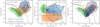 |
Fig. 1. Comparison between the classical BPT and the new proposed diagnostic diagram for integrated properties. Left panel: Classical BPT diagram (Baldwin et al. 1981), showing the distribution of [O III]/Hβ line ratio as a function of [N II]/Hα ratio. It includes four sub-samples of objects whose ionization has been classified according to this diagram together together with EW(Hα), following Sánchez et al. (2021): (i) star-forming galaxies (SF, green), (ii) retired galaxies (RG, orange), (iii) optically selected AGNs (O-AGNs, blue), and (iv) X-ray selected AGNs (X-AGNs, black stars). Solid symbols correspond to data extracted from the eCALIFA sample, with the X-AGNs being extracted from Osorio-Clavijo et al. (2023). The shaded regions correspond to data extracted from the MaNGA sample (SF, RG, and O-AGNs) and from Agostino & Salim (2019) (X-AGNs), showing the area encircling 90% of the objects in each case. The region at which the ionization was measured is indicated in the legend: central aperture (cen) or at the effective radius (Re). Solid and dot-dashed lines correspond to the classical demarcations lines proposed by Kauffmann et al. (2003) and Kewley et al. (2001) to distinguish between the different ionizing sources. Middle panel: New proposed diagnostic diagram (WHaD) showing the distribution of the EW(Hα) (or WHα) as a function of the Hα velocity dispersion for the same sub-samples of objects included in the previous panel, using the same nomenclature. It is clearly appreciated that the different ionizing sources are well separated in this new diagram. Dashed lines correspond to the proposed demarcation lines to separate between different dominant ionizing sources, with the corresponding sources indicated. Right-panel: Distribution in the BPT diagram shown in the first panel of the eCALIFA (solid symbols) and MaNGA (shadded regions) galaxies classified according to the location of their ionization in the WHaD diagram, measured at the same two locations indicated adopted for the values shown in the first panel. The location of the X-ray selected AGNs has been included for completness. |
This approach is often far too simplistic and overly biased by the overwhelming number of explorations using single aperture spectroscopic surveys (e.g., SDSS or GAMA; York et al. 2000; Driver et al. 2009). First, the so-called intermediate regime could be populated by ionization purely related to a recent SF event, particularly in the presence of super-nova remnants (e.g., Cid Fernandes et al. 2021), or by ionization due to low-metallicity AGNs. This is indeed confirmed when exploring the location of X-ray selected AGNs in this diagram (X-AGNs, e.g., Agostino & Salim 2019; Osorio-Clavijo et al. 2023; Agostino et al. 2023) Thus, the concept of intermediate or mixed region is often misleading – at least in general, despite the fact that this regime may indeed be populated by a mix of SF processes and harder ionization sources (Davies et al. 2016; Lacerda et al. 2018).
Finally, it is well known that other ionizing sources can mimic the line ratios usually associated only with AGNs when using this classification scheme. For instance, shocks present a wide variety of line ratios depending on the properties of the ionized gas, the strength of the magnetic field, and the velocity of the shock. High-velocity ones, namely, those associated with galaxy-scale outflows (e.g., López-Cobá et al. 2020), have line ratios similar to those observed in strong AGNs (e.g., Veilleux et al. 2001). On the contrary, low-velocity ones, which are observed, for instance, in certain elliptical galaxies, present much lower line ratios (e.g., Dopita et al. 1996). Another key ionizing source in these kinds of galaxies and in non-SF retired galaxies in general (RG; Stasińska et al. 2008), or retired regions within galaxies (e.g., Singh et al. 2013; Belfiore et al. 2017; Lacerda et al. 2018), is the one produced by hot evolved and post-AGB stars (Binette et al. 1994). The ionization by this stars produces weaker emission lines than those due to SF or AGNs (and shocks in many cases). However their line ratios cover a wide range of values, being as low as the values usually associated with SF or as high as those classically assigned to AGNs (Sánchez 2020). Hereafter, we refer to this ionization as RG.
The distribution in the O3–N2 BPT diagram of both shocks and post-AGB ionization is very similar (e.g., Sánchez et al. 2021). They cover the regime from the bottom-end of the SF distribution expanding towards larger values of both line ratios until reaching the same regime covered strong AGNs. They can also cover the same area known as low-ionization nuclear emission region (LINER; Heckman 1987), which is nowadays not considered to be produced by low-luminosity AGNs in all the cases. Therefore, the line ratios adopted by the traditional BPT are not sufficient to separate between certain ionizing sources. To circumvent this problem, different strategies have been proposed. For instance, Cid Fernandes et al. (2010) introduced the WHaN diagram, using the equivalent-width of Hα, EW(Hα), or WHα, a tracer of the relative intensity of the emission lines with respect to the underlying continuum, and the N2 ratio, as a tracer of the hardness of the ionization. In this diagram, SF and AGNs are consider to have large values of EW(Hα), with the former having lower values of N2 that the later. Regions ionized by hot evolved stars present low values of EW(Hα) (< 3 Å), irrespective of the N2 value. Based on a similar reasoning, Sánchez et al. (2014) proposed to combine the O3–N2 BPT diagram with the EW(Hα) to clean the SF regime from the contamination by low-N2 RG sources. Later Sánchez et al. (2018) generalized this idea, introducing the BPT+WHa diagram, in which the ionization is classified using both the BPT diagram and the EW(Hα) for all the considered ionizing sources.
The use of EW(Hα) helps to distiguish between RG and both SF and AGNs where they overlap in the BPT diagram. However, it does not completely solve the problem of identifying the dominant ionizing source. For instance, in the case of shocks, both the location in the BPT diagram and the value of the EW(Hα) could be similar to that observed for AGNs (and SF in some cases). One possible solution is to explore the shape of the ionized structure, what it is only possible when spatial resolved spectroscopic data is available (e.g., Jarvis 1990; López-Cobá et al. 2017, 2019). An alternative strategy is to introduce the asymmetries in the emission lines and the velocity dispersion as an additional parameter to distiguish between different ionizing sources or a combination of those kinematics parameters with the BPT, the location within the galaxy and/or the galactocentric distance (D’Agostino et al. 2019; López-Cobá et al. 2020; Johnston et al. 2023).
Methods that include the velocity information are indeed physical motivated: (1) SF happens in disks and it requires low velocity dispersions to be triggered and (2) RG is associated with hot-evolves stars, which are generally found in bulges or thick disks, namely, they are associated with regions of larger velocity dispersions than disks; (3) AGN ionization happens in the so-called narrow-line regions2, which (despite the name) present much larger velocity dispersions than galaxy disks; and, finally, (4) shock ionization, which (by its very nature) is associated with high-velocity dispersion clouds, due to the result of the compression and non uniform propagation of the galactic winds (shocks also produce multi-component and asymmetric emission lines). A recent exploration by Law et al. (2022) demonstrates that SF ionization is statistically associated with low velocity dispersion emission lines (σvel ∼ 25 km s−1), while harder ionizations are associated with a wide range of velocity dispersions, generally larger than > 50−60 km s−1. Indeed, the average distribution of the ionized gas velocity dispersions across the BPT diagram follows a similar, but opposite, pattern to that described by the EW(Hα) (e.g., Lacerda et al. 2018; Sánchez et al. 2021, 2022).
Often the methods described above are insufficient. Determining the nature of the ionization requires the use of additional information, such as the shape of the ionized structures, fraction of young stellar populations, location with in the galaxy, and the galactocentric distance (e.g., D’Agostino et al. 2019; López-Cobá et al. 2020; Espinosa-Ponce et al. 2020; Sánchez et al. 2021; Johnston 2022). The more additional parameters are used, the more complicated it is to observe all of them simultaneously with the required signal-to-noise ratio (S/N) needed to provide reliable classifications. Diagnostic diagrams based on line ratios require the simultaneous determination of the flux of four emission lines, not all of them being of the same relative intensity (or S/N). For instance, in the case of the O3–N2 diagram, it is often the case that Hβ is the limiting parameter. Ionizing sources that generate intrinsically weak emission lines, such as post-AGB and hot evolved stars, produce Hα fluxes that are barely detectable with the current spectroscopic galaxy surveys in many cases. In those cases, the Hβ is about three times weaker and remains frequently undetected. A similar situation may happens in the presence of strong dust attenuation, as in the case of ultraluminous infrared galaxies, despite the intrinsic luminosity of the ionized gas emission. As expected the situation becomes more complicated when more parameters are introduced. Therefore, the search for a more accurate classification is often hampered by the precision required for the involved parameters to be estimated.
One additional problem seen for most classical diagnostic diagrams like the BPT is the use of lines appearing in several different spectral regions. Due to technical limitations or the design of the spectrograph, the lines cannot be observed simultaneously in a single setup (e.g., MEGARA; Gil de Paz et al. 2018) or even with a single spectrograph (MUSE; Bacon et al. 2010, and the need for BlueMUSE). These problems disappear when the available diagnostics are based on a single line.
Motivated by the limitations of the currently adopted procedures to classify the ionizing source and based on the most recent explorations that consider both the EW(Hα) and σvel as key parameters in this regard, we present a single emission line diagnostic diagram that uses only those two parameters (named WHaD, hereafter). We demonstrate that this diagram determines the nature of the ionizing source as well as the combination of the BPT diagram with the EW(Hα), with the advantage of using just one single line and two parameters. We illustrate its use by comparing the spatial resolved classification of the ionizing source provided by the WHaD diagram with that provided by the BPT+WHa for a few archetypal galaxies, providing access to a similar comparison for a large galaxy sample.
The distribution of this article is as follows: the different datasets employed in this study are presented in Sect. 2, with both the analysis and results included in Sect. 3. Finally, the main conclusions are summarized in Sect. 4.
2. Data
We made use of the data products provided by the pyPipe3D pipeline (Lacerda et al. 2022) for the integral field spectroscopy (IFS) data provided by the extended Calar Alto Legacy Integral Field Area (eCALIFA) survey (Sánchez et al. 2012, 2023b), and the final distribution of the Mapping Nearby Galaxies at Apache Point Observatory (MaNGA) survey (Bundy et al. 2015). Both surveys have been extensively described in the literature, particularly in works describing their most recent and final data releases (Sánchez et al. 2016a, 2023a; Abdurro’uf et al. 2022), with a comparison between them included in a recent review on the topic of IFS galaxy surveys (Sánchez 2020).
To avoid repetitions, we do not include a throughfull description of those surveys here. For the purposes of the current exploration, we should highlight that: (i) both surveys observe a representative sample of galaxies in the nearby universe (zCALIFA ∼ 0.015, zMaNGA ∼ 0.045), covering a wide range of galaxy types and stellar masses, being complete above M⋆ ∼ 109 M⊙, once applied the proper volume correction; (ii) the sample of galaxies is about ten times larger in the case of MaNGA (∼9000 objects with good quality data) with respect to the sample covered by eCALIFA (895 objects), but the field of view of the IFS data (74″ vs. 19−32″), the spatial coverage (2.5 Re vs. 1.5−2.5 Re), sampling and physical resolution (∼0.3 kpc vs. ∼2 kpc) is better (or larger) in the case of eCALIFA (in average); (iii) the spectral range (resolution) of the MaNGA data is about two times larger (better) than that of eCALIFA, R ∼ 2000 vs. ∼850, respectively. Nevertheless, in both cases, this is good enough for the purposes of this study; finally (iv) both surveys cover the emission lines of interest for the current exploration (Hβ, [O III], Hα, and [N II]), with a high enough S/N to measure the flux intensities, velocity dispersion, and equivalent widths for the vast majority of the observed objects.
The automatic pipeline pyPipe3D performs a spectral decomposition of the stellar continuum and the ionized gas emission lines based on the stellar synthesis tecnique, assuming a particular template of single stellar populations (Sánchez et al. 2016b; Lacerda et al. 2022). This pipeline has been used extensively to study IFS data from different datasets, including CALIFA (e.g., Cano-Díaz et al. 2016; Espinosa-Ponce et al. 2020), MaNGA (e.g., Ibarra-Medel et al. 2016; Barrera-Ballesteros et al. 2018; Sánchez et al. 2019a; Bluck et al. 2020; Sánchez-Menguiano et al. 2019), SAMI (e.g., Sánchez et al. 2019b), and AMUSING++ (Sánchez-Menguiano et al. 2018; López-Cobá et al. 2020). In addition, it has been tested using mock datasets based on hydrodynamical simulations (Guidi et al. 2018; Ibarra-Medel et al. 2019; Sarmiento et al. 2023). To avoid unnecessary repetition we do not include a description of the pyPipe3D either.
For the purpose, of the current exploration it is relevant to know that for each analyzed datacube, pyPipe3D provides the spatial distribution of a set of physical and observational parameters derived for both the stellar population and the ionized gas. In this study, we made use of the spatial distributions of: (i) the flux of the emission lines involved in the O3–N2 BPT diagram, (ii) the Hα velocity dispersion (corrected by instrumental resolution), and (iii) the EW(Hα); all of these were recovered based on the non-parametric moment analysis peformed by this pipeline on the pure gas datacubes (i.e., the datacube once the best model spectra for the stellar component has been subtracted). All of these dataproducts are publicly available distributed by Sánchez et al. (2022, 2023a,b), as part of the corresponding eCALIFA and MaNGA data releases. The average value of each of these parameters at both the effective radius (Re) and in the central region of each galaxy (1.5″ diameter and 2.5″ diameter for eCALIFA and MaNGA, respectively) was also released.
In addition, we made use of the results by Osorio-Clavijo et al. (2023), which have recently explored the X-ray properties of a sub-sample of the CALIFA galaxies, recovering ∼40 bona-fide AGNs. Finally, we used the O3 and N2 values of the sample of X-ray selected AGNs presented in Agostino & Salim (2019) for comparison purposes.
3. Analysis and results
3.1. Classifying the ionization using the classical BPT diagram
As indicated in the introduction, the procedure most frequently used to classify the ionization is the location of the O3 and N2 line ratios in the BPT diagram that has been combined, in some cases, with an additional parameter, for instance the EW(Hα). Figure 1 (left-panel) shows the distribution (in this diagram) of the different data sets described in the previous section, classified following the prescriptions outlined in Sánchez et al. (2021), hereafter noted as the BPT+WHα scheme: (1) RG: galaxies with EW(Hα) at Re below 3 Å, irrespectively of the location of the line ratios in the BPT diagram, not belonging to any of the other groups; (2) SF: galaxies with EW(Hα) > 6 Å and line ratios below the Kewley et al. (2001) demarcation line at Re, and not belonging to any of the other groups; (3) O-AGNs: galaxies with a EW(Hα) > 6 Å and line ratios above the Kewley et al. (2001) in the central aperture. We note that O-AGNs, are frequently distinguished on the basis of strong and weak AGNs, adopting EW(Hα) ∼ 10 Å as the boundary between both categories. For AGNs, we selected the central aperture due to the dilution effect introduced by the ionized gas from the host galaxy (e.g., Sánchez et al. 2018; Osorio-Clavijo et al. 2023; Albán & Wylezalek 2023). Finally, we included the X-AGNs extracted from Osorio-Clavijo et al. (2023) and Agostino & Salim (2019), Agostino et al. (2023). We note that most objects were well classified using this scheme, with just a few objects lacking a well-defined dominant ionizing source.
By construction, the SF galaxies are located where it is expected. They follow a clear arc-shaped distribution not only below the adopted demarcation line (Kewley et al. 2001), but in most of the cases below the more restrictive Kauffmann et al. (2003) one (∼92% of the objects). A similar behavior is found for the O-AGNs, which (by construction) are located above the Kewley et al. (2001) curve. Thus, SF can be distinguished from O-AGNs using just the BPT diagram and the classical demarcation lines. However, the situation is not that simple when RGs are included. It is clear that galaxies (and regions within them) with low EW(Hα) are distributed in the right-branch of the BPT diagram, covering a wide range of values. Some 17% of them are below the Kauffmann et al. (2003) curve, ∼54% in the intermediate region between that line and the Kewley et al. (2001) one, and ∼28% above that line. Thus, without introducing an additional parameter, in this case the EW(Hα), it is not possible to distinguish between this ionizing source and SF or O-AGNs.
We should note that the current selection of O-AGNs does not guarantee that all AGNs are selected. It is well known that in many instances, radio galaxies do not present signatures of optical AGNs regarding their line ratios and/or flux intensities (e.g., Comerford et al. 2020, and references therein). Other bona fide AGNs, such as those detected in X-rays, present emission lines in the optical with ratios that are not above the demarcation lines adopted to select O-AGNs in many cases. We include in Fig. 1 (left panel), the distribution of the 424 X-ray selected AGNs by Agostino & Salim (2019) and Agostino et al. (2023) (X-AGNs, hereafter), with the emission lines obtained from the SDSS spectroscopic data. It is clear that they are not restricted to the same regime usually adopted to select O-AGNs, covering a range of values more similar to the one observed for RG. Indeed, in the case of this particular sample of X-AGNs, only 34% of them would be classifed as O-AGNs, 28% as RGs and 20% as SF galaxies, using the BPT-WHα classification scheme (Sánchez et al. 2021). This is usually interpreted as a dilution effect by the contamination of other ionizing sources (e.g., circumnuclear or host-galaxy star-formation) or any obscuration of the optical emission. However, a similar behavior is observed in the distribution of the line ratios extracted from the central aperture (< 1 kpc) of the X-AGNs selected from the CALIFA sample itself studied by Osorio-Clavijo et al. (2023). In this case the fraction of objects classified as O-AGNs is even lower (17%), using the BPT-WHα scheme. Furthermore, Agostino et al. (2021) demonstrated that once subtracted the SF contribution to the integrated SDSS spectra of a sample of Seyfert galaxies a large number of them are still found below the Kauffmann et al. (2003) demarcation line. In summary, neither the BPT along nor its use combined with the EW(Hα) guarantee a clean separation of AGNs from other ionizing sources.
3.2. BPT-classified ionizing sources across the EW(Hα)–σHα (WHaD) diagram
We go on to explore the ability to classify the ionizing source using just the EW(Hα), which has been proved to be crucial to distinguish between RG and other ionizing sources as well as the velocity dispersion (σvel, following D’Agostino et al. 2019; López-Cobá et al. 2020; Law et al. 2022; Johnston 2022). Figure 1 (central panel) shows the distribution of the EW(Hα) as a function of σHα (hereafter the WHaD diagram) for the same dataset included in the BPT diagram (left-side diagram). It is clear that that three categories of ionizing sources selected using the BPT+WHα are located in three distinguishable regions. SF galaxies are all restricted to a narrow range of low velocity dispersions and high EW(Hα). Indeed, as already noticed by Law et al. (2022), there is a very low number of SF galaxies with a velocity dispersion above > 50 km s−1 (∼2%), with most of them located in the regime of ∼25 km s−1. On the other hand, RG ocupy the regime of low EW(Hα) by construction. In addition, they cover a wider range of velocity dispersions, from ∼30 km s−1 to ∼300 km s−1, with an average value ∼90 km s−1 (slightly lower for eCALIFA than for MaNGA). Finally, the O-AGNs are limited to a regime of high EW(Hα) by construction, covering an even wider σHαrange, with larger values for MaNGA than for eCALIFA. Regarding the X-AGNsm we do not have the required information to replicate the distribution shown in the BPT diagram for the Agostino & Salim (2019) dataset; however, the sample studied by Osorio-Clavijo et al. (2023) distributed across the entire diagram, with a preference to larger velocity dispersions than the SF sample.
We quantified the ability to segregate the different ionizing sources using the WHaD diagram in comparison with the BPT one by performing a 2D Kolmogorov–Smirnov (KS) test (using the NDTEST python package3). Table 1 lists the values of the KS statistics obtained by comparing the distributions of the different ionizing subsamples selected based on the BPT+WHα criteria applied to the MaNGA dataset (SF, RG, and O-AGNs) in addition to the Agostino & Salim (2019) sample (X-AGNs) across the O3–N2 BPT and the WHaD diagrams. We adopted these subsamples as they offer the largest number of objects (i.e., better statistical coverage of the explored parameters). The result of this test indicates that the new diagram segregates the different subgroups in a more efficient way.
Results of the 2D Kolmogorov–Smirnov test.
Based on the described distributions and the results of the KS-test, we defined five regimes in the WHaD diagram. First, using the same criteria cited by Cid Fernandes et al. (2010) when introducing the WHaN diagram (also adopted in the BPT+WHα scheme), we classified as RG those sources with an EW(Hα) < 3 Å. Then we classified as SF those sources with a EW(Hα) > 6 Å (following Sánchez et al. 2014) and σHα < 57 km s−1, a region that comprises 98% (90%) of the eCALIFA (MANGA) previously selected SF galaxies. In addition, we define as O-AGNs those sources with a EW(Hα) > 3 Å and a σHα > 57 km s−1, distinguishing between weak-AGNs (wAGN) and strong-AGNs based on the EW(Hα), using 10 Å as a boundary between both regimes. Based on these criteria 86% (95%) of the O-AGNs selected using the BPT+WHα scheme would remain as O-AGNs, and 14% (1%) would be reassigned as SF in the case of the eCALIFA (MaNGA) sample. We note that the boundary in the velocity dispersion was empirically selected to maximize (minimize) the agreement (disagreement) between the classifications provided by the classical BPT diagram and the new proposed WHaD diagram for the optically selected SF and O-AGNs.
If we consider the fact that the BPT–WHα scheme does actually reproduce the real distribution of ionizing sources, the new classification based on the WHaD diagram would be 100% reliable for the RG (as it is essentially the same scheme), between a 90–98% reliable for SF galaxies, and just a 86–95% reliable for O-AGNs. However, we should keep in mind that the initial scheme is based on some pre-conceptions, like the fact that AGNs should present strong emission lines produced by a hard ionization (i.e., high values of both O3 and N2). As indicated before this is not always the case. Figure 1, left and central panels, shows that bona-fide X-AGNs may present a wide range of O3–N2 line ratios and an equaly wide range of EW(Hα) values. Regarding X-AGNs, we already established that only 17–34% of those studied by Osorio-Clavijo et al. (2023) and Agostino & Salim (2019) are classified as O-AGNs using the BPT+WHα scheme. This fraction increases to a 50–53% when using the newly introduced WHaD classification procedure. This is particularly relevant, as X-AGNs are the only sources for which the ionization source is fully determined. Based on these results, we should not consider that a priori the BPT-WHα offers a better classification scheme than the currently proposed one.
3.3. Classifying the ionization using the WHaD diagram
Based on this exploration, we re-classified the eCALIFA, MaNGA galaxies, and the X-AGN samples studied in the previous sections using the new WHaD diagram and the boundaries proposed before. Figure 1, right-panel, shows the distribution along the O3–N2 BPT diagram based on this new classification, using the same nomenclature as the one adopted in the left and central panels. As a first result, we highlight that the distribution for RGs is the same. Regarding the SF galaxies, besides the increase in the number of galaxies (plus 8%), the distributions are very similar. Only ∼1% of the newly classified SF galaxies would be classified as AGNs using the BPT+WHα scheme. The main difference is found for the O-AGNs, that now are not restricted to the upper-end of the right-branch in the BPT diagram. Indeed, they follow a distribution more similar to that of the RG or the X-AGNs in this diagram. About 27% (50%) of the eCALIFA (MaNGA) galaxies classified as O-AGNs with the new WHaD scheme would be SF based on the BPT+WHα method. Although this could be due to a missclassification introduced by the new procedure, we consider more probable that we have disclosed a larger population of AGNs thanks to the new method.
As a final remark, we stress that the results for both datasets, eCALIFA and MaNGA, are remarkable similar despite of the reported differences between the two datasets, outlined in Sect. 2. The major differences are found in the fraction of previously selected O-AGNs (SF) that are not classified as SF (O-AGNs), where both samples disagree by ∼20%. In this regard, we remind that both samples have different selection functions and so far we have not applied any correction for the selection function. Thus, the reported differences could be just due to the different sample selections.
3.4. Spatial distribution of the ionizing sources using the WHaD diagram
In the sections above, we describe how the dominant ionizing source was determined for different galaxies (and apertures within them), using a rather classical, well-stablished approach (Sect. 3.1) in comparison with the new scheme proposed in this study (Sects. 3.2–3.3). As already indicated in the introduction, and discussed in several previous studies (e.g., Sánchez 2020; Sánchez et al. 2021, and references therein), the ionization is a process that happens at scales smaller than the ingrated galaxy scale discussed in the previous sections. As in the case of the integrated or aperture-limited spectra (e.g., Kauffmann et al. 2003), diagnostic diagrams and/or a combination of them with additional parameters has served as a well established procedure to identify the different ionizing sources that may be present in a galaxy when using spatial resolved spectroscopy data (e.g., Law et al. 2022; Johnston 2022; Sánchez et al. 2023a, citing just a few). To demonstrate that the WHaD diagram provides with a spatial resolved classification of the ionizing source as good (or even better) than the one provided by the BPT+WHa scheme, we have applied both methods to the spatial resolved dataproducts derived using pyPipe3D for the full IFS dataset provided by the last eCALIFA data relase (Sánchez et al. 2023a,b), already described in Sect. 2. We distribute the outcome of this analysis through the web4, describing here in detail the results derived for four cherry-peaked galaxies that illustrate the general behavior.
Figure 2 shows the comparison between the spatial resolved distribution of the ionizing sources identified based on the BPT+WHα scheme and the WHaD diagram for NGC 5947. This is a low-inclination early spiral, with a morphology (SBbc) and stellar mass (∼1010.5 M⊙) that are very similar to that of the Milky-Way (indeed, it hosts a solar-neighborhood analog region too; Mejía-Narváez et al. 2022). Figure 2 (top-left panel) shows an optical three-color image extracted from the datacube that traces the light distribution from the stellar continuum. Contours trace the distribution the combined flux itensities of Hα and [N II]. As expected, the regions with stronger ionized-gas emission trace the location of the spiral arms, although there is detectable ionized gas across most of the optical extension of the galaxy. The distribution across the [O III] versus [N II] diagnostic diagram for the individual spaxels is included in the top-middle panel, color-coded according to the BPT+WHa classification scheme (Sect. 3.1), with the spatial distribution of the different ionizing sources shown in the top-right panel. In this particular implementation of the classification scheme, we considered that the ionizing source cannot be correctly identified if the S/N of Hα is lower than 3, and below 1 for the remaining emission lines involved in this diagram. We note that for the identification of retired regions, this criteria could be relaxed, adopting just a cut in EW(Hα). As expected, due to the nature of this galaxy, most of the optical extension is dominated by ionization related to recent SF. Only a small annular circumnuclear region of ∼5″ presents an ionization classified as retired (or unknown). Finally, based on this scheme the ionization in the central region (< 3″) is classified as SF.
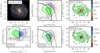 |
Fig. 2. Comparison between the classical BPT and the new proposed diagnostic diagram for resolved properties. Top-left panel: RGB-image created using the r-, g-, and r-band images synthetized from the eCALIFA datacube of NGC 5947, together with a set of contours showing the Hα+[N II] flux intensities, with the 1st contour corresponding to the mean value minus one standard deviation, and each sucesive contour followig a multiplicative scale of five times that value. The red-circle indicates the central aperture adopted along this article (e.g., Fig. 1). Top-middle panel: Classical diagnostic diagram showing the distribution of [O III]/Hβ line ratio as a function of the [N II]/Hα ratio for each individual spaxel of the same cube shown in the top-left panel, color coded by nature of the ionization according to the classification based on locaton in this diagram together with the EW(Hα), thus, the same selection criteria adopted in top-left panel of Fig. 1: SF in green, RG in orange and AGN-like ionization in blue. Top-right panel: Spatial distribution of the ionized gas for those spaxels with Hα above the mean minus one standard deviation value, color coded by the classication shown in the middle panel (i.e., BPT+WHα). Those spaxels with Hα flux with a S/N below 3 or any of the remaining emission lines involved in the BPT diagram below 1 are marked as unknown (dark-red color). Contours are the same already shown in the top-left panel. Bottom-left panel: Distribution along the WHaD diagram, EW(Hα) versus σHα, for the individual spaxels of the same datacube shown in the previous panels, color coded according to the classification of the ionizing source based on the location within this diagram. Bottom-middle panel: Diagnostic diagram similar to the one already shown in top-middle panel, with the individual spaxels color coded following the new classification based on the WHaD diagram (bottom-left panel). Bottom-right panel: Spatial distribution of the ionized gas similar to that shown in the top-right panel, this time color-coded with the classification obtained using the WHaD diagram shown in the bottom-left. The similarities and differences between the two classiciation schemes are evident when comparing top- and bottom-right panels. |
The distribution of spaxels along the WHaD and BPT diagrams for NGC 5947 are included in bottom-left and bottom-central panels of Fig. 2, color-coded according to the new classification scheme (Sect. 3.3), with the spatial distribution of the new classified ionizing sources shown in bottom-right panel. Despite of the fact that the distribution across the BPT diagram looks very different, the spatial distribution of the different ionizing sources is rather similar. Most of the spaxel are classified as SF, covering a similar region as the one covered by the previous classification, roughly corresponding to the disk of the galaxy. The annular region around the center is equally classified as retired (or unknown). However, contrary to the previous classification, the ionization in the central region is classified as wAGN or sAGN. Based on the results discussed in previous sections we cannot conclude that this is a miss-classification, as up to ∼20% of bona-fide AGNs (e.g., X-AGNs) could present line ratios compatible with SF, even when the spectroscopic information is restricted to the central apertures (e.g., Agostino & Salim 2019; Osorio-Clavijo et al. 2023). On the other hand, we cannot neither exclude the possibility that this is a misclassification that may have been introduced by the new method. So far, the presence of an AGN has not been confirmed in NGC 5947 using non-optical observations.
Figure 3 presents similar plots for NGC 2906. This is a late-type, almost face-on, spiral galaxy slightly less massive than NGC 5947 (M⋆ ∼ 1010 M⊙). As in the previous case, the ionization is classified as SF for most of the regions, in particular, for those in the galaxy disk. However, contrary to the previous galaxy, all the ionization in the central regions (< 10″) is classified as retired (or unknown). The two classification schemes (BPT+WHa and WHaD) provide very similar results. Thus, the spatial distributions of the ionizing sources included in top- and bottom-left panels of Fig. 3 are almost undistiguisable. However, when looking in detail, the WHaD scheme classifies a circular region region ∼12″ north and ∼5″ east from the center of the galaxy as as a wAGN or sAGN. On the contrary, based on the BPT+WHa method, the ionization at this location would be classified as SF. Like in the previous case we could consider that this is misclassification of the new method, as obviously an off-center AGN is unlikely. However, it is known that a supernova exploded in this galaxy at this exact location before the observing run (SN 2005ip, Lee et al. 2005), and where a supernova remnant has been identified (Martínez-Rodríguez, in prep.). We must recall that AGN ionization cannot be distinguished from other sources of ionization such as shocks or SNRs based only in the exploration of the BPT diagram, and additional parameters have to be introduced (e.g., López-Cobá et al. 2020; Cid Fernandes et al. 2021, and in the introduction). However, the WHaD diagram seems to pinpoint SNRs that are well below the classical demarcation lines adopted to separate SF regions from other sources of ionization.
Motivated by the previous result, we explore how the classifications that are based on the two methods compare in the presence of evident shock ionization. Figure 4 shows the same plots already included in Figs. 2 and 3 for the edge-on spiral galaxy NGC 6286. This is a luminous infrarred galaxy (Howell et al. 2010) that presents a well studied galactic outflow (e.g., López-Cobá et al. 2019, and references therein). This outflow is easily identified in the Hα+[N II] flux intensity contours included in the top-left panel of Fig. 4, having the archetypical biconical shape. The origin of this galactic outflow is under discussion. Based on pure optical spectroscopic data and following the criteria defined by Sharp & Bland-Hawthorn (2010), López-Cobá et al. (2019) determined that this outflows is most probably driven by a strong nuclear SF process. However, it known that this object host an obscured AGN (Ricci et al. 2016), that has been uncovered using X-ray observations. Irrespectively of the physical origin of the galactic wind that generated the outflow, the gas along its biconical structure is clearly ionized by shocks. This is appreciated in top-central and top-right panels of Fig. 4: using the BPT+WHa criteria the ionized gas at the location of the outflows is classified as wAGN/sAGN. We note again that this is expected for a shock-ionized gas. In addition, the gas along the edge-on disk is mostly ionized by a SF process. When applying the new classification scheme (bottom panels), we find a very similar result, with subtle differences (for instance, the width of the regime classified as SF along the edge-on disk is slightly narrower when using the new scheme). We performed a visual inspection of all the galaxies with detected outflows within the CALIFA sample (López-Cobá et al. 2019), finding similar consistent results. In summary, using the WHaD diagram it is feasible to identify shock-ionized galacitc outflows as well as using the BPT+WHa scheme.
Finally, Fig. 5 is organized in a similar way to Figs. 2–4, but for an archetypical retired galaxy, NGC 3610. This is an intermediate-mass (M⋆ ∼ 1010.3 M⊙) elliptical galaxy, with a weak and diffuse ionized gas emission distributed across most of the FoV of the IFU data (top-left panel of Fig. 5). It presents a weak and soft X-ray emission that is not compatible with the presence of an AGN (Fabbiano & Schweizer 1995). Despite of the nature of this object (a true elliptical galaxy or a an early-spiral with a very low dist-to-bulge ratio), its ionized gas is clearly classified as retired using the BPT+WHa (top-central and top-right panels of Fig. 5). We note that a substantial fraction of the spaxels with detected ionized gas would be classified as unknown if a cut in the S/N of all the lines involved in the BPT diagram is considered. Using just the EW(Hα) they would be classified as retired, being most probably ionized by hot evolved low mass stars in the post-AGB phases. By construction, the WHaD diagram performs a similar classification, with the difference being that most of the regions which ionizing source is labeled as unknown when using the full dataset required to explore the BPT diagram are known directly classified as retired.
In summary, we have illustrated how the use of the WHaD classification scheme, based on one single emission line, provides a reliable classification of ionizing source for the spatial resolved ionized gas in galaxies. This classification is compatible, in general, with the one provided by the BPT+WHa scheme. The reported differences may reflect possible cases of misclassification (e.g., central AGN in NGC 5947) or the uncover of previously undetected or missed ionizing sources (e.g., central AGN in NGC 5947 again and the SNR in NGC 2906).
4. Conclusions
This work is motivated by the need to discuss the issues in identifying the ionizing source in galaxies based on the most commonly used method. This method uses the O3 versus N2 BPT diagram, identifying regions in which different ionizing sources are dominant or more frequently observed. The method present intrinsic problems, due to (i) the S/N requirements and the wide range of relative fluxes between the involved emission lines, and (ii) the confusion among regimes in which different ionizing sources could be reproducing the observed line ratios. While the later problem has been addressed in the literature by the inclussion of additional parameters, such as EW(Hα) and/or σvel, to overcome these problems, although the former one cannot be addressed in a straightforward manner.
We have proposed an new method that explores the location of different ionizing sources in a new diagram (WHaD), which compares EW(Hα) and σvel. This diagram has the virtue of using just one single emission line, typically the strongest one in the optical range for all ionizing sources. We used IFU data from eCALIFA and MaNGA in combination with literature data to explore the location of different ionizing sources classified using the standard procedure (BPT+WHa method) and bona-fide X-ray selected AGNs. Based on that exploration, we defined different areas in which the ionizing source could be classified as: (i) SF, ionization due to young-massive OB stars, related to recent star-formation activity; (ii) sAGNs/wAGNs, ionization due to strong (weak) AGNs, and other sources of ionizations like high velocity shocks; and (iii) RG, ionization due to hot old low-mass evolved stars (post-AGBs), associated with retired galaxies and regions within galaxies (in which there is no star-formation).
We applied the new classification to (i) the same dataset adopted to define the method and (ii) the full dataset of spatial resolved spectroscopic data provided by the eCALIFA survey, comparing the results provided by the two methods (BPT+WHa vs. WHaD). We found that:
-
Both methods provide exactly the same classification for retired regions and galaxies, when only EW(Hα) is considered. If the full set of emission lines required to explore the BPT diagram is used the new method recovers a larger number of galaxies/regions that cannot be classified using the BPT+WHa method.
-
90% (i.e., 86–95%) of the galaxies classified as SF (O-AGNs) using the BPT+WHa method would be classified as the same using the WHaD diagram.
-
Around 99% (50–73%) of the galaxies classified as SF (O-AGNs) using the WHaD diagram were equally classified using the BPT+WHa method.
-
Around 50% of the X-AGNs have been classified as O-AGNs using the WHaD method, a significantly larger fraction than the number than the one recovered using the more traditional BPT+WHa diagram (17–34%).
-
The spatially resolved classification provided by the WHaD is similar to the one provided by the BPT+WHa one for star-forming, retired, and high-speed shock-ionized regions. However, it increases the number of AGN candidates and AGN-like ionizing sources, which additionally have a more realistic distribution in the BPT diagram than the one shown by O-AGNs.
In summary, we consider that the proposed method is an useful tool when all the set of emission lines required for other diagnistic diagrams are not accessible due to the wavelength range covered by the observations (e.g., in Fabry-Perot observations in many cases) or some of them lack sufficient S/N for a proper exploration (e.g., in the case of Hβ for dusty galaxies or regions within galaxies). The method has been proved for low-z (z ∼ 0.01) integrated and spatially resolved data. Any attempt to apply it at higher redshifts would require a re-evaluation of the method and the proposed boundaries, which is beyond the scope of the current exploration.
The list of references using this scheme is too large to cite them here.
For type-II AGNs, as type-I are the more easy ones to be identified by their distinguish feature of having broad Balmer lines.
Acknowledgments
We thanks the anonymous referee for the comments that have improved this manuscript. SFS thanks support from Conacyt FC G-543 grant, S.F.S. thanks the PAPIIT-DGAPA AG100622 project. J.K.B.B. and S.F.S. acknowledge support from the CONACYT grant CF19-39578. J.S.A. acknowledges financial support from the Spanish Ministry of Science and Innovation (MICINN), project PID2019-107408GB-C43 (ESTALLIDOS). Integral Field Area (CALIFA) survey (http://califa.caha.es/), observed at the Calar Alto Obsevatory. Based on observations collected at the Centro Astronómico Hispano Alemán (CAHA) at Calar Alto, operated jointly by the Max-Planck-Institut für Astronomie and the Instituto de Astrofísica de Andalucía (CSIC). This project makes use of the MaNGA-Pipe3D dataproducts. We thank the IA-UNAM MaNGA team for creating this catalogue, and the Conacyt Project CB-285080 for supporting them. This research made use of Astropy (http://www.astropy.org), a community-developed core Python package for Astronomy (Astropy Collaboration 2013, 2018). Funding for the Sloan Digital Sky Survey IV has been provided by the Alfred P. Sloan Foundation, the US Department of Energy Office of Science, and the Participating Institutions. SDSS-IV acknowledges support and resources from the Center for High Performance Computing at the University of Utah. The SDSS website is www.sdss.org. SDSS-IV is managed by the Astrophysical Research Consortium for the Participating Institutions of the SDSS Collaboration including the Brazilian Participation Group, the Carnegie Institution for Science, Carnegie Mellon University, Center for Astrophysics, Harvard & Smithsonian, the Chilean Participation Group, the French Participation Group, Instituto de Astrofísica de Canarias, The Johns Hopkins University, Kavli Institute for the Physics and Mathematics of the Universe (IPMU)/University of Tokyo, the Korean Participation Group, Lawrence Berkeley National Laboratory, Leibniz Institut für Astrophysik Potsdam (AIP), Max-Planck-Institut für Astronomie (MPIA Heidelberg), Max-Planck-Institut für Astrophysik (MPA Garching), Max-Planck-Institut für Extraterrestrische Physik (MPE), National Astronomical Observatories of China, New Mexico State University, New York University, University of Notre Dame, Observatário Nacional/MCTI, The Ohio State University, Pennsylvania State University, Shanghai Astronomical Observatory, United Kingdom Participation Group, Universidad Nacional Autónoma de México, University of Arizona, University of Colorado Boulder, University of Oxford, University of Portsmouth, University of Utah, University of Virginia, University of Washington, University of Wisconsin, Vanderbilt University, and Yale University.
References
- Abdurro’uf, Accetta, K., Aerts, C., et al. 2022, ApJS, 259, 35 [NASA ADS] [CrossRef] [Google Scholar]
- Agostino, C. J., & Salim, S. 2019, ApJ, 876, 12 [NASA ADS] [CrossRef] [Google Scholar]
- Agostino, C. J., Salim, S., Faber, S. M., et al. 2021, ApJ, 922, 156 [NASA ADS] [CrossRef] [Google Scholar]
- Agostino, C. J., Salim, S., Ellison, S. L., Bickley, R. W., & Faber, S. M. 2023, ApJ, 943, 174 [NASA ADS] [CrossRef] [Google Scholar]
- Albán, M., & Wylezalek, D. 2023, A&A, 674, A85 [NASA ADS] [CrossRef] [EDP Sciences] [Google Scholar]
- Astropy Collaboration (Robitaille, T. P., et al.) 2013, A&A, 558, A33 [NASA ADS] [CrossRef] [EDP Sciences] [Google Scholar]
- Astropy Collaboration (Price-Whelan, A. M., et al.) 2018, AJ, 156, 123 [Google Scholar]
- Bacon, R., Accardo, M., Adjali, L., et al. 2010, SPIE Conf. Ser., 7735, 773508 [Google Scholar]
- Baldwin, J. A., Phillips, M. M., & Terlevich, R. 1981, PASP, 93, 5 [Google Scholar]
- Barrera-Ballesteros, J. K., Heckman, T., Sánchez, S. F., et al. 2018, ApJ, 852, 74 [Google Scholar]
- Belfiore, F., Maiolino, R., Maraston, C., et al. 2017, MNRAS, 466, 2570 [Google Scholar]
- Binette, L., Magris, C. G., Stasińska, G., & Bruzual, A. G. 1994, A&A, 292, 13 [NASA ADS] [Google Scholar]
- Bluck, A. F. L., Maiolino, R., Sánchez, S. F., et al. 2020, MNRAS, 492, 96 [Google Scholar]
- Bundy, K., Bershady, M. A., Law, D. R., et al. 2015, ApJ, 798, 7 [Google Scholar]
- Cano-Díaz, M., Sánchez, S. F., Zibetti, S., et al. 2016, ApJ, 821, L26 [Google Scholar]
- Cid Fernandes, R., Stasińska, G., Schlickmann, M. S., et al. 2010, MNRAS, 403, 1036 [Google Scholar]
- Cid Fernandes, R., Carvalho, M. S., Sánchez, S. F., de Amorim, A., & Ruschel-Dutra, D. 2021, MNRAS, 502, 1386 [NASA ADS] [CrossRef] [Google Scholar]
- Comerford, J. M., Negus, J., Müller-Sánchez, F., et al. 2020, ApJ, 901, 159 [NASA ADS] [CrossRef] [Google Scholar]
- D’Agostino, J. J., Kewley, L. J., Groves, B. A., et al. 2019, MNRAS, 487, 4153 [Google Scholar]
- Davies, R. L., Groves, B., Kewley, L. J., et al. 2016, MNRAS, 462, 1616 [NASA ADS] [CrossRef] [Google Scholar]
- Dopita, M. A., Koratkar, A. P., Evans, I. N., et al. 1996, in The Physics of Liners in View of Recent Observations, eds. M. Eracleous, A. Koratkar, C. Leitherer, & L. Ho, ASP Conf. Ser., 103, 44 [NASA ADS] [Google Scholar]
- Driver, S. P., Norberg, P., Baldry, I. K., et al. 2009, Astron. Geophys., 50, 5.12 [NASA ADS] [CrossRef] [Google Scholar]
- Espinosa-Ponce, C., Sánchez, S. F., Morisset, C., et al. 2020, MNRAS, 494, 1622 [Google Scholar]
- Fabbiano, G., & Schweizer, F. 1995, ApJ, 447, 572 [NASA ADS] [CrossRef] [Google Scholar]
- Gil de Paz, A., Carrasco, E., Gallego, J., et al. 2018, in Ground-based and Airborne Instrumentation for Astronomy VII, eds. C. J. Evans, L. Simard, & H. Takami, SPIE Conf. Ser., 10702, 1070217 [NASA ADS] [Google Scholar]
- Guidi, G., Casado, J., Ascasibar, Y., et al. 2018, MNRAS, 479, 917 [CrossRef] [Google Scholar]
- Heckman, T. M. 1987, in Observational Evidence of Activity in Galaxies, eds. E. E. Khachikian, K. J. Fricke, & J. Melnick, 121, 421 [Google Scholar]
- Howell, J. H., Armus, L., Mazzarella, J. M., et al. 2010, ApJ, 715, 572 [Google Scholar]
- Ibarra-Medel, H. J., Sánchez, S. F., Avila-Reese, V., et al. 2016, MNRAS, 463, 2799 [NASA ADS] [CrossRef] [Google Scholar]
- Ibarra-Medel, H. J., Avila-Reese, V., Sánchez, S. F., González-Samaniego, A., & Rodríguez-Puebla, A. 2019, MNRAS, 483, 4525 [NASA ADS] [CrossRef] [Google Scholar]
- Jarvis, B. J. 1990, A&A, 240, L8 [NASA ADS] [Google Scholar]
- Johnston, V. 2022, Am. Astron. Soc. Meet. Abstr., 54, 230.01 [NASA ADS] [Google Scholar]
- Johnston, V. D., Medling, A. M., Groves, B., et al. 2023, ApJ, 954, 77 [NASA ADS] [CrossRef] [Google Scholar]
- Kauffmann, G., Heckman, T. M., Tremonti, C., et al. 2003, MNRAS, 346, 1055 [Google Scholar]
- Kewley, L. J., Dopita, M. A., Sutherland, R. S., Heisler, C. A., & Trevena, J. 2001, ApJ, 556, 121 [Google Scholar]
- Kewley, L. J., Nicholls, D. C., & Sutherland, R. S. 2019, ARA&A, 57, 511 [Google Scholar]
- Lacerda, E. A. D., Cid Fernandes, R., Couto, G. S., et al. 2018, MNRAS, 474, 3727 [Google Scholar]
- Lacerda, E. A. D., Sánchez, S. F., Mejía-Narváez, A., et al. 2022, New Astron., 97, 101895 [NASA ADS] [CrossRef] [Google Scholar]
- Law, D. R., Belfiore, F., Bershady, M. A., et al. 2022, ApJ, 928, 58 [CrossRef] [Google Scholar]
- Lee, E., Li, W., Boles, T., et al. 2005, IAU Circ., 8628, 1 [NASA ADS] [Google Scholar]
- López-Cobá, C., Sánchez, S. F., Cruz-González, I., et al. 2017, ApJ, 850, L17 [CrossRef] [Google Scholar]
- López-Cobá, C., Sánchez, S. F., Bland-Hawthorn, J., et al. 2019, MNRAS, 482, 4032 [Google Scholar]
- López-Cobá, C., Sánchez, S. F., Anderson, J. P., et al. 2020, AJ, 159, 167 [Google Scholar]
- Mejía-Narváez, A., Sánchez, S. F., Carigi, L., et al. 2022, A&A, 661, L5 [NASA ADS] [CrossRef] [EDP Sciences] [Google Scholar]
- Osorio-Clavijo, N., Gonzalez-Martín, O., Sánchez, S. F., Guainazzi, M., & Cruz-González, I. 2023, MNRAS, 522, 5788 [NASA ADS] [CrossRef] [Google Scholar]
- Osterbrock, D. E. 1989, Astrophysics of Gaseous Nebulae and Active Galactic Nuclei (Mill Valley: University Science Books) [Google Scholar]
- Ricci, C., Bauer, F. E., Treister, E., et al. 2016, ApJ, 819, 4 [NASA ADS] [CrossRef] [Google Scholar]
- Sánchez, S. F. 2020, ARA&A, 58, 99 [Google Scholar]
- Sánchez, S. F., Kennicutt, R. C., Gil de Paz, A., et al. 2012, A&A, 538, A8 [Google Scholar]
- Sánchez, S. F., Rosales-Ortega, F. F., Iglesias-Páramo, J., et al. 2014, A&A, 563, A49 [CrossRef] [EDP Sciences] [Google Scholar]
- Sánchez, S. F., García-Benito, R., Zibetti, S., et al. 2016a, A&A, 594, A36 [Google Scholar]
- Sánchez, S. F., Pérez, E., Sánchez-Blázquez, P., et al. 2016b, Rev. Mex. Astron. Astrofis., 52, 171 [Google Scholar]
- Sánchez, S. F., Avila-Reese, V., Hernandez-Toledo, H., et al. 2018, Rev. Mex. Astron. Astrofis., 54, 217 [Google Scholar]
- Sánchez, S. F., Avila-Reese, V., Rodríguez-Puebla, A., et al. 2019a, MNRAS, 482, 1557 [Google Scholar]
- Sánchez, S. F., Barrera-Ballesteros, J. K., López-Cobá, C., et al. 2019b, MNRAS, 484, 3042 [CrossRef] [Google Scholar]
- Sánchez, S. F., Walcher, C. J., Lopez-Cobá, C., et al. 2021, Rev. Mex. Astron. Astrofis., 57, 3 [Google Scholar]
- Sánchez, S. F., Barrera-Ballesteros, J. K., Lacerda, E., et al. 2022, ApJS, 262, 36 [CrossRef] [Google Scholar]
- Sánchez, S. F., Barrera-Ballesteros, J. K., Galbany, L., et al. 2023a, arXiv e-prints [arXiv:2304.13070] [Google Scholar]
- Sánchez, S. F., Galbany, L., Walcher, C. J., García-Benito, R., & Barrera-Ballesteros, J. K. 2023b, MNRAS, 526, 5555 [CrossRef] [Google Scholar]
- Sánchez-Menguiano, L., Sánchez, S. F., Pérez, I., et al. 2018, A&A, 609, A119 [NASA ADS] [CrossRef] [EDP Sciences] [Google Scholar]
- Sánchez-Menguiano, L., Sánchez Almeida, J., Muñoz-Tuñón, C., et al. 2019, ApJ, 882, 9 [CrossRef] [Google Scholar]
- Sarmiento, R., Huertas-Company, M., Knapen, J. H., et al. 2023, A&A, 673, A23 [NASA ADS] [CrossRef] [EDP Sciences] [Google Scholar]
- Sharp, R. G., & Bland-Hawthorn, J. 2010, ApJ, 711, 818 [Google Scholar]
- Singh, R., van de Ven, G., Jahnke, K., et al. 2013, A&A, 558, A43 [NASA ADS] [CrossRef] [EDP Sciences] [Google Scholar]
- Stasińska, G., Vale Asari, N., Cid Fernandes, R., et al. 2008, MNRAS, 391, L29 [NASA ADS] [Google Scholar]
- Veilleux, S., Shopbell, P. L., & Miller, S. T. 2001, AJ, 121, 198 [NASA ADS] [CrossRef] [Google Scholar]
- York, D. G., Adelman, J., Anderson, J. E., Jr., et al. 2000, AJ, 120, 1579 [NASA ADS] [CrossRef] [Google Scholar]
All Tables
All Figures
|
Fig. 1. Comparison between the classical BPT and the new proposed diagnostic diagram for integrated properties. Left panel: Classical BPT diagram (Baldwin et al. 1981), showing the distribution of [O III]/Hβ line ratio as a function of [N II]/Hα ratio. It includes four sub-samples of objects whose ionization has been classified according to this diagram together together with EW(Hα), following Sánchez et al. (2021): (i) star-forming galaxies (SF, green), (ii) retired galaxies (RG, orange), (iii) optically selected AGNs (O-AGNs, blue), and (iv) X-ray selected AGNs (X-AGNs, black stars). Solid symbols correspond to data extracted from the eCALIFA sample, with the X-AGNs being extracted from Osorio-Clavijo et al. (2023). The shaded regions correspond to data extracted from the MaNGA sample (SF, RG, and O-AGNs) and from Agostino & Salim (2019) (X-AGNs), showing the area encircling 90% of the objects in each case. The region at which the ionization was measured is indicated in the legend: central aperture (cen) or at the effective radius (Re). Solid and dot-dashed lines correspond to the classical demarcations lines proposed by Kauffmann et al. (2003) and Kewley et al. (2001) to distinguish between the different ionizing sources. Middle panel: New proposed diagnostic diagram (WHaD) showing the distribution of the EW(Hα) (or WHα) as a function of the Hα velocity dispersion for the same sub-samples of objects included in the previous panel, using the same nomenclature. It is clearly appreciated that the different ionizing sources are well separated in this new diagram. Dashed lines correspond to the proposed demarcation lines to separate between different dominant ionizing sources, with the corresponding sources indicated. Right-panel: Distribution in the BPT diagram shown in the first panel of the eCALIFA (solid symbols) and MaNGA (shadded regions) galaxies classified according to the location of their ionization in the WHaD diagram, measured at the same two locations indicated adopted for the values shown in the first panel. The location of the X-ray selected AGNs has been included for completness. |
| In the text | |
|
Fig. 2. Comparison between the classical BPT and the new proposed diagnostic diagram for resolved properties. Top-left panel: RGB-image created using the r-, g-, and r-band images synthetized from the eCALIFA datacube of NGC 5947, together with a set of contours showing the Hα+[N II] flux intensities, with the 1st contour corresponding to the mean value minus one standard deviation, and each sucesive contour followig a multiplicative scale of five times that value. The red-circle indicates the central aperture adopted along this article (e.g., Fig. 1). Top-middle panel: Classical diagnostic diagram showing the distribution of [O III]/Hβ line ratio as a function of the [N II]/Hα ratio for each individual spaxel of the same cube shown in the top-left panel, color coded by nature of the ionization according to the classification based on locaton in this diagram together with the EW(Hα), thus, the same selection criteria adopted in top-left panel of Fig. 1: SF in green, RG in orange and AGN-like ionization in blue. Top-right panel: Spatial distribution of the ionized gas for those spaxels with Hα above the mean minus one standard deviation value, color coded by the classication shown in the middle panel (i.e., BPT+WHα). Those spaxels with Hα flux with a S/N below 3 or any of the remaining emission lines involved in the BPT diagram below 1 are marked as unknown (dark-red color). Contours are the same already shown in the top-left panel. Bottom-left panel: Distribution along the WHaD diagram, EW(Hα) versus σHα, for the individual spaxels of the same datacube shown in the previous panels, color coded according to the classification of the ionizing source based on the location within this diagram. Bottom-middle panel: Diagnostic diagram similar to the one already shown in top-middle panel, with the individual spaxels color coded following the new classification based on the WHaD diagram (bottom-left panel). Bottom-right panel: Spatial distribution of the ionized gas similar to that shown in the top-right panel, this time color-coded with the classification obtained using the WHaD diagram shown in the bottom-left. The similarities and differences between the two classiciation schemes are evident when comparing top- and bottom-right panels. |
| In the text | |
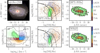 |
Fig. 3. Same as Fig. 2, corresponding to the eCALIFA data of NGC 2906. |
| In the text | |
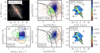 |
Fig. 4. Same as Fig. 2, corresponding to the eCALIFA data of NGC 6286. |
| In the text | |
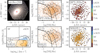 |
Fig. 5. Same as Fig. 2, corresponding to the eCALIFA data of NGC 3610. |
| In the text | |
Current usage metrics show cumulative count of Article Views (full-text article views including HTML views, PDF and ePub downloads, according to the available data) and Abstracts Views on Vision4Press platform.
Data correspond to usage on the plateform after 2015. The current usage metrics is available 48-96 hours after online publication and is updated daily on week days.
Initial download of the metrics may take a while.