| Issue |
A&A
Volume 673, May 2023
|
|
|---|---|---|
| Article Number | A70 | |
| Number of page(s) | 38 | |
| Section | Atomic, molecular, and nuclear data | |
| DOI | https://doi.org/10.1051/0004-6361/202142570 | |
| Published online | 10 May 2023 | |
Simulation of CH3OH ice UV photolysis under laboratory conditions
1
Laboratory for Astrophysics, Leiden Observatory, Leiden University,
PO Box 9513,
2300
RA Leiden,
The Netherlands
e-mail: This email address is being protected from spambots. You need JavaScript enabled to view it.
2
Niels Bohr Institute & Centre for Star and Planet Formation, University of Copenhagen,
Øster Voldgade 5-7,
1350
Copenhagen K.,
Denmark
3
Space Research Institute, Austrian Academy of Sciences,
Schmiedlstrasse 6,
8042
Graz,
Austria
4
Instituto de Pesquisa e Desenvolvimento (IP&D), Universidade do Vale do Paraíba,
Av. Shishima Hifumi 2911,
CEP 12244-000,
São José dos Campos, SP,
Brazil
5
Max-Planck-Institut für extraterrestrische Physik,
Giessenbachstrasse 1,
85748
Garching,
Germany
6
Max Planck Institute for Astronomy,
Königstuhl 17,
69117
Heidelberg,
Germany
7
Kapteyn Astronomical Institute, University of Groningen,
The Netherlands
Received:
2
November
2021
Accepted:
8
February
2023
Abstract
Context. Methanol is the most complex molecule that is securely identified in interstellar ices. It is a key chemical species for understanding chemical complexity in astrophysical environments. Important aspects of the methanol ice photochemistry are still unclear, such as the branching ratios and photodissociation cross sections at different temperatures and irradiation fluxes.
Aims. This work aims at a quantitative agreement between laboratory experiments and astrochemical modelling of the CH3OH ice UV photolysis. Ultimately, this work allows us to better understand which processes govern the methanol ice photochemistry present in laboratory experiments.
Methods. We used the code ProDiMo to simulate the radiation fields, pressures, and pumping efficiencies characteristic of laboratory measurements. The simulations started with simple chemistry consisting only of methanol ice and helium to mimic the residual gas in the experimental chamber. A surface chemical network enlarged by photodissociation reactions was used to study the chemical reactions within the ice. Additionally, different surface chemistry parameters such as surface competition, tunnelling, thermal diffusion, and reactive desorption were adopted to check those that reproduce the experimental results.
Results. The chemical models with the code ProDiMo that include surface chemistry parameters can reproduce the methanol ice destruction via UV photodissociation at temperatures of 20, 30, 50, and 70 K as observed in the experiments. We also note that the results are sensitive to different branching ratios after photolysis and to the mechanisms of reactive desorption. In the simulations of a molecular cloud at 20 K, we observed an increase in the methanol gas abundance of one order of magnitude, with a similar decrease in the solid-phase abundance.
Conclusions. Comprehensive astrochemical models provide new insights into laboratory experiments as the quantitative understanding of the processes that govern the reactions within the ice. Ultimately, these insights can help us to better interpret astronomical observations.
Key words: astrochemistry / ISM: molecules / solid state: volatile
© The Authors 2023
 Open Access article, published by EDP Sciences, under the terms of the Creative Commons Attribution License (https://creativecommons.org/licenses/by/4.0), which permits unrestricted use, distribution, and reproduction in any medium, provided the original work is properly cited.
This article is published in open access under the Subscribe to Open model. This email address is being protected from spambots. You need JavaScript enabled to view it. to support open access publication.
1 Introduction
Methanol (CH3OH) ice has been securely detected in the interstellar medium (ISM) towards different lines of sight (e.g. Schutte et al. 1991; Chiar et al. 2000; Pontoppidan et al. 2004; Boogert et al. 2011; Perotti et al. 2020, 2021; Chu et al. 2020; Goto et al. 2021; Kim et al. 2022). We highlight the recent detection made with James Webb Space Telescope (JWST) observations towards the class 0 protostar IRAS 15398-3359 (program 2151, PI: Y.-L. Yang; Yang et al. 2022) and in the densest regions of the molecular clouds Chameleon I (McClure et al. 2023) as part of the Early Release Science (ERS) Ice Age program (PIs: M. Mcclure, A. Boogert, and H. Linnartz). This simple alcohol is mostly formed via successive CO hydrogenation (Watanabe & Kouchi 2002; Fuchs et al. 2009) through so-called dark ice chemistry (Ioppolo et al. 2021), a term that is used to characterize molecular synthesis without the influence of ionizing radiation. Additionally, other surface reactions at low temperature have been proposed in the literature. Qasim et al. (2018) found experimentally that CH3OH is formed via a sequential surface reaction chain at low temperature, that is, CH4 + OH → CH3 + H2O and CH3 + OH → CH3OH. More recently, Santos et al. (2022) confirmed via experiments that CH3OH also forms in the ice via CH3O + H2CO → CH3OH + HCO at temperatures similar to the interior of molecular clouds. Additionally, methanol ice is formed by energetic processing of simple molecules in the ice mantle, such as H2O, CO and CO2 (e.g. Jiménez-Escobar et al. 2016). Despite its low abundance towards low-mass star-forming regions (5–12% with respect to H2O ice; Öberg et al. 2011), methanol is crucial for understanding the chemical complexity in stellar nurseries because it is the precursor of large and complex organic molecules (COMs; Öberg et al. 2009a; Öberg 2016). In the Solar System, methanol has also been detected in comets (e.g. 67P/Churyumov-Gerasimenko; Le Roy et al. 2015) and Kuiper belt objects (e.g. Grundy et al. 2020). In the former, mono- and di-deuterated methanol detection in a cometary coma has also been reported by Drozdovskaya et al. (2021). In the latter case, spectral analysis of Arrokoth suggests a water-poor surface and a high abundance of methanol (Grundy et al. 2020).
In order to provide qualitative information on how frozen methanol promotes the synthesis of COMs, systematic laboratory experiments simulating the effects of UV radiation on the CH3Oh ice were performed by Öberg et al. (2009a). From that study, the formation of several COMs such as CH3CH2OH, CH3OCH3, HCOOCH3, and HOCH2CHO was observed. As suggested by the authors, this is the result of CH3OH photolysis and radical recombination after diffusion. Nevertheless, a few aspects remained unclear, such as the reaction channel that dominates at different temperatures and fluences (flux integrated over time), as well as the branching ratios (BRs), that is, the fraction of the radicals formed after UV photolysis. Additionally, the photodissociation cross sections derived from this experimental study are underestimated because of the immediate methanol ice re-formation. Complementary chemical kinetic modelling is therefore necessary to completely quantify the photochemistry of methanol ices, as pointed out by the authors.
Combining careful modelling of ices under laboratory conditions aided by experiments might provide a comprehensive understanding of the processes that govern reactions within the ices. With this goal, Shingledecker et al. (2019) studied the proton-irradiation of O2 and H2O ices using astrochemistry-type models implemented with the code MONACO (Vasyunin et al. 2017), which uses a multiphase Monte Carlo approach to calculate chemical abundances in the context of gas-grain interaction. The models demonstrated that cosmic-ray-driven chemical reactions can reproduce the abundances of O2, O3, and H2O2 observed in the experiments if the radicals produced by protonirradiation react quickly and locally in the ice. Similarly, the formation of S8 and other sulfur-bearing species was addressed with the same method by Shingledecker et al. (2020), who again showed that these kinetic studies of chemical reactions in the ices agree with the abundances of sulfur-bearing species measured towards comet 67P/C-G by the ROSINA instrument (Rosetta Orbiter Spectrometer for Ion and Neutral Analysis; Balsiger et al. 2007) on ESA's Rosetta mission (Calmonte et al. 2016). In a lower-energy regime, Mullikin et al. (2021) successfully simulated the ozone (O3) formation due to UV irradiation of O2 ice using a Monte Carlo-based model. In their simulations, chemical processes such as photoionization, photoexcitation, and the formation of electronically excited species were considered in the models. Despite the good agreement between experiments and simulations, the caveats in these approaches are the uncertainties in the chemical networks, the reaction rates, and the BRs for surface chemistry processes included in the models. Further theoretical works exploring these uncertainties and using a reduced network have been carried out by Pilling et al. (2022), Carvalho et al. (2022), and Pilling et al. (2023), aiming at the determination of effective rate constants of reactions in the solid phase.
Inside dense molecular clouds, energetic cosmic rays excite the gas-phase H2, which results in Lyman and Werner emission lines (Prasad & Tarafdar 1983). These are the secondary UV photons. The typical flux in dense starless cores ranges from 103 to 104 cm−2 s−1 (e.g. Shen et al. 2004). Although it represents a mild flux, over the timescale of molecular clouds (<10 Myr; e.g. Clark et al. 2012), this results in fluence of around 1018 cm−2. This is comparable with the fluence adopted by Öberg et al. (2009a) to photolyse the methanol ice and to form a variety of COMs. Additionally, other laboratory experiments with UV as an irradiation source have reported the formation of prebiotic molecules, such as ribose (Meinert et al. 2016) and deoxyribose (Nuevo et al. 2018). In spite of the importance of chemical processes within ices triggered by UV radiation, little is known about these processes. In addition, the JWST is dedicating many hours to observe ices, which makes it crucial to improve our understanding of the mechanisms involved in ice photolysis. To shed light on this problem, and to shrink the gap between laboratory and chemical models, we introduce in this paper systematic modelling of methanol ice photochemistry triggered by UV radiation using the code ProDiMo (Woitke et al. 2009; Kamp et al. 2010; Thi et al. 2011), which is currently equipped with surface chemistry (Thi et al. 2020a,b). In particular, we have modelled the methanol ice destruction under laboratory conditions shown in Öberg et al. (2009a). When the best results are found, they are used to simulate the chemical evolution in a molecular cloud environment. The differences and similarities in the models with or without methanol ice photochemistry are discussed.
This paper is outlined as follows. Section 2 introduces the chemical model used to reproduce the methanol UV photolysis. In Sect. 3, the set-up of the models considering different surface chemistry parameters is presented and the best model is selected. The results of this study are shown in Sect. 4, and Sect. 5 is focused on the discussion and astrophysical implications.
2 Chemical model
Our two-phase chemical model was constructed with the code ProDiMo, which originally is a thermochemical radiative transfer code for modelling the physics and chemistry of protoplanetary disks and molecular clouds. In particular, we have used the surface chemistry module, recently developed by Thi et al. (2020a,b). We changed the setup of these models to simulate the radiation fields, pressures, composition, and thickness of ice layers as they are prepared in laboratory experiments. Regarding the surface chemistry processes, the models include photolysis (photodissociation) with different BRs, thermal and non-thermal desorption, and diffusion mechanisms via tunnelling and thermal hopping. Further details about these parameters and processes are given in the next subsections.
2.1 UV flux
The experiment performed by Öberg et al. (2009a) used UV irradiation to destroy the methanol ice in their experiments. In ProDiMo, the chemical models adopt a UV flux as a function of the values in the ISM. The standard UV radiation field in the ISM in units of erg cm−3 is formally defined by Draine (1978) and Draine & Bertoldi (1996),
 (1)
(1)
where λ is the wavelength,  is the spectral photon energy
  , c is the speed of light, Jλ is the mean intensity, and λ3 = λ/100 nm. The standard Far-UV (FUV) flux of the ISM is found by integrating Eq. (1) between 91.2 nm and 205 nm,
![Mathematical equation: $\matrix{ {{F_{{\rm{Draine}}}} = {1 \over h}\int_{91.2\,\,{\rm{nm}}}^{205\,\,{\rm{nm}}} {\lambda u_\lambda ^{{\rm{Draine}}}{\rm{d}}\lambda } } \hfill \cr {\,\,\,\,\,\,\,\,\,\,\,\,\,\,\, = 1.9921 \times {{10}^8}\,\,\left[ {{\rm{c}}{{\rm{m}}^{ - 2}}{{\rm{s}}^{ - 1}}} \right],} \hfill \cr }$](/articles/aa/full_html/2023/05/aa42570-21/aa42570-21-eq4.png) (2)
(2)
where h is Planck's constant. The integration interval spans over crucial physical processes such as (i) the photoexcitation and photodissociation of many molecules including H2, (ii) photoionization of heavy elements, and (iii) the ejection of electrons from dust grains. The FUV radiation strength (χ) of local regions in the ISM is frequently normalized by the radiation field from Draine, and it is given by
 (3)
(3)
where Fλ is the local FUV flux. By definition, the strength of the standard FUV flux in the ISM is χISM = 1.
In laboratory experiments, the UV radiation is produced by H2 or D2 microwave discharge lamps. The spectrum usually covers 110–180 nm and is characterized by a strong Ly α peak at 121 nm and fluorescence emission around 160 nm. As found by Ligterink et al. (2015), the Ly α peak intensity can be increased and the fluorescence decreased if helium (He) is added with H2 or D2, respectively.
Figure 1 compares the UV spectra in the laboratory and ISM. The typical laboratory UV flux integrated from 110 nm to 200 nm is around 1012–13 cm−2 s−1, that is, four or five orders of magnitude higher than the typical ISM value (see Eq. (2)). Because of this difference, it is postulated in the literature that a high flux in the laboratory in a short period of time produces the same chemistry as in the ISM, which has a low flux over a longer period. This can be translated into the term 'fluence', which means the flux integrated over time. As a test case, Öberg et al. (2009a) compared two experiments with different fluxes (factor of four difference), but with the same fluences. As the authors observed, the IR spectra are identical within the experimental uncertainties. In this paper, we used χ = 5 × 10⁴ to simulate the UV flux of 1.1 × 1013 cm−2 s−1 used by Öberg et al. (2009a).
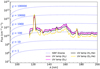 |
Fig. 1 Comparison between the UV flux distribution of the interstellar radiation field (χ) from Draine (1978) and from the lamps used in the laboratory for ice photochemistry. |
2.2 Pump simulator
In laboratory experiments with astrophysical ices, high or ultrahigh vacuum conditions are required to avoid (i) atmospheric contamination and (ii) re-condensation of the photoproducts that are released to the gas phase, and to control the evolution of the ice composition. The typical vacuum inside the experimental chamber is around 10−10 mbar, which is usually achieved by combining diffusion and turbo-molecular pumps.
In our model, the gas pressure is calculated by the following equation:
 (4)
(4)
where ntot is the total gas density, kB is the Boltzmann constant, and Tg is the gas temperature. To simulate the same laboratory conditions, an initial pressure of 10−10 mbar due to the residual gas (e.g. He) is assumed.
During the simulations, the gas pressure increases because of the chemical species that migrate from the ice to the gas phase. To maintain constant pressure, a correction factor f of around 0.01 is often applied to Eq. (4).
2.3 Surface chemistry
Simulating the chemical reactions within the ices under laboratory conditions with astrochemical-type models is challenging and inevitably introduces caveats. For example, the grain surface chemistry in ProDiMo assumes that ices mantles are formed on a dust grain, whereas in the laboratory, ices are condensed on a plain substrate (e.g. CsI, ZnSe, and KBr), which leads to differences in the binding energies in the interface between substrate and molecule and grain and molecule. However, this effect is minimized for thick ice layers, where the chemical species are mostly bound by van der Waals forces. In the models, the majority of the ice chemistry occurs in the statically well-mixed mantle, where all adsorptions and desorptions are on physisorption sites (see Sect. 2.3.3). There is no distinction between ice surface and bulk. However, the ice chemistry itself in ProDiMo is considered multi-phase because of the chemistry that can occur in the ice mantle (phase 1), interface mantle and core (phase 2), or in the core itself (phase 3), where only chemisorption sites are considered.
In this subsection, we describe the details of the chemical network adopted in our models, as well as the surface chemistry parameters we have adopted to simulate the methanol ice photolysis. These parameters include photodissociation, radical migration, and thermal and non-thermal desorption mechanisms. The different models with or without these processes are described in Sect. 2.4.
2.3.1 Network and branching ratios
Both gas- and solid-phase reactions are included in the network of chemical reactions considered in this paper to model the methanol ice photodissociation. If not explicitly discussed, the chemical reaction pathways and their rates are taken from the KIDA database, kida.uva.2014. Appendix B lists the gas and ice chemical species used in this work. Appendix C contains the list of newly added surface photolysis, and Appendix D shows the bimolecular surface reactions and binding energies used in this paper, cross-checked against Wakelam et al. (2017). We highlight that we assumed the binding energy as a single value, and not as a distribution as discussed by Shimonishi et al. (2018), Grassi et al. (2020), Bovolenta et al. (2022), Villadsen et al. (2022), and Minissale et al. (2022). In addition to the methanol formation and destruction pathways included in these lists, we added the methanol ice photodissociation routes (see Table 1).
Currently, there is no consensus about the methanol ice BRs. The standard BRs used in astrochemical models were proposed by Garrod et al. (2008) and assume a destruction channel favouring the methyl channel (CH3) for the gas phase and solid phase. Although the overall rate coefficient for methanol photodissociation used in the Garrod et al. (2008) models was derived from gas-phase experimental work, the BRs are not constrained by laboratory work. A measurement of this in the ice phase was carried out by Öberg et al. (2009a) using infrared (IR) and mass spectrometry analysis. In contrast to the previous BRs proposed by Garrod et al. (2008), the experiments demonstrated that solid-phase methanol is mainly destroyed via the hydroxymethyl (CH2OH) channel.
By using rate-equation-based chemical models, Laas et al. (2011) addressed the impact of the BRs in the production of complex molecules observed towards Sgr B2(N). In addition to the standard BRs proposed previously, another two values were also adopted to test extreme cases in which CH3, CH2OH, or OCH3 is the dominant channel of destruction. It was observed that for some COMs, CH3 or OCH3 agrees better with the gas-phase observations. Conversely, the CH2OH channel matches less well, which is in contrast to the experimental results found by Öberg et al. (2009a).
More sensitive measurements in the ice phase were made by Paardekooper et al. (2016) using time-of-flight mass spectrometry analysis. Initially, the authors traced the abundance of the photoproducts CH2OH, CH3, and OCH3 to follow the chemical network proposed by Öberg et al. (2009a). Next, the abundance of new molecules formed by the recombination of the photoproducts was investigated. Only OH-dependent species were excluded from this tracking because of water formation during the experiments, which is an important sink for the hydroxyl (OH) radical. The BR deduced from this analysis indicates that the CH2OH branch is the dominant photodestruction route of methanol ice. While this result qualitatively agrees with the BRs found by Öberg et al. (2009a), the experiments showed 35% more icy methanol destruction via the CH3 channel and ~5% less destruction via the CH2OH channel.
A different technique was used by Weaver et al. (2018) to estimate the methanol photolysis BRs in the gas phase. In a vacuum chamber, methanol was photodissociated by a VUV laser in the throat of a supersonic expansion. After this, the products were analysed with millimeter and submillimeter spectroscopy to derive abundances in the gas phase. This study showed the same photoproducts as were observed in the experiments by Öberg et al. (2009a) and Paardekooper et al. (2016), with the addition of formaldehyde (H2CO), which was not observed in the experiments in the solid phase as a direct photoproduct of the methanol ice. However, this agrees with Hagege et al. (1968), who identified H2CO as one of the photoproducts of gaseous methanol.
Finally, an experiment performed by Yocum et al. (2021) suggested that the OCH3 radical is the dominant branch of the methanol ice photolysis. The study was carried out by combining solid-phase analysis using standard IR spectroscopy and submillimeter/far-IR spectroscopy when the ice was warmed up to 300 K. However, no quantification of the BRs was estimated.
The percentage values of these different BRs of methanol ice photodissociation are summarized in Table 1. They are explored in this paper along with other parameters detailed in this section to find the best solution that matches the experimental data.
Branching ratios of methanol ice photodissociation.
2.3.2 Photodissociation
The absorption of UV photons by a molecule in the ice changes its energy state to an excited level, which might lead to molecular fragmentation. However, the dissociation probability decreases as the number of atoms in the molecule increases because of the high number of vibrational modes (Bixon & Jortner 1968; Tramer & Voltz 1979; Leger et al. 1989; van Dishoeck & Visser 2011). When a photon is absorbed by a large molecule, the internal vibrational energy is rapidly redistributed, and the molecule ends up at a highly excited vibrational level. Subsequently, the molecule relaxes by emission of IR photons or fluorescence before arriving at the electronic ground state. The probability that the molecule finds a path to dissociation is rather low. For example, experiments performed by Jochims et al. (1994) showed that the photostability of polycyclic aromatic hydrocarbons is significantly reduced when the number of atoms is lower than 30–40. For small and intermediate-sized molecules containing fewer than ten atoms (including CH3OH), Ashfold et al. (2010) concluded from theoretical work that their dissociative excited states are comparable to those of H2O and NH3, regardless of the level of structural complexity.
In laboratory conditions, the FUV flux is not dependent on the visual extinction (AV), and the photodissociation rate is equal to the photorate α calculated in Appendix A, that is,
![Mathematical equation: $R_i^{{\rm{phd}}} = \bar \sigma \cdot {F_{{\rm{lamp}}}}\,\,\,\,\left[ {{{\rm{s}}^{ - 1}}} \right],$](/articles/aa/full_html/2023/05/aa42570-21/aa42570-21-eq7.png) (5)
(5)
where  is the average photodissociation cross section (unit cm−2) measured in the laboratory adopting an H2 (or D2) lamp as the UV source with flux Flamp. The flux lamp can be scaled to the strength of the FUV field from Draine by Flamp = χFDraine. Equation (5) becomes
 ![Mathematical equation: $R_i^{{\rm{phd}}}\left[ {{{\rm{s}}^{ - 1}}} \right] = \bar \sigma \cdot 1.9921 \times {10^8}$](/articles/aa/full_html/2023/05/aa42570-21/aa42570-21-eq9.png) when χ = 1.
when χ = 1.
2.3.3 Chemisorption, physisorption, and diffusion
Two potential energy regimes keep chemical species stuck on the catalytic surface: chemisorption (c), and physisorption (p). In the former case, short-range forces associated with the overlap of the wave functions promote strong bonds between the grain surface and the first ice layers above. In the latter case, large distance forces take place, and the attraction due to the van der Waals force promotes weak binding at upper ice layers. It is worth noting that the binding energies in the two cases are vastly different as well. In computational modelling, the physisorption sites only become available after the chemisorption sites are filled.
In this model, atoms and molecules can diffuse by changing states (physisorption or chemisorption), and they can migrate from physisorption to chemisorption sites and vice versa. The probability of overcoming an adsorption activation barrier for chemisorption is described by the tunnelling-corrected Arrhenius formula, called Bell's formula (Bell 1980; Bell & Le Roy 1982), namely, QBell, which is given by
 (6)
(6)
where ai is the width of the rectangular activation barrier of height Ei, mi is the mass of the atoms or molecule, and Tg is the gas temperature, assumed here to be equal to the dust temperature (Td). The parameters α and β are defined as
 (7)
(7)
and
 (8)
(8)
Finally, the diffusion rate is given by
 (9)
(9)
where  is the vibrational frequency of the species in the surface potential well of ice species i, Ts is the surface temperature, nbsite is the number of adsorption sites per ice monolayer equal to 4πNsurf a2, and ΔEif is the energy difference between the sites i and f. Nsurf is the surface density of adsorption sites, that is, 1.5 × 1015 cm−2, also known as the Langmuir number, and a2 is the grain radius squared.
As the chemical species are migrating over the catalytic surface, they can react via the Langmuir-Hinshelwood mechanism, following the rate
 (10)
(10)
where κij is the reaction probability of occurring after the species i and j have diffused, and it is formally defined a:
 (11)
(11)
in which  . The frequency ν is defined by the equation of a rectangular barrier given by
 (12)
(12)
where Ei is the height of the barrier, and Nsurf is the surface site density, which is equal to 1.5×10¹⁵ sites cm−2. In the cases of bar-rierless reactions and diffusion-limited conditions, that is, when only thermal hopping or diffusion tunnelling dominate, κij → 1. The energy barrier for H to migrate from one physisorbed site is not negligible, but ranges from 256 K (Kuwahata et al. 2015) to 341 K (Congiu et al. 2014), which allows H to recombine locally when radicals are abundant because of barrieless reactions (κij = 1) or after diffusion because the diffusion energy is around 30−50% of the desorption energy (e.g. Ruffle & Herbst 2000; Garrod et al. 2008; Thi et al. 2020a). The number of reactions per second (rate) is directly proportional to the number of species of the reactants that are available (ni, nj),
 (13)
(13)
On the other hand, if there is a surface competition between the two diffusion mechanisms, κij ≠ 1. For instance, in a surface competition scenario of H2, κij ≃ 1/3. Surface competition occurs when the surface reaction process competes with diffusion and desorption, as defined by Herbst & Millar (2008), Garrod & Pauly (2011), and Cuppen et al. (2017).
The gas-phase atom or radical recombination with an adsorbed species from the grain surface (Eley-Rideal reactions) are not considered in this paper. Additionally, the sticking coefficient of all molecules in the gas phase was deliberately set to zero to certify that molecules desorbing from the ice do not adsorb again. In this approach, is reasonable to ignore these processes to reach better agreement with the experimental conditions.
2.3.4 Desorption
The desorption mechanism is characterized by the release into the gas phase of a chemical species from the catalytic surface when its internal energy is greater than the binding energy with the sticking surface. In this model, three desorption pathways are considered.
Thermal desorption
The thermal desorption rates of chemical species in physisorption or chemisorption regimes are given by
 (14)
(14)
where  is the desorption energy, defined as the sum of the binding energy and the activation energy, that is,
  . In the physisorption regime,
  , whereas the chemisorption bonds require activation energy
  to be broken. The number of active surface places in the ice per volume subject to the thermal desorption is given by
 (15)
(15)
where <a2> is the squared mean grain size value, nd is the dust grain numerical density, Nsurf is the surface density of adsorption sites in one monolayer of ice, also known as the Langmuir number, and NLay is the number of surface layers considered as active. In the literature, the values attributed to NLay are 2 (Aikawa et al. 1996), 4 (Vasyunin & Herbst 2013), and 6 (Öberg et al. 2009a). In this paper, we assume NLay = 6 to be consistent with the experiments performed by Öberg et al. (2009a).
Photodesorption
The internal energy of a chemical species on the grain surface can be increased by the absorption of a UV photon, and the photodesorption of species i is given by
 (16)
(16)
where Yi is the photodesorption yield, and χ is the Draine field parameter. Generally, Yi depends on the ionizing source and the composition and thickness of the ice (e.g. Brown et al. 1984; Westley et al. 1995; Öberg et al. 2009b; Fayolle et al. 2011; Dartois et al. 2018). For pure CH3OH ice, Öberg et al. (2009a) found Yi = 10−3, whereas Bertin et al. (2016) found Yi = 10−5. Both values were tested in this paper.
Reactive desorption
Due to the exothermicity of some surface reactions, the bond between the chemical species and the surface is broken, thus resulting in non-thermal desorption, as experimentally confirmed by Dulieu et al. (2013). This mechanism was introduced into astrochemical models by Garrod et al. (2007), and the desorption probability (P) is quantified by the Rice-Ramsperger-Kessel (RRK) theory (e.g., Holbrook et al. 1996) and is defined as
![Mathematical equation: $P = {\left[ {1 - {{{E_{\rm{b}}}} \over {{E_{{\rm{reac}}}}}}} \right]^{s - 1}},$](/articles/aa/full_html/2023/05/aa42570-21/aa42570-21-eq27.png) (17)
(17)
where Eb is the binding energy of the product molecule, Ereac is the energy released in the formation, and s is the number of vibrational modes of the molecule/surface-bound system. When P is known, the fraction of reactive desorbed products is calculated by
 (18)
(18)
where e is an empirical parameter that relates the frequencies of molecule-surface bonds and of the energy transferred to the grain surface. The classical value adopted in the literature is 1% (e.g. Aikawa et al. 2008; Vasyunin & Herbst 2013; Shingledecker et al. 2020) because it provides better agreement with chemical abundances derived from astronomical observations. It is worth mentioning that molecular dynamic calculations indicate that a value higher than 1% is unlikely (Kroes & Andersson 2005), and a lower percentage cannot be rejected (Kristensen et al. 2010).
Another formalism has been proposed by Minissale et al. (2016), in which the fraction of reactive desorption depends on the substrate and the mass of the product. In this case, the fraction is given by
 (19)
(19)
where N is the number of degrees of freedom of the product species, and ϵ = [(M − m)/(M + m)]2 is the energy kept by the product of mass m on a surface of mass M.
2.4 Model set-up
To replicate the CH3OH ice photodissociation as measured by Öberg et al. (2009a), seven models considering different surface chemistry parameters described in Sect. 2.3 were adopted. Additionally, because the silicate core is not simulated in this work, the surface reactions were limited to the physisorption regime. A summary of each model is shown in Table 2. Thermal diffusion was considered in all models. Models 1 and 2 represent the scenarios with surface competition and diffusion/reaction tunnelling while adopting the approaches from Garrod et al. (2007) and Minissale et al. (2016), respectively. In models 3 and 4, the surface competition was switched off, but diffusion/reaction tunnelling to overcome the activation energy barrier in the two-body reaction was kept. This allowed us to assess the impact of surface competition in models 1 and 2. Similarly, in models 5–6, we enabled surface competition and switched off tunnelling for diffusion and reaction. In this way, the effect of diffusion/reaction tunnelling in models 1 and 2 were evaluated. Finally, model 7 represents a scenario in which only thermal diffusion and reaction desorption according to the approach of Garrod et al. (2007) were considered.
Each model listed in Table 2 was performed assuming temperatures of 20, 30, 50, and 70 K to mimic the experiments carried out by Öberg et al. (2009a). The experimental photodissociation cross sections of methanol ice calculated at these four temperatures are 2.6 ± 0.9 × 10⁻¹⁸ cm−2 at 20 K, 2.4 ± 0.8 × 10⁻¹⁸ cm−2 at 30 K, 3.3 ± 1.1 × 10⁻¹⁸ cm−2 at 50 K, and 3.9 ± 1.3 × 10⁻¹⁸ cm−2 at 70 K. However, because of the efficient methanol ice re-formation, these values are underestimated (Öberg et al. 2009a). Roncero et al. (2018) also found a similar trend in the cross section of methanol reaction in the gas phase with OH. They observed that the reactive cross section had a minimum value when the temperature was increased, and then increased again. In their case, they interpreted this trend as the formation of a CH3OH-OH complex that only disappears via tunnelling towards the products.
To confirm that the σhd that provides the best agreement with the experiments, the interval between the lower and upper bounds of photodissociation cross sections calculated by Öberg et al. (2009a) were used to create a grid of unshielded photorates (α) for different BRs listed in Table 1. Specifically, the lower and upper bound intervals of σhd are evenly spaced, and subsequently, the rates associated with each BRs (Table 1) were used in the simulations. A summary of the physical parameters adopted in the model set-up is given in Table 3. It also includes the size of the dust grain (α) that acts as the substrate in the experiments and the dust-to-gas ratio (δ) that was used in the simulations.
Surface chemistry parameters used in the set-up of seven models.
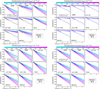 |
Fig. 2 Grid of methanol ice photodissociation in models 1 and 2 at 20 K (left panel) and at 30 K (right panel). The models assume different photodissociation cross sections and BRs (see Table 1). These models assume surface competition, diffusion, reaction tunnelling, and thermal diffusion. In addition, models 1 and 2 adopt the reactive desorption formalism from Garrod et al. (2007) and Minissale et al. (2016), respectively. |
Physical parameters used in the chemical simulation of CH3OH ice photolysis
3 Results
3.1 Grid of photodissociation curves
A grid of 1,120 photodissociation curves was simulated in order to find a good match with the experimental data. A series of photodissociation curves simulated with ProDiMo by adopting different BRs in models 1 and 2 at 20 K is shown in the left panels of Fig. 2, and the right panels shows the results when simulations were performed with temperature equal to 30 K. These curves show that the variation in the BRs and in the surface chemistry parameters leads to different results that may or may not fit the experimental data.
Despite the intrinsic differences among the models, we note that the reactive desorption from Minissale et al. (2016) promotes more destruction of the CH3OH ice than the mechanism from Garrod et al. (2007) at all four temperatures. Nevertheless, it is the only scenario in which the fits match the experiments at 30 K. The top right panel in Fig. 2 shows that the methanol ice photodissociation is rather underestimated at 30 K when the reactive desorption from Garrod et al. (2007) is adopted. On the other hand, the bottom right panels in Fig. 2 show that the models match the experimental data when reactive desorption from Minissale et al. (2016) is considered. We observed the repetition of this trend for the four temperatures addressed in this paper. An analysis of the chemical reactions that led to these results is reported in Sect. 4.1.
Appendix E shows the gallery of fits for models 3–7 at 20 K and 30 K and for models 1–7 at 50 K and 70 K, which are omitted in this subsection. To decide which case fits the experiments from all simulations best, we used the approach described in Sect. 3.2.
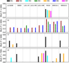 |
Fig. 3 Accuracy of the CH3OH ice photodissociation fit for models 1–7. Higher bars indicate the best models. When no bars are shown, the MLE values are lower than the y-axis threshold. The hatched and solid bars indicate the models assuming the reactive desorption mechanism by Minissale et al. (2016) and Garrod et al. (2007), respectively. |
3.2 BR selection
As most of the models can fit the experimental data in some scenarios, the best fit was selected based on two criteria: first, the maximum likelihood estimator (MLE), calculated by
![Mathematical equation: ${\rm{MLE}} \equiv \ln p\left( {\left. {{y^{{\rm{lab}}}}} \right|{y^{\bmod }}} \right) = - {1 \over 2}\sum\limits_i {\left[ {\left( {{{y_i^{\bmod } - y_i^{{\rm{lab}}}} \over {{\delta _i}}}} \right) + \ln \left( {2\pi \delta _i^2} \right)} \right]\,,}$](/articles/aa/full_html/2023/05/aa42570-21/aa42570-21-eq30.png) (20)
(20)
where ylab and ymod are the normalized methanol ice column densities from the laboratory and the model, respectively, and δi is the absolute error of the measurements. The second criteria is that  , as discussed by Öberg et al. (2009a).
Figure 3 shows the MLE values in a bar diagram for models 1–7 at four temperatures and different BRs. The higher values of MLE indicate the best model. The absent bars refer to models for which the best fit is obtained with  , which does not satisfy the second criterion. In all scenarios, the BR from Paardekooper et al. (2016) provides the best agreement with the experimental data. This suggests that methanol ice is mostly destroyed by the hydroxymethyl branch (CH2OH# + H#), not by the methyl and methoxy pathways. Concerning the reactive desorption mechanism, models adopting the reactive desorption formalism from Garrod et al. (2007) provide better fits at T = 20, 50, and 70 K, whereas at T = 30 K, the formalism from Minissale et al. (2016) agrees better with the data. As shown in the bottom left panel in Fig. 2 and Figs. E.6, E.8, and E.10 (Appendix E), none of the fits adopting reactive desorption from Garrod et al. (2007) can match the experimental data at 30 K.
Of the models adopting the BR from Paardekooper et al. (2016), model 1 always provides the best fit at 20 K, 50 K, and 70 K, whereas at 30 K, model 2 results in better agreement with the experiments. These two models both account for surface competition and diffusion/reaction tunnelling for migration and reaction on the grain surface. However, at 20 K, the difference among the MLE values in models 1, 3, 5, and 7 is smaller than 5%, thus suggesting that surface competition and diffusion/reaction tunnelling are not critical at this temperature. The same trend is observed at 30 K, where the difference between models 2, 4, and 6 is still smaller than 5%. Conversely, at 50 K, only model 1 provides a good match with the experiments, whereas at 70 K, model 1 is better than model 3 in 30%. This indicates that surface competition and diffusion/reaction tunnelling are essential for models at high temperatures.
Although the photodissociation curves adopting the Paardekooper BRs lead to better fits at the four temperatures, a few other cases also result in high fitness scores. For example, at 30 K, some models adopting the BRs from Weaver et al. (2018) can also fit the experiments well. At 50 K and 70 K, models considering other BRs also provide a relatively good match with the experiments. However, removing this degeneracy is not straightforward, and we decided to adopt the models providing the highest MLE value for the subsequent analysis in this paper.
3.3 Photodissociation rates
The methanol ice photodissociation rates were calculated using Eq. (5), which relates the integrated UV radiation field with the average photodissociation cross section. Based on the results shown in Fig. 3, the photodissociation cross sections based on the models are  ,
,  ,
,  , and
, and  . Although these values are about 10–15% higher than the experimental σpd, they indicate reasonable agreement, and the small σpd at 30 K is also obtained with the simulations. Table 4 shows the photorates of CH3OH ice with the Paardekooper et al. (2016) BR and at four temperatures. Again, at 30 K, the photorate of the path CH3OH# + hv → CH3# + OH# is one order of magnitude lower than the cases at 20, 50, and 70K.
As pointed out by Öberg et al. (2009a), a likely reason for the 10–15% higher photodissociation cross section in the simulations is that methanol can still be re-formed locally because of the so-called cage effect (Franck & Rabinowitsch 1934). It states that the diffusion of the radicals formed during photolysis is inhibited because of the surrounding molecules. Consequently, fast recombination of the radicals occurs at the site of the photodissociation. In the case of pure CH3OH, CO and H2O ices, Laffon et al. (2010) showed that back reactions limit the destruction effect.
Methanol ice photodissociation pathways and unshielded photorates ( ) taken from the best models.
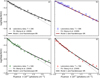 |
Fig. 4 Natural logarithm of the normalized CH3OH ice column density as a function of the UV fluence at 20, 30, 50, and 70 K in panels a–d, respectively. The symbols show the laboratory data from Öberg et al. (2009a), and the lines indicate the models that match the experiments best. |
3.4 Methanol ice destruction
Figure 4 shows the methanol ice destruction simulated with the code ProDiMo compared with the laboratory measurements at four temperatures during the first half-hour of the experiment. The photodissociation rates used in the simulations are shown in Table 4. In this figure, the dashed grey lines are the fits performed by Öberg et al. (2009a) to calculate the σphd assuming an exponential decrease in initial ice column density, given by
 (21)
(21)
where Ν(φ) and N(0) are the ice column densities at fluence φ (flux × time) and at the beginning of the experiment, respectively.
Equation (21) provides a good match with the experiments at 20, 50, and 70 K for fluences below 1 × 10¹⁷ photons cm−2. However, at fluences higher than 2 × 10¹⁷ photons cm−2, this exponential function overestimates the ice destruction, which might indicate methanol ice re-formation. A combination of exponential and linear analytical functions was used by Öberg et al. (2009a) to fit the ice destruction. They are associated with bulk photolysis and photodesorption, respectively. In contrast, the ice loss at 30 K is fully fitted by Eq. (21), which poses the question whether the methanol photodissociation at this temperature follows the same process at other temperatures.
In order to compare the ProDiMo results with the experiments, the normalized ice column density was calculated by the following equation:
 (22)
(22)
where n(φ) and n(0) are the respective numeric densities of methanol ice at fluence φ and at the beginning of the experiment. The same for the ice thickness d(φ) and d(0) is given by Eq. (15).
The models simulated with ProDiMo can reproduce the experimental measurements at the entire fluence range and four temperatures, as shown in Fig. 4. In all cases, model M1 resulted in better fits at 20 K, 50 K, and 70 K, whereas model M2 fits the data at 30 K. Models M1 and M2 include surface competition, diffusion/reaction tunnelling, and thermal diffusion, which indicates that these surface chemistry processes may occur within the ice during the photolysis. The difference between them is the reactive desorption formalism, as shown in Table 2. Additionally, these models assume BRs from Paardekooper et al. (2016). Figure 4 also shows that the simulations and the trend of the normalized column density values at all four temperatures agree well, which was not possible by using Eq. (21). This highlights that methanol ice is indeed re-formed more efficiently at 20, 50, and 70 K for fluences above 1×10¹⁷ photons cm−2. On the other hand, an additional methanol destruction route occurs in the experiment at 30 K. Below, we comment on the reason that models M2–M7 do not fit the data.
20K At this temperature, the models assuming reactive desorption via the Minissale et al. (2016) formalism, that is, M2, M4, and M6, always intensify the photodestruction of the methanol ice and cannot fit the experimental data. In this case, we comment on models M3, M5, and M7, which adopt the same reactive desorption efficiency as model M1. When surface competition is switched off (M3), the MLE is only 2% lower than in model M1, which indicates that diffusion may still occur in the ice. The lower agreement in model M5, in which no tunnelling is considered, shows that at low temperatures, this effect is strong. Finally, model M7, which does not account for surface competition and tunnelling, agrees least well with the experiments.
30K Different from the cases at 20, 50, and 70 K, the data at 30 K are only fitted by models M2, M4, and M6, where M2 produces the best fit. The surface competition is switched off in model M4, and methanol ice is slightly less strongly destroyed than in model M2. We found the same result in model M6, in which no diffusion and reaction tunnelling occur.
50K Similarly to the cases of 20 K, models M2, M4, and M6 enhance the photodestruction of methanol ice. On the other hand, models M3, M5, and M7 cannot induce enough photolysis in the ice. Model M3 does not consider surface competition, and methanol ice is more efficiently re-formed than expected from the experiments. The effect of tunnelling diffusion and reaction halts in model M5. We note that even though methanol ice is more thoroughly destroyed than in model M3, the photodissociation cross section to fit the data is higher than the upper limit estimated by Öberg et al. (2009a), which does not satisfy the goodness criteria we defined in Sect. 3.2. Finally, model M7 also shows that methanol is more efficiently re-formed than expected.
70K Again, models M2, M4, and M6 promote efficient photodestruction of the methanol ice beyond what is expected at 70 K. When surface competition is disabled in model M3, methanol ice is efficiently re-formed and cannot fit the experiments. When tunnelling is switched off in model M5, the methanol ice is more thoroughly destructed. A similar result is found with model M7.
3.5 Growth curves of the photoproducts
The photolysis of ices leads to the formation of several daughter species as evidenced by in situ analysis of laboratory experiments (see the review by Öberg 2016). The growth curves of some chemical species calculated with ProDiMo are compared with the experimental measurements in Fig. 5 at four temperatures. The growing curves of products formed just after irradiation (first generation) are different from products that formed after radical migration and reaction (second or more generations). In addition, the formation curve of molecules that formed from dissociation of first- or second-generation photoproducts is different again. Temperature is another physical parameter that can modify the growth curve because of the diffusion of the chemical species that are synthesized during the ice photolysis.
Figures 5a–d show the cases of CH2OH ice. This first-generation radical formed efficiently by the methanol ice photolysis. The experimental data indicate that the hydroxymethyl ice abundance with respect to the initial methanol column density is about 1% at 20, 30, 50 K, and 70 K. A good match is seen with the ProDiMo models at 20 and 30 K, whereas a difference of about one order of magnitude is observed at 50 and 70 K. As shown in reaction R1, hydroxymethyl is also formed via two-body reactions, and the mismatch between measurement and modelling can be associated with inaccuracies in the rates involved in this reaction at high temperatures.
Figures 5e–h show the cases of CO ice. The experimental abundance with respect to the initial methanol column density is about 1% at 20, 30, and 50 K, but it is not detected at 70 K. Because the desorption temperature of pure CO ice was calculated at about 20–25 K (Collings et al. 2004; Acharyya et al. 2007), its presence at 30 and 50 K is likely due to molecular migration into the porous ice matrix and thus is desorbed at a higher temperature. The models were not able to reproduce the experiments at any temperature. However, the difference between the simulated growing curve and the experiment at 20 K is smaller than in the cases at 30 and 50 K. The higher difference at 30 and 50 K (3 and 7 order of magnitude, respectively) can be explained by the lack of physical modelling with ProDiMo of the ice structure. On the other hand, the small difference at 20 K is likely due to inaccuracies in the reaction rates in the network, as in the case of hydroxymethyl. For example, during the methanol ice photodissociation, the CO ice is formed from the destruction of second-generation molecules,
 (R1)
(R1)
 (R2)
(R2)
 (R3)
(R3)
The CO2 ice formation is shown in Figs. 5i–l. It is mostly formed via OH# + CO# → CO2# + H#, and O# + HCO# → CO2# + H# at 20 and 30 K. At 50 and 70 K, reaction OH# + CO# → CO2# + H# is the main formation pathway of carbon dioxide. These reactions depend on the CO and HCO ice formation (reactions 1–3) and the OH photoproduct. A relatively good fit is observed at 30 and 50 K. At 20 K, the abundance from the model is one order of magnitude lower than the experiments, whereas at 70 K, the abundance of CO2 ice is seven orders of magnitude lower. Methane is also formed late because it depends on the photodissociation of two molecules, as already described. In the models shown in Figs. 5m–p, only the CH4 formation at 20 K is well reproduced. At 30, 50, and 70 K, the methane abundance is more than three orders of magnitude lower than measured in the experiments. Its formation indicates efficient diffusion of the radicals to the ice matrix porous, where they can react to form methane.
The formation pathways of HCO ice shown in Figs. 5q–t change with the temperature. At 20 and 30 K, they are formed via two-body reactions of H# + CO# → HCO#. There are different activation energies in the literature for this reaction. For this reason, we checked the differences assuming ΔΕ = 520 K (Fuchs et al. 2009), 1106 K (Rimola et al. 2014), and 2000 K (Awad et al. 2005). We note that the HCO# abundances in model M1 with a lower activation energy are srelatively close to the experimental results at 20 K, but the increase in the abundance is not significant at 30 K. Additionally, higher activation energies increase the mismatch. At 50 and 70 K, the reaction H2CO# + OH# → HCO# + H2O# dominates any other reaction. A good match with the experiments is found only at 50 K. Since the reaction H# + CO# is irrelevant, the growth curves are the same, regardless of the adopted activation energy. H2CO formation is shown in Figs. 5u–x. In the models presented in this paper, it is formed via photolysis of the methoxy radical, CH3O# + hν → H2CO# + H#. The photodissociation rate of this reaction is assumed to be 1 × 10⁻⁹ s−1 and might overestimate the methoxy photodissociation.
The mismatch between the model and experiments indicates not only that further laboratory studies are necessary to accurately reproduce surface reactions, but also that improvements of the models are needed. For example, chemical models including a more realistic energy redistribution when absorbing UV photons could provide useful insights into this framework. In the models shown in this paper, some differences are rather notable. At 20 K, the chemical abundances of some molecules and radicals in the models are lower measured from the experiments by one order of magnitude, except for the cases of CH2OH, HCO, and CH4. At 30 K, except in the cases of CH2OH and CO2, the abundances can be 2–5 orders of magnitude lower than measured by Öberg et al. (2009a). At 50 K, the abundances of CO, CH4, and H2CO are underestimated by two to several orders of magnitude. At 70 K, the models do not reproduce the measurements in any case.
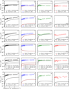 |
Fig. 5 Formation curves of selected daughter species (CH2OH, CO, CO2, CH4, HCO, and H2CO) due to CH3OH photolysis over fluence with respect to the initial methanol ice column density at four temperatures. The symbols are the experimental measurements, and the solid lines are the results of ProDiMo simulations of the best photodissociation models (see Fig. 4). |
4 Discussion
4.1 Chemical pathways at different fluences and temperatures
The most efficient chemical pathways to form and destroy methanol ice can be addressed by analysing the curvature in the molecule formation plots 20, 50, and 70 K (see Fig. 4) and the absence of this trend at 30 K. In this regard, the chemical reactions at fluences of 0.5, 1.5, and 2.4 × 10¹⁷ photons cm−2 were analysed.
For the four temperatures and selected fluences, methanol ice photodissociates following the pathways and branch ratios shown in Table 4. This indicates that bulk ice photolysis dominates other destruction processes either at the beginning of the experiment or after half an hour of constant irradiation in the case of thin ices (20 monolayers). We noted that the photodesorption mechanism is not significant at this range of fluence, regardless of whether the yield is Y = 10−3 or Y = 10−5. At 50 K and 70 K, methanol ice is further destroyed via a two-body surface reaction (Esplugues et al. 2016),
 (R4)
(R4)
where the activation barrier of this reaction is equal to 1000 K and makes reaction R4 inefficient at low temperatures. This reaction leads to the formation of H2O ice, which is one of the products observed from the experiments (Öberg et al. 2009a). At 20 K and 30 K, water ice is formed via the two-body reaction between H# + OH# and CH4# + OH# → CH3# + H2O#. CH4# readily forms via two-body reaction in the ice (CH3# + H# → CH4#). These pathways might explain the H2O ice formation in the experiments with methanol ice.
The models with ProDiMo show that a fraction of methanol ice is immediately re-formed after photodissociation in each of the selected fluences. The three re-formation reaction pathways are
 (R5)
(R5)
 (R6)
(R6)
 (R7)
(R7)
The recombination rates of reactions R5–R7 as a function of temperature are shown in the top panel of Fig. 6. The rate is defined as the product of the rate coefficient by the particle density of the reactants (see Eq. (13)). The bottom panel of Fig. 6 shows the number density of radicals that are available for recombination. At all four temperatures, methanol ice recombines faster via reaction R5 than via reactions R6 and R7 due to the large amount of CH2OH#. The trend observed in reaction R5 agrees with the number densities of CH2OH# formed after photolysis. Additionally, less H# is available for recombination due to hydrogen desorption, as indicated by the grey symbols in the right y-axis in the top panel of Fig. 6. The lower recombination rate at 30 K is caused by the small methanol ice photolysis cross section, and, consequently, the photorates at this temperature. As a result, fewer photoproducts are available for recombination in the ice. The rate decreasing trend as a function of temperature is also observed for reaction R6 (H# + CH3O#). The lower rates are associated with the lower BRs for this reaction (13%; see Table 4). The BRs also explain the lower rate values for reaction R7 (OH# + CH3#), but a different behaviour is observed for the recombination reaction trend. At 20 K, the low methanol ice re-formation via this reaction is due to the efficient reaction between H# and CH3# to form CH4#. At 30 and 50 K, methane is less abundant in our models, which increases the number of CH3 and OH in the ice for re-formation of CH3OH#. Despite the low number density of CH3#, OH# is high enough to increase the recombination rate at 50 K. At 70 K, the CH3# desorbs from the ice, which significantly decreases the methanol ice re-formation via reaction R7. Additionally, at this temperature, CH3OH# and OH# react.
Despite the decreasing recombination rate with increasing temperature for reactions R5 and R6, Fig. 6 indicates that a fraction of H remains in the ice to recombine mostly with CH2OH# to re-form CH3OH# at all four temperatures. The methane ice formation in the experiments shown in Sect. 3.5 also indicates that H is present in the ice, and reacts with other species at all four temperatures (e.g. CH4# and HCO#).
The effect of the fluence in the recombination reactions R5–R7 is shown in Fig. 7. The re-formation reaction rates vary little over the selected fluences. On the other hand, a significant variation is noted with the temperature. At 20 K, reactions R5 and R7 increase little with the fluence, whereas reaction R6 remains almost constant. At 30 K, all recombination rates decrease with the fluence, which consequently intensifies the methanol ice destruction. At 50 K, frozen methanol is mostly re-formed via reaction R5 over the fluences, whereas the rates of reactions R6 and R7 are constant and decrease, respectively. Finally, at 70 K, the rates of reactions R5 and R6 are constant during the experiments, and virtually null for reaction R7.
Reactions R4–R7 are crucial for understanding the methanol ice destruction via photolysis, but they cannot explain the trend in the destruction curve in the experiment at 30 K for fluences above 1.5×10¹⁷ photons cm−2. To further investigate this trend at 30 K and determine why the methanol ice recombination rate decreases over fluence (Fig. 7), we analysed other chemical reactions involving the photoproducts. This analysis showed that only at 30 K are the photoproducts further desorbed from the ice to the gas phase via reactive desorption by a factor of two compared to the experiments at 20 K, 50 K, and 70 K. The reaction scheme at 30 K is given by
 (R8)
(R8)
 (R9)
(R9)
 (R10)
(R10)
where the reactive desorption formalism from Minissale et al. (2016) was assumed in this case. Conversely, at 20 K, 50 K, and 70 K, methanol ice recombination via two-body reactions (R5–R7) dominates the reactive desorption by a factor of three, where reactive desorption from Garrod et al. (2007) was adopted. At 30 K, other species also leave the ice via reactive desorption at a lower rate than for reactions R8–R10 and reduce the number of reactants that can re-form methanol in the ice, which are
 (R11)
(R11)
 (R12)
(R12)
 (R13)
(R13)
Nevertheless, it is unclear why reactive desorption from Minissale et al. (2016) is only required at 30 K. An inaccurate determination of the methanol column densities at this temperature might explain the lack of the curved profile at longer fluences. However, the right panels of Fig. 2 and Figs. E.6–E.10 show that only models adopting reactive desorption from Minissale et al. (2016) can fit the experimental data at 30 K, where no curvature in the destruction profile is observed.
Figure 8 shows the total methanol ice destruction and formation rates, and it complements Figs. 6 and 7. At 20, 50, and 70 K, the trends are anti-correlated, whereas at 30 K, both rates decrease with the fluence. This indicates that except at 30 K, the chemical reactions in the methanol ice start converging towards the chemical equilibrium in the first half-hour of the experiment. The efficient reactive desorption observed at 30 K prevents the same trend before fluence of 2.5 × 10¹⁷ photons cm−2.
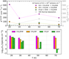 |
Fig. 6 Methanol ice recombination rate as a function of temperature occurring at a selected fluence (top). At all temperatures, reaction R5 (violet circles) occurs faster than reactions R6 (orange squares) and R7 (green diamonds). Hydrogen thermal desorption is indicated by the grey stars and dotted lines. Bottom: logarithm number density of the radicals (X) formed after CH3OH ice photolysis. |
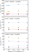 |
Fig. 7 Methanol ice recombination rate as a function of temperature and fluence. Blue pentagons, purple stars, the gold diamond, and the red cross indicate the rates at temperatures of 20, 30, 50 and 70 K, respectively. Panels a, b, and c show the recombination reactions R5–R7, respectively. |
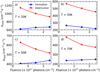 |
Fig. 8 Total formation and destruction rates of CH3OH ice at selected fluences. Except at 30 K, the formation rate (blue line/symbols) increases with fluence while the destruction rate (red line/symbols) decreases. The lack of this trend at 30 K is attributed to the efficient reactive desorption at all fluences (see text). |
4.2 Astrophysical implications
Based on the findings obtained in the previous sections, we assessed the impact of the methanol ice photolysis in the chemical abundances of a molecular cloud subjected to UV radiation field with different strengths. This is worth analysing because in most published astrochemical models, the photolysis of methanol ice is not included.
With ProDiMo, the molecular cloud model is benchmarked against ALCHEMIC and NAUTILUS (Semenov et al. 2010), and it performs 0D time-dependent chemical simulations where AV = 10 mag and Tdust = Tgas are adopted. We used the same temperatures in laboratory experiments. The chemical variations were checked for different physical environments, namely, numerical densities of n = 104 cm−3 and n = 105 cm−3, cosmic ray ionization rates of ζ = 10−16 s−1 and ζ = 10−17 s−1, and a UV radiation strength from χ = 1, which represents inner regions of molecular clouds to χ = 105, which illustrates the high UV field in photon-dominated regions. For completeness, all physical parameters used for the molecular cloud simulations, including the dust grain size (a) and the dust-to-gas mass standard ratio (δ), are given in Table 5. The elemental abundances assumed in these models are shown in Table 6, and the chemical elements, gas-phase species, and additional photolysis reactions are shown in Appendices B and C.1, respectively.
Figure 9 shows the gas-phase methanol abundance with (solid lines) and without (dashed lines) CH3OH ice photodissociation in the chemical simulations of a molecular cloud irradiated by external sources. The abundance observed in the Orion Bar is only for comparison purposes since the molecular cloud model adopted in this paper does not include the physics involved in photo-dominated regions (PDRs). However, the models adopting a temperature of 20 K produce abundances compatible with that astrophysical environment. Qualitatively, the models with and without methanol ice photolysis produce similar abundances for n = 104 cm−3 and, ζ = 10−16 s−1 or ζ = 10−17 s−1 (panels a and b, respectively). On the other hand, when the same H2 ionization rates are adopted for n = 105 cm−3 , great differences are observed (panels c and d).
The quantitative differences of the models with and without methanol ice photolysis are given in Fig. 10 for the gas phase. Panels a and b show that the chemical differences are lower than a factor of five in regions where n = 104 cm−3 and, ζ = 10−16−17 s−1. On the other hand, in denser regions where n = 105 cm−3 (panels c and d), models including methanol ice photolysis result in up to one order of magnitude more gas-phase methanol after 1 × 10⁵ yr. However, the strength of the UV radiation field strength of χ = 104 is required to enhance the methanol gas-phase abundance if the ionization field is ζ = 10−16 s−1. Conversely, assuming a lower H2 ionization rate (ζ = 10−17 s−1), a weaker UV radiation field (χ ≤ 10) is needed to produce such an increment in the gas-phase methanol abundance. The main mechanism that releases methanol into the gas phase in these models is the reactive desorption following reactions R5 and R6 and photodesorption.
This analysis was repeated for temperatures of 30 K, 50 K, and 70 K, where reactive desorption from Minissale et al. (2016) was adopted at 30 K for reasons of consistency with the results in Sect. 3. However, only in the case assuming T = 30 K, n = 105 cm−3, ζ = 10−16 s−1, and χ = 104, is a difference of one order of magnitude in the gas-phase methanol abundance observed for the models including methanol ice photolysis. Overall, this simple analysis indicates that higher densities at 20 and 30 K are needed to observe the effect of the methanol ice photodissociation, whereas at 50 and 70 K, no difference occurs when methanol ice photolysis is taken into account (see Appendix F). A trivial explanation is that at low temperatures, the recombination of dissociated CH3OH is more efficient than at higher temperatures because of the number of available radicals. Consequently, the high number of recombination causes more methanol to be desorbed to the gas phase via reactive desorption. Conversely, in the molecular cloud model at high temperature, reactive desorption does not play a role because of the low number of available radicals for recombination and the lower recombination rates.
Physical parameters used in the chemical simulation of the molecular cloud.
Elements and abundances adopted in the molecular cloud models.
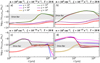 |
Fig. 9 Abundances of gas-phase methanol at different physical conditions and T = 20 K. The solid and dashed lines show the abundances in the models with and without methanol ice photolysis, respectively. The line colours indicate the strength of the UV radiation field. The grey shaded area indicates methanol abundance in the Orion Bar PDR region (Cuadrado et al. 2017) only for comparison purposes with an astrophysical environment. |
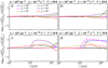 |
Fig. 10 Methanol gas-phase abundance difference in logarithmic scale between the models with and without CH3OH ice photolysis at different physical conditions and T = 20 K. The line colours indicate the strength of the UV radiation field. |
5 Conclusions
The ProDiMo code was used to model the methanol ice photolysis by UV radiation under laboratory conditions. The experiments performed by Öberg et al. (2009a) were used to set up the models introduced in this paper. Different surface chemistry mechanisms and branch ratios were used to run a grid of models and quantify the dependence of the temperature in the ice photolysis. The main results of this work are listed below:
The photodissociation cross sections σphd of the methanol ice derived in this paper agree reasonably well with the experiments. The difference of 10−15% between modelling and the laboratory can be associated with multiple causes, including the cage effect, that is, that the radical diffusion is inhibited by the environment, which leads to a fast CH3OH ice re-formation. Based on the that provides the maximum likelihood between experiment and models, we calculated the temperature-dependent photorates for methanol ice photolysis;
Surface chemistry mechanisms such as diffusion/reaction tunnelling, surface competition, and thermal diffusion are required to reproduce the methanol ice photodissociation observed in the experiments. In addition, the models including reactive desorption from Minissale et al. (2016) fit the experiment at 30 K well, whereas the cases at 20, 50, and 70 K are better fitted when reactive desorption from Garrod et al. (2007) is considered. The reason for this difference is not clear from the analysis introduced in this paper;
The methanol ice BRs calculated by Paardekooper et al. (2016) provide the best agreement with the experimental data when compared with the results adopting other BR estimates from the literature. This indicates that the methanol ice is mostly destroyed by the hydroxymethyl (CH2OH) channel and not by the methyl branch, as is often assumed in the chemical modelling of the ISM;
The abundance of the chemical species formed from the methanol ice photolysis is well replicated in the cases of CH2OH at 20 K and 30 K, CO2 at 50 K, and CH4 at 20 K. A small difference between experiment and model is obtained for the formation of HCO in the ice when a low activation energy (520 K) for the reaction H# + CO# → HCO# is adopted. The model fails to reproduce the other cases addressed in this paper, especially at 70 K. Although this indicates that more accurate surface chemistry approaches are needed, it is also a warning about the accuracy of physicochemical parameters in the reaction network, such as binding energy, radical diffusion rates, and photolysis of other chemical species;
In typical conditions of molecular clouds (high density, low temperature, and standard strength of UV radiation field), CH3OH ice photolysis leads to an enhancement of the gas-phase CH3OH abundance by up to one order of magnitude via chemical desorption.
This study shows that the computational modelling of chemical reactions in the ice under laboratory conditions can be used to shrink the gap between experiments and models to interpret astronomical observations. In particular, the analysis of the current observations with the JWST improves our knowledge of the composition and chemical environment of interstellar ice mantles. Therefore, a quantitative understanding of the processes that govern ice chemistry is crucial. Moreover, this work provides a template for future studies simulating the UV radiation of ice samples.
Acknowledgements
We thank the anonymous referee for providing a throughout constructive report that improved the quality of this paper. This work benefited from support from the European Research Council (ERC) under the European Union's Horizon 2020 research and innovation program through ERC Consolida-tor Grant "S4F" (grant agreement No 646908), and from the ERC "MOLDISK" grant (grant agreement No 101019751). W.R.M.R. acknowledges the São Paulo Research Foundation (grant No 16/23054-7) and the financial support from Leiden Observatory. WRMR also thanks Carlos M. R. Rocha and Ko-Ju Chuang for insightful discussions. P.W. acknowledges funding from the European Union H2020-MSCA-ITN-2019 under Grant Agreement no. 860470 (CHAMELEON). The research of LEK is supported by a research grant (19127) from VILLUM FONDEN.
Appendix A Photorate α
The photodissociation rate is formally defined by
 (A.1)
(A.1)
where σλ is the photodissociation cross section, and Fλ is the flux in units of cm−2 s−2.
In a region shielded by dust, the photodissociation rate is given as
 (A.2)
(A.2)
where α is the photorate of the unshielded region, χ is the FUV strength in the Draine field, γ is the dust attenuation factor, and Av the visual extinction due to dust.
In a region without dust extinction, Av = 0, and from Equations A.1 and A.2, we have
 (A.3)
(A.3)
In a context simulating the laboratory conditions, the flux can be given as a function of the flux lamp, namely,  . To scale this flux with the radiation field from Draine (Draine 1978), we consider the following equation:
 (A.4)
(A.4)
in which the integral boundaries cover the Lyman-α emission at 121 nm. In the denominator, the integrated flux from Draine is equal to 1.9921 × 108 cm−2 s−1 (see Equation 2).
Isolating the photorate term in Equation A.3, we have that
 (A.5)
(A.5)
The ratio of the two intregrals in Equation A.5 is equal to the average photodissociation cross section ( ) and can be rewritten as
 (A.6)
(A.6)
Appendix B Chemical elements in the network
The chemical elements, gas- and solid-phase chemical species adopted used in this study are shown in Table B.1.
Gas and solid species in the network.
Appendix C Ice photodissociation rates
The photodissociation rates of the molecules in ices adopted in this work are shown in Table C.1.
Ice photodissociation rates (α) and the dust attenuation factor (γ) for other photodissociation reactions used in Equation A.2.
Appendix D Bimolecular surface reactions rates and binding energies
The bimolecular surface reaction rates used in this paper are shown in Table D.1, and the binding energies are shown in Table D.2.
List of bimolecular surface reactions used in this paper and their respective energies barrier (ΔΕ). See Equation 9.
List of binding energies.
Appendix E Gallery of fits at 20 K, 30 K, 50 K, and 70 K
The grid of photodissociation models at four temperatures and adopting different surface chemistry parameters is shown in this appendix. Figures E.1-E.5 show the fits at 20 K for models 3–7. Figures E.6-E.10 show the fits at 30 K for models 3–7. In these fits, only the models adopting reactive desorption from Minissale et al. (2016) fit the experimental data well. Figures E.11-E.17 show the fits at 50 K for models 1–7. Figures E.18-E.24 show the fits at 70 K for models 1–7.
 |
Fig. E.1 Grid of methanol ice photodissociation models at 20 K assuming different photodissociation cross sections and BRs. The model 3 in Table 2 is adopted in these plots. |
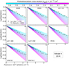 |
Fig. E.2 Same as Figure E.1, but adopting model 4. |
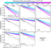 |
Fig. E.3 Same as Figure E.1, but adopting model 5. |
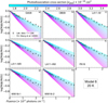 |
Fig. E.4 Same as Figure E.1, but adopting model 6. |
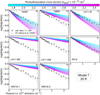 |
Fig. E.5 Same as Figure E.1, but adopting model 7. |
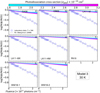 |
Fig. E.6 Grid of methanol ice photodissociation models at 30 K assuming different photodissociation cross sections and BRs. Model 3 in Table 2 is adopted in these plots. |
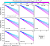 |
Fig. E.7 Same as Figure E.6, but adopting model 4. |
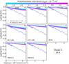 |
Fig. E.8 Same as Figure E.6, but adopting model 5. |
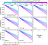 |
Fig. E.9 Same as Figure E.6, but adopting model 6. |
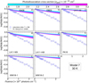 |
Fig. E.10 Same as Figure E.6, but adopting model 7. |
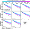 |
Fig. E.11 Grid of methanol ice photodissociation models at 50 K assuming different photodissociation cross sections and BRs. Model 1 in Table 2 is adopted in these plots. |
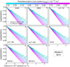 |
Fig. E.12 Same as Figure E.11, but adopting model 2. |
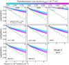 |
Fig. E.13 Same as Figure E.11, but adopting model 3. |
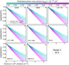 |
Fig. E.14 Same as Figure E.11, but adopting model 4. |
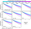 |
Fig. E.15 Same as Figure E.11, but adopting model 5. |
 |
Fig. E.16 Same as Figure E.11, but adopting model 6. |
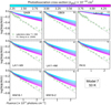 |
Fig. E.17 Same as Figure E.11, but adopting model 7. |
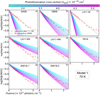 |
Fig. E.18 Grid of methanol ice photodissociation models at 70 K assuming different photodissociation cross sections and BRs. Model 1 in Table is adopted in these plots. |
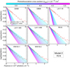 |
Fig. E.19 Same as Figure E.18, but adopting model 2. |
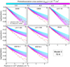 |
Fig. E.20 Same as Figure E.11, but adopting model 3. |
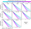 |
Fig. E.21 Same as Figure E.11, but adopting model 4. |
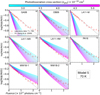 |
Fig. E.22 Same as Figure E.11, but adopting model 5. |
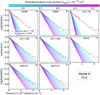 |
Fig. E.23 Same as Figure E.11, but adopting model 6. |
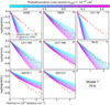 |
Fig. E.24 Same as Figure E.11, but adopting model 7. |
Appendix F CH3OH gas-phase abundances at 30 K, 50 K, and 70 K in the molecular cloud model
The methanol gas-phase abundances in the molecular cloud model at three temperatures and adopting different numerical densities and H2 ionization rates are shown in Figures F.1–F.3. In these cases, the difference between models including or excluding methanol ice photolysis is negligible. Additionally, the abundances mostly deviate from the observations toward the Orion Bar.
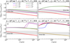 |
Fig. F.1 Abundances of gas-phase methanol at different physical conditions and T = 30 K. The solid and dashed lines show the abundances in the models with and without methanol ice photolysis, respectively. The line colours indicate the strength of the UV radiation field. The grey shaded area indicates the methanol abundance in the Orion Bar PDR (Cuadrado et al. 2017) only for comparison purposes with an astrophysical environment. |
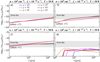 |
Fig. F.2 Same as Figure F.1, but for Τ = 50 Κ. |
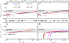 |
Fig. F.3 Same as Figure F.1, but for Τ = 70 Κ. |
References
- Acharyya, K., Fuchs, G. W., Fraser, H. J., van Dishoeck, E. F., & Linnartz, H. 2007, A&A, 466, 1005 [NASA ADS] [CrossRef] [EDP Sciences] [Google Scholar]
- Aikawa, Y., Miyama, S. M., Nakano, T., & Umebayashi, T. 1996, ApJ, 467, 684 [NASA ADS] [CrossRef] [Google Scholar]
- Aikawa, Y., Wakelam, V., Garrod, R. T., & Herbst, E. 2008, ApJ, 674, 984 [NASA ADS] [CrossRef] [Google Scholar]
- Ashfold, M. N. R., King, G. A., Murdock, D., et al. 2010, Phys. Chem. Chem. Phys. (Incorp. Faraday Trans.), 12, 1218 [NASA ADS] [CrossRef] [Google Scholar]
- Awad, Z., Chigai, T., Kimura, Y., Shalabiea, O. M., & Yamamoto, T. 2005, ApJ, 626, 262 [NASA ADS] [CrossRef] [Google Scholar]
- Balsiger, H., Altwegg, K., Bochsler, P., et al. 2007, Space Sci. Rev., 128, 745 [NASA ADS] [CrossRef] [Google Scholar]
- Bell, R. P. 1980, The Tunnel Effect in Chemistry (New York: Springer, 2013) [Google Scholar]
- Bell, R. P., & Le Roy, R. J. 1982, Phys. Today, 35, 85 [NASA ADS] [CrossRef] [Google Scholar]
- Bertin, M., Romanzin, C., Doronin, M., et al. 2016, ApJ, 817, L12 [NASA ADS] [CrossRef] [Google Scholar]
- Bixon, M., & Jortner, J. 1968, J. Chem. Phys., 48, 715 [NASA ADS] [CrossRef] [Google Scholar]
- Boogert, A. C. A., Huard, T. L., Cook, A. M., et al. 2011, ApJ, 729, 92 [NASA ADS] [CrossRef] [Google Scholar]
- Bovolenta, G. M., Vogt-Geisse, S., Bovino, S., & Grassi, T. 2022, ApJS, 262, 17 [NASA ADS] [CrossRef] [Google Scholar]
- Brown, W. A., & Bolina, A. S. 2007, MNRAS, 374, 1006 [NASA ADS] [CrossRef] [Google Scholar]
- Brown, W. L., Augustyniak, W. M., Marcantonio, K. J., et al. 1984, Nucl. Instrum. Methods Phys. Res. B, 1, 307 [NASA ADS] [CrossRef] [Google Scholar]
- Calmonte, U., Altwegg, K., Balsiger, H., et al. 2016, MNRAS, 462, S253 [NASA ADS] [CrossRef] [Google Scholar]
- Carvalho, G. A., Pilling, S., & Galvão, B. R. L. 2022, MNRAS, 515, 3760 [NASA ADS] [CrossRef] [Google Scholar]
- Cazaux, S., & Tielens, A. G. G. M. 2002, ApJ, 575, L29 [NASA ADS] [CrossRef] [Google Scholar]
- Chaabouni, H., Minissale, M., Manicò, G., et al. 2012, J. Chem. Phys., 137, 234706 [NASA ADS] [CrossRef] [Google Scholar]
- Chiar, J. E., Tielens, A. G. G. M., Whittet, D. C. B., et al. 2000, ApJ, 537, 749 [NASA ADS] [CrossRef] [Google Scholar]
- Chu, L. E. U., Hodapp, K., & Boogert, A. 2020, ApJ, 904, 86 [NASA ADS] [CrossRef] [Google Scholar]
- Clark, P. C., Glover, S. C. O., Klessen, R. S., & Bonnell, I. A. 2012, MNRAS, 424, 2599 [CrossRef] [Google Scholar]
- Collings, M. P., Anderson, M. A., Chen, R., et al. 2004, MNRAS, 354, 1133 [NASA ADS] [CrossRef] [Google Scholar]
- Congiu, E., Minissale, M., Baouche, S., et al. 2014, Faraday Discuss., 168, 151 [NASA ADS] [CrossRef] [Google Scholar]
- Cuadrado, S., Goicoechea, J. R., Cernicharo, J., et al. 2017, A&A, 603, A124 [NASA ADS] [CrossRef] [EDP Sciences] [Google Scholar]
- Cuppen, H. M., Walsh, C., Lamberts, T., et al. 2017, Space Sci. Rev., 212, 1 [Google Scholar]
- Dartois, E., Chabot, M., Id Barkach, T., et al. 2018, A&A, 618, A173 [NASA ADS] [CrossRef] [EDP Sciences] [Google Scholar]
- Draine, B. T. 1978, ApJS, 36, 595 [Google Scholar]
- Draine, B. T., & Bertoldi, F. 1996, ApJ, 468, 269 [Google Scholar]
- Drozdovskaya, M. N., Schroeder I. I. R. H. G., Rubin, M., et al. 2021, MNRAS, 500, 4901 [Google Scholar]
- Dulieu, F., Congiu, E., Noble, J., et al. 2013, Sci. Rep., 3, 1338 [Google Scholar]
- Edridge, J. L. 2010, PhD thesis, University of London, University College London (UK) [Google Scholar]
- Esplugues, G. B., Cazaux, S., Meijerink, R., Spaans, M., & Caselli, P. 2016, A&A, 591, A52 [NASA ADS] [CrossRef] [EDP Sciences] [Google Scholar]
- Fahr, A., & Laufer, A. H. 1995, J. Phys. Chem., 99, 262 [Google Scholar]
- Fayolle, E. C., Bertin, M., Romanzin, C., et al. 2011, ApJ, 739, L36 [Google Scholar]
- Franck, J., & Rabinowitsch, E. 1934, Trans. Faraday Soc., 30, 120 [Google Scholar]
- Fuchs, G. W., Cuppen, H. M., Ioppolo, S., et al. 2009, A&A, 505, 629 [NASA ADS] [CrossRef] [EDP Sciences] [Google Scholar]
- Garrod, R. T., & Herbst, E. 2006, A&A, 457, 927 [NASA ADS] [CrossRef] [EDP Sciences] [Google Scholar]
- Garrod, R. T., & Pauly, T. 2011, ApJ, 735, 15 [Google Scholar]
- Garrod, R. T., Wakelam, V., & Herbst, E. 2007, A&A, 467, 1103 [NASA ADS] [CrossRef] [EDP Sciences] [Google Scholar]
- Garrod, R. T., Widicus Weaver, S. L., & Herbst, E. 2008, ApJ, 682, 283 [Google Scholar]
- Goto, M., Vasyunin, A. I., Giuliano, B. M., et al. 2021, A&A, 651, A53 [NASA ADS] [CrossRef] [EDP Sciences] [Google Scholar]
- Goumans, T. P. M., Uppal, M. A., & Brown, W. A. 2008, MNRAS, 384, 1158 [NASA ADS] [CrossRef] [Google Scholar]
- Grassi, T., Bovino, S., Caselli, P., et al. 2020, A&A, 643, A155 [EDP Sciences] [Google Scholar]
- Grundy, W. M., Bird, M. K., Britt, D. T., et al. 2020, Science, 367, aay3705 [NASA ADS] [CrossRef] [Google Scholar]
- Hagege, J., Roberge, P. C., & Vermeil, C. 1968, Trans. Faraday Soc., 64, 3288 [Google Scholar]
- Hasegawa, T. I., & Herbst, E. 1993, MNRAS, 263, 589 [Google Scholar]
- Herbst, E., & Millar, T. J. 2008, Low Temperatures and Cold Molecules, ed. I. W. M. Smith (London: Imperial College Press), 1 [Google Scholar]
- Herrero, V. J., Gálvez, Ó., Maté, B., & Escribano, R. 2010, Phys. Chem. Chem. Phys. (Incorp. Faraday Trans.), 12, 3164 [NASA ADS] [CrossRef] [Google Scholar]
- Holbrook, K. A. K. A., Pilling, M. J., & Robertson, S. H. 1996, Unimolecular Reactions, eds. K. A. Holbrook, M. J. Pilling, & S. H. Robertson, 2nd edn. (Chichester: John Wiley & Sons) [Google Scholar]
- Ioppolo, S., Cuppen, H. M., Romanzin, C., van Dishoeck, E. F., & Linnartz, H. 2008, ApJ, 686, 1474 [NASA ADS] [CrossRef] [Google Scholar]
- Ioppolo, S., Fedoseev, G., Chuang, K. J., et al. 2021, Nat. Astron., 5, 197 [NASA ADS] [CrossRef] [Google Scholar]
- Jiménez-Escobar, A., Chen, Y. J., Ciaravella, A., et al. 2016, ApJ, 820, 25 [CrossRef] [Google Scholar]
- Jochims, H. W., Ruhl, E., Baumgartel, H., Tobita, S., & Leach, S. 1994, ApJ, 420, 307 [NASA ADS] [CrossRef] [Google Scholar]
- Kamp, I., Tilling, I., Woitke, P., Thi, W. F., & Hogerheijde, M. 2010, A&A, 510, A18 [NASA ADS] [CrossRef] [EDP Sciences] [Google Scholar]
- Kim, J., Lee, J.-E., Jeong, W.-S., et al. 2022, ApJ, 935, 137 [NASA ADS] [CrossRef] [Google Scholar]
- Kristensen, L. E., van Dishoeck, E. F., van Kempen, T. A., et al. 2010, A&A, 516, A57 [NASA ADS] [CrossRef] [EDP Sciences] [Google Scholar]
- Kroes, G. J., & Andersson, S. 2005, IAU Symposium, 231, 427 [NASA ADS] [Google Scholar]
- Kuwahata, K., Hama, T., Kouchi, A., & Watanabe, N. 2015, Phys. Rev. Lett., 115, 133201 [NASA ADS] [CrossRef] [Google Scholar]
- Laas, J. C., Garrod, R. T., Herbst, E., & Widicus Weaver, S. L. 2011, ApJ, 728, 71 [Google Scholar]
- Laffon, C., Lasne, J., Bournel, F., et al. 2010, Phys. Chem. Chem. Phys. (Incorp. Faraday Trans.), 12, 10865 [NASA ADS] [CrossRef] [Google Scholar]
- Lamberts, T., Cuppen, H. M., Fedoseev, G., et al. 2014, A&A, 570, A57 [NASA ADS] [CrossRef] [EDP Sciences] [Google Scholar]
- Lamberts, T., Samanta, P. K., Köhn, A., & Kästner, J. 2016, Phys. Chem. Chem. Phys. (Incorp. Faraday Trans.), 18, 33021 [NASA ADS] [CrossRef] [Google Scholar]
- Lara, L. M., Lellouch, E., González, M., Moreno, R., & Rengel, M. 2014, A&A, 566, A143 [NASA ADS] [CrossRef] [EDP Sciences] [Google Scholar]
- Lavvas, P. P., Coustenis, A., & Vardavas, I. M. 2008, Planet. Space Sci., 56, 27 [NASA ADS] [CrossRef] [Google Scholar]
- Le Roy, L., Altwegg, K., Balsiger, H., et al. 2015, A&A, 583, A1 [NASA ADS] [CrossRef] [EDP Sciences] [Google Scholar]
- Leger, A., D’Hendecourt, L., Boissel, P., & Desert, F. X. 1989, A&A, 213, 351 [NASA ADS] [Google Scholar]
- Li, Q. S., Zhang, Y., & Zhang, S. 2004, J. Chem. Phys., 121, 9474 [NASA ADS] [CrossRef] [Google Scholar]
- Ligterink, N. F. W., Paardekooper, D. M., Chuang, K. J., et al. 2015, A&A, 584, A56 [NASA ADS] [CrossRef] [EDP Sciences] [Google Scholar]
- McClure, M. K., Rocha, W. R. M., Pontoppidan, K. M., et al. 2023, Nat. Astron., 1747, 946 [Google Scholar]
- Meinert, C., Myrgorodska, I., de Marcellus, P., et al. 2016, Science, 352, 208 [NASA ADS] [CrossRef] [Google Scholar]
- Minissale, M., Loison, J. C., Baouche, S., et al. 2015, A&A, 577, A2 [NASA ADS] [CrossRef] [EDP Sciences] [Google Scholar]
- Minissale, M., Dulieu, F., Cazaux, S., & Hocuk, S. 2016, A&A, 585, A24 [NASA ADS] [CrossRef] [EDP Sciences] [Google Scholar]
- Minissale, M., Aikawa, Y., Bergin, E., et al. 2022, ACS Earth Space Chem., 6, 597 [NASA ADS] [CrossRef] [Google Scholar]
- Mullikin, E., Anderson, H., O’Hern, N., et al. 2021, ApJ, 910, 72 [NASA ADS] [CrossRef] [Google Scholar]
- Nuevo, M., Cooper, G., & Sandford, S. A. 2018, Nat. Commun., 9, 5276 [NASA ADS] [CrossRef] [Google Scholar]
- Oba, Y., Watanabe, N., Hama, T., et al. 2012, ApJ, 749, 67 [Google Scholar]
- Öberg, K. I. 2016, Chem. Rev., 116, 9631 [Google Scholar]
- Öberg, K. I., Garrod, R. T., van Dishoeck, E. F., & Linnartz, H. 2009a, A&A, 504, 891 [NASA ADS] [CrossRef] [EDP Sciences] [Google Scholar]
- Öberg, K. I., van Dishoeck, E. F., & Linnartz, H. 2009b, A&A, 496, 281 [NASA ADS] [CrossRef] [EDP Sciences] [Google Scholar]
- Öberg, K. I., Boogert, A. C. A., Pontoppidan, K. M., et al. 2011, ApJ, 740, 109 [Google Scholar]
- Opansky, B. J., & Leone, S. R. 1996, J. Phys. Chem., 100, 19904 [CrossRef] [Google Scholar]
- Paardekooper, D. M., Bossa, J. B., & Linnartz, H. 2016, A&A, 592, A67 [NASA ADS] [CrossRef] [EDP Sciences] [Google Scholar]
- Perotti, G., Rocha, W. R. M., Jørgensen, J. K., et al. 2020, A&A, 643, A48 [EDP Sciences] [Google Scholar]
- Perotti, G., Jørgensen, J. K., Fraser, H. J., et al. 2021, A&A, 650, A168 [NASA ADS] [CrossRef] [EDP Sciences] [Google Scholar]
- Pilling, S., Carvalho, G. A., & Rocha, W. R. M. 2022, ApJ, 925, 147 [NASA ADS] [CrossRef] [Google Scholar]
- Pilling, S., Rocha, W. R. M., Carvalho, G. A., & de Abreu, H. A. 2023, ASR, submitted [Google Scholar]
- Pontoppidan, K. M., van Dishoeck, E. F., & Dartois, E. 2004, A&A, 426, 925 [NASA ADS] [CrossRef] [EDP Sciences] [Google Scholar]
- Prasad, S. S., & Tarafdar, S. P. 1983, ApJ, 267, 603 [Google Scholar]
- Qasim, D., Chuang, K. J., Fedoseev, G., et al. 2018, A&A, 612, A83 [NASA ADS] [CrossRef] [EDP Sciences] [Google Scholar]
- Raut, U., & Baragiola, R. A. 2011, ApJ, 737, L14 [NASA ADS] [CrossRef] [Google Scholar]
- Rimola, A., Taquet, V., Ugliengo, P., Balucani, N., & Ceccarelli, C. 2014, A&A, 572, A70 [NASA ADS] [CrossRef] [EDP Sciences] [Google Scholar]
- Roncero, O., Zanchet, A., & Aguado, A. 2018, Phys. Chem. Chem. Phys. (Incorp. Faraday Trans.), 20, 25951 [NASA ADS] [CrossRef] [Google Scholar]
- Ruaud, M., Loison, J. C., Hickson, K. M., et al. 2015, MNRAS, 447, 4004 [Google Scholar]
- Ruffle, D. P., & Herbst, E. 2000, MNRAS, 319, 837 [Google Scholar]
- Santos, J. C., Chuang, K.-J., Lamberts, T., et al. 2022, ApJ, 931, L33 [NASA ADS] [CrossRef] [Google Scholar]
- Schutte, W. A., Tielens, A. G. G., & Sandford, S. A. 1991, ApJ, 382, 523 [NASA ADS] [CrossRef] [Google Scholar]
- Semenov, D., Hersant, F., Wakelam, V., et al. 2010, A&A, 522, A42 [NASA ADS] [CrossRef] [EDP Sciences] [Google Scholar]
- Shen, C. J., Greenberg, J. M., Schutte, W. A., & van Dishoeck, E. F. 2004, A&A, 415, 203 [NASA ADS] [CrossRef] [EDP Sciences] [Google Scholar]
- Shimonishi, T., Nakatani, N., Furuya, K., & Hama, T. 2018, ApJ, 855, 27 [Google Scholar]
- Shingledecker, C. N., Vasyunin, A., Herbst, E., & Caselli, P. 2019, ApJ, 876, 140 [Google Scholar]
- Shingledecker, C. N., Lamberts, T., Laas, J. C., et al. 2020, ApJ, 888, 52 [Google Scholar]
- Skouteris, D., Balucani, N., Ceccarelli, C., et al. 2018, ApJ, 854, 135 [NASA ADS] [CrossRef] [Google Scholar]
- Thi, W. F., Woitke, P., & Kamp, I. 2011, MNRAS, 412, 711 [Google Scholar]
- Thi, W. F., Hocuk, S., Kamp, I., et al. 2020a, A&A, 634, A42 [NASA ADS] [CrossRef] [EDP Sciences] [Google Scholar]
- Thi, W. F., Hocuk, S., Kamp, I., et al. 2020b, A&A, 635, A16 [NASA ADS] [CrossRef] [EDP Sciences] [Google Scholar]
- Tielens, A. G. G. M., & Hagen, W. 1982, A&A, 114, 245 [Google Scholar]
- Tramer, A., & Voltz, R. 1979, in Excited States, 4, Time-Resolved Studies of Excited Molecules, ed. E. C. Lim (Elsevier), 281 [Google Scholar]
- van Dishoeck, E. F., & Visser, R. 2011, ArXiv e-prints [arXiv:1106.3917] [Google Scholar]
- Vasyunin, A. I., & Herbst, E. 2013, ApJ, 769, 34 [Google Scholar]
- Vasyunin, A. I., Caselli, P., Dulieu, F., & Jiménez-Serra, I. 2017, ApJ, 842, 33 [Google Scholar]
- Villadsen, T., Ligterink, N. F. W., & Andersen, M. 2022, A&A, 666, A45 [NASA ADS] [CrossRef] [EDP Sciences] [Google Scholar]
- Wakelam, V., Loison, J. C., Mereau, R., & Ruaud, M. 2017, Mol. Astrophys., 6, 22 [NASA ADS] [CrossRef] [Google Scholar]
- Watanabe, N., & Kouchi, A. 2002, ApJ, 571, L173 [Google Scholar]
- Weaver, S. W., Powers, C. R., McCabe, M. N., & Zinga, S. 2018, IAU Symp., 332, 305 [NASA ADS] [Google Scholar]
- Westley, M. S., Baragiola, R. A., Johnson, R. E., & Baratta, G. A. 1995, Planet. Space Sci., 43, 1311 [NASA ADS] [CrossRef] [Google Scholar]
- Woitke, P., Kamp, I., & Thi, W. F. 2009, A&A, 501, 383 [NASA ADS] [CrossRef] [EDP Sciences] [Google Scholar]
- Yang, Y.-L., Green, J. D., Pontoppidan, K. M., et al. 2022, ApJ, 941, L13 [NASA ADS] [CrossRef] [Google Scholar]
- Yocum, K. M., Milam, S. N., Gerakines, P. A., & Widicus Weaver, S. L. 2021, ApJ, 913, 61 [NASA ADS] [CrossRef] [Google Scholar]
All Tables
Methanol ice photodissociation pathways and unshielded photorates () taken from the best models.
Ice photodissociation rates (α) and the dust attenuation factor (γ) for other photodissociation reactions used in Equation A.2.
List of bimolecular surface reactions used in this paper and their respective energies barrier (ΔΕ). See Equation 9.
All Figures
|
Fig. 1 Comparison between the UV flux distribution of the interstellar radiation field (χ) from Draine (1978) and from the lamps used in the laboratory for ice photochemistry. |
| In the text | |
|
Fig. 2 Grid of methanol ice photodissociation in models 1 and 2 at 20 K (left panel) and at 30 K (right panel). The models assume different photodissociation cross sections and BRs (see Table 1). These models assume surface competition, diffusion, reaction tunnelling, and thermal diffusion. In addition, models 1 and 2 adopt the reactive desorption formalism from Garrod et al. (2007) and Minissale et al. (2016), respectively. |
| In the text | |
|
Fig. 3 Accuracy of the CH3OH ice photodissociation fit for models 1–7. Higher bars indicate the best models. When no bars are shown, the MLE values are lower than the y-axis threshold. The hatched and solid bars indicate the models assuming the reactive desorption mechanism by Minissale et al. (2016) and Garrod et al. (2007), respectively. |
| In the text | |
|
Fig. 4 Natural logarithm of the normalized CH3OH ice column density as a function of the UV fluence at 20, 30, 50, and 70 K in panels a–d, respectively. The symbols show the laboratory data from Öberg et al. (2009a), and the lines indicate the models that match the experiments best. |
| In the text | |
|
Fig. 5 Formation curves of selected daughter species (CH2OH, CO, CO2, CH4, HCO, and H2CO) due to CH3OH photolysis over fluence with respect to the initial methanol ice column density at four temperatures. The symbols are the experimental measurements, and the solid lines are the results of ProDiMo simulations of the best photodissociation models (see Fig. 4). |
| In the text | |
|
Fig. 6 Methanol ice recombination rate as a function of temperature occurring at a selected fluence (top). At all temperatures, reaction R5 (violet circles) occurs faster than reactions R6 (orange squares) and R7 (green diamonds). Hydrogen thermal desorption is indicated by the grey stars and dotted lines. Bottom: logarithm number density of the radicals (X) formed after CH3OH ice photolysis. |
| In the text | |
|
Fig. 7 Methanol ice recombination rate as a function of temperature and fluence. Blue pentagons, purple stars, the gold diamond, and the red cross indicate the rates at temperatures of 20, 30, 50 and 70 K, respectively. Panels a, b, and c show the recombination reactions R5–R7, respectively. |
| In the text | |
|
Fig. 8 Total formation and destruction rates of CH3OH ice at selected fluences. Except at 30 K, the formation rate (blue line/symbols) increases with fluence while the destruction rate (red line/symbols) decreases. The lack of this trend at 30 K is attributed to the efficient reactive desorption at all fluences (see text). |
| In the text | |
|
Fig. 9 Abundances of gas-phase methanol at different physical conditions and T = 20 K. The solid and dashed lines show the abundances in the models with and without methanol ice photolysis, respectively. The line colours indicate the strength of the UV radiation field. The grey shaded area indicates methanol abundance in the Orion Bar PDR region (Cuadrado et al. 2017) only for comparison purposes with an astrophysical environment. |
| In the text | |
|
Fig. 10 Methanol gas-phase abundance difference in logarithmic scale between the models with and without CH3OH ice photolysis at different physical conditions and T = 20 K. The line colours indicate the strength of the UV radiation field. |
| In the text | |
|
Fig. E.1 Grid of methanol ice photodissociation models at 20 K assuming different photodissociation cross sections and BRs. The model 3 in Table 2 is adopted in these plots. |
| In the text | |
|
Fig. E.2 Same as Figure E.1, but adopting model 4. |
| In the text | |
|
Fig. E.3 Same as Figure E.1, but adopting model 5. |
| In the text | |
|
Fig. E.4 Same as Figure E.1, but adopting model 6. |
| In the text | |
|
Fig. E.5 Same as Figure E.1, but adopting model 7. |
| In the text | |
|
Fig. E.6 Grid of methanol ice photodissociation models at 30 K assuming different photodissociation cross sections and BRs. Model 3 in Table 2 is adopted in these plots. |
| In the text | |
|
Fig. E.7 Same as Figure E.6, but adopting model 4. |
| In the text | |
|
Fig. E.8 Same as Figure E.6, but adopting model 5. |
| In the text | |
|
Fig. E.9 Same as Figure E.6, but adopting model 6. |
| In the text | |
|
Fig. E.10 Same as Figure E.6, but adopting model 7. |
| In the text | |
|
Fig. E.11 Grid of methanol ice photodissociation models at 50 K assuming different photodissociation cross sections and BRs. Model 1 in Table 2 is adopted in these plots. |
| In the text | |
|
Fig. E.12 Same as Figure E.11, but adopting model 2. |
| In the text | |
|
Fig. E.13 Same as Figure E.11, but adopting model 3. |
| In the text | |
|
Fig. E.14 Same as Figure E.11, but adopting model 4. |
| In the text | |
|
Fig. E.15 Same as Figure E.11, but adopting model 5. |
| In the text | |
|
Fig. E.16 Same as Figure E.11, but adopting model 6. |
| In the text | |
|
Fig. E.17 Same as Figure E.11, but adopting model 7. |
| In the text | |
|
Fig. E.18 Grid of methanol ice photodissociation models at 70 K assuming different photodissociation cross sections and BRs. Model 1 in Table is adopted in these plots. |
| In the text | |
|
Fig. E.19 Same as Figure E.18, but adopting model 2. |
| In the text | |
|
Fig. E.20 Same as Figure E.11, but adopting model 3. |
| In the text | |
|
Fig. E.21 Same as Figure E.11, but adopting model 4. |
| In the text | |
|
Fig. E.22 Same as Figure E.11, but adopting model 5. |
| In the text | |
|
Fig. E.23 Same as Figure E.11, but adopting model 6. |
| In the text | |
|
Fig. E.24 Same as Figure E.11, but adopting model 7. |
| In the text | |
|
Fig. F.1 Abundances of gas-phase methanol at different physical conditions and T = 30 K. The solid and dashed lines show the abundances in the models with and without methanol ice photolysis, respectively. The line colours indicate the strength of the UV radiation field. The grey shaded area indicates the methanol abundance in the Orion Bar PDR (Cuadrado et al. 2017) only for comparison purposes with an astrophysical environment. |
| In the text | |
|
Fig. F.2 Same as Figure F.1, but for Τ = 50 Κ. |
| In the text | |
|
Fig. F.3 Same as Figure F.1, but for Τ = 70 Κ. |
| In the text | |
Current usage metrics show cumulative count of Article Views (full-text article views including HTML views, PDF and ePub downloads, according to the available data) and Abstracts Views on Vision4Press platform.
Data correspond to usage on the plateform after 2015. The current usage metrics is available 48-96 hours after online publication and is updated daily on week days.
Initial download of the metrics may take a while.