| Issue |
A&A
Volume 672, April 2023
|
|
|---|---|---|
| Article Number | A137 | |
| Number of page(s) | 20 | |
| Section | Extragalactic astronomy | |
| DOI | https://doi.org/10.1051/0004-6361/202245168 | |
| Published online | 12 April 2023 | |
The miniJPAS survey: AGN and host galaxy coevolution of X-ray-selected sources⋆
1
Dipartimento di Fisica e Astronomia “Augusto Righi”, Università di Bologna, Via Gobetti 93/2, 40129 Bologna, Italy
e-mail: This email address is being protected from spambots. You need JavaScript enabled to view it.
2
INAF – Osservatorio di Astrofisica e Scienza dello Spazio di Bologna, Via Gobetti 93/3, 40129 Bologna, Italy
3
Donostia International Physics Center (DIPC), Manuel Lardizabal Ibilbidea, 4, Donostia-San, Sebastián, Spain
4
IKERBASQUE, Basque Foundation for Science, 48013 Bilbao, Spain
5
School of Physics and Astronomy, University of Southampton, Highfield, Southampton SO17 1BJ, UK
6
Institute for Astronomy & Astrophysics, National Observatory of Athens, V. Paulou & I. Metaxa, Athens 11532, Greece
7
Centre for Extragalactic Astronomy, Department of Physics, Durham University, Durham DH1 3LE, UK
8
Universitäts-Sternwarte, Fakultät für Physik, Ludwig-Maximilians-Universität München, Scheinerstr.1, 81679 München, Germany
9
Max-Planck-Institut für Astrophysik, Karl-Schwarzschild-Straße 1, 85741 Garching, Germany
10
SISSA, Via Bonomea 265, 34136 Trieste, Italy
11
Instituto de Astrofísica de Canarias, Calle Vía Láctea, s/n, 38205 La Laguna, Tenerife, Spain
12
Departamento de Astrofísica, Universidad de La Laguna, 38206 La Laguna, Tenerife, Spain
13
Exzellenzcluster ORIGINS, Boltzmannstr. 2, 85748 Garching, Germany
14
Institut de Física d’Altes Energies, The Barcelona Institute of Science and Technology, Campus UAB, 08193 Bellaterra, Barcelona, Spain
15
Universidade de São Paulo, Instituto de Astronomia, Geofísica e Ciências Atmosféricas, Rua do Matão, 1226, 05508-090 São Paulo, SP, Brazil
16
Centro de Estudios de Física del Cosmos de Aragón (CEFCA), Unidad Asociada al CSIC, Plaza San Juan, 1, 44001 Teruel, Spain
17
Instituto de Astrofísica de Andalucía (IAA-CSIC), Glorieta de la Astronomía s/n, 18008 Granada, Spain
18
Astronomy and Astrophysics Research and Development Department, Entoto Observatory and Research Center (EORC), Space Science and Geospatial Institute (SSGI), PO Box 33679 Addis Ababa, Ethiopia
19
Physics Department, Faculty of Science, Mbarara University of Science and Technology (MUST), PO Box 1410 Mbarara, Uganda
20
College of Astronomy and Space Sciences, University of the Chinese Academy of Sciences, Beijing 100049, PR China
21
Sydney Institute for Astronomy, School of Physics A28, The University of Sydney, Sydney, NSW 2006, Australia
22
INAF – Osservatorio Astrofisico di Torino, Strada Osservatorio 20, 10025 Pino Torinese, Italy
23
Departamento de Física Matemática, Instituto de Física, Universidade de São Paulo, Rua do Matão, 1371, CEP 05508-090 São Paulo, Brazil
24
Departamento de Astronomia, Instituto de Física, Universidade Federal do Rio Grande do Sul (UFRGS), Av. Bento Gonçalves, 9500 Porto Alegre, RS, Brazil
25
CAS Key Laboratory for Research in Galaxies and Cosmology, Shanghai Astronomical Observatory, CAS, Shanghai 200030, PR China
26
Observatório Nacional, Rua General José Cristino, 77, São Cristóvão, 20921-400 Rio de Janeiro, RJ, Brazil
27
Instituto de Física, Universidade Federal da Bahia, 40210-340 Salvador, BA, Brazil
28
Instruments4, 4121 Pembury Place, La Canada Flintridge, CA 91011, USA
Received:
7
October
2022
Accepted:
31
January
2023
Abstract
Studies indicate strong evidence of a scaling relation in the local Universe between the supermassive black hole mass (MBH) and the stellar mass of their host galaxies (M⋆). They even show similar histories across cosmic times of their differential terms: the star formation rate (SFR) and black hole accretion rate (BHAR). However, a clear picture of this coevolution is far from being understood. We selected an X-ray sample of active galactic nuclei (AGN) up to z = 2.5 in the miniJPAS footprint. Their X-ray to infrared spectral energy distributions (SEDs) have been modeled with the CIGALE code, constraining the emission to 68 bands, from which 54 are the narrow filters from the miniJPAS survey. For a final sample of 308 galaxies, we derived their physical properties, such as their M⋆, SFR, star formation history (SFH), and the luminosity produced by the accretion process of the central BH (LAGN). For a subsample of 113 sources, we also fit their optical spectra to obtain the gas velocity dispersion from the broad emission lines and estimated the MBH. We calculated the BHAR in physical units depending on two radiative efficiency regimes. We find that the Eddington ratios (λEdd) and its popular proxy (LX/M⋆) have a difference of 0.6 dex, on average, and a KS test indicates that they come from different distributions. Our sources exhibit a considerable scatter on the MBH − M⋆ scaling relation, which can explain the difference between λEdd and its proxy. We also modeled three evolution scenarios for each source to recover the integral properties at z = 0. Using the SFR and BHAR, we show a notable diminution in the scattering between MBH − M⋆. For the last scenario, we considered the SFH and a simple energy budget for the AGN accretion, and we retrieved a relation similar to the calibrations known for the local Universe. Our study covers ∼1 deg2 in the sky and is sensitive to biases in luminosity. Nevertheless, we show that, for bright sources, the link between the differential values (SFR and BHAR) and their decoupling based on an energy limit is the key that leads to the local MBH − M⋆ scaling relation. In the future, we plan to extend this methodology to a thousand degrees of the sky using JPAS with an X-ray selection from eROSITA, to obtain an unbiased distribution of BHAR and Eddington ratios.
Key words: galaxies: evolution / galaxies: active / galaxies: nuclei / galaxies: photometry / quasars: supermassive black holes
Full Tables 2 and 6 are only available at the CDS via anonymous ftp to cdsarc.cds.unistra.fr (130.79.128.5) or via https://cdsarc.cds.unistra.fr/viz-bin/cat/J/A+A/672/A137
© The Authors 2023
 Open Access article, published by EDP Sciences, under the terms of the Creative Commons Attribution License (https://creativecommons.org/licenses/by/4.0), which permits unrestricted use, distribution, and reproduction in any medium, provided the original work is properly cited.
This article is published in open access under the Subscribe to Open model. This email address is being protected from spambots. You need JavaScript enabled to view it. to support open access publication.
1. Introduction
Since the first discovery of a quasar in Schmidt (1963), it has been proposed that the central supermassive black hole (SMBH) and its host galaxy are somehow connected (Lynden-Bell 1969; Soltan 1982; Salucci et al. 2000). This coevolutionary scenario is further supported by the strong correlations between the SMBH mass (MBH) and various properties of the host galaxy, such as the velocity dispersion of the bulge component, stellar mass (M⋆), and luminosity (L⋆; see Ferrarese et al. 2006; Shankar 2009; Kormendy & Ho 2013; Graham 2016, for reviews), and also an anticorrelation between the X-ray-to-optical flux ratio and host galaxy light concentration (Pović et al. 2009a,b).
The cosmic star formation rate (SFR) density, which peaked at z ∼ 2−3 (Madau & Dickinson 2014), has been declining since then. On the other hand, the black hole (BH) accretion rate density, estimated from the quasar luminosity function, also peaks at z ∼ 2−3 and then drops by more than an order of magnitude at z < 1 (Hopkins et al. 2006; Shankar et al. 2009). The tight correlation between the SFR and the BH accretion rate across cosmic time (e.g., Merloni & Heinz 2008; Shankar et al. 2013; Aversa et al. 2015; Aird et al. 2015; Yang et al. 2018; Carraro et al. 2020) suggests that the BH growth is closely linked to the star formation history (SFH) of its host galaxy.
The black hole accretion rate (BHAR) is a crucial parameter that describes the BH growth rate and the efficiency of the BH feedback (Lapi et al. 2014). A way to normalize the BHAR for different BH masses is the Eddington ratio (λEdd = LAGN/LEdd), which measures the luminosity produced by the active galaxy nuclei (AGN) relative to the Eddington limit (LEdd). The λEdd is an essential parameter in BH-galaxy coevolution models, as it determines the BH feedback efficiency and the degree of self-regulation of the BH growth (e.g., Granato et al. 2004; Di Matteo et al. 2005; Lapi et al. 2006). It is also essential to study the accretion rate and its correlation with properties of the host galaxy, such as the SFR, as this can provide insights into the feedback mechanisms that regulate the growth of both the black hole and the host galaxy (e.g., Heckman & Best 2014; Delvecchio et al. 2015; Hopkins et al. 2016; Suh et al. 2019; Carraro et al. 2020; Torbaniuk et al. 2021).
Despite the importance of the BHAR, it is not easy to measure it directly due to the faintness of some accreting BHs. The accretion can have different “modes” where the efficiency to produce the observed radiation changes (e.g., see Heckman & Best 2014, for a review). Photons from the accretion can also be absorbed by gas and dust that obscure observational indicators (for a recent review, see Hickox & Alexander 2018). It is also difficult to directly measure λEdd because of its dependence on LAGN and MBH. Since hard X-ray photons are less affected by the obscuration, a popular approach is to use LX as a proxy for LAGN; also M⋆ can be a proxy for MBH, and hence, LEdd (see Brusa et al. 2009; Georgakakis et al. 2017, for examples of these proxies). Combined, these proxies are easier to measure than λEdd, but they can also be subject to various uncertainties and selection biases (Xue et al. 2010; Reines & Volonteri 2015).
An alternative method to estimate the LAGN is through spectral energy distribution (SED) fitting, which can disentangle the emission from the AGN and the stellar and nebular continuum of the galaxy hosting the AGN. This method has been used to estimate the Eddington rates of AGN at various redshifts (e.g., Bongiorno et al. 2012; Merloni et al. 2014; Schulze et al. 2015), and, because its strength to unravel different types of emission, is also used to study the relation between host galaxy SFR and the AGN (e.g., Masoura et al. 2018; Andonie et al. 2022). The SED-fitting improves when multiwavelength data are available since the emission from the AGN can be observed at different bands. Moreover, the use of narrow-band filters is particularly well suited for AGN studies, as it better constrains the stellar population of the host galaxy and, therefore, the AGN component.
On the other hand, it is unclear whether the MBH − M⋆ relation is the same across cosmic time. While the relation is well-known for the local Universe for active and inactive supermassive BHs (see Shankar et al. 2019, 2020; Bennert et al. 2021, for examples of recent studies), it is unclear if it holds further in time. Some authors show evidence of evolution in the relation (e.g., Merloni et al. 2010; Decarli et al. 2010). In Shen et al. (2015), the authors do not find a significant change in the relation until z ∼ 1, but they find hints of a flattener relation at higher redshifts. Studies such as Li et al. (2021) and Suh et al. (2020) show no significant evidence of an evolution in the relationship until z ∼ 0.8 and 2.5, respectively. The lack of certainty also remains in large-scale cosmological simulations, where there is no agreement in the expected scaling relation at z > 4 (Habouzit et al. 2022). Jahnke & Macciò (2011) suggest that the relationship does not imply a physically coupled growth and Graham & Sahu (2023) point that mergers shape the high end of this relationship. Nevertheless, biases cannot be ignored in these studies; for example, finding overmassive galaxies for a given BH mass at different redshifts can be dominated by observational biases (Matsuoka et al. 2014; Ding et al. 2020), and flux-limited samples are generally biased toward higher values of MBH − M⋆ (e.g., Lauer et al. 2007; Schulze & Wisotzki 2011). While the debate continues, it is clear that using M⋆ as a proxy to estimate MBH needs to be taken with caution.
In this work, we combined a sample of X-ray-selected AGN with the narrow-band data from the miniJPAS survey. miniJPAS is an optical survey (Benitez et al. 2014; Bonoli et al. 2021) with a extensive narrow-band filters system (for more detailed description see Sect. 2.1). This survey has demonstrated adequate capacity for galaxy evolution studies through the J-spectra retrieved from the narrow band filters (e.g., González Delgado et al. 2021; Rodríguez Martín et al. 2022). AGN studies are also suitable on miniJPAS; Queiroz et al. (2022) provides a selection of quasar candidates obtained with machine learning methods, and Rahna et al. (2022) detects a double-core Lyα morphology on two quasars using the narrow-band images. Since our aim is to study the host galaxy and AGN properties, particularly their inferred accretion rate distributions, we chose an X-ray selection because it is one of the least biased methods to select AGN. We obtain the MBH from single-epoch spectral fitting for a subsample of sources and reliable estimates of AGN accretion rate luminosities from a detailed SED fitting. We compare the measured Eddington ratios with the proxies discussed above for the subsample of sources with both BH mass and AGN luminosities, and we discuss the main differences. We also study different possible evolutionary scenarios for the sources and compare them with local scaling relations.
The paper is organized as follows. Section 2 presents the sample and all the data used for the study. The data analysis is presented in Sects. 3 and 4, focusing respectively on the SED method used to derive AGN and host galaxy properties and the optical spectral fitting procedure used to derive the BH masses for our targets. Section 5 describes the best fit physical properties of the AGN and host galaxies, particularly the BH accretion rate. In Sect. 6, we model the evolution of the MBH − M⋆ relation from the observed z out to z = 0, and finally, in Sect. 7, we summarize our conclusions.
As cosmological parameters we adopt H0 = 67.7 km s−1 Mpc−1 and Ωm = 0.307, derived by Planck Collaboration XIII (2016). The AB system will be used when quoting magnitudes unless otherwise stated. Solar masses and SFRs are scaled according to a universal Chabrier (2003) initial mass function.
2. Sample selection and multiwavelength data
This section describes the data sets used in our analysis. In Sect. 2.1, we recount the miniJPAS survey, which lies along the Extended Groth Strip (EGS) field (Davis et al. 2007) and provides the optical data to characterize the AGN and their host galaxies. Section 2.2 shows the X-ray data available in the EGS field and the AGN selection in the X-rays. In Sect. 2.3, we describe the methodology followed to obtain the intrinsic X-ray fluxes. Finally, in Sect. 2.4 we explain the available data in other bands and the optical spectra for our source selection.
2.1. Narrow-band data from the miniJPAS survey
miniJPAS (Bonoli et al. 2021) is a small proof-of-concept survey carried out by the Javalambre Physics of the Accelerating Universe Astrophysical Survey1 (J-PAS) collaboration (Benitez et al. 2014). Observations have been obtained with an interim camera mounted on the 2.55 m telescope of the Observatorio Astrofísico de Javalambre (OAJ), and they cover a field of ∼1 deg2 along the EGS field. The entire field has been observed with all the 56 optical filters of J-PAS: 54 narrow-band filters (full width at half maximum – FWHM ≃ 145 Å) that cover the wavelength range from 3780 to 9100 Å, and two broader filters in the blue and red wings that extend the range to 3100−10 000 Å. The coverage of these narrow filters is shown in Fig. 1, in addition to the other wavelengths used in this work (see Sect. 2.4 for more details).
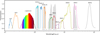 |
Fig. 1. In color, the main filter coverage between UV and mid-IR. For our SED fitting we have a total of 68 filters (colors). The five filters shown in grayscale on the background are the second option in case the main does not have an observation on the target. |
The J-PAS filter system effectively provides a low resolution pseudo-spectrum (from now on, J-spectrum) for every detected source and is particularly suited to study AGN (Abramo et al. 2012). In the ∼1 deg2 of the sky covered until now, the miniJPAS catalog contains more than 64 000 sources detected in the r band. This catalog is 99% complete up to r = 23.6 for point-like sources and up to r = 22.7 for extended sources (Bonoli et al. 2021). Point-like sources are defined as having CLASS_STAR > 0.9 in the morphological classification from SExtractor (Bertin & Arnouts 1996). Considering that we used the photometric data until r < 23.6, in this work, we do not provide morphological information about our sources.
miniJPAS offers different catalogs: single and dual modes. In single mode, the detection of sources is independent for each filter. This mode can be advantageous for obtaining information on faint sources with emission lines with a high signal-to-noise ratio (S/N). Because we are interested in obtaining a well-described shape of the optical SED, we used the dual-mode. In this catalog, the detection is performed in a reference band (r band), and the photometry of all other filters is forced to the reference aperture (fixed shape and centroid). From the dual catalog of miniJPAS we also picked two different photometries: AUTO and PSFCOR. The difference between them is that AUTO gives the magnitude within a Kron aperture, while PSFCOR is obtained in a smaller aperture and takes into consideration the differences in the point spread functions (PSFs) between the different filters (for details on the photometries definition, see Hernán-Caballero et al. 2021). In Sect. 3, we discuss and explain the choice of working with AUTO. We corrected all miniJPAS magnitudes for galactic extinction using the color excess E(B − V) calculated from Bayestar17 (Green et al. 2018) for each filter (for details, see López-Sanjuan et al. 2019).
2.2. X-ray selection
We selected the sources in the X-rays because it is an efficient method to search, in a wide range of redshifts, AGN with different luminosities that can be missed in other bands in the cases where the host galaxy dominates that flux (see Brandt & Alexander 2015, for a review). In the past years, the EGS field has been studied with profound X-ray observations from Chandra (Laird et al. 2009; Nandra et al. 2015) and shallower and wider observations from XMM-Newton (Liu et al. 2020). All sources detected during these observations have been cataloged. The catalogs provide X-ray fluxes in the soft (0.5−2 keV) and hard (2−10 keV) bands.
We compiled these data in a unique catalog, keeping the deepest observations for the sources with multiple detections. For the two Chandra catalogs, we crossmatched sources within two arcsec. Since XMM-Newton has a lower spatial resolution than Chandra, we used five arcsec of maximum separation for the crossmatch between Chandra and XMM-Newton sources. We also removed the spurious sources detected in Laird et al. (2009) following Nandra et al. (2015) and spectroscopically confirmed stars. Finally, we obtain a catalog of 4928 unique X-ray sources detected in ∼6 deg2 around the EGS field (1617 sources with Chandra observations and 3311 for XMM-Newton). Figure 2 shows a sky map of the X-ray compiled catalog and the miniJPAS footprint. The original catalogs also provided reliable counterparts, obtained using likelihood estimation analysis and deep optical/IR photometric data (for details, see Laird et al. 2009; Nandra et al. 2015; Liu et al. 2020) and only ∼2% of the sources do not have any optical/IR counterpart. One-third (1661) of our unique X-ray sources lie within the miniJPAS footprint and have a reliable optical/IR counterpart.
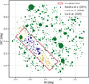 |
Fig. 2. Sky map of the X-ray sources on and around the miniJPAS footprint (red box). Each dot represents an X-ray source in our compiled X-ray catalog, color-coded to show its original catalog. The size of the dots is proportional to their total X-ray flux measured in 0.5−10 keV. |
We crossmatched these counterparts with the miniJPAS dual-mode catalog, up to r < 23.6 mag, obtaining 741 matches. When available, we added a confident spectroscopic redshift value from DEEP2 DR4 (Newman et al. 2013) and SDSS DR16 (Ahumada et al. 2020) using the optical/IR position and searching within a radius of one arcsec. We found robust redshift values for 430 of them (i.e. ZQUALITY ≥ 3 for DEEP2 and zWarning = 0 for SDSS). We also excluded sources with any type of flag in all the miniJPAS narrow filters. These flags can be from the extraction process (close neighbor, saturated pixel, too close to a boundary, tiles overlap, between others) or because the images were affected by different technical problems in the CCD or telescope (see Bonoli et al. 2021, for details on flags). Finally, we are left with 370 sources with X-ray fluxes, optical photometry, and a reliable redshift value. In Table 1, we show the numbers of sources in detail for each cut. The selection done is generous to include all types of sources, but we exclude a posteriori sources whose light is dominated by the galaxy host or the AGN, and thus the determination of their physical parameters is unreliable.
Total X-ray sources in the EGS fields and our sample selection.
2.3. X-ray flux correction
The X-ray photons suffer a photoelectric absorption that can be modeled depending on the hydrogen column density (NH). This absorption can be intrinsic to the source, occurring before the photons escape the host galaxy, or local, due to the interstellar medium (ISM) in the Milky Way (MW).
Since the X-ray AGN photons originate from a nonthermal process, they can be modeled with power-law spectra, and we can predict the loss of photons for a given power-law index, redshift, and intrinsic NH. Because the response curve of each X-ray telescope is different and can change during its useful life, this relation also depends on the instrument and date of observation.
To estimate NH, we used the Hardness Ratio, HR =  , where H and S are counts in the soft and hard bands, respectively. The hard band is measured in the 2−10 keV range, while S is in the 0.5−2 keV range. We use the software PIMMS2 to predict how HR changes with redshift at a fixed NH and photon index3 (Γ) for Chandra and XMM-Newton main cameras, and the representative observation date for each log. As an example, we show these predictions for Chandra sources with lines in Fig. 3. A similar approach to obtain NH from HR was employed in Marchesi et al. (2016).
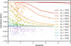 |
Fig. 3. Hardness ratio as a function of redshift for Chandra sources in our sample (dots). The solid lines show the value of the corresponding column density, NH, for a fixed Γ = 1.4. The color of each source corresponds to the assigned NH (values in cm−2). |
We computed the bayesian HR using the program Bayesian Estimation of Hardness Ratios (BEHR; Park et al. 2006) for all the sources (shown as dots in Fig. 3). Finally, we selected the nearest curve for each source, estimating the closest value of intrinsic NH for them.
The flux correction for the MW absorption was already performed in the original catalogs. Then we just apply the correction for the intrinsic absorption to obtain the intrinsic values of X-ray flux on the soft and the hard bands. We use PIMMS, adopting the estimated intrinsic NH. In Fig. 4, we show the flux corrected for intrinsic absorption following the procedure outlined above as a function of the detected flux for the soft and the hard bands. As expected, absorption affects the hard band less than the soft band.
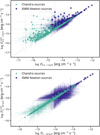 |
Fig. 4. Intrinsic X-ray fluxes as inferred after the NH correction vs. measured fluxes in the soft (0.5−2 keV, upper panel) and hard (2−10 keV, lower panel) bands. |
In Fig. 5, we show the redshift distribution for all the X-ray sources with spectroscopic redshift measurements in the EGS field (1394). This distribution drops significantly after z = 1.5, showing a small number of sources after z = 3. We decided to cut in z = 2.5 our sample with miniJPAS detection (370) to avoid spreading our sample at higher redshifts with few sources (see Table 1). This cut defines our final sample: 347 X-ray sources with spectroscopic redshifts and miniJPAS photometry (flagged). This sample is shown in red in Fig. 5. In this figure, we also show the histogram for the estimated intrinsic NH and the distribution of X-ray absorption-corrected luminosities for all the sources in the EGS field and our final sample. While the distribution of NH is similar for both, our sample does not resemble the shape of the LX distribution for the complete EGS field. Values can be found in Table 2.
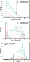 |
Fig. 5. Distributions of spectroscopic redshifts (upper panel), intrinsic column density NH (middle panel), and hard X-ray luminosity (lower panel) for all sources in the EGS sample (green) and our final sample with miniJPAS detection and good photometry used in this work (red). |
Sources analized in this work.
2.4. UV/IR data and optical spectra
In order to build a complete SED and to fit diverse host galaxy and AGN models, it is necessary to have multiwavelength data. Because of this, we included in our analysis all the available photometric data from ultraviolet (UV) and infrared (IR) full-sky coverage surveys when were available (Fig. 1). The chosen filters cover UV to mid-IR with up to 68 bands as detailed below. This selection was made to cover the rest-frame UV to near-IR fluxes up to z = 2.5 for all sources. This will allow a good estimate of the SED, especially on the host galaxy emission.
For UV, we crossmatched our catalog with GALEX GR6/7 (Bianchi et al. 2014) within a radius of five arcsec. The chosen radius considers the PSF and astrometry accuracy of the instrument. We added the fluxes in the near UV (1350−1750 Å) for 257 sources and in the far UV (1750−2800 Å) for 207 sources in our final sample. This gave us a good estimation of UV photons from the sources for a majority of our sample (∼80%), and only 18% of our close sources (z < 0.5) do not have rest-frame UV data. We corrected the UV fluxes for galactic extinction using the coefficients from Yuan et al. (2013).
We used the J, H, and Ks bands from Moles et al. (2008) to cover the near-IR range. The ALHAMBRA near-IR survey covered different fields of interest across the sky, and in particular, the ALHAMBRA-6 field overlaps with our field. We found photometry on all these bands for 120 sources of our sample. For the sources without an ALHAMBRA detection, we searched the Palomar WIRC original AEGIS catalogs (Davis et al. 2007). We added J and Ks photometry from this catalog for 67 and 178 sources, respectively. Overall, we have at least 298 sources (∼87%) with some flux on the NIR bands.
For the mid-IR, we used the Spitzer IRAC and MIPS photometry from Barro et al. (2011). The four filters from IRAC gave us coverage between 3 and 10 microns. We found photometry for 273 of our sources for IRAC1 and 2, while 271 for IRAC3 and 272 for IRAC4. In the case of MIPS, we included 24 and 70 μm photometry for 251 and 135 sources, respectively.. For the ones without observations made from Spitzer, we used CatWISE2020 (Marocco et al. 2021) to obtain the fluxes for the W1 and W2 bands (3.4 and 4.6 μm). To get the fluxes for W3 and W4 (12 and 22 μm), we used AllWise (Cutri et al. 2013). We did a color correction following the recommendation by All-WISE website4. We used the published color correction from Wright et al. (2010), and the observed color W2 − W3 to estimate the power-law index for each source and applied that color correction when the magnitudes were converted into fluxes. Upper limits were added for undetected sources. In the case of W3, we also consider this filter for 262 sources (∼75% of the total sample) since this filter is in the gap between IRAC and MIPS (see Fig. 1). In total, we have at least 346 sources with some photometry between 3−10 μm, and 322 with photometry at 22−24 μm.
We also searched for available spectra for our optical counterparts of each source within one arcsec. We used the spectra in the SDSS DR16 public archive5 and from the DEEP2 survey (Newman et al. 2013). In the case of SDSS, we found that 101 sources have at least one spectrum. For sources with more than one SDSS spectrum, these were stacked to improve the S/N, obtaining a median spectrum for each source. For DEEP2 data, we used the 1-d spectra, obtained throughout a variant of Horne optimal extraction (see Newman et al. 2013, for details), for 111 sources. Since the DEEP2 spectra are not flux calibrated, we corrected them, considering the CCD sensitivity6 as a function of wavelength. With that correction, we can better recover the correct shape of the spectra. This region of the sky was also targeted with MMT (Coil et al. 2009; Yan et al. 2011). The authors shared with us their reduced spectra for 111 sources in our sample. Both SDSS and MMT spectra were flux calibrated. Considering all these spectra, we found at least one spectrum for 269 miniJPAS sources. Details on the final spectra and their analysis can be found in Sect. 4.
3. Data analysis: Spectral energy distributions
The multiwavelength emission of galaxies can provide hints about their principal components: stars, dust, and gas, among others. Modeling the SEDs with different templates allows us to measure the physical properties of the host galaxy, disentangling the different components. Since our sources are active galaxies, we must also consider their nuclear emission. To perform the SED fitting, we used Code Investigating GALaxy Emission (CIGALE7; Burgarella et al. 2005; Noll et al. 2009; Boquien et al. 2019) with the X-ray module added by Yang et al. (2020) that makes it possible to include an AGN component in the X-rays.
CIGALE is a solid SED fitting code prevalent in galaxy evolution analyses and has become more popular in the last years in AGN studies. The new features incorporated in the last update added the ability to consider the extinction of UV-optical from polar dust and the X-ray photons (for details, see Yang et al. 2020). Recent works established CIGALE’s efficiency in recovering specific physical parameters of the host galaxy and AGN. Mountrichas et al. (2021) used a set of mocks AGN and demonstrated that CIGALE could disentangle the AGN/host emission finding an agreement between the true values of SFR and M⋆ and those recovered from the fitting. They also used an X-ray-selected sample with X-ray to far-IR photometry. They showed that CIGALE is powerful enough to correctly classify between type I and type II AGN, considering inclination and polar dust. Some parameters’ accuracy can be improved by adding more bands; for instance, SFR is more robust when far-IR photometry is included. In our case, we did not include Herschel data in the fitting because the available data in the field was not deep enough. Even without far-IR photometry, CIGALE can obtain reliable SFR for X-ray-selected sources with spectroscopic redshift using the rest of photometric data (Masoura et al. 2018).
For our work, we construct the SED of each source using the redshift and photometric fluxes from all the available bands described in Sect. 2 and Fig. 1 (2−10 keV, 0.5−2 keV, FUV, NUV, the 56 miniJPAS optical filters, J, H, Ks, IRAC1-4, WISE3, MIPS1, MIPS2). For sources without detection in IRAC bands, we used the WISE bands (W1, W2, W4). In particular, for X-rays, CIGALE requests intrinsic fluxes. We set the upper limits for nondetected bands following the completeness studies from their original catalog. This wavelength coverage allows us to build a good rest-frame SED for the AGN and host galaxy, even at redshift 2.5.
CIGALE uses independent modules that model a unique physical feature or process. For each parameter of these modules, CIGALE builds a prior from a given grid of parameters. To choose the modules and the grid of parameters, we followed Mountrichas et al. (2021) because of the similarity of our sources. In Sects. 3.1 and 3.2, we describe each module used for the host galaxy and AGN and the values adopted for the parameters. A full description of modules and parameters used as input is given in Table 3. CIGALE also estimates two values for each output parameter: one from the best-fit model (called best value) and another one that weighs all grid models (called bayesian value). These weights are based on the Bayesian likelihood exp(χ2/2) associated with each model.
Parameters and values for the modules used with CIGALE.
3.1. Host galaxy emission
For the stellar component, we use a τ-delayed SFH. This parametrization is very versatile because it allows a smooth SFR with a similar shape as the average SFR density across cosmic time (Madau & Dickinson 2014) and depends on the time at which the SFR peaks (τ) for each source. The functional form is SFR(t) ∝ t τ−2exp(−t/τ), and after the maximum at t = τ, the SFR smoothly declines. We also include the possibility of a recent burst following Małek et al. (2018). The stellar templates are from Bruzual & Charlot (2003) and an initial mass function from Chabrier (2003), with a fixed solar metallicity to avoid degenerations. The stellar emission is attenuated following the Calzetti et al. (2000) law, and the dust emission is modeled with the template from Dale et al. (2014). Since our photometric data includes narrow filters, emission lines typical of star-forming regions can be detected (Martínez-Solaeche et al. 2022). Because of that, we added a model for nebular gas that uses nebular templates from Inoue (2011), choosing a width of 300 km s−1 for narrow emission lines. CIGALE also includes the possibility for low-mass and high-mass X-ray binaries (LMXB and HMXB) to fit the X-ray emission.
3.2. AGN emission
For the active nuclei, we use the Skirtor model included in X-CIGALE (Yang et al. 2020). We followed Mountrichas et al. (2021) to model the different obscuration for Type I and Type II AGN, setting two possible inclinations (30 and 70°) and a grid of values for the polar dust. We also set two posibilities for the torus optical depth at 9.7 μm (3.0 and 7.0). The accretion disk spectrum used as the primary energy source for the AGN emission is from Schartmann et al. (2005).
The AGN fraction, fracAGN, can be used to compare the emission of the host galaxy versus the AGN. This parameter is the fraction of the total IR emission from the AGN. We used a grid to cover the possible values (0.01, 0.1, 0.2, ..., 0.9, 0.99) leaving the possibility of obtaining a SED entirely dominated by the host galaxy or the AGN.
The X-ray module helps to constrain the UV emission from the accretion disk using the αox − L2500 Å relation, and for it, we set an ample grid for possible values of αox (−1.9, −1.75, ..., −1.15, −1.0; Xu 2011; Lusso & Risaliti 2016). Considering that our X-ray fluxes are corrected by intrinsic absortion, we set a photon index typical for AGN of Γ = 1.8.
3.3. Fitting
We ran CIGALE for our final sample (347 sources) using the modules and parameters described in Table 3. The number of models computed per source by CIGALE is 5 544 000. We ran it for two different types of miniJPAS photometry: AUTO and PSFCOR.
Both photometries have their pros and cons. The PSFCOR considers issues like point-spread function variation on the focal plane for different dates, biases on filters, and aperture correction, among others. However, its small aperture gives a value below the galaxy’s expected total flux. AUTO provides a closer value to the total flux, but it can be noisier due to a bigger aperture. To compare the SED fitting results of both photometric fluxes, we scale the J-spectra obtained from PSFCOR using the  as the reference value.
In Fig. 6, we show the distribution of reduced χ2 for the SED fitting with both types of photometries. Both distributions are similar, showing good fits, with a high number of sources near one and a decreasing tail beyond three, being AUTO the one with more sources near one (expected since AUTO is noiser). For a deeper comparison between the results for both photometries, see Appendix A.
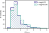 |
Fig. 6. Histograms of reduced χ2 for the SED fitting performed using two different sets of magnitudes extracted from miniJPAS catalogs, AUTO and PSFCOR (see Sect. 3.3). |
Since, in our analysis, it is necessary to obtain an estimation of the properties of the host galaxy and the AGN, we excluded the sources dominated by only one component (i.e., pure-AGN or pure-galaxy). Mountrichas et al. (2021) and Buat et al. (2021) show that, for a given parameter, if there is a large difference between the best value and the Bayesian value, the estimation of such parameter is not reliable. Following this idea, we can exclude the sources where the difference between parameters is bigger than one order of magnitude for M⋆, SFR, and LAGN. In other words, we can only keep sources with  ,
,  and
and 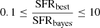 . In Fig. 7, we show the reliability of our fits using these criteria. The parameters obtained with the different miniJPAS photometries show similar distributions, centered in one with small dispersion. The choice of 1 dex as limit was made to exclude all outliers. In Appendix A, we show no significant difference between the two photometries, besides that AUTO has marginally smaller relative errors. From now on, we only present the results obtained using AUTO. We also remove the sources where the AGN luminosity is close to zero. Finally, following these criteria, we remove 39 sources (∼11% of the sample). We are left with 308 sources with reliable measurements of the AGN and the host galaxy components. Examples of SED fitting and its close up to the miniJPAS J-spectra are showed in Fig. 8.
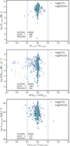 |
Fig. 7. Criteria used to exclude the sources with unreliable physical parameters. The bayesian values for M⋆ (upper panel), SFR (middle panel), and LAGN (lower panel) are plotted against the ratio of best values over Bayesian. The distribution is centered at 1. The solid vertical lines mark the limits of 0.1 and 10 adopted in this work (see Sect. 3.3 for details). The different colors show the parameters and ratios obtained assuming different magnitudes as input. The number of sources between and outside the limits is reported in the lower part of the plots. |
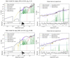 |
Fig. 8. Examples of SED fitting using CIGALE and their residuals. Pink circles show the photometry for each band used. Green triangles are upper limits. The black dashed line is the composite model, and the color lines are the individual components of the composite model. Left: full range of wavelengths, from X-ray to IR. Right: close up on optical miniJPAS J-spectrum. |
4. Data analysis: Optical spectra
The emission lines in AGN spectrum can provide information about their obscuration and the SMBH properties. Broad lines are observable for Type I, while narrow lines are present in both types. Typically, we can assume that the SMBH’s gravitational field dominates the gas cloud motion in the broad-line region (BLR). Thus, the width of these lines is related to the virialized mass of the SMBH. A spectral fitting is necessary to obtain a good measure of the width, considering all other features typical of AGN. In this section, we discuss the spectra used, the fitting process, and the estimation of MBH.
4.1. Fitting
We described the spectra used in Sect. 2.4, but in summary, at least one spectrum was available for 269 sources of our initial sample. We did a cut of a mean S/N > 3 on these spectra. After we fit them, we obtained an acceptable FWHM of broad region lines of 113 AGN for our final sample. When more than one spectra were available for the same source, we selected the one with the highest S/N.
We used PyQSOFit (Guo et al. 2018) to fit the continuum, iron emission, and emission lines of the AGN. We fit the spectra with a combination of continuum and line emission. We used a polynomial for the stellar continuum and a power law for the AGN continuum, and we also included iron emission. In the case of narrow lines, we allow one Gaussian with the same width for all the narrow features. Broad lines can be very complex because of the presence of asymmetries; in these cases, the width estimated by only one Gaussian gives systematically larger widths (Shen et al. 2008). Due to this overestimation, we allow between one and three Gaussians depending on the line following Rakshit et al. (2020). The multicomponent Gaussian used to fit the narrow and broad emission lines are listed in Table 4. In particular, we measured the FWHM of the broad component of Hα, Hβ, MgII, and CIV and the luminosity at 1350, 3000, and 5100 Å. For the DEEP2 spectra that is not flux calibrated, we scaled them to the luminosity (1350, 3000, and 5100 Å) of the closest narrow-band filter from miniJPAS photometry.
Emission lines used in the spectral fit.
We set limits for the width of the emission lines fitted. To distinguish between broad and narrow lines, we used a value of 1000 km s−1. The upper limit for the broad lines was 10 000 km s−1. These limits come from the width bimodal distribution shown for X-ray-selected AGN lines (Menzel et al. 2016).
4.2. BH mass estimation
Although σ seems to correlate better with the masses calculated from the reverberation method, we use FWHM instead. The main criterion for this choice is that σ is too sensitive to noise on the wings of the emission lines (Shen & Liu 2012). To estimate the error in the FWHM, PyQSOFit uses a Monte Carlo approach to fit random mock spectra and obtain the uncertainties considering the flux errors and systematic errors for multiple decomposing components.
Several works calibrate the virial relation from a single-epoch spectrum (see Shen & Liu 2012, for a compilation). Different lines have slightly different calibrations. For our MBH estimation, we used the coefficients from Assef et al. (2011) for the Balmer lines (Hα and Hβ); Vestergaard & Osmer (2009) for MgII; and Vestergaard & Peterson (2006) for CIV. We used the following equation to estimate the black hole masses, with an overview of the coefficients in Table 5,
 (1)
(1)
Coefficients used for different emission lines.
To obtain MBH uncertainties, we propagate the FWHM and luminosity uncertainties in the Eq. (1), including the dispersion of the original fit where the coefficients a, b, and c were calculated. Similar to the spectra selection, to estimate MBH when more than one line was present, we selected the one with higher S/N (if the corresponding fit was acceptable). Examples of spectral fits are shown in Fig. 9. Finally, we obtained black hole masses for 113 sources in our sample with reliable SED fitting. Sixty of these masses were obtained using SDSS data, 43 from MMT and ten from DEEP2.
 |
Fig. 9. Examples of spectral fitting using PyQSOFit, and their residuals. On gray the spectra observed, at rest-frame wavelength. Continuum was fit as a polynomial, showed in orange. On cyan, the Fe emission. On blue, the emission lines fitted in the process to obtain FWHM of the BLR. |
These masses are similar to those obtained by Rakshit et al. (2020), as shown in Fig. 10. We do not find a systematic shift between our masses and theirs. The difference for some sources may be related to the difference in the fitted spectra; while they use the best SDSS spectra, we use SDSS stacked spectra or a different epoch MMT spectra, if the S/N was higher than SDSS. Because our work also considers stacking and adds spectra from other telescopes, we obtained BH masses for more sources in our sample. Another way to obtain spectra independent MBH is by measuring the broad line directly from the J-spectra. Chaves-Montero et al. (2022) explored this possibility with promising results compared with Rakshit et al. (2020). While this work can be applied to extensive areas in the future of JPAS, it is currently limited to sources brighter than r < 21 and MBH > 108 M⊙.
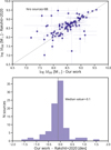 |
Fig. 10. Upper panel: comparison between our estimation of the black hole masses and the ones estimated by Rakshit et al. (2020) for the 88 sources in common. Bottom panel: histogram of the logarithmic difference of the BH masses. |
5. Physical properties of AGN and host galaxies
Until now, we have recovered reliable values of properties for 308 AGN and their host galaxies from SED fitting. We also estimate MBH for a subsample of 113 sources. In this section, we show the distributions of these properties and the derivation of additional parameters that depend on them.
5.1. Distributions of physical properties
In Fig. 11, we show the distributions of M⋆, SFR, and LAGN for the entire sample of 308 miniJPAS sources for which these parameters have been derived (red) and the subsample of 113 sources for which we also have a reliable measurement of MBH (green). The values for individual sources can be found in Table 6. While the distribution in M⋆ is very similar for the two samples, the subsample with measured BH masses is biased toward higher LAGN and SFR.
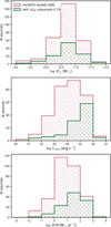 |
Fig. 11. Histograms of the physical parameters estimated with the SED fitting (M⋆, LAGN and SFR). In red is the full sample while in green is the subsample with an estimation of MBH using the corresponding spectra. |
Physical properties of the galaxies in the entire sample of 308 galaxies.
To quantify the difference, we performed a Kolmogorov–Smirnov test to check the null hypothesis that the subsample was drawn from the same probability distribution of the larger sample. We obtained a p-value smaller than 1% for LAGN and SFR. While we cannot discard the null hypothesis for the M⋆ (p-value ∼ 0.88), we can say our subsample shows a bias toward high values of LAGN and SFR. The origin of this bias could be ascribed to the fact that it is easier to obtain well defined spectra for more luminous sources, which in turn are powered, on average, by more massive black holes.
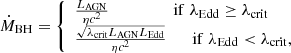
5.2. Eddington ratios and proxies for the accretion rates
We derived estimates of the Eddington ratios, which is a fundamental parameter for constraining BH cosmological evolution (Sect. 1), for the subsample of 113 sources with BH mass estimates based on BLR widths. The distribution of λEdd for this subsample is shown in the upper panel of Fig. 12. This distribution shows a clear peak at around λEdd ∼ 0.1, with a steep fall off at larger Eddington values, and a slightly less abrupt one at lower Eddington ratios.
 |
Fig. 12. Distribution of accretion rates derived in this work. Upper panel: histogram of Eddington accretion rate (λEdd) for the sources with measured MBH. Middle panel: histogram of the specific accretion rate (λsBHAR, typically used as proxy of λEdd), for both the sample with measured BH masses and the full miniJPAS sample. A difference in the shape of distributions can be seen for the subsample with measured BH masses by comparing the green histograms in the upper and middle panels. Lower panel: plot of the relation between λsBHAR − λEdd. While they are defined to be equal, we found a poor correlation value and a systematic shift from the 1:1 relation in their linear regression (plotted as gray with 1-σ uncertainties in pink). |
The Eddington ratio distribution of our sample is significantly different from other works (Vestergaard & Osmer 2009; Nobuta et al. 2012; Lusso et al. 2012). In particular, we compared with Lusso et al. (2012) because both samples were X-ray selected, and physical properties were estimated with similar methods (SED and broad-line fitting). The Eddington ratio distributions have a difference of 0.5 (0.7) dex for median (mean) values. The difference is likely due to the combination of selection effects and estimation of LAGN in each study. Both samples are similar in LX, but their optical spectra are deeper, reaching higher magnitudes than our work. Second, their estimation of LAGN comes from the bolometric AGN emission from 1 μm to 200 keV; in our case, LAGN only corresponds to the integrated accretion disk luminosity (agn.accretion_power in CIGALE). In our sample, we registered a difference in 0.3 dex comparing our LAGN with the higher values of bolometric AGN luminosity calculated from CIGALE.
For completeness, following other works in the literature (e.g., Aird et al. 2018), we also compute distributions using alternative measurements of the Eddington ratios, namely λsBHAR, defined as:
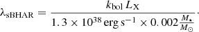
For comparison, we adopt kbol as 25. We note that in this case we can include all sources from our AGN sample as λsBHAR does not rely on independent BH mass measurements. This rate is defined to be λsBHAR ≈ λEdd using the strong hypothesis that the mass of the SMBH scales directly with the total stellar mass of the host galaxy, as MBH ∼ 0.002 M⋆ (Marconi & Hunt 2003; Aird et al. 2018).
We show the λsBHAR for the entire miniJPAS X-ray sample (red histogram) and also for the subsample with measured BH mass (green histogram) in bottom panel of Fig. 12. We observe a difference between the λEdd and its proxy λsBHAR with the latter being ∼0.6 dex larger. When we compare these distributions with a Kolmogorov–Smirnov test, we obtained a p-value lower than 1%, further suggesting that these distributions are significantly different, shedding some doubts on the actual suitability of λsBHAR in constraining BH accretion rate models.
While these two rates are defined to be similar, the difference is outstanding. The strong assumption used to acquire an λEdd without a measured BH mass can explain this difference since our sample shows a strong scatter for the MBH − M⋆ relation. In Sect. 6, we discuss the nature of the scaling relation for our selection and its possible evolution across cosmic times.
5.3. AGN properties
In Sect. 1, we mentioned the importance of obtaining BHAR distributions. This rate in physical units (ṀBH) can be derived starting from the AGN accretion luminosity (LAGN). This is possible by assuming a proportionality between LAGN ∝ ṀBH/ṀEdd, for all Eddington ratios (λEdd). Given that we have an estimate of MBH, we followed Merloni (2004) and adopted a broken power-law, connecting the low accretion rate (radiatively inefficient) regime with the high accretion rate one. The break is given at λcrit = 3 × 10⁻² (Merloni 2008). Imposing continuity at λcrit, yields the following equation:
 (2)
(2)
where η is the radiative efficiency, assumed as 0.1.
We applied Eq. (2) to derive the BHAR in physical units for our sources with measured MBH. Figure 13 shows ṀBH as a function of the AGN luminosity, color-coded by BH mass and the distribution of ṀBH. The shape of the distribution for higher values is, as expected, similar to the distribution of λEdd (see Fig. 12). For lower values, it is less steep than λEdd, as a consequence of the change in the accretion regime. It is also less steep than a distribution derived from ṀBH ∝ LAGN, with a σ = 0.75 instead of σ = 0.95. With Eq. (2), we recovered the change in the accretion mode, obtaining higher values of ṀBH than the typical accretion (as seen in the both panels of Fig. 13). Our ṀBH also shows similar correlations with SFR as Delvecchio et al. (2015) and Masoura et al. (2018), even with the two regimes.
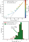 |
Fig. 13. Upper panel: accretion rate depending on LAGN. The solid line is the typical accretion rate assuming a linear dependence with LAGN, and it is equal for our sources with λ > λcrit. For the rest of the sources, the dispersion comes from the dependence with MBH, which is color-coded. Lower panel: histogram of the estimated BH accretion rates. |
6. Stellar and BH mass evolution
In the previous sections, we derived reliable stellar and BH masses for 113 miniJPAS sources with z < 2.5. These two quantities are compared, with the associated uncertainties, in the upper left panel of Fig. 14. For reference, we also included some local MBH − M⋆ scaling relations, like MBH = 0.002 M⋆ used to define λsBHAR and based on Marconi & Hunt (2003). We plot also the relation derived by Shankar et al. (2020), based on the BH masses measured from the velocity dispersions from Savorgnan et al. (2016). Since this method of measuring masses can have biases due to, for example, the spatial resolution of the instrument used, we also included an unbiased relation proposed by Shankar et al. (2016). We also included the parametrization obtained by Georgakakis et al. (2021), where they presented an empirical model for BH populations in large cosmological volumes.
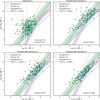 |
Fig. 14. Upper left panel: the observed MBH − M⋆ relation for all the 113 sources in our sample, at the observed redshift. Green solid dots are the value of masses for each source, with associated uncertainties, while contours are the distribution of these dots. In all panels, we show the expected local MBH − M⋆ scaling relations: in turquoise the 0.002 M⋆ from Marconi & Hunt (2003); in green the relation from Savorgnan et al. (2016) with uncertanties at 1-σ; in purple the unbiased version from Shankar et al. (2016) with uncertanties; and in brown the parametrization by Georgakakis et al. (2021). The other three panels show the forward modeling of our sources to z = 0 using different methods. Upper right panel: the most basic model, with constant rates (Scenario 1). Lower left panel: the model with a variable rate following the SFH (Scenario 2). Lower right panel: the model with a variable rate following the SFH and the energy limit for the black hole accretion (Scenario 3). See Sect. 6 for details. We also show the number of sources and the Pearson correlation value on each bottom right corner. |
Our sample does not seem to follow any of the local relations. Overall, a correlation between M⋆ and MBH is not statistically significant with a Pearson correlation coefficient of only ∼0.3. This work is not the first to find overmassive BH compared with the local MBH − M⋆ scaling relation. For example, Ding et al. (2020) studied a sample of AGN between 1 < z < 2, and they found MBH almost three times more massive than those predicted by typical local MBH − M⋆ relations. It is clear that both physical effects as well as selection effects play a role in causing such apparent discrepancies.
In any case, thanks to our comprehensive multiwavelength analysis, we also have reliable estimates of the SFR and the BHAR for all the sources in our sample. Merloni et al. (2010) obtained stellar and black hole masses, and their SFR and BHAR for a sample similar in size (∼100) of X-ray-selected AGN at z ∼ 1.2. They showed that, assuming a constant value for the rates, an evolution of the sources for 300 Myr brings to a reduction of the scatter of the relation, and a new position in the MBH − M⋆ plane closer to the local scaling relations.
A simple constant model for the rates can be a valid assumption for evolution within short times (like nearby sources). Still, a constant value of SFR across longer times is likely an oversimplification. In fact, a galaxy will increase its stellar mass during its lifetime following a SFR that is not constant and that depend on the gas reservoir and its cooling time. This reservoir change over time by the effect of, for example, supernova, AGN feedback and/or mergers (Granato et al. 2004; Lapi et al. 2006; Monaco et al. 2007; Fontanot et al. 2020). A similar situation occurs for the SMBH mass. There are hints pointing out that the BH accretion rate shows a similar trend as the one observed in the star formation up to the peak epoch of galaxy-AGN coevolution (z ∼ 3, e.g., Madau & Dickinson 2014; Aird et al. 2015). Nevertheless, this evidence is valid only for active black holes, where the accretion can be measured. To take into account the AGN duty cycle (Hickox et al. 2014), a more complex approach is necessary, based on continuity equation approximations (e.g., Small & Blandford 1992; Shankar et al. 2013), as well as direct measurements of average BH accretion rates across large samples of active and inactive galaxies (e.g., Yang et al. 2018; Carraro et al. 2020).
We applied these basic ideas and performed forward modeling of our source properties to estimate the host galaxy stellar and BH masses that each source will have at z = 0, assuming an isolated evolution (merger-free). While mergers can be the main triggering mechanism of AGN activity for luminous sources (Treister et al. 2012; Goulding et al. 2018; Gao et al. 2020), also observational studies and simulations suggest that mergers are not the dominant source of BH growth globally (Aversa et al. 2015; Steinborn et al. 2018; McAlpine et al. 2020), and even galaxies without major mergers since z ∼ 1 follow the MBH − M⋆ relation (Martin et al. 2018). In any case, while our isolated evolution does not include the possibility of mergers, the measured accretion rate can be the result of a previous interaction of the host galaxy with their surroundings.
We considered three different evolving scenarios to model the late evolution of BHs and their host galaxies down to z = 0: (1) constant growth, (2) variable growth, and (3) variable growth with an energy limit. Each model starts from the values of M⋆ and MBH measured at the observed z and from the estimated rates (SFR and BHAR). Then, using a time step of 100 Myr, the model predicts the increment for both masses for each bin in time.
The first scenario (Scenario 1) is the simplest one, where the rates are kept constant across time and are equal to the measured SFR and BHAR at the redshift of the sources up to z = 0. This approach is similar to what was considered in Merloni et al. (2010).
The second scenario (Scenario 2) incorporates an evolution for both rates. For the SFR, we follow the SFH derived from the SED fitting. Instead of using analytical law for the BH growth (like Bondi accretion) and modeling the BH feedback, we choose a more straightforward approach. Aird et al. (2015) shows that SFR density is related to the BHAR until z = 3 for active galaxies, obtaining the BHAR from the X-ray luminosity function for AGN. Newer studies, like Yang et al. (2018) and Carraro et al. (2020), show that this average relation is also valid for samples in different stages of their duty cycle (detected and not detected in X-ray). Since all this evidence suggests that the SFR’s shape is similar to BHAR at least until z = 3 (Aird et al. 2015), we used the τ-delayed model of SFH of each source to obtain their BHAR at each time step. To scale the BH accretion history, we used the observed value of BHAR at observed z.
The third scenario (Scenario 3) is similar to the second one, but a simple energy budget limits the BHAR. The BH is temporarily switched off if the total energy released by the AGN is larger than the gravitational binding of the host galaxy. This approach emulates a duty cycle and gives each source the possibility of periods of nonnuclear activity while the SF continues. While the shape of the relation is similar in studies for galaxies with diverse duty cycles (Yang et al. 2018) and for only active galaxies (Aird et al. 2015), the peak of the average BHAR at z = 2 for AGN is three times bigger. Our sources are X-ray detected, so the accretion activity is high at the observed z. Thus, using these BHARs to model the accretion across history (as in scenario 2) can produce overmassive BHs; considering a duty cycle is fundamental for the evolution of each source (not averaged). In other words, each source has an energy budget and an active BH for the zero time step (equal to the observed z). For the following time steps, if the energy limit allows it, the BH will be active, accrete, and follow the BHAR-SFR relation; if not, the BH will not have activity while the host galaxy will continue to form stars. This scenario better represents the normalization limits for the empirical BHAR-SFR relation for an X-ray-selected sample.
For Scenario 3, we calculated the energy released by the AGN at each time, as ĖBH(t) = ηϵc2 ṀBH(t), where η is the radiative efficiency and ϵ is the coupling efficiency, and represents the energy fraction that couples with the surrounding medium. We used ϵ = 0.1 adopted as maximum value in Weinberger et al. (2017). This value is also representative of other feedback models (Harrison et al. 2018). For the gravitational binding energy,  , where r is a radius representative of the galaxy. We took it from the relation between M⋆-size from Ichikawa et al. (2012). This relation is independent of redshift and type of galaxy, and the radius is calculated for each bin in time. We used r = r90 since it contained 90% of the light, and we are using all the source’s light to estimate the M⋆. Because this, Mtotal(t) takes into account the most massive components inside the r90: M⋆(t) and Mhalo(t) up to that radius. Considering the initial M⋆, SFR and SFH, we calculated M⋆(t) at each bin. For Mhalo(t)|r, we used the M⋆ − Mhalo relation from Girelli et al. (2020). This Mhalo is the total mass of the halo, so we used a Jaffe profile8 and the total mass to recover the fundamental parameters of the halo mass distribution and integrate Mhalo(t)|r. After all the energies are calculated, we checked for each bin in time if EBH(t) ≤ Egb(t). If the energy is below the limit, the BH can accrete following the SFH. If not, the accretion stops and equals zero for that bin in time. The BH accretion can start again if the stellar mass increases because of high SFR; therefore, the gravitational binding is higher.
The results of the forward modeling in the three scenarios described above are shown in Fig. 14 (upper right, lower left and lower right, respectively). We performed a linear fit of the MBH − M⋆ relation evolved at z = 0, and in all three cases, the Pearson correlation coefficient factor increased substantially compared with the first panel.
With the simplest model (Scenario 1), the sources seem to follow a relation of 0.01 between masses, with a correlation factor of ∼0.8. While this can be promising, the constant rates bring an estimate of M⋆ and MBH considerably higher than those observed in the local Universe. While in the local Universe the highest values are MBH ∼ 1010 M⊙ (Bennert et al. 2021) and M⋆ ∼ 1012 M⊙ (Karachentsev et al. 2013), we predict masses 10 times higher.
Both BH and stellar masses distributions on the model following the Scenario 2 have slightly lower values than in Scenario 1. While M⋆ has values comparable to those observed in the local values, MBH keeps being too high.
The model with an energy limit for the BH accretion (Scenario 3) has the highest correlation coefficient factor (0.88) and masses closer to the local ones. Furthermore, our sample is closer to the dynamically measured relation (Savorgnan et al. 2016) and unbiased relation (Shankar et al. 2020) than the relation obtained from forwarding model (Georgakakis et al. 2021), with almost all its scatter inside the 1-sigma uncertantain of the dynamically measured relation. With this scenario, we show that imposing an energy limit on the BH decouples the link between rates for specific periods of their evolution being critical to reproduce the MBH − M⋆ relationships. This limit is effortless to compute and still capable of lowering the BH masses at redshift zero, signaling that our simple assumptions are reasonable.
Neither of the three scenarios was very sensitive to small changes in how ṀBH was derived. We ran them for the typical derivation ṀBH ∝ LAGN without significant changes in the correlation values. We also applied the scenarios to 100 sets of different rates as a sanity check. We started from the same initial measured masses, but we evolved these sources with SFR, SFH, and LAGN randomly sampled from a normal distribution centered in the mean value of our sample and with the same scatter. We found that for random samples, the evolution shows average correlation values significantly lower than our sample (∼0.5). Therefore, for our forward modeling is essential to set actual input rates for each source and will not produce the same results for random samples.
The forward models explained in this section are naive and straightforward by design, since they are based on a short set of observational inputs. The principal limitation is not having information about the gas reservoir of the galaxy; thus, accretion and star formation do not have a limit depending on how much gas is available. In this sense, our models are just a higher limit of how much the galaxy and its SMBH can grow. Nevertheless, we compared our results with a more complex evolution model, the Magneticum simulations9. Magneticum is a set of fully hydrodynamical cosmological simulations that can trace structures through cosmic time, with different resolutions and box volumes (details on Hirschmann et al. 2014; Teklu et al. 2015). In particular, we crossmatched our sources at observed redshift with the Magneticum/Box2, finding a similar stretch on the MBH − M⋆ relation at lower redshift on the evolved sources at z = 0.
7. Summary and conclusions
We studied the host galaxy and central BH properties of a sample of X-ray-selected AGN using narrow-band data from the miniJPAS survey together with available multiwavelength data from UV to mid-infrared. We obtained robust parameters from SED fitting for 308 sources. We also measured BH masses from single-epoch spectra for a subsample of 113 sources. For this subsample, we provided reliable estimates of BH accretion rates and Eddington ratios. We also studied three different possible evolutionary scenarios for the subsample with BH mass estimates. We summarize below the main results of our work:
-
The distribution of the Eddington ratio for our sample overgrows to lower values, peaking at λEdd ∼ 0.1, and decreasing toward λEdd ∼ 0.0001 (see the upper panel of Fig. 12). Since our sample is biased toward high-luminosity AGN, the distribution at λEdd < 0.01 needs to be studied with complete samples down to a luminosity of 1042 erg s−1 in the future.
-
We found that the distribution of Eddington ratios is on average about 0.6 dex smaller than its commonly used proxy λsBHAR (see Fig. 12 for a comparison). This difference must be studied in detail and highlights the importance of using high-quality photometric and spectroscopic data to derive physical parameters of accreting black holes.
-
We derive accretion rates in physical units that depend on the expected radiative efficiency (see Eq. (2) and Fig. 13), using the estimated accretion luminosities and BH masses, obtaining less scatter than the accretion rates derived with a linear relation with LAGN.
-
We do not find a correlation between the measured BH mass (MBH) and the galaxy stellar mass (M⋆) for the sources in our sample (upper left panel in Fig. 14).
-
The fact that in our sample we measure overmassive BHs for their stellar masses compared to the local relations can be either ascribed to biases on LAGN or to evolutionary effects. To test this second hypothesis, we applied forward modeling for our sources to the present time, considering three different scenarios for the growth history of both BH and host stellar masses. For all scenarios the MBH − M⋆ relation streches toward z = 0.
-
We found that the scenario that uses the SFH measured from the SED fitting, the SFR-BHAR relation, and an energy limit on the BH accretion as main hypotheses would evolve the sources to a MBH − M⋆ relation closer to the local one (see Sect. 6 and lower right panel of Fig. 14).
-
We cannot reproduce the diminution of scatter on the evolved MBH − M⋆ from observed MBH and M⋆ and selecting random BHAR and SFR. Thus, the critical point is to start from the actual differential terms. Our evolution scenarios predict that sources below (above) the MBH − M⋆ relation will experience faster (slower) BH growth compared to galaxy build-up.
-
The evolved MBH − M⋆ relation is consistent with the main relations observed for the local Universe. Our model evolves the galaxy in an isolated way following an empirical relation and without invoking the presence of mergers. All of these may witness a physical connection between integral and differential properties of the host galaxy and their central BHs and are essential to reproduce observations in the local Universe.
-
The finding of “overmassive” and “undermassive” central BHs, compared with the MBH − M⋆, do not imply that MBH − M⋆ evolved with time. More evidence is needed to confirm the scatter being reduced across cosmic times to understand better the coevolution scenario.
This work also demonstrates the importance of having narrow-band, medium-deep photometry in the optical to characterize host galaxy properties of AGN at moderate to high redshift. With its full capability, JPAS will increase orders of magnitudes the size of samples to shred more light in the framework of galaxy evolution studies.
Finally we note that the biases of the present work depend mainly on the target selection bias for the cross-matched spectra, and the relatively low number of sources in our sample, as a result of only a tiny fraction of sky being covered by miniJPAS observations. In the future, combining extensive area X-ray surveys (like eROSITA) with the more extensive coverage of the sky by J-PAS will allow us to repeat the study with a much larger sample and implement other statistical techniques to understand better the importance of the host parameters in the accretion ratios. Recovering the black hole masses from the J-spectra is also possible for the brighter, more massive sources, and an excellent photo-z estimation for AGN will allow us to study the coevolution scenario without needing a spectrum.
Since the original catalogs do not have information to obtain fluxes from the photon counts, we used the original photon index, Γ = 1.4 for Chandra catalogs and Γ = 1.7 for XMM/Newton catalog.
Version: 2022.1, https://cigale.lam.fr/
Other profiles with the same dependence were also tested, like the isothermal sphere, without significant changes. More variables are needed for more complex profiles, like the Einasto profile.
Acknowledgments
We thank the anonymous referee for useful comments and suggestions that improved the quality of the paper. This action has received funding from the European Union’s Horizon 2020 research and innovation programme under Marie Skłodowska-Curie grant agreement No. 860744 “Big Data Applications for Black Hole Evolution Sutdies” (BID4BEST, https://www.bid4best.org/). This paper has gone through internal review by the J-PAS collaboration. The color schemes used in this work are color-blind friendly from Paul Tol’s Notes (https://personal.sron.nl/~pault/). We also acknowledge the use of computational resources from the parallel computing cluster of the Open Physics Hub (https://site.unibo.it/openphysicshub/en) at the Physics and Astronomy Department of the University of Bologna. We also kindly thank Dr. Alison Coil and Dr. Christopher Willmer for sharing the MMT spectra. I.E.L. thanks E. Marchesini for feedback on this work. A.L. is partly supported by the PRIN MIUR 2017 prot. 20173ML3WW 002 “Opening the ALMA window on the cosmic evolution of gas, stars, and massive black holes”. K.D. acknowledges support by the COMPLEX project from the European Research Council (ERC) under the European Union’s Horizon 2020 research and innovation program grant agreement ERC-2019-AdG 882679. C.R.A. acknowledges the projects “Feeding and feedback in active galaxies”, with reference PID2019-106027GB-C42, funded by MICINN-AEI/10.13039/501100011033, “Quantifying the impact of quasar feedback on galaxy evolution”, with reference EUR2020-112266, funded by MICINN-AEI/10.13039/501100011033 and the European Union NextGenerationEU/PRTR, and from the Consejería de Economía, Conocimiento y Empleo del Gobierno de Canarias and the European Regional Development Fund (ERDF) under grant “Quasar feedback and molecular gas reservoirs”, with reference ProID2020010105, ACCISI/FEDER, UE. J.C.M. acknowledges partial support from the Spanish Ministry of Science, Innovation and Universities (MCIU/AEI/FEDER, UE) through the grant PGC2018-097585-B-C22. J.C.M. also acknowledges support from the European Union’s Horizon Europe research and innovation programme (COSMO-LYA, grant agreement 101044612). P.C. acknowledges support from Conselho Nacional de Desenvolvimento Científico e Tecnológico (CNPq) under grant 310555/2021-3 and from Fundação de Amparo à Pesquisa do Estado de São Paulo (FAPESP) process number 2021/08813-7. L.A.D.G. and R.M.G.D. acknowledge financial support from the State Agency for Research of the Spanish MCIU through the “Center of Excellence Severo Ochoa” award to the Instituto de Astrofísica de Andalucía (SEV-2017-0709), and to the PID2019-109067-GB100. I.M. acknowledges financial support from the State Agency for Research of the Spanish MCIU through the “Center of Excellence Severo Ochoa” award to the Instituto de Astrofísica de Andalucía (SEV-2017-0709). I.M. is also supported by the Spanish Ministry of Economy and Competitiveness under grant no. PID2019-106027GB-C41. R.S. acknowledges grant number 12073029 from the National Natural Science Foundation of China (NSFC). R.A.D. acknowledges support from the Conselho Nacional de Desenvolvimento Científico e Tecnológico -CNPq through BP grant 308105/2018-4, and the Financiadora de Estudos e Projetos – FINEP grants REF. 1217/13 – 01.13.0279.00 and REF 0859/10 – 01.10.0663.00 and also FAPERJ PRONEX grant E-26/110.566/2010 for hardware funding support for the J-PAS project through the National Observatory of Brazil and Centro Brasileiro de Pesquisas Físicas. L.S.J. acknowledges the support from CNPq (308994/2021-3) and FAPESP (2011/51680-6). Based on observations made with the JST/T250 telescope at the Observatorio Astrofísico de Javalambre (OAJ), in Teruel, owned, managed, and operated by the Centro de Estudios de Física del Cosmos de Aragón (CEFCA). We acknowledge the OAJ Data Processing and Archiving Unit (UPAD) for reducing and calibrating the OAJ data used in this work. Funding for the J-PAS Project has been provided by the Governments of Spain and Aragón through the Fondo de Inversión de Teruel, European FEDER funding and the Spanish Ministry of Science, Innovation and Universities, and by the Brazilian agencies FINEP, FAPESP, FAPERJ and by the National Observatory of Brazil. Additional funding was also provided by the Tartu Observatory and by the J-PAS Chinese Astronomical Consortium. Funding for OAJ, UPAD, and CEFCA has been provided by the Governments of Spain and Aragón through the Fondo de Inversiones de Teruel; the Aragón Government through the Research Groups E96, E103, and E16_17R; the Spanish Ministry of Science, Innovation and Universities (MCIU/AEI/FEDER, UE) with grant PGC2018-097585-B-C21; the Spanish Ministry of Economy and Competitiveness (MINECO/FEDER, UE) under AYA2015-66211-C2-1-P, AYA2015-66211-C2-2, AYA2012-30789, and ICTS-2009-14; and European FEDER funding (FCDD10-4E-867, FCDD13-4E-2685). Funding for the Sloan Digital Sky Survey (SDSS) has been provided by the Alfred P. Sloan Foundation, the Participating Institutions, the National Aeronautics and Space Administration, the National Science Foundation, the US Department of Energy, the Japanese Monbukagakusho, and the Max Planck Society. The SDSS website is http://www.sdss.org/. The SDSS is managed by the Astrophysical Research Consortium (ARC) for the Participating Institutions. The Participating Institutions are The University of Chicago, Fermilab, the Institute for Advanced Study, the Japan Participation Group, The Johns Hopkins University, Los Alamos National Laboratory, the Max-Planck-Institute for Astronomy (MPIA), the Max-Planck-Institute for Astrophysics (MPA), New Mexico State University, University of Pittsburgh, Princeton University, the United States Naval Observatory, and the University of Washington. Observations reported here were obtained at the MMT Observatory a joint facility operated by the University of Arizona and the Smithsonian Institution. Funding for the DEEP2 Galaxy Redshift Survey has been provided by NSF grants AST-95-09298, AST-0071048, AST-0507428, and AST-0507483 as well as NASA LTSA grant NNG04GC89G.
References
- Abramo, L. R., Strauss, M. A., Lima, M., et al. 2012, MNRAS, 423, 3251 [NASA ADS] [CrossRef] [Google Scholar]
- Ahumada, R., Prieto, C. A., Almeida, A., et al. 2020, ApJS, 249, 3 [Google Scholar]
- Aird, J., Coil, A. L., Georgakakis, A., et al. 2015, MNRAS, 451, 1892 [Google Scholar]
- Aird, J., Coil, A. L., & Georgakakis, A. 2018, MNRAS, 474, 1225 [NASA ADS] [CrossRef] [Google Scholar]
- Andonie, C., Alexander, D. M., Rosario, D., et al. 2022, MNRAS, 517, 2577 [NASA ADS] [CrossRef] [Google Scholar]
- Assef, R. J., Denney, K. D., Kochanek, C. S., et al. 2011, ApJ, 742, 93 [Google Scholar]
- Aversa, R., Lapi, A., de Zotti, G., Shankar, F., & Danese, L. 2015, ApJ, 810, 74 [NASA ADS] [CrossRef] [Google Scholar]
- Barro, G., Pérez-González, P. G., Gallego, J., et al. 2011, ApJS, 193, 13 [NASA ADS] [CrossRef] [Google Scholar]
- Benitez, N., Dupke, R., Moles, M., et al. 2014, ArXiv e-prints [arXiv:1403.5237] [Google Scholar]
- Bennert, V. N., Treu, T., Ding, X., et al. 2021, ApJ, 921, 36 [NASA ADS] [CrossRef] [Google Scholar]
- Bertin, E., & Arnouts, S. 1996, A&AS, 117, 393 [NASA ADS] [CrossRef] [EDP Sciences] [Google Scholar]
- Bianchi, L., Conti, A., & Shiao, B. 2014, Adv. Space Res., 53, 900 [Google Scholar]
- Bongiorno, A., Merloni, A., Brusa, M., et al. 2012, MNRAS, 427, 3103 [Google Scholar]
- Bonoli, S., Marín-Franch, A., Varela, J., et al. 2021, A&A, 653, A31 [NASA ADS] [CrossRef] [EDP Sciences] [Google Scholar]
- Boquien, M., Burgarella, D., Roehlly, Y., et al. 2019, A&A, 622, A103 [NASA ADS] [CrossRef] [EDP Sciences] [Google Scholar]
- Brandt, W. N., & Alexander, D. M. 2015, A&ARv, 23, 1 [Google Scholar]
- Brusa, M., Fiore, F., Santini, P., et al. 2009, A&A, 507, 1277 [NASA ADS] [CrossRef] [EDP Sciences] [Google Scholar]
- Bruzual, G., & Charlot, S. 2003, MNRAS, 344, 1000 [NASA ADS] [CrossRef] [Google Scholar]
- Buat, V., Mountrichas, G., Yang, G., et al. 2021, A&A, 654, A93 [NASA ADS] [CrossRef] [EDP Sciences] [Google Scholar]
- Burgarella, D., Buat, V., & Iglesias-Páramo, J. 2005, MNRAS, 360, 1413 [NASA ADS] [CrossRef] [Google Scholar]
- Calzetti, D., Armus, L., Bohlin, R. C., et al. 2000, ApJ, 533, 682 [NASA ADS] [CrossRef] [Google Scholar]
- Carraro, R., Rodighiero, G., Cassata, P., et al. 2020, A&A, 642, A65 [EDP Sciences] [Google Scholar]
- Chabrier, G. 2003, PASP, 115, 763 [Google Scholar]
- Chaves-Montero, J., Bonoli, S., Trakhtenbrot, B., et al. 2022, A&A, 660, A95 [NASA ADS] [CrossRef] [EDP Sciences] [Google Scholar]
- Coil, A. L., Georgakakis, A., Newman, J. A., et al. 2009, ApJ, 701, 1484 [NASA ADS] [CrossRef] [Google Scholar]
- Cutri, R., Wright, E., Conrow, T., et al. 2013, Explanatory Supplement to the AllWISE Data Release Products, 1 [Google Scholar]
- Dale, D. A., Helou, G., Magdis, G. E., et al. 2014, ApJ, 784, 83 [Google Scholar]
- Davis, M., Guhathakurta, P., Konidaris, N. P., et al. 2007, ApJ, 660, L1 [NASA ADS] [CrossRef] [Google Scholar]
- Decarli, R., Falomo, R., Treves, A., et al. 2010, MNRAS, 402, 2453 [CrossRef] [Google Scholar]
- Delvecchio, I., Lutz, D., Berta, S., et al. 2015, MNRAS, 449, 373 [NASA ADS] [CrossRef] [Google Scholar]
- Di Matteo, T., Springel, V., & Hernquist, L. 2005, Nature, 433, 604 [NASA ADS] [CrossRef] [Google Scholar]
- Ding, X., Silverman, J., Treu, T., et al. 2020, ApJ, 888, 37 [NASA ADS] [CrossRef] [Google Scholar]
- Ferrarese, L., Côté, P., Dalla Bontà, E., et al. 2006, ApJ, 644, L21 [Google Scholar]
- Fontanot, F., De Lucia, G., Hirschmann, M., et al. 2020, MNRAS, 496, 3943 [CrossRef] [Google Scholar]
- Gao, F., Wang, L., Pearson, W. J., et al. 2020, A&A, 637, A94 [NASA ADS] [CrossRef] [EDP Sciences] [Google Scholar]
- Georgakakis, A., Aird, J., Schulze, A., et al. 2017, MNRAS, 471, 1976 [NASA ADS] [CrossRef] [Google Scholar]
- Georgakakis, A., Papadakis, I., & Paolillo, M. 2021, MNRAS, 508, 3463 [NASA ADS] [CrossRef] [Google Scholar]
- Girelli, G., Pozzetti, L., Bolzonella, M., et al. 2020, A&A, 634, A135 [NASA ADS] [CrossRef] [EDP Sciences] [Google Scholar]
- González Delgado, R. M., Díaz-García, L. A., de Amorim, A., et al. 2021, A&A, 649, A79 [Google Scholar]
- Goulding, A. D., Greene, J. E., Bezanson, R., et al. 2018, PASJ, 70, S37 [NASA ADS] [CrossRef] [Google Scholar]
- Graham, A. W. 2016, in Galactic Bulges, eds. E. Laurikainen, R. Peletier, & D. Gadotti, Astrophys. Space Sci. Lib., 418, 263 [NASA ADS] [CrossRef] [Google Scholar]
- Graham, A. W., & Sahu, N. 2023, MNRAS, 518, 2177 [Google Scholar]
- Granato, G. L., De Zotti, G., Silva, L., Bressan, A., & Danese, L. 2004, ApJ, 600, 580 [Google Scholar]
- Green, G. M., Schlafly, E. F., Finkbeiner, D., et al. 2018, MNRAS, 478, 651 [Google Scholar]
- Guo, H., Shen, Y., & Wang, S. 2018, Astrophysics Source Code Library [record ascl:1809.008] [Google Scholar]
- Habouzit, M., Onoue, M., Bañados, E., et al. 2022, MNRAS, 511, 3751 [NASA ADS] [CrossRef] [Google Scholar]
- Harrison, C. M., Costa, T., Tadhunter, C. N., et al. 2018, Nat. Astron., 2, 198 [Google Scholar]
- Heckman, T. M., & Best, P. N. 2014, ARA&A, 52, 589 [Google Scholar]
- Hernán-Caballero, A., Varela, J., López-Sanjuan, C., et al. 2021, A&A, 654, A101 [NASA ADS] [CrossRef] [EDP Sciences] [Google Scholar]
- Hickox, R. C., & Alexander, D. M. 2018, ARA&A, 56, 625 [Google Scholar]
- Hickox, R. C., Mullaney, J. R., Alexander, D. M., et al. 2014, ApJ, 782, 9 [NASA ADS] [CrossRef] [Google Scholar]
- Hirschmann, M., Dolag, K., Saro, A., et al. 2014, MNRAS, 442, 2304 [Google Scholar]
- Hopkins, P. F., Somerville, R. S., Hernquist, L., et al. 2006, ApJ, 652, 864 [NASA ADS] [CrossRef] [Google Scholar]
- Hopkins, P. F., Torrey, P., Faucher-Giguère, C.-A., Quataert, E., & Murray, N. 2016, MNRAS, 458, 816 [NASA ADS] [CrossRef] [Google Scholar]
- Ichikawa, T., Kajisawa, M., & Akhlaghi, M. 2012, MNRAS, 422, 1014 [NASA ADS] [CrossRef] [Google Scholar]
- Inoue, A. K. 2011, MNRAS, 415, 2920 [NASA ADS] [CrossRef] [Google Scholar]
- Jahnke, K., & Macciò, A. V. 2011, ApJ, 734, 92 [NASA ADS] [CrossRef] [Google Scholar]
- Karachentsev, I. D., Makarov, D. I., & Kaisina, E. I. 2013, AJ, 145, 101 [Google Scholar]
- Kormendy, J., & Ho, L. C. 2013, ARA&A, 51, 511 [Google Scholar]
- Laird, E. S., Nandra, K., Georgakakis, A., et al. 2009, ApJS, 180, 102 [NASA ADS] [CrossRef] [Google Scholar]
- Lapi, A., Shankar, F., Mao, J., et al. 2006, ApJ, 650, 42 [Google Scholar]
- Lapi, A., Raimundo, S., Aversa, R., et al. 2014, ApJ, 782, 69 [NASA ADS] [CrossRef] [Google Scholar]
- Lauer, T. R., Tremaine, S., Richstone, D., & Faber, S. M. 2007, ApJ, 670, 249 [NASA ADS] [CrossRef] [Google Scholar]
- Li, J., Silverman, J. D., Ding, X., et al. 2021, ApJ, 922, 142 [NASA ADS] [CrossRef] [Google Scholar]
- Liu, T., Merloni, A., Simm, T., et al. 2020, ApJS, 250, 32 [Google Scholar]
- López-Sanjuan, C., Varela, J., Cristóbal-Hornillos, D., et al. 2019, A&A, 631, A119 [Google Scholar]
- Lusso, E., & Risaliti, G. 2016, ApJ, 819, 154 [Google Scholar]
- Lusso, E., Comastri, A., Simmons, B. D., et al. 2012, MNRAS, 425, 623 [Google Scholar]
- Lynden-Bell, D. 1969, Nature, 223, 690 [NASA ADS] [CrossRef] [Google Scholar]
- Madau, P., & Dickinson, M. 2014, ARA&A, 52, 415 [Google Scholar]
- Małek, K., Buat, V., Roehlly, Y., et al. 2018, A&A, 620, A50 [Google Scholar]
- Marchesi, S., Civano, F., Elvis, M., et al. 2016, ApJ, 817, 34 [Google Scholar]
- Marconi, A., & Hunt, L. K. 2003, ApJ, 589, L21 [Google Scholar]
- Marocco, F., Eisenhardt, P. R. M., Fowler, J. W., et al. 2021, ApJS, 253, 8 [Google Scholar]
- Martin, G., Kaviraj, S., Volonteri, M., et al. 2018, MNRAS, 476, 2801 [NASA ADS] [CrossRef] [Google Scholar]
- Martínez-Solaeche, G., González Delgado, R. M., García-Benito, R., et al. 2022, A&A, 661, A99 [NASA ADS] [CrossRef] [EDP Sciences] [Google Scholar]
- Masoura, V. A., Mountrichas, G., Georgantopoulos, I., et al. 2018, A&A, 618, A31 [NASA ADS] [CrossRef] [EDP Sciences] [Google Scholar]
- Matsuoka, Y., Strauss, M. A., Price, T. N., III, & DiDonato, M. S. 2014, ApJ, 780, 162 [Google Scholar]
- McAlpine, S., Harrison, C. M., Rosario, D. J., et al. 2020, MNRAS, 494, 5713 [NASA ADS] [CrossRef] [Google Scholar]
- Menzel, M. L., Merloni, A., Georgakakis, A., et al. 2016, MNRAS, 457, 110 [NASA ADS] [CrossRef] [Google Scholar]
- Merloni, A. 2004, MNRAS, 353, 1035 [NASA ADS] [CrossRef] [Google Scholar]
- Merloni, A. 2008, Mem. Soc. Astron. It., 79, 1310 [NASA ADS] [Google Scholar]
- Merloni, A., & Heinz, S. 2008, MNRAS, 388, 1011 [NASA ADS] [Google Scholar]
- Merloni, A., Bongiorno, A., Bolzonella, M., et al. 2010, ApJ, 708, 137 [Google Scholar]
- Merloni, A., Bongiorno, A., Brusa, M., et al. 2014, MNRAS, 437, 3550 [Google Scholar]
- Moles, M., Benítez, N., Aguerri, J. A. L., et al. 2008, AJ, 136, 1325 [NASA ADS] [CrossRef] [Google Scholar]
- Monaco, P., Fontanot, F., & Taffoni, G. 2007, MNRAS, 375, 1189 [NASA ADS] [CrossRef] [Google Scholar]
- Mountrichas, G., Buat, V., Georgantopoulos, I., et al. 2021, A&A, 653, A70 [NASA ADS] [CrossRef] [EDP Sciences] [Google Scholar]
- Nandra, K., Laird, E. S., Aird, J. A., et al. 2015, ApJS, 220, 10 [NASA ADS] [CrossRef] [Google Scholar]
- Newman, J. A., Cooper, M. C., Davis, M., et al. 2013, ApJS, 208, 5 [Google Scholar]
- Nobuta, K., Akiyama, M., Ueda, Y., et al. 2012, ApJ, 761, 143 [NASA ADS] [CrossRef] [Google Scholar]
- Noll, S., Burgarella, D., Giovannoli, E., et al. 2009, A&A, 507, 1793 [NASA ADS] [CrossRef] [EDP Sciences] [Google Scholar]
- Park, T., Kashyap, V. L., Siemiginowska, A., et al. 2006, ApJ, 652, 610 [Google Scholar]
- Planck Collaboration XIII. 2016, A&A, 594, A13 [NASA ADS] [CrossRef] [EDP Sciences] [Google Scholar]
- Pović, M., Sánchez-Portal, M., Pérez García, A. M., et al. 2009a, ApJ, 706, 810 [Google Scholar]
- Pović, M., Sánchez-Portal, M., Pérez García, A. M., et al. 2009b, ApJ, 702, L51 [CrossRef] [Google Scholar]
- Queiroz, C., Abramo, L. R., Rodrigues, N. V. N., et al. 2022, MNRAS, 520, 3476 [Google Scholar]
- Rahna, P. T., Zheng, Z.-Y., Chies-Santos, A. L., et al. 2022, A&A, 668, A148 [NASA ADS] [CrossRef] [EDP Sciences] [Google Scholar]
- Rakshit, S., Stalin, C. S., & Kotilainen, J. 2020, ApJS, 249, 17 [Google Scholar]
- Reines, A. E., & Volonteri, M. 2015, ApJ, 813, 82 [NASA ADS] [CrossRef] [Google Scholar]
- Rodríguez Martín, J. E., González Delgado, R. M., Martínez-Solaeche, G., et al. 2022, A&A, 666, A160 [NASA ADS] [CrossRef] [EDP Sciences] [Google Scholar]
- Salucci, P., Ratnam, C., Monaco, P., & Danese, L. 2000, MNRAS, 317, 488 [CrossRef] [Google Scholar]
- Savorgnan, G. A. D., Graham, A. W., Marconi, A., & Sani, E. 2016, ApJ, 817, 21 [NASA ADS] [CrossRef] [Google Scholar]
- Schartmann, M., Meisenheimer, K., Camenzind, M., et al. 2005, A&A, 437, 861 [NASA ADS] [CrossRef] [EDP Sciences] [Google Scholar]
- Schmidt, M. 1963, Nature, 197, 1040 [Google Scholar]
- Schulze, A., & Wisotzki, L. 2011, A&A, 535, A87 [NASA ADS] [CrossRef] [EDP Sciences] [Google Scholar]
- Schulze, A., Bongiorno, A., Gavignaud, I., et al. 2015, MNRAS, 447, 2085 [NASA ADS] [CrossRef] [Google Scholar]
- Shankar, F. 2009, New Astron. Rev., 53, 57 [CrossRef] [Google Scholar]
- Shankar, F., Weinberg, D. H., & Miralda-Escudé, J. 2009, ApJ, 690, 20 [CrossRef] [Google Scholar]
- Shankar, F., Weinberg, D. H., & Miralda-Escudé, J. 2013, MNRAS, 428, 421 [NASA ADS] [CrossRef] [Google Scholar]
- Shankar, F., Bernardi, M., Sheth, R. K., et al. 2016, MNRAS, 460, 3119 [NASA ADS] [CrossRef] [Google Scholar]
- Shankar, F., Bernardi, M., Richardson, K., et al. 2019, MNRAS, 485, 1278 [Google Scholar]
- Shankar, F., Allevato, V., Bernardi, M., et al. 2020, Nat. Astron., 4, 282 [Google Scholar]
- Shen, Y., & Liu, X. 2012, ApJ, 753, 125 [NASA ADS] [CrossRef] [Google Scholar]
- Shen, Y., Greene, J. E., Strauss, M. A., Richards, G. T., & Schneider, D. P. 2008, ApJ, 680, 169 [Google Scholar]
- Shen, Y., Greene, J. E., Ho, L. C., et al. 2015, ApJ, 805, 96 [NASA ADS] [CrossRef] [Google Scholar]
- Small, T. A., & Blandford, R. D. 1992, MNRAS, 259, 725 [NASA ADS] [Google Scholar]
- Soltan, A. 1982, MNRAS, 200, 115 [Google Scholar]
- Steinborn, L. K., Hirschmann, M., Dolag, K., et al. 2018, MNRAS, 481, 341 [NASA ADS] [CrossRef] [Google Scholar]
- Suh, H., Civano, F., Hasinger, G., et al. 2019, ApJ, 872, 168 [Google Scholar]
- Suh, H., Civano, F., Trakhtenbrot, B., et al. 2020, ApJ, 889, 32 [NASA ADS] [CrossRef] [Google Scholar]
- Teklu, A. F., Remus, R.-S., Dolag, K., et al. 2015, ApJ, 812, 29 [Google Scholar]
- Torbaniuk, O., Paolillo, M., Carrera, F., et al. 2021, MNRAS, 506, 2619 [NASA ADS] [CrossRef] [Google Scholar]
- Treister, E., Schawinski, K., Urry, C. M., & Simmons, B. D. 2012, ApJ, 758, L39 [NASA ADS] [CrossRef] [Google Scholar]
- Vestergaard, M., & Osmer, P. S. 2009, ApJ, 699, 800 [Google Scholar]
- Vestergaard, M., & Peterson, B. M. 2006, ApJ, 641, 689 [Google Scholar]
- Weinberger, R., Springel, V., Hernquist, L., et al. 2017, MNRAS, 465, 3291 [Google Scholar]
- Wright, E. L., Eisenhardt, P. R. M., Mainzer, A. K., et al. 2010, AJ, 140, 1868 [Google Scholar]
- Xu, Y.-D. 2011, ApJ, 739, 64 [NASA ADS] [CrossRef] [Google Scholar]
- Xue, Y. Q., Brandt, W. N., Luo, B., et al. 2010, ApJ, 720, 368 [Google Scholar]
- Yan, R., Ho, L. C., Newman, J. A., et al. 2011, ApJ, 728, 38 [NASA ADS] [CrossRef] [Google Scholar]
- Yang, G., Brandt, W. N., Vito, F., et al. 2018, MNRAS, 475, 1887 [NASA ADS] [CrossRef] [Google Scholar]
- Yang, G., Boquien, M., Buat, V., et al. 2020, MNRAS, 491, 740 [Google Scholar]
- Yuan, H. B., Liu, X. W., & Xiang, M. S. 2013, MNRAS, 430, 2188 [NASA ADS] [CrossRef] [Google Scholar]
Appendix A: Comparison between mag.AUTO and mag.PSFCOR
In Fig. A.1, we show the comparison between physical parameters obtained from the SED fitting for both photometries. We used these parameters because they give basic information about the host galaxy (M⋆, SFR) and the AGN (LAGN). In each panel, the physical properties are in agreement for both photometries with the small mention that the relative errors of the mag.PSFCOR is slightly higher than for mag.AUTO. The median of the relative errors for mag.AUTO are  = 0.16,
  = 0.24 and
  = 0.26 while than for mag.PSFCOR are 0.16, 0.33 and 0.27 respectively. The reported values are the bayesian parameters obtained from CIGALE after the exclusion explained in Section 3.3.
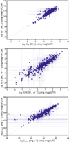 |
Fig. A.1. Physical properties estimated obtained from the SED fitting, using different miniJPAS magnitudes as input. In all panel the 1:1 relation is the dashed line. |
All Tables
All Figures
|
Fig. 1. In color, the main filter coverage between UV and mid-IR. For our SED fitting we have a total of 68 filters (colors). The five filters shown in grayscale on the background are the second option in case the main does not have an observation on the target. |
| In the text | |
|
Fig. 2. Sky map of the X-ray sources on and around the miniJPAS footprint (red box). Each dot represents an X-ray source in our compiled X-ray catalog, color-coded to show its original catalog. The size of the dots is proportional to their total X-ray flux measured in 0.5−10 keV. |
| In the text | |
|
Fig. 3. Hardness ratio as a function of redshift for Chandra sources in our sample (dots). The solid lines show the value of the corresponding column density, NH, for a fixed Γ = 1.4. The color of each source corresponds to the assigned NH (values in cm−2). |
| In the text | |
|
Fig. 4. Intrinsic X-ray fluxes as inferred after the NH correction vs. measured fluxes in the soft (0.5−2 keV, upper panel) and hard (2−10 keV, lower panel) bands. |
| In the text | |
|
Fig. 5. Distributions of spectroscopic redshifts (upper panel), intrinsic column density NH (middle panel), and hard X-ray luminosity (lower panel) for all sources in the EGS sample (green) and our final sample with miniJPAS detection and good photometry used in this work (red). |
| In the text | |
|
Fig. 6. Histograms of reduced χ2 for the SED fitting performed using two different sets of magnitudes extracted from miniJPAS catalogs, AUTO and PSFCOR (see Sect. 3.3). |
| In the text | |
|
Fig. 7. Criteria used to exclude the sources with unreliable physical parameters. The bayesian values for M⋆ (upper panel), SFR (middle panel), and LAGN (lower panel) are plotted against the ratio of best values over Bayesian. The distribution is centered at 1. The solid vertical lines mark the limits of 0.1 and 10 adopted in this work (see Sect. 3.3 for details). The different colors show the parameters and ratios obtained assuming different magnitudes as input. The number of sources between and outside the limits is reported in the lower part of the plots. |
| In the text | |
|
Fig. 8. Examples of SED fitting using CIGALE and their residuals. Pink circles show the photometry for each band used. Green triangles are upper limits. The black dashed line is the composite model, and the color lines are the individual components of the composite model. Left: full range of wavelengths, from X-ray to IR. Right: close up on optical miniJPAS J-spectrum. |
| In the text | |
|
Fig. 9. Examples of spectral fitting using PyQSOFit, and their residuals. On gray the spectra observed, at rest-frame wavelength. Continuum was fit as a polynomial, showed in orange. On cyan, the Fe emission. On blue, the emission lines fitted in the process to obtain FWHM of the BLR. |
| In the text | |
|
Fig. 10. Upper panel: comparison between our estimation of the black hole masses and the ones estimated by Rakshit et al. (2020) for the 88 sources in common. Bottom panel: histogram of the logarithmic difference of the BH masses. |
| In the text | |
|
Fig. 11. Histograms of the physical parameters estimated with the SED fitting (M⋆, LAGN and SFR). In red is the full sample while in green is the subsample with an estimation of MBH using the corresponding spectra. |
| In the text | |
|
Fig. 12. Distribution of accretion rates derived in this work. Upper panel: histogram of Eddington accretion rate (λEdd) for the sources with measured MBH. Middle panel: histogram of the specific accretion rate (λsBHAR, typically used as proxy of λEdd), for both the sample with measured BH masses and the full miniJPAS sample. A difference in the shape of distributions can be seen for the subsample with measured BH masses by comparing the green histograms in the upper and middle panels. Lower panel: plot of the relation between λsBHAR − λEdd. While they are defined to be equal, we found a poor correlation value and a systematic shift from the 1:1 relation in their linear regression (plotted as gray with 1-σ uncertainties in pink). |
| In the text | |
|
Fig. 13. Upper panel: accretion rate depending on LAGN. The solid line is the typical accretion rate assuming a linear dependence with LAGN, and it is equal for our sources with λ > λcrit. For the rest of the sources, the dispersion comes from the dependence with MBH, which is color-coded. Lower panel: histogram of the estimated BH accretion rates. |
| In the text | |
|
Fig. 14. Upper left panel: the observed MBH − M⋆ relation for all the 113 sources in our sample, at the observed redshift. Green solid dots are the value of masses for each source, with associated uncertainties, while contours are the distribution of these dots. In all panels, we show the expected local MBH − M⋆ scaling relations: in turquoise the 0.002 M⋆ from Marconi & Hunt (2003); in green the relation from Savorgnan et al. (2016) with uncertanties at 1-σ; in purple the unbiased version from Shankar et al. (2016) with uncertanties; and in brown the parametrization by Georgakakis et al. (2021). The other three panels show the forward modeling of our sources to z = 0 using different methods. Upper right panel: the most basic model, with constant rates (Scenario 1). Lower left panel: the model with a variable rate following the SFH (Scenario 2). Lower right panel: the model with a variable rate following the SFH and the energy limit for the black hole accretion (Scenario 3). See Sect. 6 for details. We also show the number of sources and the Pearson correlation value on each bottom right corner. |
| In the text | |
|
Fig. A.1. Physical properties estimated obtained from the SED fitting, using different miniJPAS magnitudes as input. In all panel the 1:1 relation is the dashed line. |
| In the text | |
Current usage metrics show cumulative count of Article Views (full-text article views including HTML views, PDF and ePub downloads, according to the available data) and Abstracts Views on Vision4Press platform.
Data correspond to usage on the plateform after 2015. The current usage metrics is available 48-96 hours after online publication and is updated daily on week days.
Initial download of the metrics may take a while.