| Issue |
A&A
Volume 672, April 2023
|
|
|---|---|---|
| Article Number | A46 | |
| Number of page(s) | 17 | |
| Section | Galactic structure, stellar clusters and populations | |
| DOI | https://doi.org/10.1051/0004-6361/202244766 | |
| Published online | 27 March 2023 | |
The Gaia-ESO Survey: Chemical evolution of Mg and Al in the Milky Way with machine learning⋆
1
Institute of Theoretical Physics and Astronomy, Vilnius University, Saulėtekio Av. 3, 10257 Vilnius, Lithuania
e-mail: markus.ambrosch@ff.vu.lt
2
Max Planck Institute for Astronomy, Königstuhl 17, 69117 Heidelberg, Germany
3
Leibniz-Institut für Astrophysik Potsdam (AIP), An der Sternwarte 16, 14482 Potsdam, Germany
4
Institut für Physik und Astronomie, Universität Potsdam, Karl-Liebknecht-Str. 24/25, 14476 Potsdam, Germany
5
Institute of Astronomy, University of Cambridge, Madingley Road, Cambridge CB3 0HA, UK
6
INAF – Osservatorio Astrofisico di Arcetri, Largo E. Fermi 5, 50125 Florence, Italy
7
Lund Observatory, Division of Astrophysics, Department of Physics, Lund University, Box 43 22100 Lund, Sweden
8
European Southern Observatory, Karl Schwarzschild-Straße 2, 85748 Garching bei München, Germany
9
Instituto de Física y Astronomía, Facultad de Ciencias, Universidad de Valparaíso, Av. Gran Bretaña 1111, Valparaíso, Chile
10
Niels Bohr International Academy, Niels Bohr Institute, University of Copenhagen Blegdamsvej 17, 2100 Copenhagen, Denmark
11
Nicolaus Copernicus Astronomical Center, Polish Academy of Sciences, ul. Bartycka 18, 00-716 Warsaw, Poland
12
INAF – Padova Observatory, Vicolo dell’Osservatorio 5, 35122 Padova, Italy
13
Núcleo de Astronomía, Universidad Diego Portales, Ejército 441, Santiago, Chile
14
Departmento de Astrofísica, Centro de Astrobiología (CSIC-INTA), ESAC Campus, Camino Bajo del Castillo s/n, 28692 Villanueva de la Canada, Spain
Received:
18
August
2022
Accepted:
25
January
2023
Context. To take full advantage of upcoming large-scale spectroscopic surveys, it will be necessary to parameterize millions of stellar spectra in an efficient way. Machine learning methods, especially convolutional neural networks (CNNs), will be among the main tools geared at achieving this task.
Aims. We aim to prepare the groundwork for machine learning techniques for the next generation of spectroscopic surveys, such as 4MOST and WEAVE. Our goal is to show that CNNs can predict accurate stellar labels from relevant spectral features in a physically meaningful way. The predicted labels can be used to investigate properties of the Milky Way galaxy.
Methods. We built a neural network and trained it on GIRAFFE spectra with their associated stellar labels from the sixth internal Gaia-ESO data release. Our network architecture contains several convolutional layers that allow the network to identify absorption features in the input spectra. The internal uncertainty was estimated from multiple network models. We used the t-distributed stochastic neighbor embedding tool to remove bad spectra from our training sample.
Results. Our neural network is able to predict the atmospheric parameters Teff and log(g) as well as the chemical abundances [Mg/Fe], [Al/Fe], and [Fe/H] for 36 904 stellar spectra. The training precision is 37 K for Teff, 0.06 dex for log(g), 0.05 dex for [Mg/Fe], 0.08 dex for [Al/Fe], and 0.04 dex for [Fe/H]. Network gradients reveal that the network is inferring the labels in a physically meaningful way from spectral features. We validated our methodology using benchmark stars and recovered the properties of different stellar populations in the Milky Way galaxy.
Conclusions. Such a study provides very good insights into the application of machine learning for the analysis of large-scale spectroscopic surveys, such as WEAVE and 4MOST Milky Way disk and bulge low- and high-resolution (4MIDABLE-LR and -HR). The community will have to put substantial efforts into building proactive training sets for machine learning methods to minimize any possible systematics.
Key words: Galaxy: abundances / Galaxy: stellar content / stars: abundances / techniques: spectroscopic / methods: data analysis
© The Authors 2023
 Open Access article, published by EDP Sciences, under the terms of the Creative Commons Attribution License (https://creativecommons.org/licenses/by/4.0), which permits unrestricted use, distribution, and reproduction in any medium, provided the original work is properly cited.
This article is published in open access under the Subscribe to Open model. Subscribe to A&A to support open access publication.
1. Introduction
The use of machine learning in the exploration of big data sets in astronomy was predicted over three decades ago (Rosenthal 1988), however, the high computational costs of this method have delayed its advancement. Some of the first applications of neural networks, a subfield of machine learning, include the automatic detection of sources in astronomical images (SExtractor, Bertin & Arnouts 1996), the morphological classification of galaxies (Lahav et al. 1996), and the classification of stellar spectra (Bailer-Jones 1997). In recent years, the increasing power of modern computer systems and the possibilities of cloud computing have led to a growing popularity of machine learning methods. Powerful open-source libraries such as TensorFlow (Abadi et al. 2015) and PyTorch (Paszke et al. 2019) for Python programming offer easy-to-use frameworks for building and training various types of neural networks.
Spectroscopic surveys provide insights into the evolution of individual stars, of large-scale structures such as globular clusters, and of the Milky Way galaxy as a whole. Upcoming projects, for example, the William Herschel Telescope Enhanced Area Velocity Explorer (WEAVE, Dalton et al. 2018) and the 4-m Multi-Object Spectroscopic Telescope (4MOST, de Jong et al. 2019) will carry out observations of millions of stars. Efficient automatic tools will be needed to analyze the large number of spectra that such surveys will deliver.
To determine the atmospheric parameters and chemical composition of stars, classical spectroscopic methods either measure equivalent widths of absorption lines or compare observed spectra to synthetic spectra. These synthetic spectra can be generated on the fly or make up part of a precomputed spectral grid. Jofré et al. (2019) provide an overview over classical spectral analysis methods in the context of large spectroscopic surveys.
Convolutional neural networks (CNNs) have recently been used to simultaneously infer multiple stellar labels (i.e., atmospheric parameters and chemical abundances) from stellar spectra. Every CNN contains convolutional layers that enable the network to identify extended features in the input data. In stellar spectra these features are absorption lines and continuum points. In 2D images, such features could be eyes in a face or star clusters in a spiral galaxy (Bialopetravičius & Narbutis 2020). Neural network methods are purely data-driven and therefore require no input of any physical laws or models. Instead, during a training phase, the network learns to associate the strength of spectral features with the values of the stellar labels. This requires a training set of spectra with pre-determined labels, from which the network can learn. Training sets for spectral analysis typically contain several thousand stellar spectra with high quality labels. Current spectral surveys, which provide ∼105 spectra with labels, are an ideal testing ground for the CNN approach to spectral parameterization.
The main benefit of using machine learning for spectra parameterization is computation speed. While classical methods typically take several minutes to determine parameters and abundances from a single spectrum, a trained CNN can parameterize several 104 spectra in the same amount of time. This speed is crucial to fully utilize the capabilities of the upcoming spectra surveys. For instance, 4MOST will observe ≈25 000 stars per night, with the goal of measuring up to 15 abundances per star. Machine learning will offer a way to manage such large amounts of data every day.
Examples of stellar parameterization using CNNs can be found in several recent studies. Fabbro et al. (2018) have developed StarNet, a CNN that is able to infer the stellar atmospheric parameters directly from observed spectra in the APO Galactic Evolution Experiment (APOGEE, Majewski et al. 2017). A grid of synthetic spectra was used to train and test StarNet. Purely observational data from APOGEE DR14 were used by Leung & Bovy (2019) to train their astroNN convolutional network. To mimic the methods of standard spectroscopic analysis, astroNN is designed to use the whole spectrum when predicting atmospheric parameters but is limited to individual spectral features for the prediction of chemical abundances. Guiglion et al. (2020) trained their CNN on medium-resolution stellar spectra from the RAdial Velocity Experiment (RAVE, Steinmetz et al. 2020) together with stellar labels that were derived from high-resolution APOGEE DR16 spectra. They also added absolute magnitudes and extinction corrections for their sample stars as inputs for the network. This information allowed their CNN to put additional constraints on its predictions of the effective temperature and surface gravity.
In this work, we propose to test a CNN approach in the context of the Gaia-ESO survey (GES, Gilmore et al. 2012; Randich & Gilmore 2013). We use GIRAFFE spectra with labels from the sixth internal data release. The GES survey is designed to complement the astrometric data from the Gaia space observatory (Gaia Collaboration 2016). The goal of the present project is to prepare the groundwork for machine learning techniques for the next generation of spectroscopic surveys, such as 4MOST and WEAVE. This paper goes together with Nepal et al. (2023) who focus on the chemical evolution of lithium with CNNs from GES GIRAFFE HR15N spectra.
This paper is organized as follows: In Sect. 2, we present the data that we used to train and test our CNN. Section 3 describes the architecture of our network and explains the details of the training process. The results of the training and the network predictions for the observed set are presented in Sect. 4. In Sect. 5, we validate our results by investigating the CNN predictions for a number of benchmark stars. For the further validation, we use our results to recover several properties of the Milky Way galaxy.
2. Data
2.1. Data preparation
Our data set consists of the spectra, their associated stellar parameters, and abundances from the GES iDR6 data set. In the Gaia-ESO survey, atmospheric parameters and chemical abundances are determined by multiple nodes that apply different codes and methodologies to the same spectra. A summary of the determination of atmospheric parameters from the GIRAFFE spectra is given in Recio-Blanco et al. (2014). Further information about the determination of chemical abundances can be found in Mikolaitis et al. (2014). The spectra were taken with the GIRAFFE spectrograph that covers the visible wavelength range of 370−900 nm. Several setups divide the whole GIRAFFE spectral range into smaller parts. For this study, we chose the HR10 (533.9−561.9 nm, R = 19 800) and HR21 (848.4−900.1 nm, R = 16 200) setups because they cover important Mg and Al absorption features.
For our analysis, we used normalized 1D spectra from the GES archive. We removed bad pixels and cosmic ray spikes where necessary. To do so, we first calculated the median of all spectrum flux values. We then identified cosmic ray spikes by finding all pixels with flux values that exceeded this median flux by five sigma. The spikes were removed by setting their flux value to be equal to the spectrum median flux. Pixels with zero flux values were also set to the median flux. Afterward, we corrected the spectra for redshift based on the radial velocity provided by GES. To reduce the number of pixels per spectrum and therefore the computational cost of the further analysis, we rebinned the spectra to larger wavelength intervals per pixel. The HR10 spectra were resampled to 0.06 Å per pixel and the HR21 spectra to 0.1 Å per pixel. The original bin size for both setups is 0.05 Å per pixel. After rebinning, the spectra were truncated at the ends to ensure that all spectra from one setup share the exactly same wavelength range. Eventually, we combined the HR10 and HR21 spectra to create one input spectrum per star for our network. The combined spectra are composed of 8669 pixels each and cover the wavelength ranges from 5350−5600 Å and 8480−8930 Å.
To build our training set, we performed several quality checks to ensure that our network would be trained on high-quality data. Spectra of a signal-to-noise ratio (S/N) < 30 and large errors in atmospheric parameters and elemental abundances (eTeff > 200 K, elog(g) > 0.3 dex, eA(element) > 0.2 dex) were discarded, as well as spectra that were marked with the TECH or PECULI flags or have rotation velocities > 20 km s−1. We also removed spectra that showed a difference larger than 0.2 dex between the provided metallicity [Fe/H] (as a stellar atmospheric parameter) and the Fe I elemental abundance. Similar to Guiglion et al. (2020), we tested the inclusion of lower S/N spectra into our training set. This increases the number of training spectra considerably, but the training performance gets worse and the overall prediction quality of our network decreases. While overly noisy spectra worsen the performance of our network, a moderate degree of noise is beneficial because it plays an important role in the regularization of the training process (Bishop 1995, particularly Sect. 9.3 therein). To exclude very noisy spectra, while still utilizing the regulatory effect of noise in the training data, we set the lower S/N limit for our training set to 30.
We further examined the remaining spectra to find possible outliers and incorrect measurements. To investigate the similarity between all the spectra, a t-distributed stochastic neighbor embedding (t-SNE) analysis was employed. The t-SNE analysis is a popular technique to visualize the internal relationships and similarities in high dimensional data sets by giving each data point a location in a two- or three-dimensional similarity map (van der Maaten & Hinton 2008). In our case, the data points are the individual spectra and the data set is n-dimensional, where n is the number of pixels in each spectrum. Figure 1 shows a two-dimensional similarity map for our combined spectra, obtained with the sklearn.manifold library for Python programming (Pedregosa et al. 2011). Every point in the map corresponds to one spectrum, and the distance between the individual points is determined by the similarity of the shapes of the individual spectra. There are two main branches in the map with several sub-structures. The two branches represent spectra from stars in two distinct populations: Main sequence stars with surface gravity log(g) ≳ 3.5 and stars in the giant branch with lower log(g) values. The different physical properties in stellar atmospheres are reflected in the shapes of their spectra, which in turn determine their locations on the t-SNE map. The connection between physical parameters and spectral features is what our CNN learns during the training phase. It is worth to mention that t-SNE on its own has also been used to classify spectra: Traven et al. (2017), for example, used t-SNE as a tool to separate GALAH spectra into different, physically distinct classes; Matijevič et al. (2017) used t-SNE to search for metal-poor stars in the RAVE survey.
 |
Fig. 1. t-SNE similarity map of our sample GIRAFFE spectra. The three panels show the same map, each color-coded with a different physical parameter. While the relative distance of points in the map indicate the degree of similarity of the corresponding spectra, their X and Y coordinates themselves have no physical meaning. The map in this figure has been computed with perplexity 30. For our data, perplexity values between 20 and 50 produce qualitatively identical results. |
We see several outlier-spectra in our Fig. 1. Upon inspection, these spectra show signs of emission lines, have distorted absorption features or have suffered from failed cosmic removal or wrong normalization. We excluded these outliers from the further analysis. For the analysis of future surveys such as WEAVE and 4MIDABLE-HR surveys, including emission line stars will be a necessity, as we expect many young stars to be observed. We note that the initialization of our t-SNE application includes an element of randomness, which results in slightly different shapes of the map after every run. The map will also look different for different sets of spectra. However, in all our t-SNE runs, the outlier spectra were clearly identifiable.
Every training spectrum has a set of associated stellar labels. In our case these are the two atmospheric parameters Teff and log(g) and the chemical abundances [Mg/Fe], [Al/Fe], and [Fe/H]. In the GES iDR6 data set the elemental abundances are given as absolute abundance values A(Element). We calculated [Fe/H] and [Element/Fe] as follows: [Fe/H] = A(Fe)star − A(Fe)⊙ and [Element/Fe] = A(Element)star − A(Element)⊙ − [Fe/H]. The absolute solar abundances were taken from Grevesse et al. (2007), consistently with GES spectral analysis strategy. The decision to use these relative abundances instead of absolute abundances for the training of our network is justified in Sect. 4.4.
Magnesium and aluminum abundances are known to be sensitive to non-local thermodynamic equilibrium (NLTE) effects (Bergemann et al. 2017; Amarsi et al. 2020; Lind et al. 2022). These effects were not considered by GES during the parametrization of GIRAFFE spectra or during the homogenization (Hourihane et al., in prep.). For dwarfs, NLTE corrections are well below 0.05 dex for both Al and Mg, whereas for giants, they are in the range of ∼0.05 − 0.15 (Amarsi et al. 2020). Strong NLTE effects may then have some effects on the training labels, but quantifying such an effect is beyond the scope of the present paper.
After applying all the constraints mentioned above, we were left with 14 634 combined spectra with associated high-quality atmospheric parameters and elemental abundances. As explained in Sect. 3.2.1, these 14 634 spectra will be randomly split into a training set and a test set for the training of our CNN.
2.2. Parameter space of input labels
To assess the parameter space of our training set input labels, we show the Kiel diagram and abundance plots in Figs. 2 and 3. Effective temperatures range from Teff = 4000 − 6987 K, the surface gravity log(g) is between 1.08 and 4.87 dex and [Fe/H] spans a range of ∼2 dex, from −1.53 to 0.72 dex. The color-coding in Fig. 2 reveals the metallicity sequence in the giant-branch of the Kiel diagram.
 |
Fig. 2. Kiel diagram containing the 14 634 stars that will be used to train and test our neural network. The color-coding indicates the metallicity gradient in the giant branch stars. |
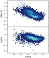 |
Fig. 3. Density plots of [Mg/Fe] vs. [Fe/H] (top panel) and [Al/Fe] vs. [Fe/H] (bottom panel) for the 14 696 stars in the training and test sets. Brighter colors indicate a higher density of data points (linear color scale). |
Figure 3 shows density maps of the [Mg/Fe] and [Al/Fe] distribution of our training set. The [Mg/Fe] values range from −0.25 to 0.80 dex, [Al/Fe] values have a large spread of almost 2 dex, from −0.95 to 1.00 dex. The Mg distribution reveals two distinct regions of enhanced density, separated by a narrow region of lower density. These two regions reflect the separation of Milky Way stars into a thin-disk (low [Mg/Fe]) and a thick-disk (enhanced [Mg/Fe]) population. Magnesium abundances are the best probe for this chemical separation between the thin- and thick-disk of our Galaxy (e.g. Fuhrmann 1998; Gratton et al. 2000). As expected, we did not observe this separation in the [Al/Fe] plot. Our training set is dominated by nearby stars, due to the S/N cut and other quality criteria that we applied to the entire GES iDR6 data set. Therefore, our data does not cover some of the Milky Way properties that become apparent when investigating a larger volume of our galaxy. Queiroz et al. (2020), for example, found two detached [Al/Fe] sequences for stars close to the galactic center (RGal < 2 kpc) in their sample of APOGEE stars. At low [Fe/H], several groups of stars can be observed in both the Mg and Al plots. The stars in these patches belong to different globular clusters. In the [Al/Fe] plot, the scatter of Al abundances in the globular clusters is considerably higher than the scatter of Mg at equal metallicities. This large spread of Al abundances, especially in globular clusters at low metallicities, has already been observed in earlier GES releases (Fig. 4 in Pancino et al. 2017a) and indicates the existence of multiple stellar populations within the clusters.
2.3. Observed sets
In addition to the training and test sets, we constructed an “observed” set. This set is used to test the performance of our CNN on spectra that were not used in the training process. In this way, we can mimic the application of our CNN method to newly observed spectra, which have not yet been analyzed spectroscopically. The full observed set therefore contains spectra without any applied quality constraints and spans wider S/N and label ranges than the training set. As we show in Sect. 4, our network is not able to accurately label spectra that are outside the training set limits. Because of this, we had to find a way to identify spectra that are similar to our training spectra, as the labels of these spectra are likely to fall into the training set limits. We already demonstrated in Sect. 2.1 that t-SNE is able to show the similarity between spectra. We therefore employed t-SNE to identify those spectra in the observed set whose labels are likely to be within the training set limits. A depiction of this method can be seen in Fig. 4. In the left panel, we show a t-SNE map that was calculated for all spectra in our data set. After constructing the t-SNE projection, we identified the training spectra in the map. The middle panel shows those spectra in the observed set that cover the same area in the t-SNE map as the training spectra in the left panel. This was done by limiting the distance between training set data points and observed set data points in the t-SNE map. The observed spectra that are close to the training spectra in the map are similar to the training spectra. We call this set in the middle panel our “inner” observed set. Finally, the right panel shows those spectra that are not similar to the training spectra, and their distance from the training spectra in the map exceeds our chosen maximum distance. This set of spectra is our “outer” observed set, and we use it to test our network on spectra which are unlike the spectra in the training set. Because the labels for the observed set have already been determined by GES, we can quantify the effectivity of this t-SNE approach: About 20% of all observed spectra have GES labels outside the training set limits. The situation improves for our inner observed set, with 12% of its spectra labels falling outside the training limits. When we additionally require the S/N of the inner set to be ≥30 (to match the S/N range of the training set), less than 10% of these high S/N inner set spectra have labels exceeding the training limits. In a situation where the labels of an observed spectrum are not yet known, we therefore recommend validating if the spectrum is similar to the training set spectra.
 |
Fig. 4. t-SNE maps of different subsets of spectra. Left panel: all spectra in our GIRAFFE data set (dark blue), containing the training set spectra (green). Extreme outlier spectra have been removed. Middle panel: “inner” observed set, defined as the subset of observed spectra that cover the same area in the t-SNE map as the training set spectra. Right panel: spectra in the observed set that do not cover the same area in the map as the training set. This is our “outer” observed set. |
Our full observed set contains 22 270 spectra, with a minimum S/N of 10 and including spectra with different shapes than those in the training set. The outer observed set contains 3877 spectra. The inner observed set then consists of the remaining 18 393 spectra which are covering the same area in the t-SNE map as the training spectra. Of the inner observed spectra, 4916 have S/N ≥ 30.
3. Network architecture and training
A CNN acts as a function with many free parameters. In our case, this function takes stellar spectra as an input and outputs the associated atmospheric parameters and abundances. The network architecture then describes the shape of this neural network function. The goal of the training process is to find the optimal values of the free CNN parameters to accurately parameterize the input stellar spectra. In the following subsections, we describe how a neural network can “learn” how to accurately parameterize stellar spectra. Our CNN was built and trained in a Python programming environment with the open-source deep-learning library Keras (Chollet et al. 2015) using the TensorFlow back-end (Abadi et al. 2015). The following subsections give an overview of the key concepts of network architecture and training that form the basis of this study. There are numerous textbook sources, articles, and online resources that provide more detailed information, both from a theoretical and practical point of view, such as Roberts et al. (2022), Giancarlo & Md. Rezaul (2018), and Alzubaidi et al. (2021).
3.1. Network architecture
The different parts of a neural network architecture, namely, the “layers”, serve different purposes in the process of parameterizing stellar spectra. Our neural network consists of two main types of layers: Convolution layers that identify features and patterns in the input spectra and dense layers, which associate those spectral features to the output stellar parameters. Finding the optimal network architecture for a given task requires some experimentation. We built and tested several networks with different hyper-parameters (number and size of the convolution and dense layers, type of weight initialization, dropout rate, etc.). We did this until we arrived at an architecture that provided the best trade-off between computation time, reached precision, and convergence for our sample spectra. A visualization of the network architecture, which produced the lowest final loss (see Sect. 3.2), can be seen in Fig. 5. We adopted this architecture for the rest of the current study.
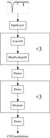 |
Fig. 5. Architecture of our CNN. The input layer reads in the flux information of the stellar spectra. It is followed by three pairs of convolution and max-pooling layers. The filter outputs from the third convolution and max-pooling pair are then flattened to serve as inputs for the dense layers. Three dense layers (with a dropout layer after each) interpret the spectral features, found by the convolution layers, into output labels. The outputs from a last dense layer are the values of our five stellar labels (atmospheric parameters and elemental abundances). |
3.1.1. Convolution layers
To identify the spectral features that are correlated with the stellar labels, our CNN is composed of convolution layers. These layers convolve the input spectra with a number of 1D filters. The filters move across the input spectra and produce feature maps, which are the results of the spectrum-filter convolutions. While the length and number of filters is fixed, the purpose of each filter is learned during the training phase. The neural network learns how to adjust the filter values to achieve the best label predictions. Multiple convolution layers with multiple filters each can be put in sequence in a neural network architecture. Filters in one convolution layer then extract features in the feature maps that were produced by the previous convolution layer. Our CNN has three convolution layers with an increasing number of filters in each layer.
3.1.2. Dense layers
In order to build a high-dimensional complex function between the feature maps from the last convolution layer and the labels, so-called dense layers are necessary. Each dense layer consists of a fixed number of artificial neurons. An artificial neuron receives inputs from a previous layer, multiplies every input with its associated weight and then passes the result to the neurons of the next dense layer. In this way, every neuron in one dense layer is connected to all neurons of the previous layer and to all neurons of the following layer (this is the reason why dense layers are also called “fully connected” layers). The last layer in a CNN is a dense layer where the number of neurons is equal to the number of labels that the network is designed to predict (in our case 5).
3.1.3. Activation function
The relations between spectral features and physical stellar labels are non-linear. To reflect this non-linearity in our network training process, activation functions are used. Activation functions transform the output of the convolution filters and the artificial neurons before they are passed on to the next layer. In some recent machine learning applications, the “Leaky ReLU” activation function is most frequently used. It leaves positive and zero output values unchanged, while multiplying negative outputs with a small positive value – or, as per the mathematical notation (Maas et al. 2013):
where x is a filter or neuron output value before it is passed to the next layer. For our network, we adopted a Leaky ReLU activation function with a = 0.3 for all layers.
3.1.4. Max-pooling and dropout
Overfitting occurs when the network is very accurate in predicting the labels of the training set, but shows a poor performance when predicting labels for the test set or an external observed set. In this case, the network is not generalizing well for inputs outside the training data. This is often the case when the network architecture is complex and the number of weights and biases is too large. In this context, max-pooling and dropout are popular regularization devices used to prevent overfitting during the training of a CNN.
Max-pooling helps to prevent overfitting by reducing the complexity of the feature maps that are produced by the convolution layers. This is achieved by keeping only the highest value within a defined interval in every feature map. In this way, the less important pixels of a feature map are discarded and the network is able to focus on pixels that show a strong response to the convolution filters.
Applying dropout after a dense layer randomly deactivates the output of a fraction of the layer neurons (these neurons are “dropped”). The weights associated with dropped neurons are therefore not updated for one training epoch (one passage of the entire training set through the network; see Sect. 3.2.2). After every epoch, all neurons are reactivated and a new collection of neurons is dropped for the next epoch. As a consequence, the network architecture changes slightly after every epoch during the training. This prevents the network from relying too much on individual parts of the architecture and therefore individual features in the input spectrum. In this way, the network is forced to learn from the whole spectrum, which leads to a good generalization for different input spectra.
3.2. Network training
When the network architecture is designed, the values of the convolution filter cells and the weights and biases in the dense layers are unknown. During the training phase, these values are “learned” by the neural network. Training means to repeatedly pass many spectra with known labels (training set) through the network and to compare the output of the network to the known input labels of the training set. At the start of the training phase, the filter values, weights and biases are initialized randomly. Therefore, the predictions of the untrained network will differ strongly from the labels of the input spectra. The difference between the network predictions for the labels and their known values from the input is called “loss” and it is calculated with a loss-function. The loss-function calculates the overall difference between input and output values across all labels. Therefore, the loss is a measure of the overall accuracy of the network predictions. An optimization algorithm is used to slightly change the weights and biases in the network in such a way that, when the training sample is passed through the network again, the loss will be slightly smaller than in the first iteration. Over the course of many iterations of passing the training spectra through the network, calculating the loss and updating the weights and biases for optimization, the loss steadily decreases and the network predictions get more precise (Figs. 6 and 7). In the following subsections, we explain in detail the key concepts involved in the training of our neural network.
 |
Fig. 6. Evolution of the prediction-based Kiel diagram during the network training. The far-left panel shows the Kiel diagram based on the GES input values of Teff and log(g). Succeeding panels show the Kiel diagram based on network predictions after 1, 10, and 150 training epochs. The color-coding, indicating the [Fe/H] values of each data point, is on the same scale as in Fig. 2. |
 |
Fig. 7. Evolution of the training and test losses during the network training phase. The loss of the test set is closely following the training loss. The small difference between training and test sets at the end of the training phase shows that the network is not overfitting. |
3.2.1. Training set and test set
Training relies on many stellar spectra (several thousand) with their associated stellar labels. In our case, the labels are previously determined stellar atmospheric parameters and chemical abundances (see Sect. 2). The available data are split randomly into a training set that is used to train the network and a test set. During training, the test set is passed through the network as often as the training set, but it is not used in the optimization calculations that update the weights and biases. Instead, the test set is used to monitor the performance of the network on data that it was not trained on. The loss calculated from the label predictions for the test set is used to determine when to stop the training: If the test loss does not increase any more over a specified number of training iterations, the weights and biases are assumed to have reached their optimal values for the given network architecture and the training ends. Comparing the performance of the network on the training and test sets also helps to determine if the network is overfitting. We found that assigning 40% of our available data to the test set yields the best training results for our application. That means that of our 14 696 spectra, 8817 spectra are assigned to the training set and 5879 to the test set. Training and test spectra are chosen randomly before the training and it is assured that their labels cover the same parameter space.
3.2.2. Epochs and batches
One iteration of passing the entire training set through the network is called an epoch. The number of epochs that are necessary to train a network to achieve good results depends on the model architecture.
In one epoch, the training data that is passed through the network is divided into equally sized batches. For example, for a training set of 6400 spectra and a batch size of 64, 100 batches pass through the network in one epoch. After every batch that passes through the network, the weights and biases are updated based on the current loss-function in an attempt to decrease the loss after the next batch. This means that in the above example the weights and biases are updated 100 times before the training set has fully passed through the network. This speeds up the overall training because less computer memory is required to process the smaller number of spectra for one update. Using batches can also help to prevent overfitting. The training spectra are shuffled and assigned to new batches after every epoch.
4. Training results
We performed ten training runs, which resulted in ten slightly different CNN models. The results of the training runs vary slightly because the weights and biases of the network are initialized randomly before every run (the network architecture remains the same). In addition, the assignment of spectra to batches for the training also happens randomly. The training and test sets remained unchanged for each of the ten training runs. We checked the label distributions for both the training and test set and found that both span the same label ranges and are equally distributed. They also span the same area in the t-SNE map in Fig. 4. We therefore do not expect that keeping the training and test sets constant will add any large uncertainties or training biases.
On average, one training run lasted for 159 epochs and took ∼45 min to complete1. We removed the two CNN models with the largest remaining test losses at the end of their training phase. The remaining eight CNN models were then used to predict the labels for the spectra in the training, test, and observed sets. The label prediction was very fast: the parameterization of the ∼37 000 spectra in our data set took less than 20 s per CNN model. The averages of the eight sets of labels are reported here as our results.
4.1. Training and test sets
In Fig. 8, we show a direct comparison between the input GES measurements and the CNN predictions for the training and test sets. There is a good agreement between the GES measurements and CNN predictions across all labels and for the two sets. Both the CNN predictions for the training set and test set show the same offset (if any) and a small dispersion around the 1:1 relation. This indicates that the network performs well on spectra which it was not directly trained on and does not overfit. The dispersion around the 1:1 relation is uniform across most of the value ranges of all five labels. We use the dispersion of the training set as a measure for the training precision of our network: The training precision is 37 K for Teff, 0.06 dex for log(g), 0.05 dex for [Mg/Fe], 0.08 dex for [Al/Fe], and 0.04 dex for [Fe/H]. However, our CNN does not accurately reproduce the highest and lowest GES measurements. This is especially apparent in the case of [Al/Fe], where the CNN predictions overestimate the lowest [Al/Fe] measurements by ∼0.5 dex, while the highest values are underestimated by approximately the same amount. We explain this behavior by noting that only a few spectra with these extreme measurements were available for the network training. The CNN therefore predicts more moderate labels for these spectra.
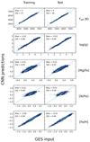 |
Fig. 8. One-to-one comparison of labels from GES iDR6 and the values predicted by our CNN. The two columns show results for the training and test sets. Each row contains the results for a different label. In every panel, the horizontal axis stands for the GES input labels, the vertical axis represents the labels predicted by our CNN. Brighter colors indicate a higher density of data points (linear color scale). The average bias and the standard deviation (scatter) of the results around the 1:1 relation are given in every panel. Solid diagonal lines indicate the 1:1 relation. |
4.2. Observed sets
To evaluate the ability of our network to parameterize new spectra that have not been involved in the training process at all, we compare the GES input labels to the CNN predictions for three different observed sets. The definitions of our inner and outer observed sets are given in Sect. 2.3. The left panel of Fig. 9 shows the GES input to CNN output comparison for the inner observed set spectra with S/N ≥ 30. In this subset, 90% of the GES labels lie within the training limits. Most of the remaining 10% of spectra are outside the [Mg/Fe] and [Al/Fe] limits. The reason for this lies in the way how we find our inner observed set. This set contains only stars that occupy the same area in a t-SNE map as the training spectra (Fig. 4). The shape of a spectrum, and therefore its position in the t-SNE map, depends strongly on the labels Teff, log(g), and [Fe/H], while changes in [Al/Fe] only have a small effect on the overall spectrum. The same is true for [Mg/Fe], but to a lesser extent. This is because there are more Mg absorption lines than Al lines in our sample spectra (Heiter et al. 2021). The accuracy of the network predictions stars to degrade with the low S/N inner observed set (middle panel of Fig. 9). This set contains spectra that are similar to the training spectra, but have lower S/N (we recall here that the minimum S/N of the training spectra is 30). The low-resolution inner set contains more spectra that are outside the training limits. It is clear that our CNN is not able to accurately parameterize spectra whose GES labels lie outside the training set range. The right panel shows the results for the outer observed set. Network predictions for this set are increasingly inaccurate, even for spectra inside the training set limits. The difference between GES input and CNN output for the outer observed set is most prominent in [Al/Fe] and [Fe/H], where extremely low and high GES labels are not accurately predicted by our network.
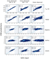 |
Fig. 9. One-to-one comparison of labels from GES iDR6 and the values predicted by our CNN. The three columns show results for the inner observed set in two different S/N ranges, and for the outer observed set. Each row contains the results for a different label. In every panel, the horizontal axis stands for the GES input labels, the vertical axis represents the labels predicted by our CNN. Brighter colors indicate a higher density of data points (linear color scale). The average bias and the standard deviation (scatter) of the results around the 1:1 relation are given in every panel. Solid diagonal lines indicate the 1:1 relation. Shaded areas indicate GES label values that are outside the training set limits. |
The comparison of the CNN predictions for the different observed sets highlight the importance of pre-selecting spectra that are likely to fall within the training set limits. Network predictions for spectra that are dissimilar to the training spectra or have lower S/N are likely to be inaccurate.
4.3. Estimation of internal precision
As described, the label predictions from our eight trained CNN models vary slightly. This variation can be used to estimate the internal precision of our methodology. We define the internal uncertainty of our results as the dispersion between the label predictions from the eight CNN models. In Fig. 10 we display the distribution of the internal uncertainty of our five labels relative to the predicted label values and to the spectra S/N. This analysis is done for both the inner observed set with S/N ≥ 30, the inner observed set with S/N < 30, and for the outer observed set. The boxplots show the spread and median of the uncertainties in S/N bins of 10, for the entire observed set. Where S/N ≥ 30, the uncertainties are small, with near constant mean and spread across all bins. Towards lower S/N, both the median uncertainty and the spread in the bins increase. The mean uncertainties of the label predictions for the high S/N inner observed set are small: 27 K for Teff, 0.04 for log(g), and 0.03 dex for [Mg/Fe], [Al/Fe], and [Fe/H] alike. The GES label errors for this set show little to no dependence on the absolute label value and S/N. Their mean values are 63 K for Teff, 0.15 for log(g), 0.22 dex for [Mg/Fe], 0.19 dex for [Al/Fe], and 0.18 dex for [Fe/H].
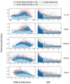 |
Fig. 10. Internal precision of our CNN results for the inner observed set with S/N ≥ 30 (light blue), with S/N < 30 (dark blue) and the outer observed set (red). The left panels show the internal precision relative to the absolute CNN label values, the right panels show the precision relative to the spectra S/N. The boxplots in the right panels show the median and spread of the uncertainties of the whole observed set, in S/N bins of width 10, starting at S/N = 10. |
The CNN predictions with large uncertainties for one label also show large uncertainties for all other labels, while precise predictions are precise across all five labels. The internal precision of our Teff and log(g) is highest where the training set density is highest. For Teff, this is the case between ∼4500 and 5775 K, for log(g) at ∼2.5 and 4.5 dex. Here, the uncertainties of the predictions for these two labels is lowest. Except for [Fe/H], the precision of the abundance predictions show no clear trends with the absolute label value. For [Fe/H], the uncertainty increases with lower [Fe/H] abundances. This is presumably due to the smaller number of stars in the metal-poor regime compared to the main bulk of the sample. Also, our CNN struggles to provide precise predictions due to the weak spectral features present in this [Fe/H] regime. We find that the uncertainties of the predictions for all five labels increase as the S/N of the spectra decreases.
The mean prediction uncertainties for the low S/N inner set and for the outer set are higher than for the high S/N inner observed set. Precision for these sets also show strong trends with the absolute label value, especially for Teff and [Fe/H].
We also tested how the uncertainty distributions change when we change the composition of the training and test sets for every training run. The resulting label uncertainties are similar to the uncertainties from our original approach. We leave the detailed investigation of the effect of varying train and test sets for a future work.
4.4. Learning from spectral features
The purpose of the convolution layers in our CNN is to find spectral features. These spectral features are then interpreted into the labels by the dense layers. This approach is also used by classical spectral classification methods, where individual spectral features are investigated to derive the stellar parameters. However, since machine learning is purely data-driven, the predictions of our CNN could merely be the result of our network learning correlations between labels in our data set. Individual elemental abundances for example are correlated with the iron abundance: stars with low iron generally show low abundances of other elements as well. Inferring stellar parameters from correlations such as these can lead to satisfying results for some spectra. However, stars with exotic chemical compositions (e.g., stars with a non-solar mixture of elements, such as old thick-disk stars) do not follow such trends and will not be parameterized well. We therefore want to show that our CNN is indeed able to identify spectral lines and to associate them with the right labels.
In order to visualize where our CNN is active for a given label, we computed sensitivity maps using GradientTape from TensorFlow. In general, CNN established a mapping between input spectra and output labels in a differentiable way, so CNN can be optimized using gradient descent. Using automatic differentiation, we can compute the gradients, ∂ Label/∂ λ, that is, the sensitivity of the CNN to each pixel for every label. A large absolute gradient value at a wavelength bin then means that the network is very sensitive to flux changes in that bin. In Fig. 11, we show the network gradients for our five labels across the whole wavelength range of the input spectra. The gradients are scattered randomly around zero for most of the wavelength range. It is only at certain wavelength bins that the network is sensitive to flux changes. Here, the gradients show individual, narrow spikes. This is especially apparent in the gradients for [Mg/Fe] and [Al/Fe] in the HR21 part of our input spectra. The [Mg/Fe] gradients show two clear spikes at 8736.0 and 8806.8 Å. These are the locations of two Mg I absorption lines. The largest spike in the [Al/Fe] gradients mark the location of the Al I double feature at ∼8773 Å. We therefore see that our network is able to identify absorption lines in the input spectra. The negative gradient values at these wavelengths means that if the flux at the absorption lines are low, the predicted abundance is high, and vice versa. This reflects the fact that stronger absorption features in spectra indicate higher elemental abundances in stellar atmospheres. The CNN label predictions are therefore directly based on the strength of the relevant absorption lines in the input spectra.
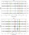 |
Fig. 11. Network gradients for our five labels as a function of wavelength (black). Top panel shows the gradients across the GIRAFFE setup HR10. Bottom panel shows the same for the HR21 setup. An average input spectrum is shown in gray as the top line in both panels. The locations of selected absorption lines of different elements are marked with vertical colored lines. The highlighted Mg and Al lines were used by GES for the determination of our input Mg and Al abundances. Their wavelengths are 5528.41, 8717.81, 8736.02, and 8806.756 Å for Mg and 5557.06, 8772.87, and 8773.90 Å for Al (Heiter et al. 2021). |
Our network does not only learn from the correlation between spectral features and stellar labels in individual stars, but also from correlations between labels across the whole training set. These data-wide correlations are of astrophysical origin, showing for example that stars with high iron abundance generally also have high abundances of other metals. To investigate how astrophysical correlations in the input data influence the network gradients, we trained our CNN with different combinations of input labels. We found that the gradients of a combination of Teff, log(g), and one or all of the abundances show no gradient correlations – meaning the CNN learns mainly from the spectral features. If the network is trained only with the highly correlated labels A(Mg), A(Al), and A(Fe), which are absolute abundances, the gradients for the three labels are almost identical (Fig. 12). In this case the CNN is still able to identify the locations of the Mg, Al and Fe absorption lines, but the network predictions for one element is also very sensitive to absorption lines of the other two elements. In addition, the quality of the CNN predictions starts to degrade, leading to larger differences between GES input labels and CNN predictions. This is because the network relied too much on the label correlations within the training set instead of the connection between spectral features and labels of individual spectra. For future surveys, we therefore recommend to carefully inspect the training data for strong correlations because they can influence the CNN performance.
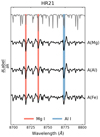 |
Fig. 12. CNN sensitivity maps when trained only on the highly correlated labels A(Mg), A(Al), and A(Fe). For clarity, this figure focuses on a wavelength range in the GIRAFFE HR21 setup that contains two Mg and one Al line. |
Further investigation of the gradient peaks gives interesting insights into the behavior of our CNN. Some spectral lines influence the network predictions for only one of the labels. An example in the HR10 setup is a Cr I line at ∼5410 Å, that corresponds to a peak in the gradient for Teff. Other lines have an effect on multiple, uncorrelated labels. For deriving Teff and log(g), our CNN is sensitive to the Ni I line in the red end of the HR10 setup. While this line coincides with the strongest peak in the log(g) gradient, only a minor peak is present in the Teff gradient. A Fe I line at ∼8805 Å is also important for both the Teff and log(g) predictions, but not for the [Fe/H], likely due to its blend with a Mg line. The infrared calcium triplet (the three most prominent absorption lines in the HR21 setup) does not have a significant influence on the network predictions for any of the labels, but the Ca II line beyond 8900 Å causes a very strong response of the Teff and [Fe/H] gradients. A deeper investigation of the CNN gradients could be done to search for complementary spectral features that could be used by standard spectroscopic pipelines, but this is beyond the scope of the present paper.
5. Validation of results
In this section, we validate our results in three ways. First, we compare our CNN results to the GES labels for a set of benchmark stars. Then we compare our log(g) predictions to CoRoT log(g) values that were derived using asteroseismology. In this way, we can validate, both with an internal and an external data set, the assumption that our CNN can accurately parameterize individual spectra. Finally, we investigate the label predictions for spectra from stars in different stellar populations to confirm that our results recover important Milky Way properties. Our validation covers the results from our whole sample of spectra, combining training, validation, and observed sets.
5.1. Benchmark stars
The GES iDR6 data set contains a number of benchmark stars with high quality spectra and precise stellar labels (Heiter et al. 2015). This benchmark set covers stars in different evolutionary stages with a wide range of stellar parameters and abundances suited for the verification and calibration of large data sets (Pancino et al. 2017b). Our data set contains 25 benchmark stars, including the Sun (see Fig. 13). As for the rest of our data set, the labels for the benchmark stars were determined spectroscopically by GES. We note that none of the benchmark stars are present in the training or test sample. Five of the benchmark stars are not part of the inner observed set, meaning that their spectra are different from the training set spectra. Four of them have the lowest [Fe/H] of all benchmark stars, while the fifth is the benchmark star with the highest [Fe/H] in our data set. The CNN predictions for these five stars do not match the GES input values well. The CNN predictions of the remaining 20 benchmark stars, which are part of the inner observed set, agree well with the GES values across all five labels. The largest differences occur for stars on the edges of the parameter space, where the network predicts more moderate values compared to the extreme GES values. An example is HD 49933, the benchmark star with the highest Teff, for which our network predicts ∼350 K less than what is reported by GES. This star remains one of the hottest in our benchmark set, even with this reduction in Teff. Despite the large difference in one label, the CNN predictions for the other labels of HD 49933 agree well with the GES measurements. The label-specific bias and scatter between GES and CNN labels for the benchmark stars in the inner observed set is comparable to the bias and scatter that we found for the training and test sets in Fig. 8.
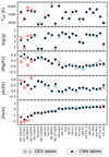 |
Fig. 13. Comparison of GES input labels with CNN predictions for the benchmark stars. The five red data points represent benchmark stars that are in the outer observed set. Blue data points are benchmark stars in the inner observed set and have S/N ≥ 30. Different data point sizes have no physical meaning and are for visualization purposes only. |
The CNN predicts similar label values for repeat spectra of our benchmark stars, often predicting identical labels for multiple repeats. The dispersions between repeated label predictions can be interpreted as the uncertainties of the CNN results. These CNN uncertainties are within the GES label uncertainties for the benchmark stars.
We conclude that our CNN is able to accurately predict multiple labels of individual stars, as long as their spectra are similar to the training set spectra. However, the most extreme CNN results should be used cautiously because they are likely to be underestimating high values and overestimating low values.
5.2. Comparison to asteroseismic surface gravities
Asteroseismology is an extremely powerful tool that provides accurate surface gravities, based on stellar oscillations. This method is massively used by spectroscopic surveys for validation or calibration purposes (RAVE, Valentini et al. 2017; APOGEE, Pinsonneault et al. 2018). Our aim here is to compare the log(g) values of our GES input data and our CNN results to GES-CoRoT log(g) values from Valentini et al. (2016). The Convection, Rotation and planetary Transits (CoRoT) mission was a space observatory dedicated to stellar seismology. Contrary to the labels of the benchmark stars, the asteroseismic surface gravities are not derived from stellar spectra. The CoRoT measurements therefore offer a good opportunity to validate our CNN predictions with a completely external data set. We show this comparison in Fig. 14. The one-to-one relation between GES log(g) values and asteroseismic CoRoT results shows no residual trend, with a low dispersion of 0.08 dex. The CNN log(g) values show also no residual trend compared to GES-CoRoT log(g) and a similarly small dispersion.
 |
Fig. 14. One-to-one comparison of input GES and output CNN labels with log(g) values derived using asteroseismology (Valentini et al. 2016). |
5.3. Globular clusters
Our data set covers stars that belong to a number of different globular clusters. We identified member stars of five separate clusters based on their position in the sky and their scatter in [Fe/H] and radial velocities that are reported in GES iDR6. The position of the cluster members in the [Mg/Fe] and [Al/Fe] plots is displayed in Fig. 15. The CNN predictions reproduce the grouping of cluster members in the plots, with a small spread of [Fe/H] within each cluster. However, the CNN predictions show a smaller scatter in [Element/Fe] compared to the GES values, especially for Al. This reduced scatter is a reflection of the results that we saw in Figs. 8 and 9, where the CNN predicts more moderate labels for spectra with extreme GES labels.
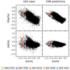 |
Fig. 15. [Mg/Fe] and [Al/Fe] vs. [Fe/H] plots for stars in the training, test, and observed sets. The panels on the left show the distributions of the GES iDR6 values, panels on the right are the predictions of the trained neural network. Cluster membership is indicated by differently colored data-points. |
Our CNN results recover the Mg-Al anti-correlation, which is used to investigate the chemical evolution of globular clusters (Pancino et al. 2017a). Figure 16 shows the Mg-Al anti-correlation in the clusters NGC 6752, NGC 6218, and NGC 1851. The average [Fe/H] values of these three clusters span a range of ∼0.5 dex. We see that the match between GES input and CNN output is improving with increasing cluster [Fe/H]. The cluster NGC 6752 contains stars with [Fe/H] values at the lower edge of the training set limit, where the density of training spectra is low. The density of the training set increases with [Fe/H], which leads to better CNN predictions for the cluster stars. Except for the star with the highest [Al/Fe], all CNN predictions for the NGC 6218 agree with the GES results within their reported uncertainties. For NGC 1851, which has the highest average [Fe/H] value among the clusters in our sample, we observe a good match between the Mg-Al anti-correlation as measured by GES and our predicted anti-correlation.
 |
Fig. 16. Mg-Al anti-correlation plots for three of our sample clusters with decreasing cluster metallicity. Colored data points show the labels predicted by the CNN, black points are the GES results. The colors for the different clusters is the same as in Fig. 15. Average uncertainties of the GES results are shown in the lower left corner. |
5.4. Thin- and thick-disk populations
As discussed in Sect. 2.2, [Mg/Fe] values can be used to separate the Milky Way stars into a thin-disk and a thick-disk population. We performed this separation based on our CNN results for the inner observed set with S/N ≥ 30 in combination with the test set. We also attempted to perform the separation for the combination of the low S/N inner observed set and outer observed set. The top panel of Fig. 17 shows the distribution of [Mg/Fe] versus [Fe/H] for the CNN predictions for the low S/N set plus the outer observed set. We can see that the stars are not separated into the two distinct thin- and thick-disk populations. The CNN predictions for both [Mg/Fe] and [Fe/H] are strongly clustered around the label averages and it is not possible to clearly separate the stars into the two populations. The bottom panels show the same plot for the inner observed set with S/N ≥ 30 plus the test set. Here, we can see the separation between the two disks: Thin-disk stars with [Mg/Fe] lower than ∼0.2 dex and thick-disk stars with enhanced [Mg/Fe]. To identify the thick- and thin-disk stars, we used the clustering algorithm HDBSCAN (Campello et al. 2013), which is implemented in the hdbscan library for Python programming. This algorithm assigns data points to different clusters, depending on the density of data points in a distribution. Two clusters are identified that correspond to the two stellar populations, as displayed in the bottom panel of Fig. 17. About 35% of the stars do not fall into any of the two clusters. Stars outside the two dense regions in the distribution are considered to be “noise” by the HDBSCAN algorithm and are not assigned to any cluster. In the literature, the chemical separation between thin and thick disk is often performed by splitting the distribution into several [Fe/H] bins and finding the [Mg/Fe] value in each bin where the density of stars is at a minimum (e.g. Adibekyan et al. 2011; Mikolaitis et al. 2014). Anders et al. (2018) use a sophisticated t-SNE approach to identify the different stellar populations. They include abundances measurements from 13 chemical elements to further dissect the thin and thick disk into additional subpopulations.
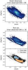 |
Fig. 17. Chemical separation between thin- and thick-disk stars. Top panel: density map of the [Mg/Fe] vs. [Fe/H] distribution of our CNN results for the low S/N inner + outer observed sets. Brighter colors indicate a higher density of data points (linear color scale). Bottom panels: same plot as in the top panel, but for the stars in the test and inner observed set with S/N ≥ 30. Thin and thick disk populations found by the HDBSCAN algorithm are shown at the bottom. The two populations correspond to the two dense regions in the panel above. |
To investigate the age distributions of the two populations, we used the isochrone fitting code Unified tool to estimate Distances, Ages and Masses (UniDAM). The UniDAM tool (Mints & Hekker 2017) follows a Bayesian approach of isochrone fitting. It compares stellar atmospheric parameters and absolute magnitudes from simulated PARSEC isochrones (Bressan et al. 2012) to the corresponding values in observed stars. All PARSEC isochrones also have stellar masses and ages associated with them. For the isochrone fitting we used the CNN predictions for the atmospheric parameters Teff and log(g) in combination with [Fe/H]. Magnitudes of our sample stars in the J, H, and K bands were taken from the 2MASS catalog (Skrutskie et al. 2006). In order for UniDAM to calculate the absolute magnitudes, it is also necessary to provide the parallax value for each sample star. We used the parallaxes from Gaia EDR3 (Gaia Collaboration 2021). We removed stars with negative parallaxes as well as stars with relative parallax errors > 0.2. To get the most precise age estimates, we only considered turn-off stars in this analysis. Turn-off stars in our thin and thick disk samples were selected by their position in the Kiel diagram. The resulting average age of the thin-disk stars is 8.7 Gyr, the average thick disk age is 9.7 Gyr. This age difference between the two populations has been found in numerous studies and by using several different age determination methods. Kilic et al. (2017), for example, found ages from 7.4−8.2 Gyr for the thin disk and 9.5−9.9 Gyr for the thick disk by analyzing luminosity functions of white dwarfs in the two disks. Using APOGEE spectra and precise age estimates based on asteroseismic constraints, Miglio et al. (2021) also showed that the chemically selected thick disk stars are old, with a mean age of ∼11 Gyr. We note that the detailed age distribution of thin and thick disk members is sensitive to several selection criteria such as metallicity, kinematic properties and the distance from the Milky Way center. A detailed investigation of the two stellar populations is out of the scope of this work.
We also investigated the kinematical properties of our thin and thick disk samples. Based on the current positions and velocities of the stars, we integrated their orbits for 5 Gyr in a theoretical Milky Way potential, using the Python-based galactic dynamics package galpy (Bovy 2015). For the integration we used the gravitational potential MWPotential2014, which combines bulge, disk, and halo potentials. Proper motions, sky coordinates, and parallaxes of our sample were taken from the Gaia EDR3. In Fig. 18, we show the trends of the orbital eccentricities relative to [Fe/H] for our thick- and thin-disk stars. A linear regression model shows that the eccentricity, e, of thick disk orbits is decreasing with increasing [Fe/H]: Δe/Δ[Fe/H] = −0.26. The eccentricities of thin-disk stars are (on average) lower than the thick disk eccentricities and show a slight positive trend (Δe/Δ[Fe/H] = 0.02). These results are consistent with the findings of Yan et al. (2019), who investigated the chemical and kinematical properties of thin- and thick-disk stars from the LAMOST data set (Zhao et al. 2012).
 |
Fig. 18. Eccentricities e of stellar orbits as a function of [Fe/H] for our thin-disk and thick-disk samples. Dashed lines show linear fits to the thick-disk (black) and thin-disk data points (gray). |
6. Caveats
During the network training, the GES input labels are considered to provide the true parameterization of the training spectra. The quality of the network predictions therefore depends entirely on the quality of the training data. We limited the uncertainties and errors in our training data by applying several quality constraints (Sect. 2.1), but there is still a possibility that the input labels may suffer from systematics. Inaccurate labels of a small number of input spectra will not have a noticeable effect on the training process. The cases with a large difference between GES input value and CNN prediction could therefore be the result of the network predicting accurate labels for spectra with inaccurate GES labels. Future works may investigate whether and how CNNs can be used for the quality control of classically derived stellar parameters. Future surveys should also take care of including proper 3D and NLTE modeling when deriving atmospheric parameters and chemical abundances.
We are able to estimate the internal uncertainties of our network predictions by training multiple CNN models on the same data. These uncertainties, however, do not take into account the uncertainties of the training labels themselves. Bayesian deep-learning frameworks account for both the training data uncertainties and model uncertainties (Kendall & Gal 2017). Future works could benefit from implementing this Bayesian approach into our CNN method.
The predictive power of our CNN is limited by the sparse training data that is available at the edges of the parameter space (Sect. 4). A more homogeneous coverage of the parameter space, achieved by increasing the number of training spectra with extreme parameter values, will increase the precision of the CNN predictions. In this way, the training sample is pro-actively built instead of relying on an existing set of labels.
During the training phase our CNN not only learns the correlations between spectral features and stellar labels, but is also sensitive to correlations within the training labels themselves. The effect of this is discussed in Sect. 4.4, where we see, for example, how the strength of Mg absorption lines also has an effect on the network predictions for [Al/Fe]. These correlations can never be avoided when training the network to predict multiple abundances at once. The alternative then is to train a separate network model for each abundance label. This strategy decreases the efficiency of the CNN approach, especially when the goal is to predict a large number of chemical elements. Therefore, care has to be taken to reduce the correlations in the training data without sacrificing the ability of the network to predict multiple labels at once.
7. Conclusions
Here, we summarize the main results of our study and the steps we carried out to find these results.
-
We built a training and a test set based on GES iDR6 spectra with S/N ≥ 30. Together, these sets consist of 14 634 stellar spectra with the associated atmospheric parameters and chemical abundances. We applied several quality checks on these sets to ensure that our network is trained on high quality spectra and stellar labels. We use the parameters Teff and log(g) and the abundances [Mg/Fe], [Al/Fe], and [Fe/H] as the input labels for our neural network. We also built an observed set of 22 270 spectra to test the performance of our CNN on spectra that were not involved in the training process.
-
We used t-SNE to identify observed spectra that are similar in shape to the training set spectra. In this way, we can identify spectra that are likely to have labels within the training label range, without relying on their GES labels. Less than 10% of the observed spectra that are similar to the training set spectra in shape and S/N range have GES labels outside the training set limits. This pre-selection step is important because neural networks are not able to accurately predict labels outside the training range.
-
We then built a convolutional neural network with the Python-based library Keras. Our network architecture contains three convolutional layers, designed to detect features and absorption lines in input spectra. Three successive dense layers then convert the found spectral features into the values of the five output labels. We performed ten training runs, resulting in ten slightly different CNN models. We used the eight best CNN models to predict the labels of the training, test, and observed set spectra.
-
On average, one training run took ∼45 min to complete on a desktop PC, using only CPU. Label predictions with our trained network are very fast: the parameterization of the ∼37 000 spectra in our data set took less than 20 s per CNN model.
-
The CNN label predictions for the training and test sets are in good agreement with the GES input labels. The bias (average offset) and scatter between CNN and GES labels are identical for the training and test sets, showing that our CNN is not overfitting during the training. We use the scatter between GES input and CNN output for the training set as a measure for the training precision of our network: The training precision is 37 K for Teff, 0.06 dex for log(g), 0.05 dex for [Mg/Fe], 0.08 dex for [Al/Fe], and 0.04 dex for [Fe/H]. The results for the pre-selected observed set, with similar spectral shape and S/N range as the training set, are also in good agreement with the GES input values, albeit with a larger scatter between CNN and GES values. We find that the quality of the CNN results degrades for spectra with S/N < 30, especially for abundance predictions. Observed spectra that are different from the training set spectra are not parameterized accurately. We warn the community that machine learning on low-S/N spectra may not be sufficient for deriving precise enough abundances. Surveys should therefore gather spectra with high-enough S/N (depending on their science goals).
-
All the sets of spectra in this study are characterized by the fact that the differences between CNN predictions and GES values increase at the edges of the parameter space. At the edges, the number of available training spectra is small. Increasing the number of training spectra in these parameter regimes would allow for an increase in the accuracy and precision of the CNN predictions, as the number of sample observations rises.
-
The scatter between the predictions from the eight different CNN models can be used to assess the internal precision of our network. This scatter is small: on average, it is 27 K for Teff, 0.04 for log(g), and 0.03 dex for [Mg/Fe], [Al/Fe], and [Fe/H] alike. However, the mean scatter may overestimate the precision of our network predictions. We find that the uncertainties increase at the edges of the parameter space. The uncertainties also increase as the spectra S/N decreases. Therefore, the spectra S/N and the position of the predicted labels in the parameter space should also be taken into account when estimating the label precision for individual spectra.
-
We use network gradients to demonstrate the sensitivity of our network to different parts of the input spectra. The gradients show that the network is able to identify absorption lines in the input spectra and associates those lines to the relevant stellar labels. Caution has to be applied when choosing input labels, because strongly correlated input labels lead to strongly correlated network gradients. The network then predicts labels based on unrelated spectral features (e.g., Al abundances from Mg absorption lines). Inferring stellar parameters from such correlations can lead to satisfying results for some spectra. However, stars with exotic chemical compositions will not be parameterized adequately.
-
The validation of our results with 25 GES benchmark stars shows that our CNN is able to precisely predict labels for individual stars over a large range of label values. Network predictions for repeat spectra of the benchmark stars show a small scatter per star. This scatter is within the GES uncertainties for the benchmark star labels.
-
We investigated the Mg-Al anti-correlation in globular clusters, ranging from −0.92 to −1.40 in metallicity. In the most metal-poor regime, where our training set contains only a few stars, our CNN mainly recovers the Al spread in the clusters. The match between GES Mg-Al anti-correlation and CNN anti-correlation is improving for clusters with higher [Fe/H], where the training data is denser.
-
We investigated the ages and chemical properties of the galactic thin and thick disk populations. We identified thin- and thick-disk stars based on their position in the [Mg/Fe] versus [Fe/H] plane with the HBDSCAN algorithm. We find the average age of the thin-disk stars to be 8.7 Gyr and the thick-disk stars are on average 9.7 Gyr old. The orbital eccentricities of the thick disk stars show a negative trend with [Fe/H] (Δe/Δ[Fe/H] = −0.26). The eccentricities of thin-disk orbits are lower than those of the thick disk and show no significant trend with [Fe/H]. These results, based on our CNN predictions, are consistent with similar results in the literature.
Our study is of significant importance for the exploitation of future large spectroscopic surveys, such as WEAVE and 4MOST. We show that CNN is a robust methodology for stellar parameterization. We also raised some caveats that should be taken into account by the community for future applications of machine learning algorithms overall.
Acknowledgments
We thank the anonymous referee for comments and suggestions, which helped to improve this Paper. These data products have been processed by the Cambridge Astronomy Survey Unit (CASU) at the Institute of Astronomy, University of Cambridge, and by the FLAMES/UVES reduction team at INAF/Osservatorio Astrofisico di Arcetri. These data have been obtained from the Gaia-ESO Survey Data Archive, prepared and hosted by the Wide Field Astronomy Unit, Institute for Astronomy, University of Edinburgh, which is funded by the UK Science and Technology Facilities Council. This work was partly supported by the European Union FP7 programme through ERC grant number 320360 and by the Leverhulme Trust through grant RPG-2012-541. We acknowledge the support from INAF and Ministero dell’ Istruzione, dell’ Università’ e della Ricerca (MIUR) in the form of the grant “Premiale VLT 2012”. The results presented here benefit from discussions held during the Gaia-ESO workshops and conferences supported by the ESF (European Science Foundation) through the GREAT Research Network Program). This work has made use of data from the European Space Agency (ESA) mission Gaia (https://www.cosmos.esa.int/gaia), processed by the Gaia Data Processing and Analysis Consortium (DPAC, https://www.cosmos.esa.int/web/gaia/dpac/consortium). Funding for the DPAC has been provided by national institutions, in particular the institutions participating in the Gaia Multilateral Agreement. This publication makes use of data products from the Two Micron All Sky Survey, which is a joint project of the University of Massachusetts and the Infrared Processing and Analysis Center/California Institute of Technology, funded by the National Aeronautics and Space Administration and the National Science Foundation. This article is based upon work from COST Action CA16117, supported by COST (European Cooperation in Science and Technology). T.B. was supported by grant No. 2018-04857 from the Swedish Research Council. M.B. is supported through the Lise Meitner grant from the Max Planck Society. We acknowledge support by the Collaborative Research center SFB 881 (projects A5, A10), Heidelberg University, of the Deutsche Forschungsgemeinschaft (DFG, German Research Foundation). This project has received funding from the European Research Council (ERC) under the European Union’s Horizon 2020 research and innovation program (Grant agreement No. 949173).
References
- Abadi, M., Agarwal, A., Barham, P., et al. 2015, TensorFlow: Large-Scale Machine Learning on Heterogeneous Systems, https://www.tensorflow.org [Google Scholar]
- Adibekyan, V. Z., Santos, N. C., Sousa, S. G., & Israelian, G. 2011, A&A, 535, L11 [NASA ADS] [CrossRef] [EDP Sciences] [Google Scholar]
- Alzubaidi, L., Zhang, J., Humaidi, A. J., et al. 2021, J. Big Data, 8, 53 [CrossRef] [Google Scholar]
- Amarsi, A. M., Lind, K., Osorio, Y., et al. 2020, A&A, 642, A62 [EDP Sciences] [Google Scholar]
- Anders, F., Chiappini, C., Santiago, B. X., et al. 2018, A&A, 619, A125 [NASA ADS] [CrossRef] [EDP Sciences] [Google Scholar]
- Bailer-Jones, C. A. L. 1997, The Observatory, 117, 250 [NASA ADS] [Google Scholar]
- Bergemann, M., Collet, R., Amarsi, A. M., et al. 2017, ApJ, 847, 15 [NASA ADS] [CrossRef] [Google Scholar]
- Bertin, E., & Arnouts, S. 1996, A&AS, 117, 393 [NASA ADS] [CrossRef] [EDP Sciences] [Google Scholar]
- Bialopetravičius, J., & Narbutis, D. 2020, AJ, 160, 264 [CrossRef] [Google Scholar]
- Bishop, C. M. 1995, Neural Networks for Pattern Recognition (Oxford: Oxford University Press) [Google Scholar]
- Bovy, J. 2015, ApJS, 216, 29 [NASA ADS] [CrossRef] [Google Scholar]
- Bressan, A., Marigo, P., Girardi, L., et al. 2012, MNRAS, 427, 127 [NASA ADS] [CrossRef] [Google Scholar]
- Campello, R. J. G. B., Moulavi, D., & Sander, J. 2013, in Advances in Knowledge Discovery and Data Mining, eds. J. Pei, V. S. Tseng, L. Cao, H. Motoda, & G. Xu (Berlin, Heidelberg: Springer-Verlag), 160 [Google Scholar]
- Chollet, F., et al. 2015, Keras, https://github.com/fchollet/keras [Google Scholar]
- Dalton, G., Trager, S., Abrams, D. C., et al. 2018, in Ground-based and Airborne Instrumentation for Astronomy VII, eds. C. J. Evans, L. Simard, & H. Takami, Int. Soc. Opt. Photon. (SPIE), 10702, 388 [Google Scholar]
- de Jong, R. S., Agertz, O., Berbel, A. A., et al. 2019, The Messenger, 175, 3 [NASA ADS] [Google Scholar]
- Fabbro, S., Venn, K. A., O’Briain, T., et al. 2018, MNRAS, 475, 2978 [Google Scholar]
- Fuhrmann, K. 1998, A&A, 338, 161 [NASA ADS] [Google Scholar]
- Gaia Collaboration (Prusti, T., et al.) 2016, A&A, 595, A1 [NASA ADS] [CrossRef] [EDP Sciences] [Google Scholar]
- Gaia Collaboration (Brown, A. G. A., et al.) 2021, A&A, 649, A1 [NASA ADS] [CrossRef] [EDP Sciences] [Google Scholar]
- Giancarlo, Z., & Md Rezaul, K. 2018, Deep Learning with TensorFlow: Explore Neural Networks and Build Intelligent Systems with Python, 2nd edn. (Packt Publishing) [Google Scholar]
- Gilmore, G., Randich, S., Asplund, M., et al. 2012, The Messenger, 147, 25 [NASA ADS] [Google Scholar]
- Gratton, R. G., Carretta, E., Matteucci, F., & Sneden, C. 2000, A&A, 358, 671 [NASA ADS] [Google Scholar]
- Grevesse, N., Asplund, M., & Sauval, A. J. 2007, Space Sci. Rev., 130, 105 [Google Scholar]
- Guiglion, G., Matijevič, G., Queiroz, A. B. A., et al. 2020, A&A, 644, A168 [EDP Sciences] [Google Scholar]
- Heiter, U., Jofré, P., Gustafsson, B., et al. 2015, A&A, 582, A49 [NASA ADS] [CrossRef] [EDP Sciences] [Google Scholar]
- Heiter, U., Lind, K., Bergemann, M., et al. 2021, A&A, 645, A106 [EDP Sciences] [Google Scholar]
- Jofré, P., Heiter, U., & Soubiran, C. 2019, ARA&A, 57, 571 [Google Scholar]
- Kendall, A., & Gal, Y. 2017, Proceedings of the 31st International Conference on Neural Information Processing Systems, NIPS’17 (Red Hook, NY, USA: Curran Associates Inc.), 5580 [Google Scholar]
- Kilic, M., Munn, J. A., Harris, H. C., et al. 2017, ApJ, 837, 162 [Google Scholar]
- Lahav, O., Naim, A., Sodré, L., Jr., & Storrie-Lombardi, M. C. 1996, MNRAS, 283, 207 [NASA ADS] [CrossRef] [Google Scholar]
- Leung, H. W., & Bovy, J. 2019, MNRAS, 483, 3255 [NASA ADS] [Google Scholar]
- Lind, K., Nordlander, T., Wehrhahn, A., et al. 2022, A&A, 665, A33 [NASA ADS] [CrossRef] [EDP Sciences] [Google Scholar]
- Maas, A. L., Hannun, A. Y., & Ng, A. Y. 2013, Proceedings of the International Conference on Machine Learning (ICML), 30, 3 [Google Scholar]
- Majewski, S. R., Schiavon, R. P., Frinchaboy, P. M., et al. 2017, AJ, 154, 94 [NASA ADS] [CrossRef] [Google Scholar]
- Matijevič, G., Chiappini, C., Grebel, E. K., et al. 2017, A&A, 603, A19 [NASA ADS] [CrossRef] [EDP Sciences] [Google Scholar]
- Miglio, A., Chiappini, C., Mackereth, J. T., et al. 2021, A&A, 645, A85 [NASA ADS] [CrossRef] [EDP Sciences] [Google Scholar]
- Mikolaitis, Š., Hill, V., Recio-Blanco, A., et al. 2014, A&A, 572, A33 [NASA ADS] [CrossRef] [EDP Sciences] [Google Scholar]
- Mints, A., & Hekker, S. 2017, A&A, 604, A108 [NASA ADS] [CrossRef] [EDP Sciences] [Google Scholar]
- Nepal, S., Guiglion, G., de Jong, R. S., et al. 2023, A&A, 671, A61 [NASA ADS] [CrossRef] [EDP Sciences] [Google Scholar]
- Pancino, E., Romano, D., Tang, B., et al. 2017a, A&A, 601, A112 [NASA ADS] [CrossRef] [EDP Sciences] [Google Scholar]
- Pancino, E., Lardo, C., Altavilla, G., et al. 2017b, A&A, 598, A5 [NASA ADS] [CrossRef] [EDP Sciences] [Google Scholar]
- Paszke, A., Gross, S., Massa, F., et al. 2019, in Advances in Neural Information Processing Systems 32, eds. H. Wallach, H. Larochelle, A. Beygelzimer, et al. (Curran Associates, Inc.), 8024 [Google Scholar]
- Pedregosa, F., Varoquaux, G., Gramfort, A., et al. 2011, J. Mach. Learn. Res., 12, 2825 [Google Scholar]
- Pinsonneault, M. H., Elsworth, Y. P., Tayar, J., et al. 2018, ApJS, 239, 32 [Google Scholar]
- Queiroz, A. B. A., Anders, F., Chiappini, C., et al. 2020, A&A, 638, A76 [NASA ADS] [CrossRef] [EDP Sciences] [Google Scholar]
- Randich, S., Gilmore, G., & Gaia-ESO Consortium 2013, The Messenger, 154, 47 [NASA ADS] [Google Scholar]
- Recio-Blanco, A., de Laverny, P., Kordopatis, G., et al. 2014, A&A, 567, A5 [NASA ADS] [CrossRef] [EDP Sciences] [Google Scholar]
- Roberts, D. A., Yaida, S., & Hanin, B. 2022, The Principles of Deep Learning Theory: An Effective Theory Approach to Understanding Neural Networks (Cambridge: Cambridge University Press) [Google Scholar]
- Rosenthal, D. A. 1988, Eur. South. Obs. Conf. Workshop Proc., 28, 245 [NASA ADS] [Google Scholar]
- Skrutskie, M. F., Cutri, R. M., Stiening, R., et al. 2006, AJ, 131, 1163 [NASA ADS] [CrossRef] [Google Scholar]
- Steinmetz, M., Matijevič, G., Enke, H., et al. 2020, AJ, 160, 82 [NASA ADS] [CrossRef] [Google Scholar]
- Traven, G., Matijevič, G., Zwitter, T., et al. 2017, ApJS, 228, 24 [NASA ADS] [CrossRef] [Google Scholar]
- Valentini, M., Chiappini, C., Miglio, A., et al. 2016, Astron. Nachr., 337, 970 [Google Scholar]
- Valentini, M., Chiappini, C., Davies, G. R., et al. 2017, A&A, 600, A66 [NASA ADS] [CrossRef] [EDP Sciences] [Google Scholar]
- van der Maaten, L., & Hinton, G. 2008, J. Mach. Learn. Res., 9, 2579 [Google Scholar]
- Yan, Y., Du, C., Liu, S., et al. 2019, ApJ, 880, 36 [NASA ADS] [CrossRef] [Google Scholar]
- Zhao, G., Zhao, Y.-H., Chu, Y.-Q., Jing, Y.-P., & Deng, L.-C. 2012, RAA, 12, 723 [Google Scholar]
All Figures
 |
Fig. 1. t-SNE similarity map of our sample GIRAFFE spectra. The three panels show the same map, each color-coded with a different physical parameter. While the relative distance of points in the map indicate the degree of similarity of the corresponding spectra, their X and Y coordinates themselves have no physical meaning. The map in this figure has been computed with perplexity 30. For our data, perplexity values between 20 and 50 produce qualitatively identical results. |
| In the text | |
 |
Fig. 2. Kiel diagram containing the 14 634 stars that will be used to train and test our neural network. The color-coding indicates the metallicity gradient in the giant branch stars. |
| In the text | |
 |
Fig. 3. Density plots of [Mg/Fe] vs. [Fe/H] (top panel) and [Al/Fe] vs. [Fe/H] (bottom panel) for the 14 696 stars in the training and test sets. Brighter colors indicate a higher density of data points (linear color scale). |
| In the text | |
 |
Fig. 4. t-SNE maps of different subsets of spectra. Left panel: all spectra in our GIRAFFE data set (dark blue), containing the training set spectra (green). Extreme outlier spectra have been removed. Middle panel: “inner” observed set, defined as the subset of observed spectra that cover the same area in the t-SNE map as the training set spectra. Right panel: spectra in the observed set that do not cover the same area in the map as the training set. This is our “outer” observed set. |
| In the text | |
 |
Fig. 5. Architecture of our CNN. The input layer reads in the flux information of the stellar spectra. It is followed by three pairs of convolution and max-pooling layers. The filter outputs from the third convolution and max-pooling pair are then flattened to serve as inputs for the dense layers. Three dense layers (with a dropout layer after each) interpret the spectral features, found by the convolution layers, into output labels. The outputs from a last dense layer are the values of our five stellar labels (atmospheric parameters and elemental abundances). |
| In the text | |
 |
Fig. 6. Evolution of the prediction-based Kiel diagram during the network training. The far-left panel shows the Kiel diagram based on the GES input values of Teff and log(g). Succeeding panels show the Kiel diagram based on network predictions after 1, 10, and 150 training epochs. The color-coding, indicating the [Fe/H] values of each data point, is on the same scale as in Fig. 2. |
| In the text | |
 |
Fig. 7. Evolution of the training and test losses during the network training phase. The loss of the test set is closely following the training loss. The small difference between training and test sets at the end of the training phase shows that the network is not overfitting. |
| In the text | |
 |
Fig. 8. One-to-one comparison of labels from GES iDR6 and the values predicted by our CNN. The two columns show results for the training and test sets. Each row contains the results for a different label. In every panel, the horizontal axis stands for the GES input labels, the vertical axis represents the labels predicted by our CNN. Brighter colors indicate a higher density of data points (linear color scale). The average bias and the standard deviation (scatter) of the results around the 1:1 relation are given in every panel. Solid diagonal lines indicate the 1:1 relation. |
| In the text | |
 |
Fig. 9. One-to-one comparison of labels from GES iDR6 and the values predicted by our CNN. The three columns show results for the inner observed set in two different S/N ranges, and for the outer observed set. Each row contains the results for a different label. In every panel, the horizontal axis stands for the GES input labels, the vertical axis represents the labels predicted by our CNN. Brighter colors indicate a higher density of data points (linear color scale). The average bias and the standard deviation (scatter) of the results around the 1:1 relation are given in every panel. Solid diagonal lines indicate the 1:1 relation. Shaded areas indicate GES label values that are outside the training set limits. |
| In the text | |
 |
Fig. 10. Internal precision of our CNN results for the inner observed set with S/N ≥ 30 (light blue), with S/N < 30 (dark blue) and the outer observed set (red). The left panels show the internal precision relative to the absolute CNN label values, the right panels show the precision relative to the spectra S/N. The boxplots in the right panels show the median and spread of the uncertainties of the whole observed set, in S/N bins of width 10, starting at S/N = 10. |
| In the text | |
 |
Fig. 11. Network gradients for our five labels as a function of wavelength (black). Top panel shows the gradients across the GIRAFFE setup HR10. Bottom panel shows the same for the HR21 setup. An average input spectrum is shown in gray as the top line in both panels. The locations of selected absorption lines of different elements are marked with vertical colored lines. The highlighted Mg and Al lines were used by GES for the determination of our input Mg and Al abundances. Their wavelengths are 5528.41, 8717.81, 8736.02, and 8806.756 Å for Mg and 5557.06, 8772.87, and 8773.90 Å for Al (Heiter et al. 2021). |
| In the text | |
 |
Fig. 12. CNN sensitivity maps when trained only on the highly correlated labels A(Mg), A(Al), and A(Fe). For clarity, this figure focuses on a wavelength range in the GIRAFFE HR21 setup that contains two Mg and one Al line. |
| In the text | |
 |
Fig. 13. Comparison of GES input labels with CNN predictions for the benchmark stars. The five red data points represent benchmark stars that are in the outer observed set. Blue data points are benchmark stars in the inner observed set and have S/N ≥ 30. Different data point sizes have no physical meaning and are for visualization purposes only. |
| In the text | |
 |
Fig. 14. One-to-one comparison of input GES and output CNN labels with log(g) values derived using asteroseismology (Valentini et al. 2016). |
| In the text | |
 |
Fig. 15. [Mg/Fe] and [Al/Fe] vs. [Fe/H] plots for stars in the training, test, and observed sets. The panels on the left show the distributions of the GES iDR6 values, panels on the right are the predictions of the trained neural network. Cluster membership is indicated by differently colored data-points. |
| In the text | |
 |
Fig. 16. Mg-Al anti-correlation plots for three of our sample clusters with decreasing cluster metallicity. Colored data points show the labels predicted by the CNN, black points are the GES results. The colors for the different clusters is the same as in Fig. 15. Average uncertainties of the GES results are shown in the lower left corner. |
| In the text | |
 |
Fig. 17. Chemical separation between thin- and thick-disk stars. Top panel: density map of the [Mg/Fe] vs. [Fe/H] distribution of our CNN results for the low S/N inner + outer observed sets. Brighter colors indicate a higher density of data points (linear color scale). Bottom panels: same plot as in the top panel, but for the stars in the test and inner observed set with S/N ≥ 30. Thin and thick disk populations found by the HDBSCAN algorithm are shown at the bottom. The two populations correspond to the two dense regions in the panel above. |
| In the text | |
 |
Fig. 18. Eccentricities e of stellar orbits as a function of [Fe/H] for our thin-disk and thick-disk samples. Dashed lines show linear fits to the thick-disk (black) and thin-disk data points (gray). |
| In the text | |
Current usage metrics show cumulative count of Article Views (full-text article views including HTML views, PDF and ePub downloads, according to the available data) and Abstracts Views on Vision4Press platform.
Data correspond to usage on the plateform after 2015. The current usage metrics is available 48-96 hours after online publication and is updated daily on week days.
Initial download of the metrics may take a while.


