| Issue |
A&A
Volume 671, March 2023
|
|
|---|---|---|
| Article Number | A92 | |
| Number of page(s) | 14 | |
| Section | Stellar atmospheres | |
| DOI | https://doi.org/10.1051/0004-6361/202243487 | |
| Published online | 10 March 2023 | |
A spectroscopic modelling method for the detached eclipsing binaries to derive atmospheric parameters
1
CAS Key Laboratory of Optical Astronomy, National Astronomical Observatories,
Beijing
100101,
PR China
e-mail: This email address is being protected from spambots. You need JavaScript enabled to view it.
; This email address is being protected from spambots. You need JavaScript enabled to view it.
2
School of Astronomy and Space Science, University of Chinese Academy of Sciences,
Beijing
100049,
PR China
3
School of Information Management & Institute for Astronomical Science, Dezhou University,
Dezhou
253023,
PR China
4
School of Electronic Information Engineering, Hebei University of Technology,
Tianjin
300401,
PR China
Received:
7
March
2022
Accepted:
15
September
2022
Abstract
Based on luminosity contributions, we develop aspectroscopic modelling method to derive atmospheric parameters of component stars in binary systems. The method is designed for those spectra of binaries that show double-lined features due to radial-velocity differences between the component stars. We first derive the orbital parameters and the stellar radii by solving the light and radial-velocity curves. The luminosity contributions in different phases can then be calculated. We construct a synthesised double-lined spectra model by superposing theoretical single-star spectra according to the luminosity contributions. Finally, we derive the atmospheric parameters of each component star using the model-fitting method. For multi-epoch double-lined spectra observed by the Large sky Area Multi-Object Spectroscopic Telescope (LAMOST) Medium Resolution Survey (R ~ 7500), our method gives robust results for detached eclipsing binary systems observed in different orbital phases. Furthermore, this method can also be applied to other spectroscopic data with different resolutions as long as the systems are detached eclipsing binaries with nearly spherical stars.
Key words: methods: data analysis / binaries: eclipsing / binaries: spectroscopic
© The Authors 2023
 Open Access article, published by EDP Sciences, under the terms of the Creative Commons Attribution License (https://creativecommons.org/licenses/by/4.0), which permits unrestricted use, distribution, and reproduction in any medium, provided the original work is properly cited.
This article is published in open access under the Subscribe to Open model. This email address is being protected from spambots. You need JavaScript enabled to view it. to support open access publication.
1 Introduction
The binary stars play an important role in the study of stellar evolution. Stars always begin their formation in clusters. However, during the main sequence, stars are fractionally in binary systems, depending on their spectral type. Raghavan et al. (2010) find this fraction to be larger than 50% for FGK stars. Duchêne & Kraus (2013) demonstrated that the stellar binarity could be 20% to 80% for different spectral types. By analysing binary stars, stellar structure and evolution can be constrained (Han et al. 2020). For example, Izzard et al. (2009) gave constraints on the masses of stars that undergo an efficient third dredge up by comparing the observed carbon-enhanced metal-poor (CEMP) stars with results from studies of binary population synthesis (BPS). Other important objects are the Type Ia supernovae (SNe Ia). As classical cosmological distance tracers, the formation channels of SNe Ia affect the Hubble constant measurement and related cosmological assumptions and theories. Traditionally, the binary system consisting of a carbon–oxygen white dwarf and a main sequence giant helium donor star was thought to be a progenitor of a SNe Ia (Hoyle & Fowler 1960; Whelan & Iben 1973). During later studies, Iben & Tutukov (1984), Webbink (1984) and Han (1998) proposed the double degenerate scenario whereby two carbon–oxygen white dwarfs merging may also cause the explosion of a SNe Ia. In addition to stellar evolution, the binary interaction can change the galactic spectral energy distribution (SED). Han et al. (2007) found that radiation from hot subdwarfs, which are the evolutionary result of binary interactions, causes the far-ultraviolet excess in the early-type galaxy spectra. Chen et al. (2015) proposed that galactic soft X-ray emission comes from accretion onto the white dwarfs in binary systems. The study of binary stars will also contribute to our understanding of the early evolution of the Universe. For example, re-ionising photons are thought to come from massive single stars, but the photon number is several times less than the required number for the re-ionisation. Due to the high proportion of binarity in massive stars, Götberg et al. (2020) and Secunda et al. (2020) believe that the ionising photons produced by massive binary stars have an important impact on the re-ionisation process in the early Universe.
Depending on whether or not the mass transfer between the component stars has started, binary systems are divided into detached, semi-detached, and contact binaries. The present work concentrates on the detached binaries. The detailed analysis of the characteristics of the component stars at this stage will not only help us to understand the formation of binary stars but will also help us to constrain the later evolution of mass transfer. In addition to mass transfer, the inclination of the orbit is another factor affecting the shape of the light curve. If the inclination of the orbital plane is close to 90°, a binary system is observed as an eclipsing binary star in time domain photometry. Orbital parameters of the eclipsing binaries can be calculated using both the light curve and the radial velocity curve data. And if the orbital period of the binary is shorter than 5 yr, the system can be spectroscopically identified (El-Badry et al. 2018). The orbit of the component stars around each other causes the relative change of radial velocities. The binary spectra therefore show double-peaked features and are called ‘SB2’ spectra. One can fit the profile of a binary spectrum by simply superposing two singlestar spectra, but the atmospheric parameters of the component stars cannot be correctly derived because of spectral mixing. The spectral mixing affects the profile and strength of both continuum and spectral lines. In different orbital phases, the shifted continuum has varying degrees of impact on line depth. Therefore, when modelling the spectra of binary stars, not only does the intrinsic luminosity contribution of each star need to be taken into account but also the mixing effects in different phases.
The data product of the Medium Resolution Survey of the Large sky Area Multi-Object Spectroscopic Telescope (hereafter LAMOST MRS) includes both the spectra and atmospheric parameters of stars. The resolving power of LAMOST MRS is R = 7500, and its wavelength range is 4950–5350 Å in the blue arms and 6300–6800 Å in the red arms1. The seventh data release (DR7) of LAMOST published more than 3.8 million MRS spectra, including single-exposure and combined spectra, and stellar parameters of 0.78 million stars with combined spectra. The MRS targeting strategies contain a series of timedomain fields (Liu et al. 2020) and result in a large number of multiple star system spectra, including SB1 (where the spectra lines are single-peaked but the radial velocities vary among different epochs), SB2, and ST (triple-lined spectra of trinary stars) spectra. Li et al. (2021) selected 3175 SB2 and 132 ST candidates using cross-correlation functions between LAMOST MRS spectra and theoretical models. Zhang et al. (2022) used a convolution neural network to develop a distinguishing model and gave a catalogue of 2198 SB2 candidates. Both Li et al. (2021) and Zhang et al. (2022) suggested that the spectra lines of the component stars in a binary system show clear double-peaked features when their radial velocity (RV) differences are larger than 50 km s−1 with the LAMOST MRS resolving power of R ~ 7500.
It is necessary to build a spectral model to derive atmospheric parameters of component stars for the LAMOST MRS SB2 spectra. The LAMOST Stellar Parameter pipeline (LASP) is the official data-processing pipeline for LAMOST MRS spectra (Wu et al. 2011; Luo et al. 2015). It was designed to derive atmospheric parameters for single stars based on the model-fitting method, but was not suitable for SB2 spectra. Figure 1 shows an example of an SB2 spectrum and the ‘best-fit’ spectrum by LASP. The red lines stand for the LASP automatic masked points, which are not considered in the fitting procedure. Mg I λ5185, for example, is a spectral line that shows a clear double-peaked feature, but the peaks are masked. The best-fitting model has significantly broader lines than the component star spectra. The derived parameters of the SB2 spectra cannot reflect the real characteristics of the component stars, and so the LAMOST parameter catalogue does not contain atmospheric parameters of SB2 spectra. It is worth developing a method for deriving parameters from this kind of data.
Therefore, we mainly focus on the LAMOST MRS SB2 spectra and propose a binary-star spectral modelling method to derive the atmospheric parameters for the binary stars. The method synthesises the SB2 spectral model by combining theoretical spectra with the light-curve solutions. The SB2 model is used to fit the observed binary spectra and to derive the stellar parameters of the component stars. Furthermore, the method can be extended to spectroscopic data with a variety of resolutions, as long as the binary system has similar characteristics to our criteria (see details in Sect. 2).
The remainder of this paper is organised as follows. Section 2 introduces the SB2 spectra fitting method, as well as a brief data description. Section 3 gives two examples of atmospheric-parameter derivation. Section 4 summarises our findings. Appendix A provides full procedures and formulae. In Appendix B, we discuss the method performance on the unresolved binary spectra observed in near-eclipsing phases.
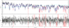 |
Fig. 1 LASP fitting result of an SB2 spectrum. The upper panel is the spectrum, and the lower panel is the fitting residual. The black line in the upper panel is the pseudo-continuum-normalised LAMOST MRS spectrum, the blue line is the best fitting spectrum, and the cyan line represents the polynomial correction between the observed spectrum and the model. Red lines in both panels represent the masked wavelength. |
2 Method
2.1 Data
The sources in this work are observed by both LAMOST MRS, Kepler mission and Kepler’s second mission (Kepler/K2; Batalha et al. 2010; Caldwell et al. 2010; Borucki et al. 2011), Transiting Exoplanet Survey Satellite (TESS; Ricker et al. 2015; Lund et al. 2017; Oelkers & Stassun 2018; Stassun et al. 2018), and targets were chosen that have at least three SB2 spectra in LAMOST MRS DR7 in order that we may evaluate the self-consistency of our method.
2.2 Double-lined binary spectral model
A binary spectrum contains light from both component stars. The observed spectrum of each binary is affected by the distance to us, the stellar luminosity, and the spectral line profiles. The line profiles are determined based on atmospheric parameters such as effective temperature, surface gravity, metallicity, and so on. The spectroscopic model of the binary star can therefore be explained as follows:
 (1)
(1)
![Mathematical equation: $ {F_i}\left( \lambda \right) = C \cdot {L_i} \cdot {P_i}\left( {{\lambda _i},{T_{{\rm{eff,i}}}},\log \,\,{g_i},\left[ {{{\rm{M}} \mathord{\left/ {\vphantom {{\rm{M}} {\rm{H}}}} \right. \kern-\nulldelimiterspace} {\rm{H}}}} \right]} \right), $](/articles/aa/full_html/2023/03/aa43487-22/aa43487-22-eq2.png) (2)
(2)
where Fbinary in Eq. (1) is the flux of the binary; F1 and F2 are the respective fluxes of the component stars; λ is the observed wavelength; λi stands for the shifted wavelength of each component in a specific orbital phase; and C stands for the relationship between the luminosity and the observed flux. In the shorter wavelength range, C is considered a constant and depends on the distance of the binary from Earth. Therefore, C has the same value for each component star. Li represents the luminosity of each star. Pi means the spectral line profiles. In this work, we use Teff, log g, and [M/H] to generate the theoretical continuum and line profiles simultaneously. For a binary system, Teff and log g are derived for each component while the same [M/H] is assigned. We omit the projected stellar rotation velocity υsin,i to generate the line profiles. The degeneration in surface gravity, rotational velocity, line mixing in binary spectra, and line spread function (LSF) of telescopes in line broadening can affect the accurate measurement of log g. See Sect. 3.2 for more details. In a binary spectrum, the line profiles of one component will be affected by the line mixing and the continuum of the other. The Doppler shifts of the continuum caused by the relative motion in different orbital phases affect the profiles differently.
For spectra without absolute flux calibration, the spectra are pseudo-continuum normalised before deriving stellar parameters, and only the line features are used. After normalisation, the effect of distance can be ignored. The binary star model can be explained as:
 (3)
(3)
where fbinary is the normalised binary spectrum. To obtain the luminosity contribution  (i = 1 or 2) from each star, we choose to model the binary spectra of the detached eclipsing binaries, because the orbital parameters and luminosity contributions of the eclipsing binaries can be derived by combining the light curves and the radial velocity curves. In different phases, the component star in a detached system is not distorted significantly by the gravitation of its companion. When the stars are approximated as spheres, the projected areas of the component stars can be simply regarded as circular surfaces in the modelling.
When the light curve solution is obtained, the binary spectral model with continuum is described as:
![Mathematical equation: $ \matrix{ {{F_{{\rm{binary}}}}\left( \lambda \right) = {A_1} \cdot {L_1} \cdot {P_1}\left( {{\lambda _1},{T_{{\rm{eff,1}}}},\log \,\,{g_1},\left[ {{{\rm{M}} \mathord{\left/ {\vphantom {{\rm{M}} {\rm{H}}}} \right. \kern-\nulldelimiterspace} {\rm{H}}}} \right]} \right)} \hfill \cr {\quad \quad \quad \,\,\,\,\,\,\,\,\, + {A_2} \cdot {L_2} \cdot {P_2}\left( {{\lambda _2},{r_{\rm{T}}} \cdot {T_{{\rm{eff,1}}}},\log \,\,{g_2},\left[ {{{\rm{M}} \mathord{\left/ {\vphantom {{\rm{M}} {\rm{H}}}} \right. \kern-\nulldelimiterspace} {\rm{H}}}} \right]} \right),} \hfill \cr } $](/articles/aa/full_html/2023/03/aa43487-22/aa43487-22-eq5.png) (4)
(4)
and then this model spectrum is pseudo-normalised to derive stellar parameters. In this model, the luminosity contribution of each component is determined not only based on its intrinsic brightness (Li) but also on the projection area (Ai) in a specific phase. A1 and A2 are calculated using stellar radii R1 and R2. The radii are obtained by analysing the orbital motion of the binary system. The light curves used in this work are from Kepler/K2 or the TESS mission, and the radial velocity curves are reconstructed using multi-epoch LAMOST MRS SB2 spectra. We use Wilson–Devinney binary star modelling code (WD; Wilson & Devinney 1971; Wilson 1979, 1990, 2008; Wilson & Van Hamme 2014) through a Python UI, PyWD2015 (Güzel & Özdarcan 2020), in order to derive the orbital parameters. After analysing the light curve, we get orbital period P, stellar radii R1 and R2, semi-major axis SMA, orbital inclination i, eccentricity e, periastron longitude ω, mass ratio q, and Teff ratio rT for the next steps. The observation epoch of the spectrum is folded into phase angle θ.
The theoretical model is computed using the SPECTRUM (Gray 2015) base on the Kurucz ATLAS9 (Castelli & Kurucz 2003), assuming local thermodynamic equilibrium (LTE) and a plane-parallel atmosphere to generate the flux density spectra. We then use the Payne (Ting et al. 2019) to interpolate the spectra of the component stars. The Payne is a stellar label fitting method that consists of several ingredients. The ‘interpolator’ of the Payne applies neural networks to produce spectral model fluxes for a set of arbitrary labels. The default neural network architectures, which have two hidden layers and ten neurons for each layer, are adopted in this work. The training set of the Payne is the Kurucz model mentioned above and the labels are Teff, log g, and [M/H], and the parameter ranges of the training set are: 4500 ≤ Teff ≤ 8000 K, 2.0 ≤ log g ≤ 5.0 dex, −2.0 ≤ [M/H] ≤ 0.5 dex. The ranges cover most of the LAMOST MRS observation data. Figure 2 shows the released stellar parameter distribution of LAMOST MRS DR7 v2.0. We ignore the spectral model with Teff lower than 4500 K because the mixing of the molecular bands will be more complicated. After the single star spectra are interpolated by the Payne, we synthesise the SB2 spectra with different RVs for the component stars and the projection areas that are calculated applying the light-curve solution. The pseudo-continuum-normalised SB2 spectra are used to fit the observed spectra with the least square method. The SB2 model generation and the spectral fitting are iterative. In each iteration, we synthesise the SB2 model with a new set of parameters to fit the observed spectra. Both blue and red bands are generated and applied in the fitting. This is unlike the LASP, which uses only the blue band in the fitting procedure. Although the LAMOST blue band contains more information than its red band in parameter deriving (Zhang et al. 2020), the blue band is not sufficiently sensitive to luminosity. Chen et al. (2021) suggested that the red band should also be used to derive atmospheric parameters, especially log g.
In Eq. (4), λ1 and λ2 are the shifted wavelengths of the component stars caused by their radial velocities RV1 and RV2. The radial velocities are automatically determined in the fitting procedure. Teff1 is the effective temperature of the hotter star and the effective temperature of the cooler star is represented by rT · Teff1. The initial value of rT comes from the light-curve solution, and we set it to be variable in the range ±0.1, although the true ratio of Teff is constant. The variation of rT actually reflects the change in the relative shift of two continua in the SB2 spectra. The application of rT can limit the spectral interpolation by the light curve characteristics and reduce the iteration times. log g1 and log g2 are the surface gravity of the two stars, respectively. Only one metallicity is derived for each spectrum.
In the non-eclipsing phases, the two component stars contribute all their fluxes to the binary spectrum. The projection area Ai is calculated according to the area of the circle. While in the eclipsing phases, eclipsing depth and surface blocking should be considered in luminosity contribution. When judging the relative distance d of the component stars, the eclipsing area can be calculated simultaneously, and d can be calculated using Eq. (A.4). Assuming that R1 > R2, the relative positions of the component stars are obtained by comparing the values of d, R1 + R2, and R1 − R2: (a) d > (R1 + R2): the luminosity distribution in non-eclipsing phases is discussed before. (b) d < (R1 − R2): the total eclipsing phase. (c) (R1 + R2) > d > (R1 − R2): during the partially eclipsing phases, the shielded areas are approximated to the area of a portion of a circle cut by a line segment. The area calculations are described in Appendix A.
We do not consider the reflection effect and the limb-darkening effect in this work, although they should be taken into consideration for the eclipsing phase spectra. Double-lined features in one spectrum indicate that the component stars have similar luminosity. Otherwise, the features of the least luminous star would be veiled by the other. Sometimes, the temperature difference between the primary and secondary star can be large for the situation where the cooler star has a larger radius than the hotter star. In the eclipsing phases, the reflection effect may change the magnitudes and thus the luminosity contributions. Also, in these phases, the limb-darkening effect may reduce the luminosity contribution of the eclipsed star, which increases the difficulty of deriving its atmospheric parameters. For the LAMOST MRS spectra, when ∆RV between the two stars is smaller than 50 km s−1, the stellar parameters derived by fitting the asymmetry of blended lines are quite different from those derived by fitting the double-lined features (see Appendix B). This may be caused by the resolving power or the noise of the spectra. The parameters from the blended lines are excluded in the final results, and the neglect of the reflection effect and the limb-darkening effect is ignored for LAMOST MRS SB2 spectra, but we note that for the data with higher resolution, these effects should be considered more carefully.
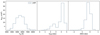 |
Fig. 2 Stellar parameter distribution derived by the LASP. The data used here are from LAMOST MRS Stellar Parameter Catalogue DR7 v2.0. |
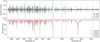 |
Fig. 3 The lines to obtain the line intensity ratios. The upper panel shows the gradient of line intensity differences of four Teff gaps: 7000–50/100/200/500 K. The lower panel contains the corresponding spectra. Different colours represent spectra with different Teff. The grey dashed lines indicate the spectral lines we chose to produce Figs. 4 and 5. |
2.3 Continuum influence and method uncertainty
In this subsection, we analyse the impact of the continuum in detail because the pseudo-normalised spectra are used in the fitting, and the line intensities of the normalised spectra will be significantly affected by the continuum. In an SB2 spectrum, the most luminous star makes the greatest contribution to the continuum and will cause more impact on line intensity after normalisation. The superposition of two continua causes the relative line intensity ratio between two stars in a binary spectrum to be lower than the ratio between the two single star spectra. We synthesised a series of SB2 spectra and fitted the double-peaked lines with the double-Gaussian function to see how the effect caused by luminosity and continuum varies with Teff and stellar radius. Figure 3 shows the lines we chose to obtain the line intensity ratios. The upper panel of Fig. 3 shows the gradient of line intensity differences of four Teff gaps: 7000–50/100/200/500 K. The differences were calculated after each theoretical spectrum was normalised using the pseudo-continuum. We derived the gradient to find the narrow single lines that are most sensitive to effective temperature changes. If a spectral line is sensitive to changes in Teff, the gradient shown in the upper panel of Fig. 3 will be higher. The lower panel contains the related theoretical spectra in the LAMOST MRS wavelength and resolving power. Four narrow single spectral lines that are sensitive to changes in Teff and are less contaminated by nearby lines were selected, and they are marked by the grey dashed lines. We then generated a series of SB2 spectra using the same model spectra as in our fitting procedures. The chosen stellar parameter ranges that are commonly contained in the LAMOST MRS DR7 data (Fig. 2) are as follows:
- (a)
The metallicity is fixed to −0.5 dex to reduce the fitting time.
- (b)
To analyse the effect from different effective temperatures, we initially set the primary star with Teff = 7250 K (Teff for an F0 dwarf star) and let the secondary star have a varying Teff from 5350 K (Teff for a G9 dwarf star) to 7250 K, with a step of 5 K. We then choose log g equal to 4.25 dex and 3.80 dex to represent the dwarf star and the subgiant star, respectively. According to the MESA Isochrones and Stellar Tracks (MIST; Dotter 2016; Choi et al. 2016), when the primary star is a 7250 K dwarf, it has a radius of 1.25 R⊙, and if the star is a 7250 K sub-giant, the radius is set to be 2.2 R⊙. As for the secondary star, we also set the radius to 1.2 R⊙ and 2.2 R⊙ for dwarf stars and subgiant stars, respectively. We fix the radius of the secondary star to reduce the affect of the stellar radius on the luminosity. The setup is not always physical but is reasonable in most cases. Next, we generate the double-lined features with ∆RV between the two component stars equal to 100 km s−1, which is twice the ∆RV detection limitation of the LAMOST MRS SB2 spectra in order to get better spectral line fitting. The SB2 spectra contain four combinations: dwarf + dwarf, subgiant + subgiant, dwarf + subgiant, and subgiant + dwarf for the primary and the secondary star, respectively. We have 1520 parameter combinations to investigate the affect of varying Teff.
- (c)
We also generated SB2 spectra with various radii to analyse the effect of the stellar radius. The parameter ranges are also from the MIST, although some specific combinations are not physical. To achieve a more prominent affect, we set the radius of the 7250 K primary star to vary from 1.2 R⊙ to 3.7 R⊙ with a step of 0.02 R⊙, and the related surface gravity is between 3.5 dex and 4.3 dex. The secondary star has a Teff of 6000 K (for a G0 dwarf star). The log g of a dwarf secondary star is 4.25 dex (R = 1.2 R⊙) and of a subgiant secondary is 3.80 dex (R = 2.2 R⊙), the same as in the case where we vary Teff. The combinations to generate binary spectra are 7250 K primary star + dwarf secondary star and 7250 K primary star + giant secondary star. We have 254 parameter combinations for the radius-changing affect.
- (d)
In different orbital phases, the relative motions between the two component stars cause the continuum of the most luminous star to blue- or redshift in the binary spectra. To analyse whether or not the blue- or redshifted continua have varying effect on the line intensities, the synthesised SB2 spectra have two kinds of radial velocity settings: the primary star has a radial velocity of −50 km s−1 and +50 km s−1. ∆RV between the two components is 100 km s−1. This procedure doubles the SB2 spectral number, and so we finally have 3548 SB2 spectra for the line intensity ratio analysis, including 3040 spectra with various Teff and 508 with various radii. Figure 4 shows how the line ratios change with different Teff, and Fig. 5 shows the changes with varying radii.
- (e)
With the same atmospheric parameters and stellar radius, but with ∆RV varying from 40 km s−1 to 120 km s−1 randomly, we generated another 3548 SB2 spectra to evaluate the parameter fitting accuracy of our method. Figures 6 and 7 show the differences between the theoretical parameters and the fitting parameters.
In Fig. 4, the line ratios of the different spectral lines with varying Teff are shown in separate panels. In each panel, different line styles represent different parameter combinations. Grey lines are the line intensity ratios between two spectra of single stars. The blue lines indicate that the 7250 K components are blueshifted in the SB2 spectra, and the orange lines mean the components are at the redshifted phases. In the normalised single star spectra, the relative line intensities of stars with lower Teff are stronger than those of the stars that have Teff = 7250 K. However, in an SB2 spectrum, the superposition of two continua will reduce the relative line intensities after normalisation. The blue and the orange lines mean that the line intensities of the least luminous star are reduced more than the line intensities of the most luminous.
Figure 5 shows how the line intensity ratios change with different radii. Line styles and colours in this figure have the same meaning as in Fig. 4. The line intensity ratios do not vary significantly with stellar radius, which may be the result of our narrow radius selection range. The differences between the grey and the blue/orange lines also mean that the superposed continuum has more affect on the line intensities of the least luminous star.
Although the line intensities of the least luminous star are significantly reduced in the binary spectra, the blue and orange lines that have the same line styles in Figs. 4 and 5 show that the line intensity decrease does not vary significantly in different orbital phases. The atmospheric parameters derived in different phases (and with various ∆RV) should be consistent as long as the components can be detected. Figure 6 shows the atmospheric parameter differences of the synthetic SB2 spectra when the primary stars are in blueshifted phases, and Fig. 7 shows the parameter differences when the primary stars are at redshifted phases. Each panel contains the parameter from the fitting results of both the primary and the secondary star. The figures show that if the stellar radius and luminosity contribution are known, the fitting results will have very low-level uncertainties for spectra without noise. We therefore do not consider the method uncertainties in the application on the observed SB2 spectra.
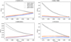 |
Fig. 4 Line intensity ratio between a lower Teff star and a 7250 K star. The grey lines represent the ratio between two spectra of single stars, and the colourful lines are the ratio between two star components in the binary spectra. The blue lines mean that the 7250 K components are blueshifted in SB2 spectra, and the orange lines mean that the 7250 K components are redshifted. Different line styles stand for different parameter combinations. |
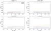 |
Fig. 5 Line intensity ratios change with different radii. The grey lines represent the ratio between two spectra of single stars, and the colourful lines are the ratio between two star components in the binary spectra. The blue lines mean that the 7250 K components are blueshifted in SB2 spectra, and the orange lines mean that the 7250 K components are redshifted. Different line styles stand for different parameter combinations. |
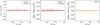 |
Fig. 6 Parameter differences between the measured values and the theoretical values. Blue circles in ∆Teff and ∆ log g panels show the differences between the primary stars, and orange dots show the differences between the secondary stars. One metallicity is fitted for each binary system, so the ∆[M/H] panels contain only orange points. All the binaries in this figure have the primary component blueshifted in the SB2 spectra. |
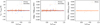 |
Fig. 7 Parameter differences between the measured values and the theoretical values. Colours and symbols have the same meaning as in Fig. 6. All the binaries in this figure have the primary component redshifted in the SB2 spectra. |
3 Examples: Atmospheric parameters of two SB2 eclipsing systems
In this section, we give two observation examples of eclipsing binaries in order to demonstrate the ability of our method. The examples are chosen randomly because the method is designed for binary stars that match our criteria in Sect. 2. Both of the binaries have at least three SB2 spectra in LAMOST MRS DR7 and have light curves from Kepler/K2 or TESS.
3.1 TIC 63209649
TIC 63209649 (also known as KIC 8301013, but TESS light curves are used in this work, so we give the TIC number) is a detached eclipsing binary system with nine successful epochs of spectra in the LAMOST MRS DR7. Figures 8–10 show the observation data. Figure 8 is the normalised TESS light curve. This system has a period of about 4.43 days. Figure 9 shows the normalised LAMOST MRS spectra of nine epochs. The spectra are listed in the observed time sequence, and the observation time in UTC format is shown in the upper right corner. Figure 10 shows the radial velocities of component stars in phase view. In order to reconstruct the RV curve, we firstly use the Payne and our binary spectral model to fit each binary spectrum. The centres of strong lines can be fitted correctly to obtain the radial velocities of each star. We then use  to fit q and γ. Here, RV1 and RV2 are the radial velocities of the primary star and the secondary star folded in the phase order, respectively. In addition to the three dots in phases 0, 0.5, and 1, other dots in Fig. 10 are the measured RVs. The three dots are set manually to be γ. Finally, we reconstruct the RV curve using cosine functions. The standard deviation between the measured RVs and the best fitting lines is 5.08 km s−1 for RV1 and 6.66 km s−1 for RV2. We note that the fitting may be rough at the near-eclipsing phases. Combining the light curve and the radial-velocity curves, we derived all the orbital parameters using the WD modelling. Figure 11 is the WD fitting result. Black dots in the upper panel represent the folded light curve, and the red line is the best fitting model. Dots in the lower panel are the residuals. The orbital parameters from the light-curve solution are listed in Table 1. Combining the orbital parameters, we generated the synthetic SB2 model spectra according to Eq. (4), and fitted seven multi-epoch SB2 spectra of TIC 63209649. Figure 12 shows the best fitting result of one of the SB2 epochs. Black lines are the observed spectra of blue (upper panel) and red (lower panel) bands, and the red lines represent the best fitting spectra. Grey dots indicate the percentage of the residual in the observed data. Most of the residuals are below 10% of the observed spectra, except for residuals of some strong lines, such as the Mg I triplet, λ5167, 72, and 83 and the Hα line. In wavebands with dense spectral lines, for example, λ5175 ~ 5180 and λ5280 ~ 5285, line mixing causes the fitting residuals to become a slightly higher than the relatively lineless waveband. Two of the nine epochs were observed near eclipsing phases and did not show clear double-lined features. We present the spectral fitting results in Appendix B and give a brief discussion.
Derived atmospheric parameters of all the SB2 spectra of TIC 63209649 are listed in Table 2 in order of observation time. The orbital phases are shown in the second column. Teff1 and log g1 are the parameters of the hotter star, and the parameters of the cooler one are Teff2 and log g2. The metallicity of the binary system is [M/H]. The parameters of the first four epochs show good consistency, but the results of the last three epochs are different, and they are labelled with asterisks in the first column. We checked the spectra of these three epochs and found that a poor signal-to-noise ratio might be the reason for this inconsistency. Figure 13 shows the fitting result of the last spectrum (MJD = 58 645) in Table 2. The noise in this spectrum is higher compared with that in Fig. 12. We therefore excluded this spectrum as well as the two previous noisy spectra before parameter averaging. Atmospheric parameters in the last row of Table 2 are the mean values of the adopted epoch results. We take the standard deviations as the measurement errors and list them in the parentheses. The errors are at the same level as the errors of the LASP parameters of the single stars (Chen et al. 2021).
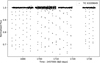 |
Fig. 8 Normalised TESS light curve of TIC 63209649. |
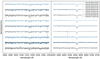 |
Fig. 9 Pseudo-continuum normalised LAMOST MRS multi-epoch spectra of TIC 63209649. The spectra are shown in the same order in which they were observed. |
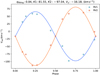 |
Fig. 10 Reconstructed radial velocity curves of TIC 63209649. Dots are the RVs measured by the spectra except for three dots in the phases 0, 0.5, and 1, which are set manually to γ. Lines are the reconstructed curves. Blue represents the higher mass star and orange represents the lower mass star. |
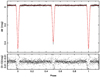 |
Fig. 11 WD fitting result of the TIC 63209649 light curve. Black dots in the upper panel are the observed data and the red line is the best fitting model. The lower panel shows the fitting residuals. |
Orbital parameters of TIC 63209649.
3.2 EPIC 247529791
The K2 target EPIC 247529791 is also a detached eclipsing binary with a nearly circular orbit. Figure 14 is the normalised K2 light curve. The orbital period is 3.94 days. Figure 15 shows LAMOST MRS spectra of five epochs in time sequence. The latest spectrum has a poor signal-to-noise ratio, and so we excluded it from the fitting procedures. Figure 16 shows the reconstructed radial velocity curves. The curves are fitted using the same procedure as in Sect. 3.1 and the symbols and lines have the same meaning as in Fig. 10. The standard deviation between the measured RVs and the best fitting lines are 0.33 km s−1 for RV1 and 0.98 km s−1 for RV2. The orbital parameters are also derived using WD and Fig. 17 is the best fitting model. The orbital parameters are listed in Table 3. The model synthesis and spectral fitting is the same as above. Three of the four higher signal-to-noise ratio (S/N) spectra show double-lined features and are used to derive stellar parameters. Figure 18 is an example of a best fitting result. In most of the wavelengths, the residuals have the same level as in Fig. 12. The fitting result of the unresolved spectrum is also discussed in Appendix B.
Table 4 shows the atmospheric parameters of SB2 spectral fitting. Teff and [M/H] derived from different phases show good consistency, but log g of the secondary star cannot be derived robustly. Two factors may explain this phenomenon. First, the lower S/N influences the fitting result substantially. Second, the most prominent line features in the LAMOST MRS spectra are the Mg I triplet, λ5167, 72, 83 lines in the blue band, and the Hα line in the red band. The Mg I triplet lines are not sensitive enough to luminosity (Guinan & Smith 1984), and their line profiles are easily influenced when ∆RV between component stars gets larger. Although combining the red band in the fitting procedure can improve the log g derivation (Chen et al. (2021), Figs. 11–12), the wings of the Ha line are also significantly affected by the mixing of two components.
The atmospheric parameters of component stars in the EPIC 247529791 system were also derived by (Traven et al. 2020, hereafter Traven 2020). The GALAH DR2 specID of this binary is 17013100180129. The authors of this latter work used photometry data to reconstruct the SED of the binaries and then applied the Bayesian inference and a Monte Carlo Markov chain sampler (Gregory 2005; Hogg et al. 2010; Foreman-Mackey et al. 2013; Sharma 2017) to derive atmospheric parameters. The Traven 2020 parameters are listed in Table 5. Metallicities of the system derived in our work and by Traven 2020 show good consistency. For the warmer component star, our method gets higher Teff than that of Traven 2020, while for the cooler star, our Teff is lower than that of Traven 2020. The log g of the warmer star obtained by the two methods is similar. The log g of the cooler star in our results is lower than that found by Traven 2020. Furthermore, both log g of the cooler star derived in the two works is lower than that in the light curve solution in Table 3.
Different resolving power and fitting methods may cause the inconsistency of the derived parameters. (1) The LAMOST MRS with R ~ 7500 has a lower resolution than GALAH (R ~ 28 000). Line mixing caused by the Doppler shift of the component stars makes recognising features of the fainter star more difficult, and makes deriving atmospheric parameters imprecise in the lower resolution spectra. (2) We use the Kurucz theoretical spectra as our fitting model, while Traven 2020 adopted a series of observed spectra as the fitting template, which is the same as in the GALAH official pipeline (Kos et al. 2017). (3) The binary spectra models are produced in different ways. In our work, we synthesise the binary spectra with the light-curve-derived radii and the phase-based projection areas. The luminosity contribution depends on the real size and Teff ratio of the component stars. Traven 2020 generated the synthetic SED of two single stars using the Kurucz ATLAS9 models and produced the SED of the binary system taking the component star radii as the independent variables. The generated binary SED and the radii were restricted by the apparent magnitudes from AAVSO Photometric All-Sky Survey (APASS; Henden et al. 2016), Gaia DR2 (Evans et al. 2018), Two Micron All Sky Survey (2MASS; Skrutskie et al. 2006), and Wide-field Infrared Survey Explorer (WISE; Wright et al. 2010).
Except for the difference between the two methods, we suggest two other factors that may cause the inconsistency. These two factors may also represent disadvantages to deriving atmospheric parameters using SB2 spectra. Firstly, the effect of mixing and continuum contamination on the line depth influence the measurement of Teff. Theoretically, the prime criteria used to derive the effective temperature for a main sequence F-type star are the strength and profiles of the hydrogen lines (Gray & Corbally 2009). But the LAMOST MRS waveband contains only the Hα line. Due to its depth and broad width, the Hα line is easily influenced by the mixing of two spectra. In this case, the metal lines become the main features used to derive Teff. But metal lines are shallower than the Hα lines; the absolute strength is more easily affected by the continuum. Furthermore, the relative line intensity ratio is constrained by the luminosity contribution. When fitting the SB2 spectrum, the most luminous star component occupies more weight in fitting the best model. This makes the measured Teff of the hotter star higher than the real value. These two factors, that is the relative line intensity change and the higher measured Teff of the hotter star, cause the Teff ratio to get smaller in the fitting iteration, which causes the Teff measurement of the cooler star to be lower. Absolute flux calibration may help to reduce continuum contamination.
Secondly, the surface gravity of the component stars found by fitting the SB2 spectra are underestimated. As the most prominent spectral lines in the LAMOST MRS waveband are the MgI triplet λλ 5167, 72, 83 and the Hα, the surface gravity of most of the A- to G-type main-sequence stars cannot be derived precisely (Chen et al. 2021). The wings of the hydrogen lines are sensitive to luminosity for early A-type stars, as is the MgI triplet for late G- to mid-K-type stars (Guinan & Smith 1984). Furthermore, the micro-turbulent velocity plays an important role in determining surface gravity for the F-, G-, and even K-type stars. For the mid-F-type dwarfs, a micro-turbulent velocity of about 2 km s−1 affects the luminosity criteria (Gray et al. 2001). The spectral lines in a single star spectrum are broader and stronger due to the micro-turbulence. In an SB2 spectrum, Doppler shift and line mixing cause the double-peaked lines to be broader and stronger than the lines in a single-star spectrum. Under the joint influence of the micro-turbulence and the line mixing, deriving log g directly from the SB2 spectra underestimates the measured results. Although Traven 2020 accounted for the micro-turbulent velocity, the spectral line mixing still makes sense, resulting in log g measurements that are smaller than the light curve solution.
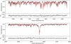 |
Fig. 12 Best fitting example of the TIC 63209649 SB2 spectrum. Black lines are the LAMOST MRS spectra and red lines are the best fitting synthetic SB2 model. Grey dots represent the fitting residuals. |
Atmospheric parameters of the TIC 63209649 component stars.
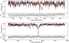 |
Fig. 13 Fitting example of a TIC 63209649 spectrum with a low signal-to-noise ratio. Colours and symbols have the same meaning as in Fig. 12. |
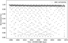 |
Fig. 14 Normalised K2 light curve of EPIC 247529791. |
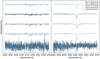 |
Fig. 15 Pseudo-continuum-normalised LAMOST MRS multi-epoch spectra of EPIC 247529791. The spectra are shown in the same order as the observations. |
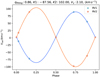 |
Fig. 16 Reconstructed radial velocity curves of EPIC 247529791. Dots are the RVs measured from the spectra except for three dots in the phases 0, 0.5, and 1, which are set manually to γ. Lines are the reconstructed curves. Blue represents the higher mass star and orange represents the lower mass star, respectively. |
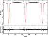 |
Fig. 17 WD fitting result of the EPIC 247529791 light curve. Black dots in the upper panel are the observed data and the red line is the best fitting model. The lower panel shows the fitting residuals. |
Orbital parameters of EPIC 247529791.
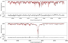 |
Fig. 18 Best fitting example of the EPIC 247529791 SB2 spectrum. Black lines are the LAMOST MRS spectra and red lines are the best fitting synthetic SB2 model. Grey dots represent the fitting residuals. |
Atmospheric parameters of the EPIC 247529791 component stars.
Atmospheric parameters of the EPIC 247529791 derived by Traven2020.
4 Summary
We provide a method to model the binary star spectra with double-lined features. The antecedent information of a detached eclipsing binary system is derived by solving the light curves and radial velocity curves. We synthesise the SB2 model spectra by superposing single star spectra according to the luminosity contribution of the component stars. The synthetic spectra are then used to fit the observation spectra using the least square method and to derive atmospheric parameters of the component stars. The method provides the radial velocities, effective temperatures, and surface gravity of each star, and metallicity for the binary system. We generate model spectra for different phases according to the change of the relative position of the component stars. The atmospheric parameters derived from the multi-epoch SB2 spectra have similar values, which indicates the robustness of our method.
Our method provides a way to calculate effective projection areas of component stars in both eclipsing and non-eclipsing phases. However, in the fitting experiments shown in Sect. 3, we find that the LAMOST MRS SB2 spectra were observed mostly in the non-eclipsing phases. With a resolution of 7500, LAMOST MRS cannot resolve double-lined features in nearly eclipsing phases. Therefore, the LAMOST MRS SB2 spectra contain fluxes from the whole system of stars.
This method can also be applied to partially eclipsing spectra as long as the resolution is high enough to resolve binary features. In addition, with increasing resolution, the influence of the limb-darkening effect, the reflection between two stars, and the microturbulence on the spectral line begin to appear and should be considered in determining atmospheric parameters.
Acknowledgements
The authors thank the reviewer for useful comments to the manuscript. This work is supported by National Science Foundation of China (Nos. U1931209, 11970360, 12003050, 12090044, 12103068) and National Key R&D Program of China (Nos. 2019YFA0405102, 2019YFA0405502). Guoshoujing Telescope (the Large Sky Area Multi-Object Fibre Spectroscopic Telescope, LAMOST) is a National Major Scientific Project built by the Chinese Academy of Sciences. Funding for the project has been provided by the National Development and Reform Commission. LAMOST is operated and managed by the National Astronomical Observatories, Chinese Academy of Sciences. This paper includes data collected by the Kepler mission and obtained from the MAST data archive at the Space Telescope Science Institute (STScI). Funding for the Kepler mission is provided by the NASA Science Mission Directorate. STScI is operated by the Association of Universities for Research in Astronomy, Inc., under NASA contract NAS 5-26555. This paper includes data collected with the TESS mission, obtained from the MAST data archive at the Space Telescope Science Institute (STScI). Funding for the TESS mission is provided by the NASA Explorer Program. STScI is operated by the Association of Universities for Research in Astronomy, Inc., under NASA contract NAS 5-26555.
Appendix A Projection area calculation
1. Basic assumptions: spherical component stars.
2. Initial data.
2.1 Fit RV curves and mass ratio q using spectra radial velocities.
2.2 Period (P), eccentricity (e), inclination (i), argument of periastron (ω), time of periastron passage tper, semi major axis (SMA), radii of component stars (suppose R1 > R2).
3. Projection areas.
Figure A.1 is a schematic of the projection areas during shallow partial eclipse. The specific calculation is as follows:
3.1 At the observation time t of an SB2 spectrum, the mean anomaly M, the eccentric anomaly E, and the true anomaly υ of the binary system are calculated as follows:
 (A.1)
(A.1)
 (A.2)
(A.2)
 (A.3)
(A.3)
3.2 Projection distance d between the component stars onto the plane-of-sky:
![Mathematical equation: $ d = SMA{{1 - {e^2}} \over {1 + e\cos \upsilon }}{\left[ {1 - {{\sin }^2}\left( {\omega + \upsilon } \right){{\sin }^2}i} \right]^a} $](/articles/aa/full_html/2023/03/aa43487-22/aa43487-22-eq10.png) (A.4)
(A.4)
3.3 Projection areas during different phases:
3.3.1 No eclipse (d > R1 + R2):
 (A.5)
(A.5)
3.3.2 Total and annular eclipse (d < R1 − R2):
 (A.6)
(A.6)
When the larger star is in front (total eclipse):
When the smaller star is in front (annular eclipse):
 (A.7)
(A.7)
3.3.3 Partial eclipse:
a.Shallow partial eclipse  :
:
Larger star in front:
 (A.8)
(A.8)
Smaller star in front:
 (A.9)
(A.9)
b.Deep partial eclipse  :
:
Larger star in front:
 (A.10)
Smaller star in front:
 (A.11)
∆A1 and ∆A2 are approximated to the area of a portion of a circle cut by a line segment.
 (A.12)
n1 and n2 (in radian) in the above equations represent the central angle corresponding to the chord where the two circles intersect on each projection of the stellar surface. They can be calculated as follows:
 (A.13)
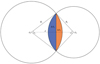 |
Fig. A.1 Schematic diagram of the projection areas. O1 and O2 represent the projected centres of the stellar discs, and d is the distance between them. R1 and R2 stand for the radii of the component stars. The areas ∆A1 and ∆A2 vary in different orbital phases. See step 3 in Appendix A for their calculation. |
Appendix B Fitting spectra from near-eclipsing phases
At the near-eclipsing phases, although the double-line features cannot be recognised in the LAMOST MRS resolution, the asymmetry of lines is caused when ∆RV < 50 km s−1. We present the spectral fitting results of two near-eclipsing spectra. Figure B.1 shows the best fitting model of a TIC 63209649 spectrum. The black lines are the LAMOST MRS spectra, the red dashed lines are the best fitting model, and the grey dotted lines represent the residuals. Although the spectrum can be fitted by a synthetic binary spectrum with the help of the orbital results, the atmospheric parameters are quite different from the results of the SB2 spectra. The best fitting parameters of Figure B.1 are: Teff1 = 6263.63 K, log g1 = 3.75 dex for the primary star, Teff2 = 6220.43 K, log g2 = 4.44 dex for the secondary star, and [M/H] = −0.48 dex for the binary system. But the mean parameters of the SB2 spectral fitting are: Teff1 = 6643.22 ± 49.20 K, log g1 = 4.13 ± 0.13 dex for the primary star, Teff2 = 5917.39 ± 37.60 K, log g2 = 3.78 ± 0.04 dex for the secondary star, and [M/H] = −0.23 ± 0.13 dex for the binary system (Table 2). In Sect. 2.3, we find the atmospheric parameters derived in different phases should not vary significantly if the contributions of the component stars are detected correctly. Therefore, the fitting results in the figure are likely to be inconsistent with the real situation. We suggest that the real signal-to-noise ratio (S/N) of the near-eclipsing spectrum is not high enough to recognise the line asymmetry correctly, despite the announced S/N of this spectrum being 60.42 for the blue band and 94.05 for the red band in the LAMOST MRS catalogue.
Figure B.2 is the near-eclipsing phase fitting result of EPIC 247529791. The atmospheric parameters fitted from these spectra are also different from the parameters from the SB2 spectra. The best fitting parameters of Figure B.2 are: Teff1 = 6905.15 K, log g1 = 3.60 dex for the primary star, Teff2 = 6367.69 K, log g2 = 3.32 dex for the secondary star, and [M/H] = −0.31 dex for the binary system. But the mean parameters of the SB2 spectral fitting are: Teff1 = 6969.73 ± 16.30 K, log g1 = 3.56 ± 0.06 dex for the primary star, Teff2 = 6146.84 ± 38.50 K, log g2 = 3.39 ± 0.30 dex for the secondary star, and [M/H] = −0.46 ± 0.02 dex for the binary system (Table 4). We do not use the parameters of the near-eclipsing spectra to calculate the final parameters in this work, but we note that our method has the ability to deal with the line-asymmetry spectra with more precise orbital parameters and high-S/N spectra.
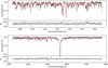 |
Fig. B.1 Best fitting result of TIC 63209649 at the near-eclipsing phase. Lines and colours have the same meaning as in Figure 12. This spectrum is also the fifth from the top in Figure 9. The orbital phase of this spectrum is 0.9931. |
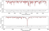 |
Fig. B.2 Best fitting result of EPIC 247529791 at the near-eclipsing phase. Lines and colours have the same meaning as in Figure B.1. This spectrum is also the fourth from the top in Figure 15 The orbital phase of this spectrum is 0.0260. |
References
- Batalha, N. M., Borucki, W. J., Koch, D. G., et al. 2010, ApJ, 713, L109 [NASA ADS] [CrossRef] [Google Scholar]
- Borucki, W. J., Koch, D. G., Basri, G., et al. 2011, ApJ, 736, 19 [Google Scholar]
- Caldwell, D. A., Kolodziejczak, J. J., Van Cleve, J. E., et al. 2010, ApJ, 713, L92 [NASA ADS] [CrossRef] [Google Scholar]
- Castelli, F., & Kurucz, R. L. 2003, in Modelling of Stellar Atmospheres, eds. N. Piskunov, W. W. Weiss, & D. F. Gray (ASP), 210, A20 [Google Scholar]
- Chen, H.-L., Woods, T. E., Yungelson, L. R., Gilfanov, M., & Han, Z. 2015, MNRAS, 453, 3024 [Google Scholar]
- Chen, X.-L., Luo, A. L., Chen, J.-J., et al. 2021, PASP, 133, 044502 [NASA ADS] [CrossRef] [Google Scholar]
- Choi, J., Dotter, A., Conroy, C., et al. 2016, ApJ, 823, 102 [Google Scholar]
- Dotter, A. 2016, ApJS, 222, 8 [Google Scholar]
- Duchêne, G., & Kraus, A. 2013, ARA&A, 51, 269 [Google Scholar]
- El-Badry, K., Ting, Y.-S., Rix, H.-W., et al. 2018, MNRAS, 476, 528 [Google Scholar]
- Evans, D. W., Riello, M., De Angeli, F., et al. 2018, A&A, 616, A4 [NASA ADS] [CrossRef] [EDP Sciences] [Google Scholar]
- Foreman-Mackey, D., Hogg, D. W., Lang, D., & Goodman, J. 2013, PASP, 125, 306 [Google Scholar]
- Götberg, Y., de Mink, S. E., McQuinn, M., et al. 2020, A&A, 634, A134 [EDP Sciences] [Google Scholar]
- Gray, R. 2015, Documentation for Spectrum v2.76, DOI: https://doi.org/10.13140/RG.2.1.1198.0242 [Google Scholar]
- Gray, R., & Corbally, C. 2009, Stellar Spectral Classification (Princeton University Press) [CrossRef] [Google Scholar]
- Gray, R. O., Graham, P. W., & Hoyt, S. R. 2001, AJ, 121, 2159 [NASA ADS] [CrossRef] [Google Scholar]
- Gregory, P. 2005, The how-to of Bayesian Inference (Cambridge University Press), 41 [Google Scholar]
- Guinan, E. F., & Smith, G. H. 1984, PASP, 96, 354 [NASA ADS] [CrossRef] [Google Scholar]
- Güzel, O., & Özdarcan, O. 2020, Contrib. Astron. Observ. Skalnate Pleso, 50, 535 [Google Scholar]
- Han, Z. 1998, MNRAS, 296, 1019 [NASA ADS] [CrossRef] [Google Scholar]
- Han, Z., Podsiadlowski, P., & Lynas-Gray, A. E. 2007, MNRAS, 380, 1098 [NASA ADS] [CrossRef] [Google Scholar]
- Han, Z.-W., Ge, H.-W., Chen, X.-F., & Chen, H.-L. 2020, Res. Astron. Astrophys., 20, 161 [CrossRef] [Google Scholar]
- Henden, A. A., Templeton, M., Terrell, D., et al. 2016, VizieR Online Data Catalog: II/336 [Google Scholar]
- Hogg, D. W., Bovy, J., & Lang, D. 2010, ArXiv e-prints [arXiv: 1008.4686] [Google Scholar]
- Hoyle, F., & Fowler, W. A. 1960, ApJ, 132, 565 [NASA ADS] [CrossRef] [Google Scholar]
- Iben, I. J., & Tutukov, A. V. 1984, ApJS, 54, 335 [NASA ADS] [CrossRef] [Google Scholar]
- Izzard, R. G., Glebbeek, E., Stancliffe, R. J., & Pols, O. R. 2009, A&A, 508, 1359 [NASA ADS] [CrossRef] [EDP Sciences] [Google Scholar]
- Koch, D. G., Borucki, W. J., Basri, G., et al. 2010, ApJ, 713, L79 [Google Scholar]
- Kos, J., Lin, J., Zwitter, T., et al. 2017, MNRAS, 464, 1259 [NASA ADS] [CrossRef] [Google Scholar]
- Li, C.-Q., Shi, J.-R., Yan, H.-L., et al. 2021, ApJS, 256, 31 [NASA ADS] [CrossRef] [Google Scholar]
- Liu, C., Fu, J., Shi, J., et al. 2020, Res. Astron. Astrophys., submitted, [arXiv:2005.07210] [Google Scholar]
- Lund, M. N., Handberg, R., Kjeldsen, H., Chaplin, W. J., & Christensen-Dalsgaard, J. 2017, EPJ Web of Conferences, 160, 01005 [NASA ADS] [CrossRef] [EDP Sciences] [Google Scholar]
- Luo, A. L., Zhao, Y.-H., Zhao, G., et al. 2015, Res. Astron. Astrophys., 15, 1095 [Google Scholar]
- Oelkers, R. J., & Stassun, K. G. 2018, AJ, 156, 132 [NASA ADS] [CrossRef] [Google Scholar]
- Raghavan, D., McAlister, H. A., Henry, T. J., et al. 2010, ApJS, 190, 1 [Google Scholar]
- Ricker, G. R., Winn, J. N., Vanderspek, R., et al. 2015, J. Astron. Telesc. Instrum. Syst., 1, 014003 [Google Scholar]
- Secunda, A., Cen, R., Kimm, T., Götberg, Y., & de Mink, S. E. 2020, ApJ, 901, 72 [NASA ADS] [CrossRef] [Google Scholar]
- Sharma, S. 2017, ARA&A, 55, 213 [Google Scholar]
- Skrutskie, M. F., Cutri, R. M., Stiening, R., et al. 2006, AJ, 131, 1163 [NASA ADS] [CrossRef] [Google Scholar]
- Stassun, K. G., Oelkers, R. J., Pepper, J., et al. 2018, AJ, 156, 102 [Google Scholar]
- Ting, Y.-S., Conroy, C., Rix, H.-W., & Cargile, P. 2019, ApJ, 879, 69 [Google Scholar]
- Traven, G., Feltzing, S., Merle, T., et al. 2020, A&A, 638, A145 [NASA ADS] [CrossRef] [EDP Sciences] [Google Scholar]
- Webbink, R. F. 1984, ApJ, 277, 355 [NASA ADS] [CrossRef] [Google Scholar]
- Whelan, J., & Iben, Icko, Jr. 1973, ApJ, 186, 1007 [CrossRef] [Google Scholar]
- Wilson, R. E. 1979, ApJ, 234, 1054 [Google Scholar]
- Wilson, R. E. 1990, ApJ, 356, 613 [Google Scholar]
- Wilson, R. E. 2008, ApJ, 672, 575 [NASA ADS] [CrossRef] [Google Scholar]
- Wilson, R. E., & Devinney, E. J. 1971, ApJ, 166, 605 [Google Scholar]
- Wilson, R. E., & Van Hamme, W. 2014, ApJ, 780, 151 [Google Scholar]
- Wright, E. L., Eisenhardt, P. R. M., Mainzer, A. K., et al. 2010, AJ, 140, 1868 [Google Scholar]
- Wu, Y., Luo, A. L., Li, H.-N., et al. 2011, Res. Astron. Astrophys., 11, 924 [Google Scholar]
- Zhang, B., Liu, C., Li, C.-Q., et al. 2020, Res. Astron. Astrophys., 20, 051 [CrossRef] [Google Scholar]
- Zhang, B., Jing, Y.-J., Yang, F., et al. 2022, ApJS, 258, 26 [NASA ADS] [CrossRef] [Google Scholar]
All Tables
All Figures
|
Fig. 1 LASP fitting result of an SB2 spectrum. The upper panel is the spectrum, and the lower panel is the fitting residual. The black line in the upper panel is the pseudo-continuum-normalised LAMOST MRS spectrum, the blue line is the best fitting spectrum, and the cyan line represents the polynomial correction between the observed spectrum and the model. Red lines in both panels represent the masked wavelength. |
| In the text | |
|
Fig. 2 Stellar parameter distribution derived by the LASP. The data used here are from LAMOST MRS Stellar Parameter Catalogue DR7 v2.0. |
| In the text | |
|
Fig. 3 The lines to obtain the line intensity ratios. The upper panel shows the gradient of line intensity differences of four Teff gaps: 7000–50/100/200/500 K. The lower panel contains the corresponding spectra. Different colours represent spectra with different Teff. The grey dashed lines indicate the spectral lines we chose to produce Figs. 4 and 5. |
| In the text | |
|
Fig. 4 Line intensity ratio between a lower Teff star and a 7250 K star. The grey lines represent the ratio between two spectra of single stars, and the colourful lines are the ratio between two star components in the binary spectra. The blue lines mean that the 7250 K components are blueshifted in SB2 spectra, and the orange lines mean that the 7250 K components are redshifted. Different line styles stand for different parameter combinations. |
| In the text | |
|
Fig. 5 Line intensity ratios change with different radii. The grey lines represent the ratio between two spectra of single stars, and the colourful lines are the ratio between two star components in the binary spectra. The blue lines mean that the 7250 K components are blueshifted in SB2 spectra, and the orange lines mean that the 7250 K components are redshifted. Different line styles stand for different parameter combinations. |
| In the text | |
|
Fig. 6 Parameter differences between the measured values and the theoretical values. Blue circles in ∆Teff and ∆ log g panels show the differences between the primary stars, and orange dots show the differences between the secondary stars. One metallicity is fitted for each binary system, so the ∆[M/H] panels contain only orange points. All the binaries in this figure have the primary component blueshifted in the SB2 spectra. |
| In the text | |
|
Fig. 7 Parameter differences between the measured values and the theoretical values. Colours and symbols have the same meaning as in Fig. 6. All the binaries in this figure have the primary component redshifted in the SB2 spectra. |
| In the text | |
|
Fig. 8 Normalised TESS light curve of TIC 63209649. |
| In the text | |
|
Fig. 9 Pseudo-continuum normalised LAMOST MRS multi-epoch spectra of TIC 63209649. The spectra are shown in the same order in which they were observed. |
| In the text | |
|
Fig. 10 Reconstructed radial velocity curves of TIC 63209649. Dots are the RVs measured by the spectra except for three dots in the phases 0, 0.5, and 1, which are set manually to γ. Lines are the reconstructed curves. Blue represents the higher mass star and orange represents the lower mass star. |
| In the text | |
|
Fig. 11 WD fitting result of the TIC 63209649 light curve. Black dots in the upper panel are the observed data and the red line is the best fitting model. The lower panel shows the fitting residuals. |
| In the text | |
|
Fig. 12 Best fitting example of the TIC 63209649 SB2 spectrum. Black lines are the LAMOST MRS spectra and red lines are the best fitting synthetic SB2 model. Grey dots represent the fitting residuals. |
| In the text | |
|
Fig. 13 Fitting example of a TIC 63209649 spectrum with a low signal-to-noise ratio. Colours and symbols have the same meaning as in Fig. 12. |
| In the text | |
|
Fig. 14 Normalised K2 light curve of EPIC 247529791. |
| In the text | |
|
Fig. 15 Pseudo-continuum-normalised LAMOST MRS multi-epoch spectra of EPIC 247529791. The spectra are shown in the same order as the observations. |
| In the text | |
|
Fig. 16 Reconstructed radial velocity curves of EPIC 247529791. Dots are the RVs measured from the spectra except for three dots in the phases 0, 0.5, and 1, which are set manually to γ. Lines are the reconstructed curves. Blue represents the higher mass star and orange represents the lower mass star, respectively. |
| In the text | |
|
Fig. 17 WD fitting result of the EPIC 247529791 light curve. Black dots in the upper panel are the observed data and the red line is the best fitting model. The lower panel shows the fitting residuals. |
| In the text | |
|
Fig. 18 Best fitting example of the EPIC 247529791 SB2 spectrum. Black lines are the LAMOST MRS spectra and red lines are the best fitting synthetic SB2 model. Grey dots represent the fitting residuals. |
| In the text | |
|
Fig. A.1 Schematic diagram of the projection areas. O1 and O2 represent the projected centres of the stellar discs, and d is the distance between them. R1 and R2 stand for the radii of the component stars. The areas ∆A1 and ∆A2 vary in different orbital phases. See step 3 in Appendix A for their calculation. |
| In the text | |
|
Fig. B.1 Best fitting result of TIC 63209649 at the near-eclipsing phase. Lines and colours have the same meaning as in Figure 12. This spectrum is also the fifth from the top in Figure 9. The orbital phase of this spectrum is 0.9931. |
| In the text | |
|
Fig. B.2 Best fitting result of EPIC 247529791 at the near-eclipsing phase. Lines and colours have the same meaning as in Figure B.1. This spectrum is also the fourth from the top in Figure 15 The orbital phase of this spectrum is 0.0260. |
| In the text | |
Current usage metrics show cumulative count of Article Views (full-text article views including HTML views, PDF and ePub downloads, according to the available data) and Abstracts Views on Vision4Press platform.
Data correspond to usage on the plateform after 2015. The current usage metrics is available 48-96 hours after online publication and is updated daily on week days.
Initial download of the metrics may take a while.