| Issue |
A&A
Volume 663, July 2022
|
|
|---|---|---|
| Article Number | A140 | |
| Number of page(s) | 14 | |
| Section | Stellar atmospheres | |
| DOI | https://doi.org/10.1051/0004-6361/202142909 | |
| Published online | 26 July 2022 | |
Possible detection of coronal mass ejections on late-type main-sequence stars in LAMOST medium-resolution spectra
1
School of Earth and Space Sciences, Peking University,
Beijing
100871, PR China
e-mail: This email address is being protected from spambots. You need JavaScript enabled to view it.
2
National Astronomical Observatories, Chinese Academy of Sciences,
Beijing
100101, PR China
3
College of Physics and Guizhou Provincial Key Laboratory of Public Big Data, Guizhou University,
Guiyang
550025, PR China
4
Stellar Astrophysics Centre, Department of Physics and Astronomy, Aarhus University,
Ny Munkegade 120,
8000
Aarhus C, Denmark
5
Department of Geoscience, Aarhus University,
Høegh-Guldbergs Gade 2,
8000
Aarhus C, Denmark
6
Yunnan Observatories, Chinese Academy of Sciences,
Kunming
650216, PR China
Received:
14
December
2021
Accepted:
17
May
2022
Abstract
Context. Stellar coronal mass ejections (CMEs) are the primary driver of exoplanetary space weather and may affect the habitability of exoplanets. However, detections of possible stellar CME signatures are extremely rare.
Aims. This work aims to detect stellar CMEs from time-domain spectra observed through the LAMOST Medium-Resolution Spec-troscopic Survey (LAMOST-MRS). Our sample includes 1 379 408 LAMOST-MRS spectra of 226 194 late-type main-sequence stars (Teff < 6000 K, log[g/(cm s−2)] > 4.0).
Methods. We first identified stellar CME candidates by examining the asymmetries of Hα line profiles and then performed double Gaussian fitting for Hα contrast profiles (differences between the CME spectra and reference spectra) of the CME candidates to analyse the temporal variation in the asymmetric components.
Results. Three stellar CME candidates were detected on three M dwarfs. The Hα and Mg I triplet lines (at 5168.94 Å, 5174.13 Å, and 5185.10 Å) of candidate 1 all exhibit a blue-wing enhancement, and the corresponding Doppler shift of this enhancement shows a gradually increasing trend. The Hα line also shows an obvious blue-wing enhancement in candidate 2. In candidate 3, the Hα line shows an obvious red-wing enhancement, and the corresponding projected maximum velocity exceeds the surface escape velocity of the host star. The lower limit of the CME mass is estimated to be ~8 × 10¹⁷ g to 4 × 10¹⁸ g for these three candidates.
Key words: techniques: spectroscopic / stars: late-type / stars: solar–type / stars: activity / Sun: coronal mass ejections (CMEs)
© H. Lu et al. 2022
 Open Access article, published by EDP Sciences, under the terms of the Creative Commons Attribution License (https://creativecommons.org/licenses/by/4.0), which permits unrestricted use, distribution, and reproduction in any medium, provided the original work is properly cited.
This article is published in open access under the Subscribe-to-Open model. This email address is being protected from spambots. You need JavaScript enabled to view it. to support open access publication.
1 Introduction
Coronal mass ejections (CMEs), which are large-scale ejected structures consisting of plasma and a magnetic field, are one of the most spectacular eruptive phenomena on stars (Harrison 1996; Forbes 2000; Lin et al. 2004; Chen 2011). In star-exoplanet systems, frequently occurring CMEs may erode or even strip off the atmospheres of planets, rendering the planets uninhabitable (e.g. Khodachenko et al. 2007; Lammer et al. 2007; Airapetian et al. 2018; Linsky 2019). In addition, large CMEs could potentially generate high-energy particles, which may destroy ozone in the planetary atmospheres. This would allow a lot more UV photons to arrive at the planetary surfaces, affecting the habitability of planets (Segura et al. 2010). Moreover, CMEs could also contribute significantly to the loss of stellar angular momentum and mass during the long-term evolution of stars (Khodachenko et al. 2007; Yelle et al. 2008; Benz & Güdel 2010; Aarnio et al. 2012).
Solar CMEs have been frequently observed and intensively studied in the past few decades. Depending on the solar activity level, there are normally 0.5–6 CME events per day on the Sun. The typical speed of solar CMEs is in the range of tens to thousands of kilometres per second, and the average mass of solar CMEs is about 4 × 10¹⁴ g (Gopalswamy et al. 2010; Webb & Howard 2012; Kilpua et al. 2017; Linsky 2019). Observations have shown that the maximum mass of solar CMEs is about 2 × 10¹⁷ g, and the maximum kinetic energy of solar CMEs is about 1.2 × 1033 erg (Gopalswamy et al. 2009).
However, so far there have been only a few attempts at stellar CME detections. The main detection method is the Doppler-shift method, which searches for stellar CME signals by detecting the enhanced emission or absorption in the wings (or the nearby continuum) of spectral lines. From spatially resolved extreme-ultraviolet (EUV) spectroscopic observations, Tian et al. (2012) reported obvious blue-wing enhancements in several spectral lines during a solar CME eruption. A CME-caused blue-wing enhancement has also been detected in the Sun-as-a-star EUV spectra (Xu et al. 2022). Inspired by these results, Yang et al. (2022) recently developed an analytical CME model and demonstrated that stellar CMEs can also be detected through EUV spectroscopy. By analysing the X-ray spectra of a stellar flare on a G-type giant star (HR 9024), Argiroffi et al. (2019) reported a blueshifted component in the O viii 18.97 Å line, which was ascribed to a possible CME associated with a flare. In the past, the Doppler-shift method was mostly applied to stellar spectra in the visible band. For example, through the blue-wing enhancement in the Hγ line, Houdebine et al. (1990) discovered possibly the first stellar CME candidate with a maximum projected velocity of −5800 km s−1 on AD Leo (here the minus sign indicates blueshift). With optical spectral observations of a solar-type star (EK Dra), a blueshifted absorption component with a projected velocity of −510km s−1 in the Hα line was detected, which may indicate the occurrence of a CME (Namekata et al. 2021). A blue-wing enhancement in Hα lasting for ~60 minutes was reported by Maehara et al. (2021), which may result from a prominence eruption on YZ CMi. Muheki et al. (2020b) identified weak asymmetries of the Balmer lines in the spectra of EV Lac, which were attributed to an erupting filament. Based on the asymmetries of the Hα, Hβ, and Hγ lines on V374 Peg, Vida et al. (2016) detected a stellar CME candidate whose maximum projected velocity exceeds the stellar surface escape velocity. Guenther & Emerson (1997) identified a blueshifted component with a projected velocity of about −600 km s−1 in the Hα line, which was interpreted as a CME on the observed T Tauri star. Similar Doppler-shifted emission or absorption features have also been reported and interpreted as stellar CMEs by several other authors (Gunn et al. 1994; Bond et al. 2001; Fuhrmeister & Schmitt 2004; Leitzinger et al. 2011; Cao et al. 2019; Muheki et al. 2020a). Some authors have attempted to search for stellar CMEs using the Doppler-shift method, but no obvious CME signal (an obvious asymmetry in spectral lines) has been found (Leitzinger et al. 2014,2020; Korhonen et al. 2017; Wang et al. 2021). Leitzinger et al. (2014) concluded that the signal-to-noise ratio (S/N), not the spectral resolution, is the most important factor affecting the application of the Doppler-shift method in searches for stellar CMEs.
In addition, other studies have attempted to search for stellar CMEs using spectroscopic survey databases. Vida et al. (2019) used the virtual observatory data to search for stellar CMEs by analysing the Balmer-line asymmetries of late-type stars. The typical projected velocity of their detected CME candidates is between 100 km s−1 and 300 km s−1, and the mass of the candidates ranges from 1012 kg to 1015 kg. An effort was made to hunt for CMEs from late-type main-sequence stars by analysing the asymmetries of the Balmer lines in SDSS spectra (Koller et al. 2021). Results showed that the mass and projected maximum velocity of the CME candidates are 1016–1018 g and 300–700 km s−1, respectively.
From solar observations, we know that energetic CMEs may generate type-ii radio bursts. So a stellar type-II radio burst would be strong evidence of stellar CMEs. Many authors have attempted to detect radio bursts on active stars (e.g. AD Leo and EV Lac). Although some radio bursts have been observed, there has been no unambiguous detection of type-II bursts (e.g. Abdul-Aziz et al. 1995; Abranin et al. 1997,1998; Leitzinger et al. 2009; Boiko et al. 2012; Crosley et al. 2016; Crosley & Osten 2018; Pritchard et al. 2021).
There is a new detection approach that involves stellar coronal dimming, in which stellar CMEs are detected by searching for a sudden dimming of the EUV or X-ray emission. Veronig et al. (2021) verified the possibility of using the coronal dimming to detect stellar CMEs by treating the Sun as a star and then used this method to detect multiple CME candidates on cool stars (e.g. AB Dor, AU Mic, and Proxima Centauri). Additionally, Moschou et al. (2017) reported a CME candidate on the eclipsing binary Algol using the X-ray continuum absorption method. Several cases of X-ray absorption in stellar observations may also be related to stellar CMEs (e.g. Haisch et al. 1983; Ottmann & Schmitt 1996; Tsuboi et al. 1998; Franciosini et al. 2001; Pandey & Singh 2012). Other stellar CME detection methods and the detection history are provided in Moschou et al. (2019).
This work attempts to use the Doppler-shift method to search for possible stellar CMEs from late-type main-sequence stars in the Large Sky Area Multi-Object Fiber Spectroscopic Telescope Medium-Resolution Spectroscopic Survey (LAMOST-MRS). The sample selection and CME detection method are presented in the second section. The third section presents a detailed analysis and discussion of the three identified CME candidates. The summary and future perspective are given in the final section.
2 Data Sample and CME Detection Method
2.1 LAMOST-MRS
LAMOST (Cui et al. 2012; Zhao et al. 2012; Deng et al. 2012; Luo et al. 2015) is a four-metre reflective Schmidt telescope equipped with 4000 optical fibres. The field of view of the LAMOST is 20 square degrees. This telescope is located in Xin-glong Station of National Astronomical Observatories, Chinese Academy of Sciences. From October 2011 to July 2018, the first phase of the LAMOST low-resolution spectroscopic survey was completed, collecting more than 10 million low-resolution stellar spectra (R ~ 1800). Since October 2018, the second phase of the 5-yr spectroscopic surveys has been implemented, including the LAMOST Low-Resolution Spectroscopic Survey and the LAMOST-MRS, each of which accounted for half of the total observation time (Liu et al. 2020). The LAMOST-MRS includes two modes: the time-domain survey and the non-time-domain survey. The time-domain survey repeatedly observes the targets on multiple observation nights. The LAMOST continuously exposes the same targets 3–8 times during each time-domain observation night. On a non-time-domain observation night, the LAMOST continuously observes the same targets three times. The typical exposure time is 1200 s, and the limiting magnitude in the G band is about 15 mag. Therefore, the target observed by the LAMOST-MRS will have more than three continuously observed spectra.
LAMOST-MRS raw data are processed by the LAMOST 2D pipeline, including standard dark and bias subtraction, flat-field correction, spectral extraction, sky subtraction and wavelength calibration (Luo et al. 2015; Zong et al. 2020). The LAMOST-MRS spectrum includes a blue arm (4950–5350 Å) and a red arm (6300–6800 Å), and the spectral resolving power R is ~7500. The typical radial velocity accuracy of the LAMOST-MRS observations reaches 1 km s−1 (Liu et al. 2019; Wang et al. 2019). The LAMOST-MRS also provides fundamental stellar atmospheric parameters including the stellar effective temperature (Teff) and the surface gravity (log ɡ), etc. (Wang et al. 2020). From October 2018 to June 2021, the number of the LAMOST-MRS spectra in a single exposure exceeds 10 million. These spectra will be released through the LAMOST DR81 and the DR9 v02.
2.2 Sample Selection and Data Processing
The purpose of this study is to search for stellar CMEs on late-type main-sequence stars in the LAMOST-MRS. We selected the late-type main-sequence stars based on the stellar effective temperature (Teff) and the surface gravity (log ɡ). The selection criteria are Teff < 6000 K and log[g/(cm s−2)] > 4.0. In addition, the S/N of the red arm and the blue arm of each LAMOST-MRS spectrum is required to be greater than 5. The location of the final selected sample on the Hertzsprung–Russell diagram is shown in Fig. 1. The numbers of different types of stars in the sample are summarized in Table 1. This sample includes 1379408 LAMOST-MRS spectra, which are from 226 194 late-type main-sequence stars, as shown in Table 1.
Before detecting stellar CMEs, the LAMOST-MRS spectra need to be pre-processed. First, we normalized the red and blue arms of each LAMOST-MRS spectrum separately using the ‘laspec’ toolkit (Zhang et al. 2021), and removed cosmic rays. Then the wavelength of each spectrum was corrected by using the radial velocity parameter (rv_br0) in the LAMOST-MRS parameter catalogue. These pre-processed spectra were then used to search for stellar CMEs.
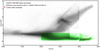 |
Fig. 1 Location of the search sample (GKM-type main-sequence stars, Teff < 6000 K, log[g/(cm s−2)] > 4.0) on the Hertzsprung-Russell diagram. The stellar parameters corresponding to the grey squares are obtained from the LAMOST-MRS parameter catalogue in the LAMOST DR8. The green crosses represent the sample for this study, and their parameters come from the LAMOST-MRS parameter catalogue in the LAMOST DR8 and DR9 v0. The red solid circles show the locations of the host stars for the three stellar CME candidates. |
Numbers of stars in our search sample.
2.3 CME Detection Method
In this study, we searched for stellar CME signals by examining the asymmetry of the Hα line. There are a number of techniques that can be used to analyse the asymmetries of line profiles (e.g. Tian et al. 2011; Maehara et al. 2021; Koller et al. 2021). In order to quickly and accurately select spectra with asymmetric Hα line profiles from the large sample, we designed a partition integral comparing method (PICM) to analyse each file. Each file comprises at least three continuously observed spectra for a target.
In the following, we describe the principle of the PICM. Panel A of Fig. 2 shows the Hα lines of the LAMOST-MRS spectra in a pre-processed file, which contains three continuously observed spectra. The exposure time of each spectrum is 1200 s. First, the blue region (6552.61–6564.61 Å) and the red region (6564.61–6576.61 Å) of the Hα line in each spectrum were respectively integrated:
 (1)
(1)
 (2)
(2)
 (3)
(3)
 (4)
(4)
In the above four equations, SB(n) and SR(n) are the integrals of the blue and red halves of the Hα line for each spectrum in a file, respectively. errB(n) and errR(n) are the corresponding errors. And N is the number of spectra in the file. Fnor is the normalized flux of the spectrum. σB(n) and σR(n) are the standard deviations of the normalized fluxes in the wavelength range of 6535–6545 Å and 6580–6590 Å, respectively. The integration limits for S B(n) and SR(n) are 12 Å, corresponding to a maximum Doppler velocity of 548 km s−1. For most of the detected CME candidates, their Hα profiles at least partially overlap with the integral regions. The disadvantage of this method is that very fast and very slow asymmetries may be missed when the CME-caused Hα profile is narrow.
We then calculated the absolute value of the difference between the integrals for each spectrum using the following formula:
 (5)
(5)
 (6)
(6)
When ∆Sn is greater than its corresponding error  , it indicates that the Hα line in the spectrum is asymmetric. As illustrated in panels B and C of Fig. 2, the maximum value of ∆Sn is represented by ∆Smax and the minimum value is represented by ∆Smin. In order to ensure that the asymmetric Hα profiles originate from the process of stellar eruption, rather than from the quiet stellar prominence, we further imposed the following requirement:
 (7)
(7)
If the Hα line profiles in a file satisfy the above conditions, the PICM will treat the file as a stellar CME candidate. Finally, we visually inspected the automatic search result to remove false stellar CME candidates caused by residual cosmic rays. In the meantime, we checked the SIMBAD database (Wenger et al. 2000) to ensure that each CME candidate comes from a late-type main-sequence single star, excluding the influence of eclipsing binaries, T Tauri stars, and RR Lyr stars.
After these processes, we detected three stellar CME candidates, and their related parameters are listed in Table 2. In Table 2, the first column, ‘LAMOST obsid’, provides the unique identification of each file in which a CME candidate was identified. The second column, ‘LAMOST designation’, gives the LAMOST name of the host star for each CME candidate. The third column provides the spectral type of the host stars, which is classified by the LAMOST 1D pipeline by matching the observed low-resolution spectrum with the templates (Luo et al. 2015). The uncertainty of the LAMOST spectral type is within two sub-classes. The fourth and fifth columns are the stellar effective temperature and surface gravity given by the LAMOST-MRS. The sixth and seventh columns are stellar parameters from the Two Micron All Sky Survey (2MASS), including the 2MASS designation and the J-band magnitude (Cutri et al. 2003). The last column is the stellar radius calculated from the relationship between the radius and spectral type for main-sequence stars (Cox 2000). The locations of the host stars of these three CME candidates on the Hertzsprung-Russell diagram are shown as the red solid circles in Fig. 1.
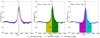 |
Fig. 2 Schematic diagram of the partition integral comparing method (PICM) for stellar CME detection. Panel A shows the Hα line profiles in a pre-processed file. Panels B and C show the maximum (∆Smax) and minimum values (∆Smin) of the ∆Sn, respectively. The ∆Sn is the absolute value of the difference between the integrals on the blue and red halves of each Hα profile. The vertical dotted black line represents the rest wavelength of the Hα line in each panel. |
Observation information and stellar parameters for the three CME candidates.
3 Results and Discussion
3.1 Stellar CME Candidate 1: LAMOST Obsid 876604049
3.1.1 Characteristics of the Chromospheric Lines in CME Candidate 1
The host star of CME candidate 1 (LAMOST obsid 876604049) is a main-sequence star (LAMOST J035012.86+242106.5). This host star is also named V371 Tau in the Pleiades. Several authors have confirmed that V371 Tau is a dwarf with a spectral type of M3Ve (Pesch 1961; Mirzoyan et al. 1990; Prosser et al. 1991; Parsamyan & Oganyan 1993). This star is also a flare star (Haro & Chavira 1970; Chavushian & Gharibjanian 1975; Haro et al. 1982; Mirzoyan et al. 1990; Parsamyan & Oganyan 1993; Hodgkin et al. 1995; Akopian 2001). There are four consecutively observed LAMOST-MRS spectra for CME candidate 1. Fig. 3 shows the pre-processed spectra of CME candidate 1 and two reference spectra of its host star. Following Koller et al. (2021), when the normalized spectra of the host star observed at different times are almost the same, these spectra are regarded as reference spectra. The first spectrum of CME candidate 1 is almost the same as the two reference spectra of the host star, indicating that this spectrum was also taken in the relatively quiet period. So we superimposed these three spectra and plotted them in Fig. 3. It can be seen from Fig. 3 that the intensities of the chromospheric lines (M g I triplet lines, Fe II 5170.47 Å, Hα, and He I 6680Å) in the second, third, and fourth spectra (solid orange, green, and red lines) of CME candidate 1 gradually increase, indicating the impulsive phase of a stellar flare. In order to analyse the asymmetries of the chromospheric lines in detail, we defined the following contrast profile:
 (8)
(8)
where Fnor,active (λ) is the normalized flux of an active spectrum in the CME candidate, and Fnor,ref(λ) is the normalized flux of the reference spectrum. The active spectrum and the reference spectrum were interpolated before this step. This operation allows these spectra to be compared at the same wavelengths. The contrast profile is often used to analyse asymmetric spectral line profiles observed during solar magnetic activity (Hong et al. 2014). For CME candidate 1, the first spectrum is a reference spectrum and has a S/N of 23 for the red arm and 8 for the blue arm. Therefore, this spectrum was selected as the reference spectrum and marked as ‘Reference spectrum’ in Fig. 3. The three Hα contrast profiles of the active spectra are shown in Fig. 4.
In this study, we performed double Gaussian fitting for the contrast profiles of the asymmetric chromospheric lines, the fitting function can be expressed as the following:
 (9)
(9)
In addition, we also defined the centre and maximum velocities of the two Gaussian components,
 (10)
(10)
 (11)
(11)
 (12)
(12)
 (13)
(13)
where λ0 is the centroid wavelength of a chromospheric line, c is the speed of light. The sign ‘±’ in Eqs. (11) and (13) is determined by the results of Eqs. (10) and (12), respectively. When the centroid velocity is negative, it is taken as ‘–’, otherwise it is taken as ‘+’. When the speed is negative, it means a blueshift. And when it is positive, it indicates a redshift.
The double Gaussian fitting results of the Hα contrast profiles of the three active spectra in CME candidate 1 are presented in Fig. 4. The fitting results reveal that there are two components in the Hα contrast profiles, one of which is the blueshifted component, as shown by the blue dashed lines in Fig. 4, and the other is the redshifted component shown by the green dashed lines. The amplitude and the full width at half maximum of these two components are gradually increasing. In addition, it can be seen from Fig. 5 that the central and maximum velocities of the blueshifted component both show a gradually increasing trend, while the central and maximum velocities of the redshifted component show a gradually decreasing trend.
For CME candidate 1, the S/N values of the red arms of the three active spectra are 25, 24, and 27, respectively. The values of the blue arms are 10, 9, and 11, respectively. Although the S/N of the blue arm is not as high as that of the red arm, it can be seen from the contrast profiles shown in Fig. 6 that the emission of the Mg I triplet lines gradually increases, and their blue wings also show obvious enhancements. Therefore, we also performed double Gaussian fitting for the contrast profiles of the Mg I triplet lines, and present the results in Fig. 6. The Fe II 5170.47 Å line emission can also be seen from Fig. 6 and its intensity gradually increases. Fig. 7 shows the centre and maximum velocities of the two components of the Mg I triplet lines. From panel A we can see that the components marked by the green dashed lines in Fig. 6 show a small redshift, with an average value of the central velocities around 5 km s−1. The panel B shows that their maximum velocities are decreasing. The components marked by the blue dashed lines in Fig. 6 reveal a blueshift. The average value of the centre velocities of these blueshifted components is about −70 km s−1 (panel C), and the average value of the maximum velocities is about −110 km s−1 (panel D). The single Gaussian fitting results for the He I 6680 Å contrast profiles are presented in Fig. 8. We can see that the Doppler shift is small and that the most obvious feature is the gradually increasing intensity.
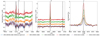 |
Fig. 3 Pre-processed spectra of CME candidate 1 (four solid lines) and the reference spectra of the host star (two dashed lines). Each spectrum is marked with the LAMOST local modified Julian day (LMJD) at the time of exposure. Panel A is part of the blue arm (5150–5200 Å), which contains the Mg I triplet lines (5168.94 Å, 5174.13 Å, and 5185.10 Å) and the Fe II 5170.47 Å line. The rest wavelengths of these chromospheric lines are marked with the vertical dotted black lines. Panel B is part of the red arm (6450–6700 Å), which contains the Hα (6564.61 Å) line and the He I 6680 Å line. The vacuum wavelengths of these lines are taken from van Hoof (2018). In panels A and B, the spectra of CME candidate 1 observed at different times are shifted on the vertical axis for a better illustration. In order to clearly show the changes in the Hα line profiles, the spectra near the Hα line are plotted in panel C. |
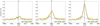 |
Fig. 4 Double Gaussian fitting results for the Hα contrast profiles of the three active spectra in CME candidate 1. The solid yellow lines are the Hα contrast profiles, and the solid red lines are the double Gaussian fitting results. The dashed blue and green lines represent the two Gaussian components. The vertical dotted black line indicates the rest wavelength of the Hα line in each panel. |
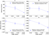 |
Fig. 5 Centre and maximum velocities of the two components in the Hα contrast profiles of the three active spectra in CME candidate 1. Panel A presents the centre velocities of the components shown by the dashed green lines in Fig. 4, and panel B shows the corresponding maximum velocities. Panel C presents the centre velocities of the components shown by the dashed blue lines in Fig. 4, and panel D shows the corresponding maximum velocities. The error bars represent the double Gaussian fitting errors. |
3.1.2 Asymmetries of the Chromospheric Lines in CME Candidate 1
The above analysis results indicate that CME candidate 1 is likely detected in the impulsive phase of the associated stellar flare. More importantly, the Mg I triplet lines and the Hα line show blue-wing enhancements at the same time. This is the first time that a blue-wing enhancement of Mg I triplet lines has been detected during a stellar flare. By checking the atomic line database (van Hoof 2018), no flare-related lines were found to appear in the blue wings of the Mg I triplet lines simultaneously. The S/N of the Hα is twice that of the Mg I triplet lines, and the centre velocity and maximum velocity of the blue-wing enhancement in Hα clearly show a gradually increasing trend. Therefore, the blue-wing enhancement could be interpreted as the line-of-sight projection of an outward moving stellar prominence (as part of a CME). The following is the basis of this interpretation.
First, Ding & Habbal (2017) observed the spectra of a solar CME associated with a prominence eruption during a total solar eclipse. Their spectra show an obvious emission in the Mg I triplet, Fe II and He I lines. The redshifts of these lines correspond to velocities ranging from under 100 to over 1500 km s−1. Blueshifts are rarely found in their lines. These observational results were interpreted as being caused by a solar CME moving away from the observer. The blue-wing enhancement of the spectral lines in our data may be caused by a CME propagating towards the observer. It should be noted that the blue-wing enhancement of the Mg I triplet lines is noisy and seems to be always separated from the line core. The corresponding velocities are small. Further observations are required to examine whether such features are CME-related.
Second, we want to determine if these blue-wing enhancements could be caused by the chromospheric evaporation. Solar flare observations show that signatures of chromospheric evaporation are often found in high-temperature lines, such as emission lines from the Fe XII–XXIV ions, while low-temperature chromospheric lines often do not reveal obvious blue-wing enhancements or blueshifts (e.g. Tian et al. 2014, 2015; Li & Ding 2011; Li et al. 2015b,a). In a solar flare observation, Tei et al. (2018) found that the Mg II h line shows a blue-wing enhancement in the impulsive phase of the flare. After using the cloud model to analyse the evolution of the Mg II h line profile during the flare, they suggested that the blue-wing enhancement of the Mg II h line may be caused by a scenario in which an upflow of cool plasma is lifted up by expanding hot plasma owing to the deep penetration of non-thermal electrons into the chromosphere. However, the maximum speed corresponding to the blue-wing enhancement of the Mg II h is only 14 km s−1, which is much smaller than that in our case. We noticed that the velocities of the blue-wing enhancement of the Mg I triplet lines and the Hα line in CME candidate 1 are different, which might be caused by the different S/N of these lines or the larger uncertainty of the Hα fitting. There is no obvious blue-wing enhancement in the Fe II 5170.47 Å and He i 6680 Å lines, which may be caused by the low S/N in these lines. However, the enhanced emission in both of these two spectral lines indicates that the host star is indeed in the process of an eruption.
The redshifted component in the Hα contrast profiles may be caused by chromospheric condensation. A solar flare observation reveals that the redshift of the Hα line caused by chromospheric condensation reaches 46 km s−1 before gradually decreasing (Tei et al. 2018). The decreasing velocity of the redshifted component of Hα in CME candidate 1 is similar to the result of Tei et al. (2018), and the centre velocity is close to the velocity of chro-mospheric condensation in the solar observation. The maximum velocity of the redshifted component in the Mg I triplet lines also shows a gradually decreasing trend. The central velocity shows a redshift that is smaller than that of Hα, which might be due to the different formation heights as well as S/N values of the Hα and Mg I triplet lines.
If the blue-wing enhancements of the Mg I triplet and Hα lines in CME candidate 1 are caused by a CME, we can select the strongest blue-wing enhancement of the Hα line to estimate the minimum mass of the CME through the following formula: (Houdebine et al. 1990; Koller et al. 2021):
 (14)
(14)
where R is the stellar radius, Femission is the integrated flux of the Hα blue-wing enhancement, and other parameters are specifically referred to Koller et al. (2021). Because the LAMOST-MRS only gives the relative flux of the spectrum, we calculated the Femission using the following method. We first integrated the enhancement area caused by the CME in the Hα contrast profile, denoted as QCME. This represents the ratio of the Hα enhancement caused by the CME to the quiet Hα flux, which can be calculated using the following equation:
 (15)
(15)
where Ac and σc are the amplitude and standard deviation of the blueshifted Gaussian component of the Hα contrast profile (blue dashed line in Fig. 4C), respectively. The quiet Hα flux (FHα,quiet) was calculated through the following empirical relationship:
 (16)
(16)
where χ is the ratio of the surface continuum flux (adjacent to the Hα line, FHα,con) to the stellar surface bolometric flux, which is given by Fang et al. (2018) when calculating the flux of Hα line in the LAMOST spectra. σ is the Stefan–Boltzmann constant.
Subsequently, we calculated the Femission through the following equation:
 (17)
(17)
Finally, the minimum mass of CME candidate 1 is estimated to be 4.12 × 10¹⁸ g, which is within the mass range of CME candidates for M dwarfs reported by Vida et al. (2019) and Maehara et al. (2021).
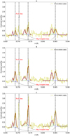 |
Fig. 6 Double Gaussian fitting results for the contrast profiles of the three active spectra in CME candidate 1. The vertical dotted black lines indicate the rest wavelengths of the Mg I triplet and Fe II 5170.47 Å lines. |
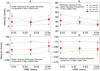 |
Fig. 7 Centre and maximum velocities of the two components in the contrast profiles of the Mg I triplet lines in CME candidate 1. Panel A presents the centre velocities of the components shown by the dashed green lines in Fig. 6, and panel B shows the corresponding maximum velocities. Panel C presents the centre velocities of the components shown by the dashed blue lines in Fig. 6, and panel D shows the corresponding maximum velocities. The solid blue, yellow, and green circles represent velocities of the Mg I triplet lines, respectively, and the red stars represent the corresponding average velocities. |
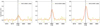 |
Fig. 8 Single Gaussian fitting results for the He I 6680 Å contrast profiles of the three active spectra in CME candidate 1. The solid red lines are the fitting results, and the vertical dotted black lines indicate the rest wavelength of the He I 6680 Å line. |
3.2 Stellar CME Candidate 2: LAMOST Obsid 635003103
The host star of CME candidate 2 (LAMOST obsid 635003103) is an M4-type main-sequence star (LAMOST J121933.15+015426.7). There are four consecutively observed LAMOST-MRS spectra for CME candidate 2. Fig. 9 shows the four pre-processed spectra. Although the Hα line profiles in the first three spectra appear to show a slight asymmetry, these three spectra are almost the same. We thus regarded these three spectra as reference spectra of the host star. The S/N values of the blue and red arms of the third spectrum are 7 and 15, respectively. They are both higher than those of the other two spectra. Thus, we chose the third spectrum as the reference spectrum and performed double Gaussian fitting for the Hα contrast profile of the active spectrum. The result is shown in Fig. 10. Panels A and B of Fig. 10 show that the Hα contrast profiles of the first two spectra reveal no obvious asymmetries. The double Gaussian fitting result in panel C shows that the Hα contrast profile exhibits a blueshifted component and a wide emission component centred around the rest wavelength of the Hα line. The centre velocity of the blueshifted component is −71 km s−1 and the maximum velocity is −151 km s−1. The blueshifted component in the Hα contrast profile may be caused by the projection of a CME eruption in the line of sight. Although its centre velocity is low, it is in the impulsive phase of the eruption and may continue to accelerate in the later stage, thereby perhaps escaping from the host star. The minimum mass of this possible CME is estimated to be 8.84 × 10¹⁷ g. The large line width of the broad emission component may result from the Stark broadening associated with the enhanced pressure by electrons (Švestka 1972; Zhu et al. 2019; Muheki et al. 2020a; Wu et al. 2022).
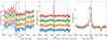 |
Fig. 9 Four pre-processed LAMOST-MRS spectra of CME candidate 2. The first three spectra (solid blue, orange, and green lines) are almost the same, and they are regarded as reference spectra of the host star. The three panels are similar to those in Fig. 3. |
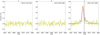 |
Fig. 10 Hα contrast profiles in CME candidate 2. Panels A and B show the Hα contrast profiles of the first two spectra. Panel C shows the double Gaussian fitting result for the Hα contrast profile of the active spectrum. |
3.3 Stellar CME Candidate 3: LAMOST Obsid 624510064
3.3.1 Characteristics of the Chromospheric Lines in CME Candidate 3
The host star of CME candidate 3 (LAMOST obsid 624510064) is an M2-type main-sequence star (LAMOST J041827.35+145813.6). There are three consecutively observed LAMOST-MRS spectra for CME candidate 3. Fig. 11 shows the three pre-processed spectra of CME candidate 3 and two reference spectra of the host star. We can see that the Hα emission in the active spectra gradually weakens and the red wing of Hα shows an obvious enhancement, possibly indicating the decay phase of a stellar flare. In addition, the Mg I triplet, Fe II 5170.47 Å and He I 6680 Å lines also exhibit emission. The double Gaussian fitting results for the Hα contrast profiles of the three active spectra in CME candidate 3 are shown in panels A, B, and C of Fig. 12. There are two redshifted components in the Hα contrast profiles, and both of their intensities gradually decrease. Fig. 13 shows that the centre and maximum velocities of the low-velocity component gradually decrease. The centre velocity of the high-velocity component shows a slightly increasing trend, but we realize that the fitting error is large. The maximum velocity gradually decreases and the largest velocity reaches 698 km s−1, which exceeds the surface escape velocity of the host star (552 km s−1). The single Gaussian fitting results for the He I 6680 Å contrast profiles are presented in panels D, E and F of Fig. 12, showing that the intensity and redshift of the He I line both gradually decrease. The He I line does not reveal two redshifted components as in the case of the Hα line, probably due to the lower S/N. Obvious emission and small redshifts can also be seen in the Mg I triplet and Fe II 5170.47 Å lines.
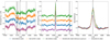 |
Fig. 11 Three pre-processed spectra of CME candidate 3 (three solid lines) and two reference spectra of the host star (two dashed lines). The three panels are similar to those in Fig. 3. |
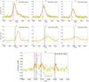 |
Fig. 12 Gaussian fitting results for the contrast profiles of the Hα, He I 6680 Å, and Mg I triplet lines in the active spectra of CME candidate 3. Panels A, B, and C are the results for Hα. The solid red lines are the double Gaussian fitting results, the dashed pink and green lines represent the two Gaussian components. Panels D, E, and F present the single Gaussian fitting results for the He I 6680 Å line, and the solid red lines are the fitting results. Panel G presents the single Gaussian fitting results for the Mg I triplet lines in the first active spectrum (solid blue line in Fig. 11). |
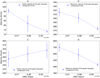 |
Fig. 13 Temporal evolution of the centre and maximum velocities of the two components in the Hα contrast profiles of the three active spectra for CME candidate 3. |
3.3.2 Doppler Shifts and Asymmetries of the Chromospheric Lines in CME Candidate 3
The high-speed redshifted component in panels A, B, and C of Fig. 12 (green) may be caused by a CME propagating in the direction away from the Earth, while the low-speed redshifted component (pink) likely results from coronal rain falling back to the stellar surface. The central velocity of the high-speed component shows a weak increasing trend. The average central velocity is 315 km s−1, and the largest value of the maximum velocities exceeds the surface escape velocity of the host star. Therefore, the high-speed component may be caused by a backward moving CME. A possible reason for the gradually decreasing maximum velocity is that as the CME expands during the propagation, the density of the outer region with a faster propagation speed decreases more, so its signal weakens in the line profiles. Another possible scenario is that the rapid propagation region of the CME is blocked by the star as the CME propagates away from the Earth, leaving just the slower-propagation region of the CME to be observed by the telescope. It should be noted that this may be a non-radial propagating CME occurring near the stellar limb, thus allowing both the flare and the backward propagating CME to be observed. Non-radial eruptions mean that CME motions deviate from the radial direction, often due to magnetic obstacles (coronal holes, helmet streamers, etc.) near the source regions of CMEs. Such a phenomenon is frequently observed on the Sun (Panasenco et al. 2013; Bi et al. 2013; Cécere et al. 2020). The trajectories of many solar non-radial eruptions deviate from radial propagation by around 30 degrees and some even reach 90 degrees (Filippov et al. 2001; Liewer et al. 2015; Yang et al. 2018). Based on the high-speed component shown in Fig. 12A, the minimum mass of the possible CME is estimated to be 1.85 × 10¹⁸ g.
The central and maximum velocities of the low-speed component gradually decrease, and the central velocities are lower than 100 km s−1. These characteristics are similar to those of the coronal rain on the Sun. A possible scenario is that one foot-point of the flare loop is located close to the stellar limb and the other footpoint is blocked by the stellar disk. In that case, cool coronal rain falling back to the stellar surface along the flare loop may result in a redshifted emission in the Hα. The typical speed of coronal rain is between 30 km s−1 and 150 km s−1 (Oliver et al. 2016; Antolin 2020; Li et al. 2021; Chen et al. 2022). In solar observations, redward asymmetries of the Hα line caused by coronal rain have been identified (Ahn et al. 2014). Fuhrmeister et al. (2018) analysed the Hα asymmetries of M dwarfs and suggested that a possible reason for the red-wing enhancement is coronal rain. Moreover, if this flare occurs near the stellar limb, the decrease of the emission in the Hα line core may be caused by the decreasing projected area of the flare ribbons as the star rotates. The observed redshifts of the Mg I triplet, Fe II 5170.47 Å and He 16680 Å lines may be caused by a combined effect of CME and coronal rain, which cannot be separated due to the low S/N in these spectral lines.
In order to verify the activity of the host star for CME candidate 3, we collected two sets of photometric data for the host star from the TESS database (Ricker et al. 2014,2015). After normalizing the flux and using the power spectral density to calculate the period of starspot activity, we plot these two sets of data in panels A and B in Fig. 14. Both sets of data show changes in the light curves caused by starspots, and the period of the spot activity is about 0.45 days. In addition, it can be seen from Fig. 14 that the host star produced multiple superflares during the two observation periods of the TESS. The light curve of the largest superflare is zoomed-in in panel C. The duration of this superflare is 58 minutes and its energy is estimated to be 4.37 × 1034 erg though a method used by Lu et al. (2019). The photometric data of the TESS suggests that the host star of CME candidate 3 is a very active star, which is likely to generate super-flares and CMEs to cause the Doppler shifts and asymmetries of the spectral lines, as mentioned above. For the host stars of the other two candidates, we were unable to collect other valuable data.
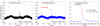 |
Fig. 14 TESS photometric data for the host star of CME candidate 3. Panel A shows the photometric data of TESS sector 5. The observation time is from November 15 to December 11, 2018. Several superflares are indicated by the pink arrows. Panel B shows the photometric data of TESS sector 32. Its observation time is from November 19 to December 17, 2020. The largest superflare in the TESS observation is marked by the red arrow. Panel C shows the zoomed-in version of the light curve of the largest superflare. ‘D’ and ‘E’ represent the flare duration and energy, respectively. |
Parameters of the three CME candidates.
4 Summary and Future Perspectives
In this work, we have searched for stellar CMEs on late-type main-sequence stars (Teff < 6000 K, log[g/(cm s−2)] > 4.0) in the LAMOST-MRS. The search sample contains 1379408 LAMOST-MRS spectra, which come from 226194 late-type main-sequence stars. By searching for the asymmetric Hα line profiles in the sample and conducting visual inspections, we identified three possible stellar CMEs. The relevant parameters of the three CME candidates are summarized in Table 3, including the CME mass, maximum bulk velocity, and maximum velocity. The host star of the three CME candidates are three M dwarfs. After performing a double Gaussian fitting for the Hα contrast profiles of the continuously observed spectra of the three CME candidates, we obtained the Doppler shifts of the asymmetric emission components. In light of the observations and theoretical models of solar flares and CMEs, the possible physical processes responsible for the asymmetric components of the Hα line profiles in the three CME candidates are discussed. The main results for these three stellar CME candidates are summarized as follows:
The host star of CME candidate 1 (LAMOST obsid 876604049) is an M1-type main-sequence star. This CME candidate appears to occur in the impulsive phase of the associated stellar flare, when intensities of the Mg I triplet, Fe II 5170.47 Å, Hα, and He I 6680 Å lines all gradually increase. The Mg I triplet and Hα lines exhibit obvious blue-wing enhancements, which are likely caused by a CME. The minimum mass of the CME is estimated to be 4.12 × 10¹⁸ g. The central and maximum velocities of the blue-wing component of Hα gradually increase. The Hα line also exhibits a redshifted component that is likely caused by the chromospheric condensation;
The host star of CME candidate 2 (LAMOST obsid 635003103) is an M4-type main-sequence star. The Hα line shows a blueshifted component that is likely caused by a CME. The minimum mass of the CME is estimated to be 8.84 × 10¹⁷ g. An additional broad emission component of the Hα line is probably caused by the Stark broadening effect;
The host star of CME candidate 3 (LAMOST obsid 624510064) is an M2-type main-sequence star. This CME candidate might occur in the decay phase of the associated stellar flare. The Hα line profiles show two redshifted components, one of which may be caused by a CME propagating in the direction away from the observer, and its minimum mass is estimated to be 1.85 × 10¹⁸ g. The other redshifted component may be caused by flare-triggered coronal rain. In addition, our analysis of the photometric TESS data shows that the host star of CME candidate 3 is a very active star, which is capable of generating superflares and CMEs and causing the asymmetries of the spectral lines.
From our large sample, we only detected three possible stellar CMEs. The probability of detecting stellar CMEs is much smaller than that of superflares (Maehara et al. 2012; Karoff et al. 2016) on late-type main-sequence stars. Koller et al. (2021) detected only six CME candidates among the 630 000 late-type main-sequence stars in SDSS. Muheki et al. (2020a) tried to search for stellar CMEs from 2000 high-dispersion spectra of AD Leo but did not find a CME candidate with a velocity exceeding the escape velocity of the host star. Vida et al. (2019) found 478 spectra with line asymmetries from 25 stars among about 5500 spectra and suggested that these 25 stars may show asymmetries in their spectral line profiles multiple times per day. The reason why Vida et al. (2019) detected more CME candidates may be due to a selection effect. Their samples are mainly active M dwarfs. Leitzinger et al. (2020) did not detect CME candidates in FGK-type main-sequence stars using the data sources that were partially similar to those of Vida et al. (2019). Therefore, the reason why there are fewer stellar CME candidates detected from our sample may be as follows. First, although the LAMOST-MRS has observed many spectra, the time-domain survey is in the early stage and the number of spectra observed for the same target is still too few. As the time-domain spectral survey continues, the LAMOST-MRS will conduct many more observations of stars, and we may find more stellar CMEs in the future. Second, the torus instability of magnetic flux ropes is one of the main triggering mechanisms of solar CMEs. On some stars, the background coronal magnetic field decreases slowly with altitude, which may suppress the torus instability and thus reduce the rate of stellar CME eruptions (Sun et al. 2022). The strong magnetic field on some stars may also suppress CME eruptions (Alvarado-Gómez et al. 2018; Li et al. 2020). In a word, the number of stellar CME candidates is still very small, and long-term continuous spectroscopic observations are highly desired to expand stellar CME samples.
Acknowledgements
This work is supported by the NSFC grants 12103004, 11825301 and 11790304, the fellowship of China National Postdoctoral Program for Innovative Talents (BX2021017), and the Strategic Priority Research Program of CAS (XDA17040507). We thank the referee and Professor Shenghong Gu for the very constructive suggestions and helpful comments. Guoshoujing Telescope (the Large Sky Area Multi-Object Fiber Spectroscopic Telescope LAMOST) is a National Major Scientific Project built by the Chinese Academy of Sciences. Funding for the project has been provided by the National Development and Reform Commission. LAMOST is operated and managed by the National Astronomical Observatories, Chinese Academy of Sciences. Part of the data in this paper was collected by the TESS mission and downloaded from the Mikulski Archive for Space Telescopes (MAST). This research has made use of the SIM-BAD database, operated at CDS, Strasbourg, France. This work uses the software TOPCAT (Taylor 2005).
References
- Aarnio, A. N., Matt, S. P., & Stassun, K. G. 2012, ApJ, 760, 9 [NASA ADS] [CrossRef] [Google Scholar]
- Abdul-Aziz, H., Abranin, E. P., Alekseev, I. Y., et al. 1995, A&As, 114, 509 [NASA ADS] [Google Scholar]
- Abranin, E. P., Bazelyan, L. L., Alekseev, I. Y., et al. 1997, Ap&SS, 257, 131 [NASA ADS] [CrossRef] [Google Scholar]
- Abranin, E. P., Alekseev, I. Y., Avgoloupis, S., et al. 1998, Astron. Astrophys. Trans., 17, 221 [NASA ADS] [CrossRef] [Google Scholar]
- Ahn, K., Chae, J., Cho, K.-S., et al. 2014, Sol. Phys., 289, 4117 [NASA ADS] [CrossRef] [Google Scholar]
- Airapetian, V. S., Danchi, W. C., Dong, C. F., et al. 2018, ArXiv e-prints [arXiv:1801.07333] [Google Scholar]
- Akopian, A. A. 2001, Astrophysics, 44, 106 [NASA ADS] [CrossRef] [Google Scholar]
- Alvarado-Gómez, J. D., Drake, J. J., Cohen, O., Moschou, S. P., & Garraffo, C. 2018, ApJ, 862, 93 [Google Scholar]
- Antolin, P. 2020, Plasma Phys. Controlled Fusion, 62, 014016 [Google Scholar]
- Argiroffi, C., Reale, F., Drake, J. J., et al. 2019, Nat. Astron., 3, 742 [NASA ADS] [CrossRef] [Google Scholar]
- Benz, A. O., & Güdel, M. 2010, ARA&A, 48, 241 [NASA ADS] [CrossRef] [Google Scholar]
- Bi, Y., Jiang, Y., Yang, J., et al. 2013, ApJ, 773, 162 [NASA ADS] [CrossRef] [Google Scholar]
- Boiko, A. I., Konovalenko, A. A., Koliadin, V. L., & Melnik, V. N. 2012, Adv. Astron. Space Phys., 2, 121 [Google Scholar]
- Bond, H. E., Mullan, D. J., O’Brien, M. S., & Sion, E. M. 2001, ApJ, 560, 919 [Google Scholar]
- Cao, D., Gu, S., Ge, J., et al. 2019, MNRAS, 482, 988 [NASA ADS] [CrossRef] [Google Scholar]
- Cécere, M., Sieyra, M. V., Cremades, H., et al. 2020, Adv. Space Res., 65, 1654 [CrossRef] [Google Scholar]
- Chavushian, H. S., & Gharibjanian, A. T. 1975, Astrophysics, 11, 565 [NASA ADS] [Google Scholar]
- Chen, P. F. 2011, Living Rev. Solar Phys., 8, 1 [NASA ADS] [CrossRef] [Google Scholar]
- Chen, H., Tian, H., Li, L., et al. 2022, A&A, 659, A107 [NASA ADS] [CrossRef] [EDP Sciences] [Google Scholar]
- Cox, A. N. 2000, Allen’s astrophysical quantities [Google Scholar]
- Crosley, M. K., & Osten, R. A. 2018, ApJ, 862, 113 [NASA ADS] [CrossRef] [Google Scholar]
- Crosley, M. K., Osten, R. A., Broderick, J. W., et al. 2016, ApJ, 830, 24 [NASA ADS] [CrossRef] [Google Scholar]
- Cui, X.-Q., Zhao, Y.-H., Chu, Y.-Q., et al. 2012, Res. Astron. Astrophys., 12, 1197 [Google Scholar]
- Cutri, R. M., Skrutskie, M. F., van Dyk, S., et al. 2003, VizieR Online Data Catalog: II/246 [Google Scholar]
- Deng, L.-C., Newberg, H. J., Liu, C., et al. 2012, Res. Astron. Astrophys., 12, 735 [Google Scholar]
- Ding, A., & Habbal, S. R. 2017, ApJ, 842, L7 [NASA ADS] [CrossRef] [Google Scholar]
- Fang, X.-S., Zhao, G., Zhao, J.-K., & Bharat Kumar, Y. 2018, MNRAS, 476, 908 [NASA ADS] [CrossRef] [Google Scholar]
- Filippov, B. P., Gopalswamy, N., & Lozhechkin, A. V. 2001, Sol. Phys., 203, 119 [NASA ADS] [CrossRef] [Google Scholar]
- Forbes, T. G. 2000, J. Geophys. Res., 105, 23153 [Google Scholar]
- Franciosini, E., Pallavicini, R., & Tagliaferri, G. 2001, A&A, 375, 196 [NASA ADS] [CrossRef] [EDP Sciences] [Google Scholar]
- Fuhrmeister, B., & Schmitt, J. H. M. M. 2004, A&A, 420, 1079 [NASA ADS] [CrossRef] [EDP Sciences] [Google Scholar]
- Fuhrmeister, B., Czesla, S., Schmitt, J. H. M. M., et al. 2018, A&A, 615, A14 [NASA ADS] [CrossRef] [EDP Sciences] [Google Scholar]
- Gopalswamy, N., Yashiro, S., Michalek, G., et al. 2009, Earth, Moon and Planets, 104, 295 [NASA ADS] [CrossRef] [Google Scholar]
- Gopalswamy, N., Akiyama, S., Yashiro, S., & Mäkelä, P. 2010, in Astrophysics and Space Science Proceedings, Magnetic Coupling between the Interior and Atmosphere of the Sun, 19, 289 [NASA ADS] [Google Scholar]
- Guenther, E. W., & Emerson, J. P. 1997, A&A, 321, 803 [NASA ADS] [Google Scholar]
- Gunn, A. G., Doyle, J. G., Mathioudakis, M., Houdebine, E. R., & Avgoloupis, S. 1994, A&A, 285, 489 [NASA ADS] [Google Scholar]
- Haisch, B. M., Linsky, J. L., Bornmann, P. L., et al. 1983, ApJ, 267, 280 [NASA ADS] [CrossRef] [Google Scholar]
- Haro, G., & Chavira, E. 1970, Bol. Observ. Tonantzintla Tacubaya, 5, 23 [NASA ADS] [Google Scholar]
- Haro, G., Chavira, E., & Gonzalez, G. 1982, Bol. Inst. Tonantzintla, 3, 3 [NASA ADS] [Google Scholar]
- Harrison, R. A. 1996, Sol. Phys., 166, 441 [NASA ADS] [CrossRef] [Google Scholar]
- Hodgkin, S. T., Jameson, R. F., & Steele, I. A. 1995, MNRAS, 274, 869 [NASA ADS] [CrossRef] [Google Scholar]
- Hong, J., Ding, M. D., Li, Y., Fang, C., & Cao, W. 2014, ApJ, 792, 13 [NASA ADS] [CrossRef] [Google Scholar]
- Houdebine, E. R., Foing, B. H., & Rodono, M. 1990, A&A, 238, 249 [NASA ADS] [Google Scholar]
- Karoff, C., Knudsen, M. F., De Cat, P., et al. 2016, Nat. Commun., 7, 11058 [NASA ADS] [CrossRef] [Google Scholar]
- Khodachenko, M. L., Ribas, I., Lammer, H., et al. 2007, Astrobiology, 7, 167 [CrossRef] [Google Scholar]
- Kilpua, E., Koskinen, H. E. J., & Pulkkinen, T. I. 2017, Living Rev. Solar Phys., 14, 5 [NASA ADS] [CrossRef] [Google Scholar]
- Koller, F., Leitzinger, M., Temmer, M., et al. 2021, A&A, 646, A34 [NASA ADS] [CrossRef] [EDP Sciences] [Google Scholar]
- Korhonen, H., Vida, K., Leitzinger, M., Odert, P., & Kovács, O. E. 2017, in Living Around Active Stars, eds. D. Nandy, A. Valio, & P. Petit, 328, 198 [NASA ADS] [Google Scholar]
- Lammer, H., Lichtenegger, H. I. M., Kulikov, Y. N., et al. 2007, Astrobiology, 7, 185 [NASA ADS] [CrossRef] [Google Scholar]
- Leitzinger, M., Odert, P., Hanslmeier, A., et al. 2009, in American Institute of Physics Conference Series, 15th Cambridge Workshop on Cool Stars, Stellar Systems, and the Sun, ed. E. Stempels, 1094, 680 [NASA ADS] [CrossRef] [Google Scholar]
- Leitzinger, M., Odert, P., Ribas, I., et al. 2011, A&A, 536, A62 [NASA ADS] [CrossRef] [EDP Sciences] [Google Scholar]
- Leitzinger, M., Odert, P., Greimel, R., et al. 2014, MNRAS, 443, 898 [NASA ADS] [CrossRef] [Google Scholar]
- Leitzinger, M., Odert, P., Greimel, R., et al. 2020, MNRAS, 493, 4570 [Google Scholar]
- Li, Y., & Ding, M. D. 2011, ApJ, 727, 98 [NASA ADS] [CrossRef] [Google Scholar]
- Li, D., Ning, Z. J., & Zhang, Q. M. 2015a, ApJ, 813, 59 [Google Scholar]
- Li, Y., Ding, M. D., Qiu, J., & Cheng, J. X. 2015b, ApJ, 811, 7 [NASA ADS] [CrossRef] [Google Scholar]
- Li, T., Hou, Y., Yang, S., et al. 2020, ApJ, 900, 128 [NASA ADS] [CrossRef] [Google Scholar]
- Li, L., Peter, H., Chitta, L. P., & Song, H. 2021, ApJ, 910, 82 [CrossRef] [Google Scholar]
- Liewer, P., Panasenco, O., Vourlidas, A., & Colaninno, R. 2015, Sol. Phys., 290, 3343 [Google Scholar]
- Lin, J., Raymond, J. C., & van Ballegooijen, A. A. 2004, ApJ, 602, 422 [NASA ADS] [CrossRef] [Google Scholar]
- Linsky, J. 2019, Host Stars and their Effects on Exoplanet Atmospheres, 955 [Google Scholar]
- Liu, N., Fu, J.-N., Zong, W., et al. 2019, Res. Astron. Astrophys., 19, 075 [CrossRef] [Google Scholar]
- Liu, C., Fu, J., Shi, J., et al. 2020, ArXiv e-prints [arXiv:2005.07210] [Google Scholar]
- Lu, H.-P., Zhang, L.-Y., Shi, J., et al. 2019, ApJS, 243, 28 [NASA ADS] [CrossRef] [Google Scholar]
- Luo, A. L., Zhao, Y.-H., Zhao, G., et al. 2015, Res. Astron. Astrophys., 15, 1095 [Google Scholar]
- Maehara, H., Shibayama, T., Notsu, S., et al. 2012, Nature, 485, 478 [NASA ADS] [Google Scholar]
- Maehara, H., Notsu, Y., Namekata, K., et al. 2021, PASJ, 73, 44 [NASA ADS] [CrossRef] [Google Scholar]
- Mirzoyan, L. V., Hambarian, V. V., & Garigjanian, A. T. 1990, Astrofizika, 33, 5 [NASA ADS] [Google Scholar]
- Moschou, S.-P., Drake, J. J., Cohen, O., Alvarado-Gomez, J. D., & Garraffo, C. 2017, ApJ, 850, 191 [NASA ADS] [CrossRef] [Google Scholar]
- Moschou, S.-P., Drake, J. J., Cohen, O., et al. 2019, ApJ, 877, 105 [NASA ADS] [CrossRef] [Google Scholar]
- Muheki, P., Guenther, E. W., Mutabazi, T., & Jurua, E. 2020a, A&A, 637, A13 [NASA ADS] [CrossRef] [EDP Sciences] [Google Scholar]
- Muheki, P., Guenther, E. W., Mutabazi, T., & Jurua, E. 2020b, MNRAS, 499, 5047 [NASA ADS] [CrossRef] [Google Scholar]
- Namekata, K., Maehara, H., Honda, S., et al. 2021, Nat. Astron., 6, 241 [Google Scholar]
- Oliver, R., Soler, R., Terradas, J., & Zaqarashvili, T. V. 2016, ApJ, 818, 128 [Google Scholar]
- Ottmann, R., & Schmitt, J. H. M. M. 1996, A&A, 307, 813 [NASA ADS] [Google Scholar]
- Panasenco, O., Martin, S. F., Velli, M., & Vourlidas, A. 2013, Sol. Phys., 287, 391 [Google Scholar]
- Pandey, J. C., & Singh, K. P. 2012, MNRAS, 419, 1219 [NASA ADS] [CrossRef] [Google Scholar]
- Parsamyan, E. S., & Oganyan, G. B. 1993, Astrofizika, 36, 501 [NASA ADS] [Google Scholar]
- Pesch, P. 1961, ApJ, 133, 1085 [NASA ADS] [CrossRef] [Google Scholar]
- Pritchard, J., Murphy, T., Zic, A., et al. 2021, MNRAS, 502, 5438 [NASA ADS] [CrossRef] [Google Scholar]
- Prosser, C. F., Stauffer, J., & Kraft, R. P. 1991, AJ, 101, 1361 [NASA ADS] [CrossRef] [Google Scholar]
- Ricker, G. R., Winn, J. N., Vanderspek, R., et al. 2014, SPIE Conf. Ser., 9143, 914320 [Google Scholar]
- Ricker, G. R., Winn, J. N., Vanderspek, R., et al. 2015, J. Astron. Telescopes Instrum. Syst., 1, 014003 [Google Scholar]
- Segura, A., Walkowicz, L. M., Meadows, V., Kasting, J., & Hawley, S. 2010, Astrobiology, 10, 751 [Google Scholar]
- Sun, X., Török, T., & DeRosa, M. L. 2022, MNRAS, 509, 5075 [Google Scholar]
- Švestka, Z. 1972, Sol. Phys., 24, 154 [CrossRef] [Google Scholar]
- Taylor, M. B. 2005, in Astronomical Society of the Pacific Conference Series, Astronomical Data Analysis Software and Systems XIV, eds. P. Shopbell, M. Britton, & R. Ebert, 347, 29 [NASA ADS] [Google Scholar]
- Tei, A., Sakaue, T., Okamoto, T. J., et al. 2018, PASJ, 70, 100 [NASA ADS] [CrossRef] [Google Scholar]
- Tian, H., McIntosh, S. W., De Pontieu, B., et al. 2011, ApJ, 738, 18 [NASA ADS] [CrossRef] [Google Scholar]
- Tian, H., McIntosh, S. W., Xia, L., He, J., & Wang, X. 2012, ApJ, 748, 106 [NASA ADS] [CrossRef] [Google Scholar]
- Tian, H., Li, G., Reeves, K. K., et al. 2014, ApJ, 797, L14 [Google Scholar]
- Tian, H., Young, P. R., Reeves, K. K., et al. 2015, ApJ, 811, 139 [NASA ADS] [CrossRef] [Google Scholar]
- Tsuboi, Y., Koyama, K., Murakami, H., et al. 1998, ApJ, 503, 894 [NASA ADS] [CrossRef] [Google Scholar]
- van Hoof, P. A. M. 2018, Galaxies, 6, 63 [NASA ADS] [CrossRef] [Google Scholar]
- Veronig, A. M., Odert, P., Leitzinger, M., et al. 2021, Nat. Astron., 5, 697 [NASA ADS] [CrossRef] [Google Scholar]
- Vida, K., Kriskovics, L., Oláh, K., et al. 2016, A&A, 590, A11 [NASA ADS] [CrossRef] [EDP Sciences] [Google Scholar]
- Vida, K., Leitzinger, M., Kriskovics, L., et al. 2019, A&A, 623, A49 [NASA ADS] [CrossRef] [EDP Sciences] [Google Scholar]
- Wang, R., Luo, A. L., Chen, J. J., et al. 2019, ApJS, 244, 27 [NASA ADS] [CrossRef] [Google Scholar]
- Wang, R., Luo, A. L., Chen, J.-J., et al. 2020, ApJ, 891, 23 [Google Scholar]
- Wang, J., Xin, L. P., Li, H. L., et al. 2021, ApJ, 916, 92 [NASA ADS] [CrossRef] [Google Scholar]
- Webb, D. F., & Howard, T. A. 2012, Living Rev. Solar Phys., 9, 3 [NASA ADS] [CrossRef] [Google Scholar]
- Wenger, M., Ochsenbein, F., Egret, D., et al. 2000, A&As, 143, 9 [NASA ADS] [CrossRef] [EDP Sciences] [Google Scholar]
- Wu, Y., Chen, H., Tian, H., et al. 2022, ApJ, 928, 180 [NASA ADS] [CrossRef] [Google Scholar]
- Xu, Y., Tian, H., Hou, Z., et al. 2022, ApJ, 931, 76 [NASA ADS] [CrossRef] [Google Scholar]
- Yang, J., Dai, J., Chen, H., Li, H., & Jiang, Y. 2018, ApJ, 862, 86 [CrossRef] [Google Scholar]
- Yang, Z., Tian, H., Bai, X., et al. 2022, ApJS, 260, 36 [NASA ADS] [CrossRef] [Google Scholar]
- Yelle, R., Lammer, H., & Ip, W.-H. 2008, Space Sci. Rev., 139, 437 [Google Scholar]
- Zhang, B., Li, J., Yang, F., et al. 2021, ApJS, 256, 14 [NASA ADS] [CrossRef] [Google Scholar]
- Zhao, G., Zhao, Y.-H., Chu, Y.-Q., Jing, Y.-P., & Deng, L.-C. 2012, Res. Astron. Astrophys., 12, 723 [NASA ADS] [CrossRef] [Google Scholar]
- Zhu, Y., Kowalski, A. F., Tian, H., et al. 2019, ApJ, 879, 19 [NASA ADS] [CrossRef] [Google Scholar]
- Zong, W., Fu, J.-N., De Cat, P., et al. 2020, ApJS, 251, 15 [NASA ADS] [CrossRef] [Google Scholar]
All Tables
All Figures
|
Fig. 1 Location of the search sample (GKM-type main-sequence stars, Teff < 6000 K, log[g/(cm s−2)] > 4.0) on the Hertzsprung-Russell diagram. The stellar parameters corresponding to the grey squares are obtained from the LAMOST-MRS parameter catalogue in the LAMOST DR8. The green crosses represent the sample for this study, and their parameters come from the LAMOST-MRS parameter catalogue in the LAMOST DR8 and DR9 v0. The red solid circles show the locations of the host stars for the three stellar CME candidates. |
| In the text | |
|
Fig. 2 Schematic diagram of the partition integral comparing method (PICM) for stellar CME detection. Panel A shows the Hα line profiles in a pre-processed file. Panels B and C show the maximum (∆Smax) and minimum values (∆Smin) of the ∆Sn, respectively. The ∆Sn is the absolute value of the difference between the integrals on the blue and red halves of each Hα profile. The vertical dotted black line represents the rest wavelength of the Hα line in each panel. |
| In the text | |
|
Fig. 3 Pre-processed spectra of CME candidate 1 (four solid lines) and the reference spectra of the host star (two dashed lines). Each spectrum is marked with the LAMOST local modified Julian day (LMJD) at the time of exposure. Panel A is part of the blue arm (5150–5200 Å), which contains the Mg I triplet lines (5168.94 Å, 5174.13 Å, and 5185.10 Å) and the Fe II 5170.47 Å line. The rest wavelengths of these chromospheric lines are marked with the vertical dotted black lines. Panel B is part of the red arm (6450–6700 Å), which contains the Hα (6564.61 Å) line and the He I 6680 Å line. The vacuum wavelengths of these lines are taken from van Hoof (2018). In panels A and B, the spectra of CME candidate 1 observed at different times are shifted on the vertical axis for a better illustration. In order to clearly show the changes in the Hα line profiles, the spectra near the Hα line are plotted in panel C. |
| In the text | |
|
Fig. 4 Double Gaussian fitting results for the Hα contrast profiles of the three active spectra in CME candidate 1. The solid yellow lines are the Hα contrast profiles, and the solid red lines are the double Gaussian fitting results. The dashed blue and green lines represent the two Gaussian components. The vertical dotted black line indicates the rest wavelength of the Hα line in each panel. |
| In the text | |
|
Fig. 5 Centre and maximum velocities of the two components in the Hα contrast profiles of the three active spectra in CME candidate 1. Panel A presents the centre velocities of the components shown by the dashed green lines in Fig. 4, and panel B shows the corresponding maximum velocities. Panel C presents the centre velocities of the components shown by the dashed blue lines in Fig. 4, and panel D shows the corresponding maximum velocities. The error bars represent the double Gaussian fitting errors. |
| In the text | |
|
Fig. 6 Double Gaussian fitting results for the contrast profiles of the three active spectra in CME candidate 1. The vertical dotted black lines indicate the rest wavelengths of the Mg I triplet and Fe II 5170.47 Å lines. |
| In the text | |
|
Fig. 7 Centre and maximum velocities of the two components in the contrast profiles of the Mg I triplet lines in CME candidate 1. Panel A presents the centre velocities of the components shown by the dashed green lines in Fig. 6, and panel B shows the corresponding maximum velocities. Panel C presents the centre velocities of the components shown by the dashed blue lines in Fig. 6, and panel D shows the corresponding maximum velocities. The solid blue, yellow, and green circles represent velocities of the Mg I triplet lines, respectively, and the red stars represent the corresponding average velocities. |
| In the text | |
|
Fig. 8 Single Gaussian fitting results for the He I 6680 Å contrast profiles of the three active spectra in CME candidate 1. The solid red lines are the fitting results, and the vertical dotted black lines indicate the rest wavelength of the He I 6680 Å line. |
| In the text | |
|
Fig. 9 Four pre-processed LAMOST-MRS spectra of CME candidate 2. The first three spectra (solid blue, orange, and green lines) are almost the same, and they are regarded as reference spectra of the host star. The three panels are similar to those in Fig. 3. |
| In the text | |
|
Fig. 10 Hα contrast profiles in CME candidate 2. Panels A and B show the Hα contrast profiles of the first two spectra. Panel C shows the double Gaussian fitting result for the Hα contrast profile of the active spectrum. |
| In the text | |
|
Fig. 11 Three pre-processed spectra of CME candidate 3 (three solid lines) and two reference spectra of the host star (two dashed lines). The three panels are similar to those in Fig. 3. |
| In the text | |
|
Fig. 12 Gaussian fitting results for the contrast profiles of the Hα, He I 6680 Å, and Mg I triplet lines in the active spectra of CME candidate 3. Panels A, B, and C are the results for Hα. The solid red lines are the double Gaussian fitting results, the dashed pink and green lines represent the two Gaussian components. Panels D, E, and F present the single Gaussian fitting results for the He I 6680 Å line, and the solid red lines are the fitting results. Panel G presents the single Gaussian fitting results for the Mg I triplet lines in the first active spectrum (solid blue line in Fig. 11). |
| In the text | |
|
Fig. 13 Temporal evolution of the centre and maximum velocities of the two components in the Hα contrast profiles of the three active spectra for CME candidate 3. |
| In the text | |
|
Fig. 14 TESS photometric data for the host star of CME candidate 3. Panel A shows the photometric data of TESS sector 5. The observation time is from November 15 to December 11, 2018. Several superflares are indicated by the pink arrows. Panel B shows the photometric data of TESS sector 32. Its observation time is from November 19 to December 17, 2020. The largest superflare in the TESS observation is marked by the red arrow. Panel C shows the zoomed-in version of the light curve of the largest superflare. ‘D’ and ‘E’ represent the flare duration and energy, respectively. |
| In the text | |
Current usage metrics show cumulative count of Article Views (full-text article views including HTML views, PDF and ePub downloads, according to the available data) and Abstracts Views on Vision4Press platform.
Data correspond to usage on the plateform after 2015. The current usage metrics is available 48-96 hours after online publication and is updated daily on week days.
Initial download of the metrics may take a while.