| Issue |
A&A
Volume 695, March 2025
|
|
|---|---|---|
| Article Number | L2 | |
| Number of page(s) | 9 | |
| Section | Letters to the Editor | |
| DOI | https://doi.org/10.1051/0004-6361/202452857 | |
| Published online | 25 February 2025 | |
Letter to the Editor
A filament eruption on the RS CVn-type star UX Ari
1
Yunnan Observatories, Chinese Academy of Sciences, Kunming 650216, China
2
Key Laboratory for the Structure and Evolution of Celestial Objects, Chinese Academy of Sciences, Kunming 650216, China
3
International Centre of Supernovae, Yunnan Key Laboratory, Kunming 650216, China
4
School of Astronomy and Space Science, University of Chinese Academy of Sciences, Beijing 101408, China
⋆ Corresponding authors; This email address is being protected from spambots. You need JavaScript enabled to view it.
; This email address is being protected from spambots. You need JavaScript enabled to view it.
Received:
4
November
2024
Accepted:
31
January
2025
Abstract
Context. Stellar flares can be accompanied by filament or prominence eruptions, which may lead to stellar coronal mass ejections (CMEs) that have significant impacts on surrounding exoplanets and stellar evolution.
Aims. We report the capture of a filament eruption associated with an optical flare on the RS CVn-type star UX Ari.
Methods. Based on high-resolution spectroscopic observations, we investigated the Doppler-shifted absorption features appeared in the Hα flaring spectra, which can be indicative of a filament eruption.
Results. A huge optical flare was observed, which lasted for at least 150 hours and released an energy of about 1.47 × 1037 erg in the Hα line. The corresponding bolometric white-light energy is converted to be 1.03 × 1039 erg, indicating that the flare is comparable to the most intense stellar superflares. A blueshifted absorption feature with a bulk velocity of −143.9 km s−1 emerged in the Hα line region during the initial phase of the flare, which then decelerated and turned into redshifted absorption. This suggests that a filament eruption happened and ultimately fell back toward the star, suggesting that it represents a failed filament eruption. The erupted filament mass of 8.5 − 15.0 × 10²⁰ g and the kinetic energy of 8.8 − 15.5 × 1034 erg are derived. Furthermore, the relationship between the filament eruption and the flare is likely characterized by a sympathetic eruption.
Key words: Sun: coronal mass ejections (CMEs) / Sun: filaments / prominences / stars: chromospheres / stars: coronae / stars: flare
© The Authors 2025
 Open Access article, published by EDP Sciences, under the terms of the Creative Commons Attribution License (https://creativecommons.org/licenses/by/4.0), which permits unrestricted use, distribution, and reproduction in any medium, provided the original work is properly cited.
This article is published in open access under the Subscribe to Open model. This email address is being protected from spambots. You need JavaScript enabled to view it. to support open access publication.
1. Introduction
Solar flares can be accompanied by filament eruptions (also known as prominence eruptions when viewed on the solar limb) and coronal mass ejections (CMEs), all of which have significant impacts on space weather (Forbes 2000; Koleva et al. 2021). Stellar superflares (with energies of 1033–1038 erg; Schaefer et al. 2000) have been frequently observed on cool stars, particularly in the surveys conducted by the Kepler space telescope (e.g., Maehara et al. 2012) and the Transiting Exoplanet Survey Satellite (TESS; e.g., Tu et al. 2020; Yang et al. 2023). Superflares may be associated with the production of much larger CMEs, which may affect the potential habitability of the surrounding exoplanets (Airapetian et al. 2016; Cherenkov et al. 2017) and contribute significantly to mass and angular momentum losses during stellar evolution (Aarnio et al. 2012).
In the solar case, eruptive filaments or prominences are commonly believed to form the CME cores in frequently observed three-part structures of solar CMEs (Forbes 2000). Consequently, stellar filament and prominence eruptions can be indirect evidence of stellar CMEs, and its investigation may also be an effective means of obtaining information on formation and evolution of stellar CMEs in lower coronae.
The detection of Doppler-shifted absorption and emission signatures in chromospheric line profiles provides one way to search for stellar filament and prominence eruptions and potential CMEs. Currently, there have been some such observational cases on cool stars (e.g., Houdebine et al. 1990; Vida et al. 2019; Koller et al. 2021; Namekata et al. 2021; Wu et al. 2022; Lu et al. 2022; Inoue et al. 2023; Cao & Gu 2024; Namekata et al. 2024). Among these cases, only one eruptive filament had been detected on the young solar-type star EK Dra (Namekata et al. 2021), and a CME is probably associated with the eruption.
UX Ari (also known as HD 21242 or BD+28°532) is a non-eclipsing spectroscopic binary system, consisting of a K0 IV primary star and a G5 V secondary, with an orbital period of about 6.44 days. UX Ari is a highly active RS CVn-type star. Its K0 IV primary component shows significant starspot activity and strong chromospheric emission in the Hα, Ca II H & K, and Ca II IRT lines. In addition, UX Ari is also a high-rate flaring star, exhibiting flares several times in a wide range of wavelengths (Simon et al. 1980; Elias et al. 1995; Montes et al. 1996; Franciosini et al. 2001; Gu et al. 2002; Richards et al. 2003; Cao & Gu 2017; Kurihara et al. 2024). This indicates that UX Ari may have frequent filament and prominence eruptions and CMEs based on the close association between solar CMEs and energetic flares.
This study focuses on a filament eruption that occurred during the initial phase of a huge optical flare on UX Ari. In Sect. 2 we provide details of the observations, data reduction, and spectral subtraction of chromospheric lines. A huge optical flare and analysis of the flaring spectra are described in Sect. 3, and the filament eruption is discussed in Sect. 4. In Sect. 5 we conclude and summarize the new results.
2. Observations, data reduction, and spectral subtraction
Spectroscopic observations of UX Ari were obtained by using the fiber-fed high-resolution spectrograph (HRS) installed on the 2.16 m telescope at the Xinglong station of the National Astronomical Observatories, Chinese Academy of Sciences, China in 2017–2018 (Fan et al. 2016). HRS produces spectra with a resolving power of R = λ/Δλ ≃ 48 000 in a wavelength range of 3900–10 000 Å, using a 4096 × 4096 pixel CCD detector. The detailed observing information is listed in Table A.1.
The data were reduced with the IRAF1 package, following the prescription in Cao & Gu (2024). Moreover, the telluric lines that appeared in the chromospheric lines were removed by using a telluric template derived from the spectrum of the rapidly rotating early-type star HR 8858 (B5 V, v sin i = 316 km s−1).
To separate the pure activity contribution from the observed line profiles, we applied the spectral subtraction technique with the STARMOD program (Barden 1985; Montes et al. 1997, 2000). More details can be found in Appendix A.
3. Analysis and results
3.1. A huge optical flare event
A long-duration optical flare was looked for in the observations from 2017 December 28 (HJD = 2458116) to 2018 January 3 (HJD = 2458122), during which the Hα and other chromospheric lines showed stronger emission. In particular, the He I D3 line, which is typically used as a flare indicator due to its high excitation potential (e.g., Zirin 1988; Gu et al. 2002; Cao et al. 2019; Cao & Gu 2024), exhibited obvious emission features (see Fig. A.1). Figure 1a shows the equivalent widths (EWs) of the STARMOD-subtracted Hα spectra plotted against HJD. It should be noted that the Hα subtractions contain both intrinsic chromospheric emission and flare radiation. Therefore, we removed the intrinsic chromospheric emission from the subtractions to obtain the pure flare radiation. The intrinsic chromospheric emission intensity was obtained by averaging the EWs of two subtracted Hα spectra, respectively observed on 2017 December 8 (HJD = 2458096) and 9 (HJD = 2458097). These two spectra were obtained at comparable phases to the spectra on 2017 December 28, with no flare radiation shown in the spectra (hereafter pre-flare reference spectra; see Fig. B.1). The EWs removed the intrinsic chromospheric emission are shown in Fig. 1b, where we set the observing time (HJD = 2458116.083) as zero point and then derived the flare time (see the top axis). It shows that the flare reached its maximum intensity at about 75 hours, and that the flare event lasted for at least 150 hours.
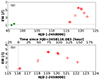 |
Fig. 1. Temporal variation of the EWs of the Hα line. (a) EWs of the subtracted Hα spectra plotted against HJD. The dotted line represents the intrinsic chromospheric emission level. (b) EWs removed the intrinsic chromospheric emission, plotted against HJD and flare time. The dotted line indicates the zero point of the flare time. |
Since the K0 IV primary star is very active in UX Ari and the subtracted emission is associated with this star during the flare event (see Fig. A.1), it can be concluded that the optical flare occurred on this star. The flare energy released in the Hα line is estimated to be about 1.47 × 1037 erg (see the calculation procedure in Appendix C). Moreover, based on the relationship between the Hα and bolometric white-light flare energy from Eq. (2) of Namekata et al. (2024), the bolometric white-light flare radiation energy is derived to be 1.03 × 1039 erg, which suggests that this optical flare is comparable to the most intense stellar superflares.
3.2. Hα line profiles during the flare event
3.2.1. Doppler-shifted absorption feature
As shown in Fig. 2a, five spectra were observed on 2017 November 28 during the initial phase of the flare event. It is evident that the Hα spectra displayed variable profiles. The first spectrum showed a pronounced absorption in the blue wing, while both the central region and red wing exhibited more intense emission. Furthermore, as illustrated in Fig. 2b, when compared with the synthesized spectrum, an excess absorption feature emerged in its blue wing. For the pre-flare reference spectra, there were no similar absorption features (see Fig. B.1), providing stronger support for the detection of a blueshifted excess absorption feature.
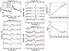 |
Fig. 2. Hα spectra on 2017 December 28 and Doppler-shifted absorption features in the profiles. (a) Observed Hα spectra overlaid for comparison. (b) Observed (solid lines) and synthesized (dash-dotted gray lines) Hα spectra. For the last four observed spectra (solid colored lines), the first observed spectrum is superimposed for comparison. Arrows indicate the absorption features that appeared in the Hα profiles. (c) Subtracted Hα profiles and Gaussian fitting (dashed lines) for the subtraction at phase 0.703. (d) Differences between the first observed Hα spectrum and the subsequent four observed spectra (black solid lines), together with the Gaussian fittings (dashed lines). Phases and flare times are indicated in the panels, and all spectra are corrected to the rest velocity frame of the K0 IV primary star of UX Ari. (e) Temporal variation of the bulk velocities of the absorption feature. The blue and red dashed lines represent the linear fittings for the blueshifted and redshifted velocities, respectively. The gray dotted line indicates the zero-point of the velocity. (f) Temporal variation of the EWs of the absorption feature. |
In comparison, it can be seen from Fig. 2a and b that the second spectrum did not show a similar enhanced absorption feature in the blue wing and failed to exhibit the anticipated stronger emission in the central region of the line profile compared with the first spectrum during the rising phase of the flare. The observed weaker emission cannot be attributed to a weakening of the flare intensity since other chromospheric activity indicators, such as the He I D3 and Ca IIλ8542 lines (see Fig. D.1), did not show decreased emission at this time. A plausible explanation for this discrepancy is that the excess absorption feature observed in the blue wing of the first spectrum underwent a wavelength shift in the second spectrum. This shift resulted in localized absorption in the line profile, leading to a weaker central emission and producing a redshifted fake excess emission at a velocity of about 150 km s−1. In the third spectrum, the central emission exhibited an increased intensity relative to the second spectrum, accompanied by a more redshifted fake emission feature in the red wing. This could be attributed to the further redshift of the excess absorption feature, which not only resulted in a more redshifted emission feature, but also promoted the recovery and enhancement of the central emission. Furthermore, the variable profiles observed in the final two spectra further supported the detection of a continuous redshift of the excess absorption feature. In summary, the variable Hα profiles doubtlessly revealed a rapidly Doppler-shifted excess absorption feature moving from the blue wing to the red wing.
With the Hα subtraction obtained at phase 0.703, illustrated in Fig. 2c, we employed the Gaussian fitting method to model the profile and a Gaussian absorption profile was used to represent the excess absorption feature. For the other four subtracted Hα spectra, because the absorption feature is completely mixed with the subtracted emission, it was difficult to apply the same modeling method. Therefore, we used the first spectrum as a reference and individually subtracted each of the last four observed Hα spectra from it to extract the absorption feature. The differences are shown in Fig. 2d and modeled using the Gaussian fitting method. As in the previous description, the variations observed in the line profiles of the last four spectra are mainly attributed to the localized absorption feature that had shifted to the central regions and red wings of these spectral profiles. Moreover, this excess absorption appeared in the blue wing of the first profile. Therefore, it was appropriate to use the first profile as a reference, particularly its emission region, to isolate the absorption features presented in the last four profiles. Although this approach may not accurately determine the intensity of the absorption feature, it can provide information regarding its velocity variation. In addition, the presence of excess absorption in the blue wing of the first profile results in a localized stronger emission feature in each difference spectrum. In contrast, weaker emission was also obtained in the last three difference spectra, resulting from changes in the line profiles, particularly their central regions that evolved into stronger emission. The fitting results indicate that the absorption feature first appeared with a velocity of −143.9 km s−1 at phase 0.703, then decelerated to −1.1 km s−1 at phase 0.722, next turned into a redshifted absorption, and finally moved to 49.2 km s−1 at phase 0.731 over the course of about 4.4 hours. The velocities and EWs of the absorption features are plotted against flare time in Figs. 2e and f, respectively.
3.2.2. Far-redshifted excess emission features
For the observations on 2017 December 31 and 2018 January 1 and 3, there are far-redshifted emission components in the fitted Hα subtractions, indicating the presence of other forms of plasma motion during the flare (see more details in Appendix E).
4. Discussion
4.1. A filament eruption during the initial phase of the flare
4.1.1. Rapidly Doppler-shifted absorption feature indicating a failed filament eruption
The blueshifted absorption feature with a bulk velocity of −143.9 km s−1 implies the existence of low-temperature and high-density neutral plasma above the stellar disk that is moving toward the observer at a higher velocity. A filament eruption is a reliable explanation. A similar absorption feature resulting from a filament eruption connected to a superflare had also been found by Namekata et al. (2021) on a young solar-type star EK Dra, and further verified by analyzing a solar filament eruption with the Sun-as-a-star method. For our situation, the bulk velocity of the blueshifted absorption is much smaller than the escape velocity of the K0 IV primary star of UX Ari. The escape velocity is estimated to be 304 km s−1 from  km s−1 with the mass M⋆ = 1.3 M⊙ and the radius R⋆ = 5.6 R⊙ (Hummel et al. 2017). Moreover, even when a projection angle of 45° is assumed, the velocity (∼−204 km s−1) is still far below the escape velocity, which suggests that the erupted filament was unable to escape from the star and also indicates that the filament would fall back to the star.
The blueshifted absorption feature decelerated to −1.1 km s−1 at phase 0.722, implying that the filament nearly erupted to its highest point at this phase. The average deceleration rate from phase 0.703–0.722 is approximately 13.6 m s−2, which exceeds the deceleration of about 11.5 m s−2 due to the surface gravity of the K0 IV primary star (log g = 3.06 cm s−2, Hummel et al. 2017). This suggests that an additional force was influencing the filament eruption in addition to the gravity. The strong magnetic field on UX Ari can account for this additional force because the erupted filament might be suppressed by the strong overlying magnetic field of the active star (see Alvarado-Gómez et al. 2018). The erupted filament could reach a minimum height of about 7.5 × 10⁵ km (∼0.19 stellar radii of K0 IV) based on the deceleration rate.
After phase 0.722, the absorption feature became accelerated redshift (see Fig. 2e), suggesting that the erupted filament material was falling back toward the star, and it is also consistent with the previous point of view that the filament would eventually fall back to the star. The average acceleration rate during the falling phase was about 9.4 m s−2, which is slightly less than the value of the surface gravity. This indicates that the angle between the filament’s falling direction and the line of sight is relatively insignificant. Therefore, a projection angle of about 35° is derived from i = arccos(9.4/11.5) when the filament is subjected to gravity and falling. This also implies that the previous assumption of 45° for the projection angle is reasonable.
To sum up, a filament eruption occurred during our observations. The filament showed a gradual decrease in the eruption velocity, then reached its highest point, and finally fell back toward the star. Therefore, this is indicative of a failed filament eruption. Although the filament eruption occurred during the initial phase of the flare, the spectral line had already exhibited an increase in intensity prior to this event. Therefore, it is challenging to definitively conclude that the filament eruption was responsible for triggering the flare. However, it remains possible that the filament had already begun to become unstable before the flare.
4.1.2. Properties of the filament eruption
The filament mass is derived to be 8.5 − 15.0 × 10²⁰ g (see Appendix F), which is consistent with the masses of the erupted prominences detected on other active stars (e.g., Inoue et al. 2023; Cao & Gu 2024). Moreover, the kinetic energy is derived to be 8.8 − 15.5 × 1034 erg. Figures 3a and b show the mass and kinetic energy as functions of the flare energy emitted in the GOES X-ray and bolometric flare energy in comparison with solar filament and prominence eruptions and CMEs. The prescription for conversion of the flare energy can be found in Cao & Gu (2024). It can be seen that the erupted filament mass is basically consistent with the prediction of the solar flare-CME relation, indicating that the filament eruption has an underlying mechanism that is similar to solar eruptions. This result is in good agreement with the properties of filament and prominence eruptions found on other active stars (e.g., Moschou et al. 2019; Namekata et al. 2021; Inoue et al. 2023; Cao & Gu 2024; Namekata et al. 2024). Moreover, similar to findings on other active stars, the kinetic energy is lower than that expected from solar CMEs. One potential explanation, as discussed in the previous section, is that the overlying magnetic field on UX Ari could suppress the filament eruption, and this could result in the low kinetic energy. Another probable reason is that inner filament or prominence eruptions typically exhibit lower velocities than outer hotter CME plasmas, as observed on the Sun. However, it is important to note that the kinetic energy derived by us is 4–5 orders of magnitude lower than that predicted by the solar observations, and is also significantly lower than that observed on other stars. Typically, the kinetic energies are about two orders of magnitude lower than that predicted from the solar extrapolation on other active stars (Moschou et al. 2019), and there are also some studies that had reported kinetic energies consistent with the solar flare-CME relation (e.g., Inoue et al. 2023). For the significantly lower kinetic energy, there might be other contributing factors, such as the possible occurrence of a sympathetic eruption (see discussion in Sect. 4.2).
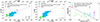 |
Fig. 3. Mass MCME (a) and kinetic energy Ek (b) plotted as functions of flaring bolometric energy (bottom horizontal axis) and X-ray energy emitted in the GOES band (top axis) for solar and stellar filament and prominence eruptions and CMEs. The solar CME data (filled sky-blue circles) are derived from Yashiro & Gopalswamy (2009). The solar prominence and filament eruptions and surges (green plus signs) are from Namekata et al. (2024), originally taken from Namekata et al. (2021) and Kotani et al. (2023). The dashed and dotted lines are trend fits for the solar CMEs expressed as |

Although erupted filaments or prominences finally return to the Sun, CMEs can still occur. Namekata et al. (2021) suggested that a CME happened on EK Dra through comparing the length scale and velocity of the filament eruption with those of solar filament eruptions. The same method is adopted here, as shown in Fig. 3c, where the length scale and velocity of the filament eruption on UX Ari is compared with those of solar eruptions. It can be seen that the filament eruption of UX Ari is above the threshold, which can determine whether a filament eruption is associated with a CME or not. This suggests that the filament eruption on UX Ari may be associated with a CME. Nevertheless, this conclusion is still questionable since the threshold is derived from solar observations. EK Dra is a Sun-like star, so the threshold may be potentially applicable. The magnetic field strength and topology of UX Ari, as well as its atmospheric parameters, are different from those of the Sun and the scale of the filament eruption is considerably larger than that observed on the Sun (see Fig. 3). These discrepancies may imply that the threshold is not applicable here. Therefore, as we cannot draw any conclusions for this point, we leave it as an open question to future follow-up studies.
4.2. Potential flaring location and its possible spatial relationship with the filament eruption
The broad emission component in the subtracted flaring spectra is dominant, and its Doppler-shifted velocity ranges approximately from −19 to 20 km s−1 over phases from 0.012 to 0.649, spanning more than half of the period. This suggests that the Doppler shift of the broad emission component is likely attributable to the stellar rotation. A cosine function is utilized to model the velocity variation, resulting in a maximum blueshifted velocity of about −25 km s−1 on HJD = 2458118.285 (at phase 0.045). This occurs when the flare was located at the stellar limb that is moving toward us. Moreover, the highest blueshifted velocity and the v sin i value of 39 km s−1 for the K0 IV primary star imply that the flare occurred at a latitude of about 50° (∼arccos(25/39)). The inclination of UX Ari is about 59.2° (Duemmler & Aarum 2001), which implies that the regions of the photosphere located above latitude of 59.2° are consistently visible. Because the flare ribbon occurred in the chromosphere, which is higher than the photosphere, it is possible that the flare happened at a latitude of about 50°, and thus is always visible.
The filament eruption took place on the hemisphere oriented toward us on 2017 December 28, whereas the flare was located at the opposing hemisphere (see Fig. E.2a). Therefore, if the filament eruption originated from the flare with a highly inclined trajectory relative to the vertical direction, the inclination angle would exceed 90°. Although solar filament eruptions can occasionally occur at significantly inclined angles (Seki et al. 2019), no instances of such extreme inclination angles have been found in solar observations. Alternatively, another possible scenario is that the filament eruption and the flare, although they occur nearly at the same time, were located at different regions. In solar observations, some successive eruption events that occur at different active regions may be physically interconnected. This phenomenon is referred to as sympathetic eruptions, wherein the occurrence of one eruption event triggers another at a different location (Wheatland et al. 1998). Therefore, for our situation, the relationship between the filament eruption and the flare may be indicative of a sympathetic eruption.
5. Summary and conclusions
A huge optical flare event was detected on the active RS CVn-type star UX Ari, with a duration of at least 150 hours. The flare energy released in the Hα line is estimated to be about 1.47 × 1037 erg, and the bolometric white-light flare energy is converted to be 1.03 × 1039 erg. A rapidly Doppler-shifted absorption feature moving from the blue wing of the Hα line profile to the red wing was identified during the initial phase of the flare, which can be ascribed to a filament eruption. The filament finally fell back toward the star, and therefore it is a possible failed filament eruption. The erupted filament mass of 8.5 − 15.0 × 10²⁰ g and the kinetic energy of 8.8 − 15.5 × 1034 erg are derived. The mass value is in good agreement with the solar flare-CME relation. However, the value of kinetic energy is significantly lower than that predicted by this relation. Furthermore, the relationship between the filament eruption and the flare is likely characterized by a sympathetic eruption.
Data availability
The reduced spectra are available at the CDS via anonymous ftp to cdsarc.cds.unistra.fr (130.79.128.5) or via https://cdsarc.cds.unistra.fr/viz-bin/cat/J/A+A/695/L2
IRAF is distributed by the National Optical Astronomy Observatories, which is operated by the Association of Universities for Research in Astronomy (AURA), Inc., under cooperative agreement with the National Science Foundation.
Acknowledgments
The authors thank the anonymous referee for the careful review and helpful suggestions, which lead to a significant improvement in our manuscript. The authors would like to express their gratitude to the staff of the Xinglong 2.16m telescope for their assistance and support. This work is partially supported by the Open Project Program of the Key Laboratory of Optical Astronomy, National Astronomical Observatories, Chinese Academy of Sciences. The present study is also financially supported by the National Natural Science Foundation of China (NSFC) under grant Nos. 10373023, 10773027, 11333006, and U1531121, the Yunnan Fundamental Research Projects (grant Nos. 202201AT070186 and 202305AS350009), the Yunnan Revitalization Talent Support Program (Young Talent Project), and International Centre of Supernovae, Yunnan Key Laboratory (No. 202302AN360001). The authors also acknowledge the science research grant from the China Manned Space Project.
References
- Aarnio, A. N., Matt, S. P., & Stassun, K. G. 2012, ApJ, 760, 9 [NASA ADS] [CrossRef] [Google Scholar]
- Aarum Ulvås, V., & Henry, G. W. 2003, A&A, 402, 1033 [NASA ADS] [CrossRef] [EDP Sciences] [Google Scholar]
- Airapetian, V. S., Glocer, A., Gronoff, G., Hébrard, E., & Danchi, W. 2016, Nature Geoscience, 9, 452 [NASA ADS] [CrossRef] [Google Scholar]
- Alvarado-Gómez, J. D., Drake, J. J., Cohen, O., Moschou, S. P., & Garraffo, C. 2018, ApJ, 862, 93 [Google Scholar]
- Barden, S. C. 1985, ApJ, 295, 162 [NASA ADS] [CrossRef] [Google Scholar]
- Cao, D., & Gu, S. 2024, ApJ, 963, 13 [Google Scholar]
- Cao, D., Gu, S., Ge, J., et al. 2019, MNRAS, 482, 988 [NASA ADS] [CrossRef] [Google Scholar]
- Cao, D.-T., & Gu, S.-H. 2017, Research in Astronomy and Astrophysics, 17, 055 [NASA ADS] [CrossRef] [Google Scholar]
- Cherenkov, A., Bisikalo, D., Fossati, L., & Möstl, C. 2017, ApJ, 846, 31 [Google Scholar]
- Drake, J. J., Cohen, O., Yashiro, S., & Gopalswamy, N. 2013, ApJ, 764, 170 [NASA ADS] [CrossRef] [Google Scholar]
- Duemmler, R., & Aarum, V. 2001, A&A, 370, 974 [NASA ADS] [CrossRef] [EDP Sciences] [Google Scholar]
- Elias, N. M., I, Quirrenbach, A., Witzel, A., et al. 1995, ApJ, 439, 983 [NASA ADS] [CrossRef] [Google Scholar]
- Fan, Z., Wang, H., Jiang, X., et al. 2016, PASP, 128, 115005 [NASA ADS] [CrossRef] [Google Scholar]
- Forbes, T. G. 2000, J. Geophys. Res., 105, 23153 [Google Scholar]
- Franciosini, E., Pallavicini, R., & Tagliaferri, G. 2001, A&A, 375, 196 [NASA ADS] [CrossRef] [EDP Sciences] [Google Scholar]
- Fuhrmeister, B., Czesla, S., Schmitt, J. H. M. M., et al. 2018, A&A, 615, A14 [NASA ADS] [CrossRef] [EDP Sciences] [Google Scholar]
- Gu, S. H., Tan, H. S., Shan, H. G., & Zhang, F. H. 2002, A&A, 388, 889 [NASA ADS] [CrossRef] [EDP Sciences] [Google Scholar]
- Hall, J. C. 1996, PASP, 108, 313 [NASA ADS] [CrossRef] [Google Scholar]
- Houdebine, E. R., Foing, B. H., & Rodono, M. 1990, A&A, 238, 249 [NASA ADS] [Google Scholar]
- Hummel, C. A., Monnier, J. D., Roettenbacher, R. M., et al. 2017, ApJ, 844, 115 [NASA ADS] [CrossRef] [Google Scholar]
- Inoue, S., Maehara, H., Notsu, Y., et al. 2023, ApJ, 948, 9 [Google Scholar]
- Koleva, K., Dechev, M., & Duchlev, P. 2021, Journal of Atmospheric and Solar-Terrestrial Physics, 212, 105464 [NASA ADS] [CrossRef] [Google Scholar]
- Koller, F., Leitzinger, M., Temmer, M., et al. 2021, A&A, 646, A34 [NASA ADS] [CrossRef] [EDP Sciences] [Google Scholar]
- Kotani, Y., Shibata, K., Ishii, T. T., et al. 2023, ApJ, 943, 143 [NASA ADS] [CrossRef] [Google Scholar]
- Kurihara, M., Iwakiri, W. B., Tsujimoto, M., et al. 2024, ApJ, 965, 135 [NASA ADS] [CrossRef] [Google Scholar]
- Lu, H.-P., Tian, H., Zhang, L.-Y., et al. 2022, A&A, 663, A140 [NASA ADS] [CrossRef] [EDP Sciences] [Google Scholar]
- Maehara, H., Shibayama, T., Notsu, S., et al. 2012, Nature, 485, 478 [NASA ADS] [Google Scholar]
- Mein, P., & Mein, N. 1988, A&A, 203, 162 [Google Scholar]
- Montes, D., Fernández-Figueroa, M. J., De Castro, E., et al. 2000, A&AS, 146, 103 [NASA ADS] [CrossRef] [EDP Sciences] [Google Scholar]
- Montes, D., Fernandez-Figueroa, M. J., de Castro, E., & Sanz-Forcada, J. 1997, A&AS, 125, 263 [NASA ADS] [CrossRef] [EDP Sciences] [Google Scholar]
- Montes, D., Sanz-Forcada, J., Fernandez-Figueroa, M. J., & Lorente, R. 1996, A&A, 310, L29 [NASA ADS] [Google Scholar]
- Moschou, S.-P., Drake, J. J., Cohen, O., et al. 2019, ApJ, 877, 105 [NASA ADS] [CrossRef] [Google Scholar]
- Namekata, K., Maehara, H., Honda, S., et al. 2021, Nature Astronomy, 6, 241 [NASA ADS] [CrossRef] [Google Scholar]
- Namekata, K., Airapetian, V. S., Petit, P., et al. 2024, ApJ, 961, 23 [Google Scholar]
- Richards, M. T., Waltman, E. B., Ghigo, F. D., & Richards, D. S. P. 2003, ApJS, 147, 337 [NASA ADS] [CrossRef] [Google Scholar]
- Schaefer, B. E., King, J. R., & Deliyannis, C. P. 2000, ApJ, 529, 1026 [NASA ADS] [CrossRef] [Google Scholar]
- Seki, D., Otsuji, K., Ishii, T., et al. 2019, Sun and Geosphere, 14, 95 [NASA ADS] [Google Scholar]
- Seki, D., Otsuji, K., Ishii, T. T., Asai, A., & Ichimoto, K. 2021, Earth. Planets and Space, 73, 58 [NASA ADS] [CrossRef] [Google Scholar]
- Simon, T., Linsky, J. L., & Schiffer, F. H., I 1980, ApJ, 239, 911 [NASA ADS] [CrossRef] [Google Scholar]
- Tu, Z.-L., Yang, M., Zhang, Z. J., & Wang, F. Y. 2020, ApJ, 890, 46 [NASA ADS] [CrossRef] [Google Scholar]
- Vida, K., Leitzinger, M., Kriskovics, L., et al. 2019, A&A, 623, A49 [NASA ADS] [CrossRef] [EDP Sciences] [Google Scholar]
- Wang, J., Li, H. L., Xin, L. P., et al. 2022, ApJ, 934, 98 [NASA ADS] [CrossRef] [Google Scholar]
- Wheatland, M. S., Sturrock, P. A., & McTiernan, J. M. 1998, ApJ, 509, 448 [NASA ADS] [CrossRef] [Google Scholar]
- Wu, Y., Chen, H., Tian, H., et al. 2022, ApJ, 928, 180 [NASA ADS] [CrossRef] [Google Scholar]
- Yang, Z., Zhang, L., Meng, G., et al. 2023, A&A, 669, A15 [NASA ADS] [CrossRef] [EDP Sciences] [Google Scholar]
- Yashiro, S., & Gopalswamy, N. 2009, in Universal Heliophysical Processes, eds, N. Gopalswamy, & F. Webb, 257, 233 [NASA ADS] [Google Scholar]
- Zirin, H. 1988, Astrophysics of the Sun (Cambridge: Cambridge Univ. Press) [Google Scholar]
Appendix A: Observing log of UX Ari and spectral subtraction
Table A.1 presents the observing log of UX Ari, which includes the observing date, exposure time (Exp. time), heliocentric Julian date (HJD), and orbital phase calculated with the ephemeris HJD = 2, 456, 238.134 + 6.437888P from Hummel et al. (2017). The zero phase corresponds to the time when the G5 V secondary component is at inferior conjunction in front of the K0 IV primary component. The long-duration optical flare was observed from 2017 December 28 to 2018 January 3, while the observations on 2017 December 8 and 9 were used to obtain the intrinsic chromospheric emission during the flare.
Observing information for UX Ari.
Spectral subtraction technique has been widely used for chromospheric activity studies in active binary systems. The STARMOD program can construct a synthesized spectrum through artificially rotationally broadening, intensity weighting, and radial velocity shifting for the spectra of the reference inactive stars with the similar spectral types and luminosity classes as the two components of the binary system. Subsequently, this synthesized spectrum is subtracted from the observed spectrum of the binary system. The synthesized spectrum represents the non-active state of the system, and therefore the subtraction between the observed and synthesized spectra comes from the pure activity. The activity contribution can be obtained by measuring equivalent widths (EWs) of the subtracted line profiles. For our situation, the spectra of two inactive stars HR 3351 (K0 IV) and HR 3309 (G5 V) are used as references for the K0 IV primary and G5 V secondary star of UX Ari, respectively. The vsini values of 39 km s−1 for the primary component and 7.5 km s−1 for the secondary component are used, and the intensity weight ratios of two components are 0.74/0.26 for the Hα spectral region and 0.69/0.31 for the He I D3 spectral region (Cao & Gu 2017). As examples, we show the chromospheric lines of one spectrum and illustrate the above described processing in Fig. A.1.
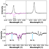 |
Fig. A.1. Examples of the observed, synthesized, and subtracted spectra for the Hα (upper panel) and He I D3 line (lower panel) spectral regions in one flaring spectrum obtained at phase 0.322 on 2018 January 1. For the left part of each panel, the black solid line is the observed spectrum, and the magenta dashed line represents the synthesized spectrum. “P” and “S" indicate the primary and secondary components of UX Ari, respectively. The resulting subtraction spectrum is displayed in the right part. The label identifying each chromospheric line is also marked. |
Appendix B: Pre-flare reference spectra
The pre-flare reference spectra observed on 2017 December 8 (HJD = 2458096) and 9 (HJD = 2458097) are shown in Fig. B.1, in comparison with the synthesized spectra. Moreover, for two Hα subtractions of the pre-flare reference spectra after removing the synthesized spectra, we also calculate a mean spectrum and compared it with the subtracted flaring spectra in the figure.
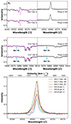 |
Fig. B.1. Same as Fig. A.1, but for the spectra observed at phase 0.626 on 2017 December 8 and at phase 0.767 on 2017 December 9 (upper and middle panel, respectively). The mean subtracted Hα spectrum (gray dash-dotted line) is obtained for the two subtractions and plotted together with the subtracted flaring spectra in the bottom panel. For each observing night, one subtracted flaring spectrum is presented as an example. All subtracted spectra are corrected to the rest velocity frame of the K0 IV primary star of UX Ari. |
When analyzing the spectral line profiles, we do not subtract the per-flare reference spectra from the observed flaring spectra. The reason is that UX Ari is a highly active RS CVn-type star, so that its chromospheric line profile can vary significantly among different nights. A gap of some days existed between the observation of the pre-flare reference spectra and that of the flaring spectra. Consequently, we only opted to use the pre-flare reference spectra to determine the intrinsic chromospheric emission intensity during the flare.
Appendix C: Calculation of the flare energy released in the Hα line
For our situation, a few observations were made per night during the flare and therefore we calculate a mean EW for the flare emission in each observing night. We compute the stellar continuum flux FHα (in erg cm−2 s−1 Å−1) near the Hα line region as a function of the color index B − V (∼ 0.88 for UX Ari; Aarum Ulvås & Henry 2003) based on the empirical relationship
![Mathematical equation: $$ \begin{aligned} \log {F_{H{\alpha }}}=[7.538-1.081(B-V)]\pm {0.33}\nonumber \\ 0.0~\le ~B-V~\le ~1.4 \end{aligned} $$](/articles/aa/full_html/2025/03/aa52857-24/aa52857-24-eq4.gif) (C.1)
(C.1)
from Hall (1996), and then convert the mean EW into an absolute surface flux FS (in erg cm−2 s−1). The EW value is corrected to the total continuum before converting to the absolute surface flux. Therefore, the mean flare luminosity per observing night is obtained by using the derived absolute surface flux and the stellar radius R⋆ = 5.6 R⊙ (Hummel et al. 2017) of the K0 IV primary star.
To estimate the flare energy, we integrate the mean luminosity by 48 hours for the observation on 2017 December 28 and 24 hours for the other observations, and then add them together. Because there is an observing gap between 2017 December 28 and December 30, the integrating time of 48 hours is used for the observation on December 28. Therefore, the flare energy released in the Hα line is estimated to be about 1.47 × 1037 erg.
Appendix D: Observed He I D3 and Ca IIλ8542 lines on 2017 December 28
Figure D.1 presents the observed He I D3 and Ca IIλ8542 line profiles on 2017 December 28, demonstrating progressively enhanced emission features consistent with the expected variation during the rising phase of the stellar flare.
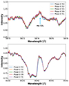 |
Fig. D.1. Observed He I D3 (upper panel) and Ca IIλ8542 (bottom panel) line profiles on 2017 December 28. The velocities of all spectra are corrected relative to the K0 IV primary star of UX Ari. |
Appendix E: Far-redshifted emission components
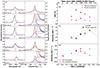 |
Fig. E.1. Hα spectra from 2017 December 30 to 2018 January 3. (a) Examples of Gaussian fitting for the Hα subtractions. Left part: Observed (black solid lines) and synthesized (magenta dashed lines) Hα spectra. The observing dates and phases are also marked. Right part: Gaussian fitting (colored dashed lines) for the Hα subtractions (black solid lines). All subtracted spectra are corrected to the rest velocity frame of the K0 IV primary star of UX Ari. The insets show zoomed-in images of the spectral ranges with the far-redshifted emission components. (b) Temporal variations of the EWs of the narrow and broad emission components. (c) Temporal variations of the velocities of the broad emission component and the fitting line. (d) Temporal variations of the velocities of the far-redshifted emission component and the G5 V secondary component relative to the K0 IV primary component. |
For the flaring spectra observed from 2017 December 30 to 2018 January 3, the subtracted Hα profiles are also modeled using the Gaussian fitting method. The Hα profiles usually can be well fitted by a narrow emission component and a broad emission one. As displayed in Fig. E.1 (a), one spectrum from each night’s observation is presented as an example. In Fig. E.1 (b) and (c), the EWs of the narrow and broad emission components and the velocities of the broad emission component are respectively plotted against HJD and flare time. It can be seen that the broad emission component is dominant and Doppler-shifted. Additionally, for the observations on 2017 December 31 and 2018 January 1 and 3, there are far-redshifted emission components in the fitted profiles. These components exhibit bulk velocities of about 170 km s−1, 250 km s−1, and 250 km s−1, respectively. The velocities of the far-redshifted emission components are plotted against HJD and flare time in Fig. E.1 (d), and the velocities of the G5 V secondary component relative to the K0 IV primary component are also plotted. It can be found that these far-redshifted emission components are not associated with the G5 V secondary component (see Fig. E.1 (d)). Furthermore, the flaring spectra exhibited broader profiles compared to the subtracted pre-flare reference spectra (see Fig. B.1). Consequently, these far-redshifted emissions can be attributed to plasma motions associated with the flare event.
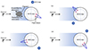 |
Fig. E.2. Schematic diagram that expresses the interpretation of the Doppler-shifted excess absorptions and the possible flaring location. Panel (a) represents the occurrence of the Doppler-shifted absorption features observed on 2017 December 28 and the flaring location at that time. Panels (b), (c), and (d) depict the possible flaring location on 2017 December 31, 2018 January 1, and 2018 January 3, respectively. The dashed circles represent the latitude of 50°. The small telescope illustration is from Fig. 7 in Inoue et al. (2023). |
As discussed in Sect. 4.2, the flare region was located at the stellar limb that is moving toward us at phase 0.045. Taking further account of the orbital motion of UX Ari, the flaring location at a different orbital phase can be inferred and a schematic diagram illustrating the potential flaring location is presented in Fig. E.2. For the observation on 2017 December 28, we can infer that the flare was located at the hemisphere nearly opposite to that of the filament eruption (Fig. E.2 (a)). By 2017 December 31, the star had rotated approximately 44° from phase 0.045. Consequently, the flare region shifted to a location similar to that shown in Fig. E.2 (b), and this suggests that the far-redshifted emission component indicates the occurrence of the downward-moving plasmas toward the star. Subsequently, by 2018 January 1, another rotation of about 56° had taken place and correspondingly led to movement of the flare ribbon (see Fig. E.2 (c)). The far-redshifted emission component still represents the occurrence of the downward-moving plasmas. The downward-moving plasmas can be attributed to chromospheric condensation, flare-driven coronal rain, or material falling in a prominence eruption based on current knowledge of solar flares and observing facts on stellar flares. Finally, by 2018 January 3, an additional rotation of about 110° had occurred, resulting in a corresponding shift in the position of the flare ribbon as illustrated in Fig. E.2 (d). At this point, the far-redshifted emission component implies the presence of the upward-moving plasmas from the stellar surface, which might be in the form of chromospheric evaporation or prominence eruptions. A number of studies had reported and provided detailed analyses of comparable phenomena in a variety of active stars. (e.g., Fuhrmeister et al. 2018; Vida et al. 2019; Wu et al. 2022; Cao & Gu 2024).
Based on the method initially introduced by Houdebine et al. (1990) and recently used by several authors (e.g., Koller et al. 2021; Wang et al. 2022; Wu et al. 2022; Cao & Gu 2024), the minimum masses of the moving plasmas can be estimated from the Doppler-shifted emission components. The calculation strategy can be found in Cao & Gu (2024), and therefore the minimum masses are derived to be 2.3 × 10²⁰ g for the observation on 2017 December 31, 8.5 × 10¹⁹ g on 2018 January 1, and 2.3 × 10²⁰ g on 2018 January 3, respectively. The estimations are also consistent with the values of the possible erupted prominences or moving plasmas on other stars.
Moreover, for the observations obtained on 2017 December 30 and 2018 January 2, there are no similar Doppler-shifted emission features presented in the Hα spectra. In addition to real absence of such features, one plausible explanation is that the flare ribbons are likely located at positions where their radial orientations are nearly perpendicular to line of sight during these observations. Consequently, even if the moving plasmas were occurring during these observations, they could not be detected.
Appendix F: Estimation of the filament mass and length scale
The mass of the filament is simply calculated by using the Becker cloud model (Mein & Mein 1988), which had been used by Namekata et al. (2021) in their analysis of EK Dra. The same parameter assumptions as Namekata et al. (2021) are used, including optical depth at the line centre of the ejected plasma τ0 of 5, local plasma dispersion velocity W of 20 km s−1, and source function of the ejected plasma S of 0.1. These parameter assumptions were derived from solar observations and more details can be found in Namekata et al. (2021). The surface area of the filament AF is obtained as 1.5 × 1023 cm2 (∼ %32 of the stellar disk). Following Namekata et al. (2021) and Namekata et al. (2024), the length scale of the filament LF can be obtained by assuming that the filament has a cube-like structure (LF = (AF)0.5) for the lower limit and a cylinder-like structure (LF = (10AF)0.5) for the upper limit. Therefore, the length scale of the filament LF is estimated to be 3.9 − 12.3 × 1011 cm. Next, based on the plasma model, the hydrogen column density is derived as 3.4 − 5.9 × 1021 cm−2 from the assumed optical depth and the calculated length scale of the filament. Therefore, the filament mass is derived as 8.5 − 15.0 × 10²⁰ g by multiplying the hydrogen column density by the filament area.
All Tables
All Figures
|
Fig. 1. Temporal variation of the EWs of the Hα line. (a) EWs of the subtracted Hα spectra plotted against HJD. The dotted line represents the intrinsic chromospheric emission level. (b) EWs removed the intrinsic chromospheric emission, plotted against HJD and flare time. The dotted line indicates the zero point of the flare time. |
| In the text | |
|
Fig. 2. Hα spectra on 2017 December 28 and Doppler-shifted absorption features in the profiles. (a) Observed Hα spectra overlaid for comparison. (b) Observed (solid lines) and synthesized (dash-dotted gray lines) Hα spectra. For the last four observed spectra (solid colored lines), the first observed spectrum is superimposed for comparison. Arrows indicate the absorption features that appeared in the Hα profiles. (c) Subtracted Hα profiles and Gaussian fitting (dashed lines) for the subtraction at phase 0.703. (d) Differences between the first observed Hα spectrum and the subsequent four observed spectra (black solid lines), together with the Gaussian fittings (dashed lines). Phases and flare times are indicated in the panels, and all spectra are corrected to the rest velocity frame of the K0 IV primary star of UX Ari. (e) Temporal variation of the bulk velocities of the absorption feature. The blue and red dashed lines represent the linear fittings for the blueshifted and redshifted velocities, respectively. The gray dotted line indicates the zero-point of the velocity. (f) Temporal variation of the EWs of the absorption feature. |
| In the text | |
|
Fig. 3. Mass MCME (a) and kinetic energy Ek (b) plotted as functions of flaring bolometric energy (bottom horizontal axis) and X-ray energy emitted in the GOES band (top axis) for solar and stellar filament and prominence eruptions and CMEs. The solar CME data (filled sky-blue circles) are derived from Yashiro & Gopalswamy (2009). The solar prominence and filament eruptions and surges (green plus signs) are from Namekata et al. (2024), originally taken from Namekata et al. (2021) and Kotani et al. (2023). The dashed and dotted lines are trend fits for the solar CMEs expressed as |
| In the text | |
|
Fig. A.1. Examples of the observed, synthesized, and subtracted spectra for the Hα (upper panel) and He I D3 line (lower panel) spectral regions in one flaring spectrum obtained at phase 0.322 on 2018 January 1. For the left part of each panel, the black solid line is the observed spectrum, and the magenta dashed line represents the synthesized spectrum. “P” and “S" indicate the primary and secondary components of UX Ari, respectively. The resulting subtraction spectrum is displayed in the right part. The label identifying each chromospheric line is also marked. |
| In the text | |
|
Fig. B.1. Same as Fig. A.1, but for the spectra observed at phase 0.626 on 2017 December 8 and at phase 0.767 on 2017 December 9 (upper and middle panel, respectively). The mean subtracted Hα spectrum (gray dash-dotted line) is obtained for the two subtractions and plotted together with the subtracted flaring spectra in the bottom panel. For each observing night, one subtracted flaring spectrum is presented as an example. All subtracted spectra are corrected to the rest velocity frame of the K0 IV primary star of UX Ari. |
| In the text | |
|
Fig. D.1. Observed He I D3 (upper panel) and Ca IIλ8542 (bottom panel) line profiles on 2017 December 28. The velocities of all spectra are corrected relative to the K0 IV primary star of UX Ari. |
| In the text | |
|
Fig. E.1. Hα spectra from 2017 December 30 to 2018 January 3. (a) Examples of Gaussian fitting for the Hα subtractions. Left part: Observed (black solid lines) and synthesized (magenta dashed lines) Hα spectra. The observing dates and phases are also marked. Right part: Gaussian fitting (colored dashed lines) for the Hα subtractions (black solid lines). All subtracted spectra are corrected to the rest velocity frame of the K0 IV primary star of UX Ari. The insets show zoomed-in images of the spectral ranges with the far-redshifted emission components. (b) Temporal variations of the EWs of the narrow and broad emission components. (c) Temporal variations of the velocities of the broad emission component and the fitting line. (d) Temporal variations of the velocities of the far-redshifted emission component and the G5 V secondary component relative to the K0 IV primary component. |
| In the text | |
|
Fig. E.2. Schematic diagram that expresses the interpretation of the Doppler-shifted excess absorptions and the possible flaring location. Panel (a) represents the occurrence of the Doppler-shifted absorption features observed on 2017 December 28 and the flaring location at that time. Panels (b), (c), and (d) depict the possible flaring location on 2017 December 31, 2018 January 1, and 2018 January 3, respectively. The dashed circles represent the latitude of 50°. The small telescope illustration is from Fig. 7 in Inoue et al. (2023). |
| In the text | |
Current usage metrics show cumulative count of Article Views (full-text article views including HTML views, PDF and ePub downloads, according to the available data) and Abstracts Views on Vision4Press platform.
Data correspond to usage on the plateform after 2015. The current usage metrics is available 48-96 hours after online publication and is updated daily on week days.
Initial download of the metrics may take a while.