| Issue |
A&A
Volume 707, March 2026
|
|
|---|---|---|
| Article Number | A174 | |
| Number of page(s) | 8 | |
| Section | Stellar atmospheres | |
| DOI | https://doi.org/10.1051/0004-6361/202557269 | |
| Published online | 12 March 2026 | |
A stellar prominence eruption associated with a white-light flare on an M dwarf observed simultaneously by LAMOST and TESS
College of Physics and State Key Laboratory of Public Big Data, Guizhou University,
Guiyang
550025,
PR China
★ Corresponding author: This email address is being protected from spambots. You need JavaScript enabled to view it.
Received:
16
September
2025
Accepted:
28
January
2026
Abstract
Context. Stellar coronal mass ejections (CMEs) are regarded as major drivers of space weather in exoplanetary systems. Their large-scale expulsions of magnetised plasma may erode planetary atmospheres and influence the long-term evolution of close-in exoplanets. Nevertheless, confirmed detections of stellar CMEs and prominence eruptions remain extremely rare compared to the frequent occurrence of stellar flares.
Aims. We investigated Doppler-shift signatures of stellar prominence eruptions associated with flares by combining simultaneous observations from LAMOST medium-resolution time-domain spectroscopy and TESS photometry.
Methods. We analysed temporal Hα line profiles obtained with LAMOST’s medium-resolution spectrograph. Blue-wing enhancements were identified through double-Gaussian fitting, and the integrated Hα blue-wing emission was used to estimate the mass and kinetic energy of the erupting prominence. In parallel, flares were identified in the TESS light curves, from which bolometric flare energies were derived. The temporal relationship between the Hα blue-wing signatures and the TESS flares was then examined and compared with solar eruptive events and existing theoretical models.
Results. In the active M-type dwarf LAMOST J063150.73+412942.2, we detect a white-light flare associated with a stellar prominence eruption. The flare has a bolometric energy of 2.94 × 1031 erg; the erupting prominence exhibits pronounced Hα blue-wing enhancements with a line-of-sight projected bulk velocity of −84 km s−1 and a maximum projected blueshift of −242 km s−1. We estimate a lower-limit prominence mass of 1.74 × 10¹⁸ g and a corresponding kinetic energy of 6.14 × 1031 erg. From the TESS photometry, we identify 79 flares with energies spanning 8.19 × 1030−8.04 × 1033 erg whose frequency distribution follows a power law with a slope of α = −1.52. The flare associated with the prominence eruption lies towards the lower-energy end of this distribution and corresponds to a relatively frequent event. The comparable magnitudes of the flare radiative energy and the prominence kinetic energy indicate a near equipartition between these two components in an active M dwarf, resembling solar eruptive events. These results provide an observational constraint on magnetic reconnection and mass-ejection processes in low-mass stars and have potential implications for the space-weather environments of close-in exoplanets.
Key words: techniques: spectroscopic / Sun: coronal mass ejections (CMEs) / Sun: flares / stars: activity / stars: flare
© The Authors 2026
 Open Access article, published by EDP Sciences, under the terms of the Creative Commons Attribution License (https://creativecommons.org/licenses/by/4.0), which permits unrestricted use, distribution, and reproduction in any medium, provided the original work is properly cited.
This article is published in open access under the Subscribe to Open model. This email address is being protected from spambots. You need JavaScript enabled to view it. to support open access publication.
1 Introduction
Stellar flares are intense energy-release events caused by rapid magnetic reconnection in stellar atmospheres. Coronal mass ejections (CMEs), large-scale expulsions of plasma and magnetic fields, represent one of the most spectacular stellar eruptive phenomena (e.g. Harrison 1996; Lin et al. 2004; Chen 2011). Flares are often accompanied by CMEs, which produce enhanced electromagnetic radiation and massive plasma outflows (e.g. Temmer 2021; Cliver et al. 2022). In exoplan-etary systems, frequent CMEs may erode or strip planetary atmospheres, threatening their habitability (e.g. Khodachenko et al. 2007; Lammer et al. 2007; Airapetian et al. 2018; Linsky 2019). Large CMEs can also accelerate high-energy particles that deplete atmospheric ozone and increase ultraviolet flux at planetary surfaces (e.g. Segura et al. 2010). Moreover, during stellar evolution, CMEs contribute to angular-momentum and mass loss (e.g. Khodachenko et al. 2007; Yelle et al. 2008; Benz & Güdel 2010; Aarnio et al. 2012; Xu et al. 2024). Therefore, investigating stellar CMEs is central to assessing their impact on planetary atmospheres and habitability. These eruptive events are closely linked to stellar flares, whose released magnetic energy both drives the CME and, together with their enhanced electromagnetic radiation, shapes the radiation environment of orbiting planets.
In the Sun, CME masses associated with the most powerful X-class flares typically range from 1015 to 1016 g, reaching up to 1017 g in extreme cases (e.g. Gopalswamy et al. 2005; Vourlidas et al. 2010; Cliver et al. 2022), with corresponding kinetic energies of order 1031 erg. M dwarfs, the most common stellar type in the Milky Way, have masses of ∼0.1-0.6 M⊙ and effective temperatures between ∼2400 and 3900 K (e.g. Pecaut & Mamajek 2013). Their flare energies can exceed those of the largest solar flares by factors of 103−104 (e.g. Howard et al. 2019; Lu et al. 2019), and the masses of associated prominence eruptions are often higher than solar CME values. CME masses on active M dwarfs are estimated to lie in the range ∼1017 to ~1020 g (e.g. Vida et al. 2019; Muheki et al. 2020; Lu et al. 2022). This disproportionate eruption phenomenon suggests that CMEs on M dwarfs represent a greater hazard to exoplanetary atmospheres than solar activity. However, the complex magnetic topologies of M dwarfs and the weak observational signatures of stellar CMEs mean that the flare-CME connection in these stars remains poorly constrained.
To address this challenge, various observational strategies have been employed to identify potential CME events (e.g. Leitzinger & Odert 2022; Tian et al. 2023; Vida et al. 2024). The primary method searches for Doppler-shift signatures, identifying CME candidates as enhanced emission or absorption in line wings and adjacent continua. This technique has yielded multiple candidate events on G-type stars and M dwarfs from time-series Balmer, X-ray, and ultraviolet spectra during flares (e.g. Vida et al. 2019; Argiroffi et al. 2019; Maehara et al. 2021; Namekata et al. 2021; Notsu et al. 2024; Inoue et al. 2024). Additional evidence comes from solar-stellar comparisons, particularly Sun-as-a-star analyses, where time-series flare spectra have revealed Doppler-shift signatures resembling those produced by solar CME events (e.g. Xu et al. 2022; Lu et al. 2023; Otsu & Asai 2024; Chen et al. 2025; De Wilde et al. 2025). A second approach is the coronal dimming technique, which detects sudden decreases in extreme-ultraviolet or X-ray emission due to CME-related density depletion or obscuration (Mason et al. 2014; Veronig et al. 2025), with several stellar CME candidates reported (e.g. Veronig et al. 2021). A third method searches for Type II radio bursts as diagnostics of stellar CMEs. Despite extensive low-frequency surveys, the vast majority of searches have yielded non-detections (e.g. Crosley et al. 2016; Crosley & Osten 2018; Mohan et al. 2024; Yiu et al. 2024). Only two Type II-like events have been reported so far (Callingham et al. 2025; Konijn et al. 2025), suggesting that such shock-related radio signatures are either intrinsically rare or difficult to detect in stellar systems.
In this work, we report a flare event on the active M dwarf LAMOST J063150.73+412942.2. A white-light flare associated with a stellar prominence eruption were detected simultaneously using Large Sky Area Multi-Object Fiber Spectroscopic Telescope (LAMOST) time-domain spectroscopy and Transiting Exoplanet Survey Satellite (TESS) photometry. The coordinated photometric and spectroscopic observations provide a rare opportunity to investigate flare-associated plasma motions and the energy partition between radiative flare emission and eruptive mass motions in an M-dwarf environment. Section 2 describes the observations and data reduction. Section 3 presents the analysis of the temporal Hα line profiles, including Gaussian fitting and the estimation of the erupting prominence mass and kinetic energy. Section 4 discusses the TESS flare analysis and the flare frequency distribution of the host star. Section 5 summarises the main results.
2 Observations and data reduction
M dwarfs, the coolest and most numerous main-sequence stars in the Galaxy (accounting for ∼70% of all stars), are magnetically active despite their low masses and temperatures. Because these stars are generally too faint and distant for direct imaging of their surface magnetic fields, astronomers rely on indirect diagnostics to probe their activity. Emission in specific spectral lines, such as Hα, Hβ, and CaII H&K, provides key constraints on chromospheric magnetic activity. This study focuses on the M dwarf LAMOST J063150.73+412942.2 (dM5.0, R = 14.462 mag, distance 27.85 pc), with fundamental parameters T* = 3100 K, M* = 0.350 ± 0.011 M⊙, R* = 0.363 ± 0.011 R⊙, and L* = 0.0113 ± 0.0003 L⊙ (Hardegree-Ullman et al. 2023).
2.1 Spectroscopic observations with LAMOST
LAMOST (Cui et al. 2012; Zhao et al. 2012; Deng et al. 2012; Luo et al. 2015) is a 4-m Schmidt telescope with a wide field of view, capable of obtaining spectra for up to 4000 targets simultaneously. The LAMOST medium-resolution spectrograph (MRS; Liu et al. 2020) provides a spectral resolution of R ~ 7500, covering both the blue (4900-5400 Å) and red (6300-6800 Å) arms. The typical radial-velocity precision of LAMOST-MRS observations is ∼1 kms−1 (Liu et al. 2019; Wang et al. 2019). The Hα line falls within the red arm, and we employed time-series Hα spectra as the primary diagnostic of plasma motions during flares.
To place our analysis in context, we summarise the available LAMOST and TESS observations of the target. LAMOST obtained six independent spectroscopic epochs on 2021 November 25, December 13, December 14, December 24, 2022 January 11, and 2023 January 1, with exposure times of 180, 120, 140, 60, 100, and 60 minutes, respectively, resulting in a total integration time of 660 minutes. Among these epochs, only the observation on 2023 January 1 was contemporaneous with TESS monitoring. It is also the only epoch that exhibits a prominent Hα blue-wing enhancement indicative of an eruptive event, while the remaining five epochs show no comparable signatures of large-scale plasma motions. This observational context demonstrates that the LAMOST time-series spectra are well suited for an individual case study, but do not permit a statistical assessment of prominence-eruption occurrence rates.
LAMOST DR11 provided medium-resolution time-series spectra of the eruptive epoch, consisting of three exposures, each with an integration time of 20 minutes. The spectra were reduced and continuum-normalised using the laspec pipeline (Zhang et al. 2021). As shown in Fig. 1B, the first Hα line profile exhibits a pronounced blue-wing enhancement, the second shows a weaker blue-wing signal, and the third has the weakest emission with no obvious red-blue asymmetry. Figure 1C presents the temporal evolution of the excess equivalent width (EW) of the Hα line (∆Hα EW), which decreases progressively with time. The last spectrum in the sequence was adopted as the reference spectrum. While the general definition of the EW follows Hawley et al. (2002) and West et al. (2004),
 (1)
(1)
where Fλ is the observed line flux and Fc is the mean continuum flux on both sides of the line. The values shown in Figure 1C represent the excess Hα emission relative to the adopted reference spectrum. LAMOST provides the vacuum wavelength of Hα as 6564.61 Å, and in this study the EW was calculated over the wavelength range 6552.61-6576.61 Å. Figure 1D shows the temporal evolution of the Hα line-wing asymmetry, quantified as the difference between the EW of the blue and red wings.
2.2 TESS photometric observations
TESS (Ricker et al. 2015) observed the target in two sectors, Sector 20 and Sector 60, with a cadence of about 2 minutes per data point. The Sector 60 observations overlapped with the 2023 January 1 LAMOST spectroscopic epoch. The corresponding normalised TESS light curve is shown in Fig. 1A.
3 Analysis of Hα line-profile asymmetries
3.1 Gaussian fitting of the Hα line profiles
To investigate plasma motions during the flare, we performed Gaussian fits to the first two Hα line profiles obtained by LAMOST that exhibit blue-wing enhancement. The Hα difference profiles were constructed by subtracting the normalised reference spectrum from the normalised flare spectra. For the first Hα difference profile, we fitted the line shape with a double-Gaussian function,
![Mathematical equation: F(\lambda) = C + A_{\rm blue}\exp\!\left[-\frac{(\lambda-\mu_{\rm blue})^{2}}{2\sigma_{\rm blue}^{2}}\right] + A_{\rm red }\exp\!\left[-\frac{(\lambda-\mu_{\rm red })^{2}}{2\sigma_{\rm red }^{2}}\right],](/articles/aa/full_html/2026/03/aa57269-25/aa57269-25-eq2.png) (2)
(2)
where C is a constant, and A,μ, σ denote the amplitude, central wavelength, and standard deviation of the blue and red Gaussian components, respectively. Figure 2A shows the resulting double-Gaussian fit to the first Hα difference profile, yielding a reduced χ2 of 1.173 (Peter 2001; Tian et al. 2011). The fit reveals two distinct components: a blueshifted Gaussian and a redshifted Gaussian. The blueshifted component has an amplitude of Ablue = 0.729 ± 0.015, central wavelength μblue = 6562.75 ± 0.05 Å, standard deviation σblue = 1.72 ± 0.06 Å, and FWHMblue = 4.06 Å. The redshifted component has an amplitude of Ared = 0.178 ± 0.023, central wavelength μred = 6566.37 ± 0.13 Å, σred = 0.77 ± 0.13 Å, and FWHMred = 1.82 Å. From these parameters, the blueshifted component corresponds to a line-of-sight projected bulk velocity of −84 kms−1, with a maximum blueshift of −242 kms−1 (estimated at 2σ from the line centre). The redshifted component yields a bulk velocity of 81 km s−1 and a maximum redshift of 151 km s−1.
Based on solar observations and theoretical models, the blueshifted component is likely caused by a stellar prominence eruption rather than chromospheric evaporation. In solar flares, evaporation occurs in two regimes. Explosive evaporation typically appears during the impulsive phase of large flares, where blueshifts are confined to coronal lines formed at temperatures above ∼1 MK (e.g., FeXII-FeXXIV; Milligan & Dennis 2009; Li et al. 2015; Tian et al. 2015). In this case, chromospheric lines usually show redshifts associated with chromospheric condensation, with velocities below 100 kms−1. Gentle evaporation, which occurs during the impulsive phase of small flares or in the decay phase of large flares, produces blueshifts in both chromospheric and coronal lines, but generally with velocities below 100 kms−1 (e.g. Milligan et al. 2006; Li et al. 2019; Lu et al. 2025). By contrast, the redshifted Gaussian component observed here may arise from chromospheric condensation or coronal rain during the flare (e.g. Antolin & Rouppe van der Voort 2012; Yu et al. 2020; Chen et al. 2022).
Whether the prominence eruption evolves into a stellar CME depends critically on whether its Doppler velocity exceeds the stellar surface escape speed. For this star, the escape velocity is 606 kms−1, larger than the maximum Doppler velocity derived here. However, since the measured velocities represent line-of-sight projected values averaged over the 20-min exposure, the instantaneous velocity could be significantly higher. Moreover, Hα traces cool, dense filament material that is generally slower than the outer CME front. In Sun-as-a-star analyses, Lu et al. (2023) show that although filament ejections in transition-region lines (e.g. OIII 52.58 nm) may not initially exceed the solar escape speed, subsequent acceleration can still drive the material into interplanetary space. Thus, the prominence eruption detected here could still develop into a stellar CME.
The second Hα profile shows an overall blueshift and was fit with a single Gaussian, as illustrated in Fig. 2B. The bestfit parameters are: amplitude 0.341 ± 0.014, central wavelength 6563.379 ± 0.061 Å, standard deviation 1.316 ± 0.065 Å, and full width at half maximum 3.1 Å. This component corresponds to a blueshift bulk velocity of −56 km s−1, with a maximum blueshift of −176 km s−1. Compared to the first profile, both the amplitude and the velocities are reduced, and the line width is narrower. This behaviour suggests that only more slowly expanding prominence material could still be detected in Hα at this later time.
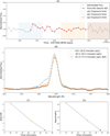 |
Fig. 1 LAMOST time-series spectra and TESS light curve during the stellar flare. Panel A: TESS normalised flux light curve of the flare. The blue shaded interval marks the first LAMOST exposure (sp1), the light orange interval the second (sp2), and the light brown interval the third (sp3). Panel B: time-series Hα line profiles obtained with LAMOST, with the same color scheme as in Panel (A). Panel C: temporal evolution of the excess EW of the Hα line (∆Hα EW). Panel D: dynamic evolution of the Hα line asymmetry, quantified as the difference between the EW of the blue and red wings. |
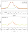 |
Fig. 2 Gaussian fits to the Hα line profiles during the flare. Panel A: double-Gaussian fit to the first Hα difference profile (normalised flare spectrum minus the normalised reference spectrum). Yellow dots denote the observed Hα line profile, the solid red line shows the total Gaussian fit, the dashed blue line marks the blueshifted component, and the dashed green line marks the redshifted component. The reduced χ2 value is indicated in the upper-left corner. The vertical dashed gray line marks the Hα rest wavelength in quiescence. Panel B: single-Gaussian fit to the second Hα difference profile. |
3.2 Mass estimation of the erupting prominence
The mass of the ejected stellar prominence is estimated by converting the excess emission detected in the blueshifted Hα wing into the number of hydrogen atoms required to produce that emission. The prominence-related enhancement is first quantified through an EW-like quantity,
 (3)
(3)
where Ablue and σblue denote the amplitude and Gaussian standard deviation of the blueshifted component identified in the first eruptive Hα spectrum. This quantity represents the wavelength-integrated excess emission associated with the outward moving plasma.
The luminosity of the prominence-related excess emission in the Hα line is obtained by multiplying Qprominence by the continuum luminosity per unit wavelength at the Hα wavelength,
 (4)
(4)
where the continuum luminosity at Hα is computed as
 (5)
(5)
Here, χ is the ratio of the local continuum flux adjacent to Hα to the stellar bolometric surface flux. For a stellar atmospheric model with T* = 3100 K, this fraction is χ = 2.736 × 10⁻⁵ (West et al. 2004; Fang et al. 2018). The parameters R*, T*, and σ denote the stellar radius, the stellar effective temperature, and the Stefan-Boltzmann constant, respectively. The Hα luminosity of the prominence is LHα,prominence = 3.61 × 1027 erg s−1.
Since no published non-local thermal-equilibrium (NLTE) population ratio is available for the Hα transition (Ntot/N3) in active M dwarfs, we converted the prominence-related Hα luminosity into an equivalent Hγ luminosity using a Balmer decrement appropriate for flare conditions on M-type stars. Following the observational and theoretical results of Katsova (1990), we adopted a flare-phase Balmer decrement of F(Hα)/F(Hγ) = 1.2. Since the Balmer decrement is defined as a ratio of line fluxes, the same relation applies to the corresponding line luminosities, yielding
 (6)
(6)
The prominence mass can then be estimated using the standard NLTE excitation formalism applied to the Hγ transition (e.g. Houdebine et al. 1990; Koller et al. 2021; Lu et al. 2022),
 (7)
(7)
Here hν5-2 and A5-2 are the photon energy and Einstein coefficient of the Hγ transition (j = 5 → i = 2), mH is the hydrogen mass, ηOD is an optical-depth correction factor, and Ntot/N5 denotes the NLTE-derived ratio between the total hydrogen population and the population in the upper level j = 5.
For the Hγ transition, we adopted Ntot/N5 = 2 × 10⁹, as derived from NLTE modelling of active M dwarfs (Houdebine et al. 1990; Koller et al. 2021). We further adopted an optical-depth correction factor ηOD = 2, corresponding to an escape probability of approximately 50% (Leitzinger et al. 2014), and use the Einstein coefficient A5-2 = 2.53 × 10⁶s−1 from the hydrogen transition-probability compilation of Wiese & Fuhr (2009). The inequality sign in Eq. (7) reflects that this expression provides a lower limit to the prominence mass. Only the hydrogen atoms contributing to the observed Hγ emission are directly accounted for, while additional material may remain optically thick, geometrically obscured, or insufficiently excited to emit efficiently in this transition. Moreover, the adopted NLTE population ratio and optical-depth correction factor are chosen conservatively, yielding the minimum mass required to reproduce the observed line luminosity. Using these Hγ transition parameters in Eq. (7), we obtain a lower-limit estimate for the prominence mass of approximately 1.74 × 10¹⁸g. Adopting the line-of-sight blueshifted bulk velocity of −84kms−1, the corresponding kinetic energy is Ekin ≥ 6.14 × 1031 erg.
The eruptive prominence mass derived above, Mprominence ≥ 1.74 × 10¹⁸ g, is orders of magnitude larger than the mass of typical solar eruptive prominences. For the Sun, the cool prominence cores embedded in CMEs generally contain ∼1014−1016 g of material (e.g. Vourlidas et al. 2010; Webb & Howard 2012). Thus, the stellar eruption studied here clearly represents a giant prominence ejection in terms of its expelled mass. Moreover, the erupting stellar prominence produces a pronounced excess emission component in the blue wing of the Hα line in our point-source spectrum. in contrast, Sun-as-a-star observations normally show only subtle Hα wing signatures during solar flares and filament eruptions, because disk integration strongly suppresses localised line asymmetries. Statistical studies of spatially resolved solar flares further demonstrate that Hα line asymmetries are usually dominated by red-wing enhancements associated with chromospheric condensation, whereas blue-wing emission is comparatively rare and typically associated with upward moving cool material such as surges or erupting filaments (e.g. Huang et al. 2014; Otsu et al. 2022; Liu et al. 2025). The combination of a clearly detectable blue-wing emission component together with the exceptionally large prominence mass therefore indicates that the event reported here is an unusually massive and energetic prominence ejection compared to solar eruptive prominences.
 |
Fig. 3 Flares detected on the M-dwarf LAMOST J063150.73+412942.2 from TESS observations in sectors 20 and 60. Panels A and B: normalised and de-trended TESS light curves, with flares marked by red asterisks. The normalised fluxes are shifted vertically for clarity. The pink arrow highlights the 60th flare, which is covered by the LAMOST spectroscopic observations. Panel C: Flare 26 in sector 20, with a peak flux of 1.100 and a flare energy of 2.67 × 1033 erg. Panel D: Flare 71, the most energetic flare in sector 60, with a peak flux of 1.897 and an energy of 8.04 × 1033 erg. |
3.3 Flare energy in the Hα band
The Hα flare energy refers to the radiative energy released in the Hα line, which generally represents only a small fraction of the bolometric flare energy, typically at the level of a few percent and in some cases up to ∼ 10% (e.g. Fuhrmeister et al. 2008; Kowalski et al. 2013). By subtracting a reference spectrum from the flare spectrum, we obtained the flare-induced change in Hα EW. The time-integrated EW during the flare can be written as
 (8)
(8)
The fraction of the total stellar radiation emitted in the Hα line, xHα, is determined from the stellar atmospheric model at Teff = 3100 K, giving xHα = 2.736 × 10⁻⁵ (West et al. 2004; Fang et al. 2018). The stellar bolometric luminosity is expressed as
 (9)
(9)
and the flare energy in the Hα band is then
 (10)
(10)
Substituting the parameters derived for the target star, we obtain an Hα flare energy of (7.7 ± 1.2) × 1030 erg.
4 Flare parameter analysis from TESS photometry
4.1 Flare detection and energy estimation
In this study, the stellar prominence eruption was observed simultaneously with TESS photometry and LAMOST time-resolved spectroscopy. The TESS data include two observing sectors (20 and 60), with sector 60 overlapping the LAMOST spectroscopic coverage. We first performed a global analysis of the flares detected in these two sectors. Similar to solar flares, stellar flares typically show a fast rise and a slower decay phase. Various approaches have been developed to detect such events from light curves. These methods can be broadly grouped into (1) subtraction of a background trend to remove rotational modulation, followed by identification of flare-like signals (e.g. Shibayama et al. 2013; Wu et al. 2015; Davenport 2016; Lu et al. 2019; Vasilyev et al. 2024), and (2) the application of machine-learning algorithms such as convolutional neural networks (e.g. Feinstein et al. 2020). We adopted the first approach, using normalisation and polynomial detrending of the TESS light curves, and then applied the altaipony package (Ilin et al. 2021; Ilin & Poppenhaeger 2022) to automatically identify flare candidates. Each candidate was visually inspected, yielding a final sample of 79 flares. These events are shown in Figs. 3A and 3B. The flare associated with the LAMOST spectroscopic prominence eruption corresponds to flare 60 in sector 60, indicated by the arrow in Fig. 3B. Two representative superflares are displayed in Figs. 3C and 3D.
Two methods are widely used to estimate stellar flare energies. The first assumes that the flare emission can be approximated by blackbody radiation, from which the total energy is derived (e.g., Shibayama et al. 2013; Davenport 2016). The second method, proposed by Wu et al. (2015), estimates the total energy by integrating the normalised light curve over time. This approach assumes that the flare temporal profile is similar across different wavelengths and computes the energy from the stellar luminosity, relative flare amplitude, and flare duration.
We adopted the blackbody radiation approach to estimate flare energies. The stellar luminosity in the observed passband is given by
 (11)
(11)
where R* is the stellar radius, T* is the effective temperature, and Rλ denotes the instrumental response function (TESS). The luminosity of a single flare is
 (12)
(12)
with Aflare(t) the flare area, assuming a constant temperature during the flare. The normalised flux enhancement is then
 (13)
(13)
We defined a scaling factor,
 (14)
(14)
which can be derived from the instrument response function and the stellar and flare effective temperatures (e.g. Petrucci et al. 2024; Su et al. 2025). By combining the above relations, the bolometric flare energy can be expressed as
 (15)
(15)
The flare temperature is typically assumed to be 10000 K to reproduce observed white-light flare spectra (e.g., Shibayama et al. 2013; Kowalski et al. 2013; Yang & Liu 2019). Uncertainties in flare temperature, instrumental calibration, and background subtraction typically result in energy errors of order ~60%.
Using the above formula, we calculated the energies of the 79 detected flares, which span a range of 8.19 × 1030 to 8.04 × 1033 erg. Flare 60 released an energy of 2.94 × 1031 erg, comparable to a solar X-class flare, and was accompanied by a giant stellar prominence eruption. This eruption is clearly manifested in the time-resolved point-source Hα spectra as a pronounced blue-wing enhancement, yielding a lower-limit prominence mass of 1.74 × 10¹⁸ g. From the LAMOST Hα spectra, we further estimate that the Hα energy of Flare 60 accounts for about 26(±4)% of its total radiative energy.
Our observations show that the bolometric energy released by the flare, Ebol ≃ 2.94 × 1031 erg, and the kinetic energy of the erupting prominence, Ekin ≃ 6.14 × 1031 erg, are comparable within an order of magnitude. This indicates a near equipartition between the radiative energy of the flare and the kinetic energy of the associated eruption. Such an energy partition is commonly observed in solar eruptive events. Comprehensive studies of large solar flares and their associated CMEs have shown that the total radiated flare energy and the CME kinetic energy are often of the same order (e.g. Emslie et al. 2012). Similar behaviour has also been reported for solar analogues, where simultaneous observations of superflares and filament eruptions on young Sunlike stars reveal eruption kinetic energies comparable to the flare radiative output (e.g. Namekata et al. 2021, 2024).
In contrast, this type of energy equipartition appears to be uncommon among M dwarfs. Previous observational and statistical studies indicate that, in red dwarfs, the kinetic energy of eruptions or CME-like events is typically much smaller than the corresponding flare energy (e.g. Moschou et al. 2019). Most eruptive flares on M dwarfs therefore fall into a regime in which radiative losses dominate the energy budget, and only a small fraction of the released magnetic energy is converted into large-scale mass ejection. Against this background, the event reported here represents a rare example of near equipartition between flare radiative energy and eruption kinetic energy on an M dwarf. In terms of energy partitioning, this behaviour more closely resembles that observed in solar and solar-type eruptive events, while deviating from the typical pattern inferred for active red dwarfs. This finding provides an important observational constraint on the diversity of energy release and transport processes in stellar magnetic eruptions and suggests that, under certain conditions, M dwarfs host eruptive events with energy coupling efficiencies comparable to those of the Sun and its analogues.
4.2 Analysis of the flare frequency distribution
The flare frequency distribution (FFD) is commonly described by a power-law form,
 (16)
(16)
where E is the flare energy and α the power-law index. Studies of solar flares indicate typical values of −1.5 ≲ α ≲ −1.8, with the exact slope depending on the observed wavelength and energy range (Crosby et al. 1993; Shimizu 1995; Aschwanden et al. 2000). Investigations of superflares on solar-type stars with Kepler have revealed similar distributions, with indices of α ≈ −1.8 (Shibayama et al. 2013; Maehara et al. 2015). More recent large-sample stellar flare surveys further confirm that the FFD slopes generally fall in the range −2.5 ≲ α ≲ −1.7, consistent with magnetic reconnection as a universal energy-release mechanism.
From the 79 flares detected in the TESS light curves, we find that their FFD follows a power-law distribution with an index of α = −1.52. This indicates that higher-energy flares occur less frequently and that a quantitative scaling relation exists between energy and frequency (Crosby et al. 1993; Shibayama et al. 2013; Maehara et al. 2015). Figure 4 shows the histogram of the flare occurrence rate as a function of energy, where we highlight Flare 60, which was simultaneously observed with LAMOST and TESS. Its location in the upper-left of the distribution illustrates that such low-energy flares are frequent, with an occurrence rate of about 290 events per year on this star. The derived slope is close to the solar values (−1.5 ≲ α ≲ −1.8; Crosby et al. 1993; Shimizu 1995; Aschwanden et al. 2000), suggesting that the statistical properties of magnetic energy release in this active M dwarf are similar to those on the Sun. However, although solar X-class flares can reach comparable energies, no evidence has yet been found for solar events accompanied by such large-scale prominence eruptions (e.g. Schrijver et al. 2012; Aulanier et al. 2013).
5 Summary
We present a joint analysis of TESS photometry and LAMOST medium-resolution spectroscopy for the active M dwarf LAMOST J063150.73+412942.2. From two TESS sectors, we identify 79 flares with bolometric energies in the range 8.19 × 1030−8.04 × 1033 erg. Their frequency distribution follows a power law with an index of α = −1.52, in good agreement with previous solar and stellar flare studies, indicating that the statistical properties of magnetic energy release on this star are similar to those observed in the solar atmosphere. In particular, Flare 60, a relatively low-energy event, has an estimated occurrence rate of ∼290 events per year, reflecting the high level of persistent magnetic activity on this M dwarf.
The simultaneous TESS-LAMOST observations of Flare 60 provide valuable constraints on flare-associated plasma motions. The temporal Hα line profiles exhibit clear blue-wing enhancements that are inconsistent with pure chromospheric evaporation and instead point to a stellar prominence eruption. Gaussian fits to the excess emission yield a maximum line-of-sight projected blueshifted velocity of −242 kms−1. From the integrated blue-wing enhancement, we derive a lower-limit prominence mass of 1.74 × 10¹⁸ g and a corresponding kinetic energy of 6.14 × 1031 erg. The associated white-light flare has a bolometric energy of 2.94 × 1031 erg, which is comparable to that of a solar X-class flare, implying a near equipartition between the flare radiative energy and the kinetic energy of the erupting prominence.
Although only a single spectroscopically confirmed prominence eruption was captured during the six available LAMOST epochs, the event constitutes a high-quality and unambiguous detection obtained under strictly simultaneous photometric and spectroscopic coverage. Such coordinated observations remain rare in M-dwarf time-domain studies, and even an individual well-observed event provides important diagnostic constraints on flare-driven plasma dynamics. The limited temporal coverage of the current spectroscopic data precludes a robust assessment of the intrinsic occurrence rate of such eruptions, leaving open the question of whether this event represents a genuinely rare phenomenon or reflects observational incompleteness.
The near equipartition between the flare radiative energy and eruption kinetic energy inferred for this event is uncommon among M dwarfs, for which eruptive events are typically found to carry significantly less energy than their associated flares (e.g. Moschou et al. 2019). In this respect, the event reported here exhibits an energy partition more reminiscent of solar and solar-type eruptive events (e.g. Emslie et al. 2012; Namekata et al. 2021, 2024). Its detection therefore highlights the diversity of energy release and transport processes in magnetically active low-mass stars and provides a valuable observational benchmark for testing models of stellar magnetic reconnection and mass ejection. If such events occur more frequently than currently inferred, they may have important implications for the space-weather environments of close-in exoplanets. Continued long-term photometric monitoring, combined with high-cadence, multi-epoch, and multi-wavelength spectroscopy, will be essential to establishing the frequency and physical diversity of these eruptive phenomena.
 |
Fig. 4 FFD of TIC 144282456. The horizontal axis shows the flare energy and the vertical axis the flare frequency. The blue circles connected by a step-like line represent the cumulative distribution of the 79 detected flares, with error bars indicating statistical uncertainties. The purple pentagram marks the special case of Flare 60, the flare accompanied by a stellar prominence eruption. The dashed red line shows the best-fit power-law relation (y = 1.68 × 10¹⁸ x−1.52), where y denotes the flare frequency and x the flare energy. |
Acknowledgements
This work is supported by the National Natural Science Foundation of China (NSFC) under grants 12473055, 12250006, and by the Guizhou University Natural Science Special Research Fund (Special Post) under project number 202358. It is further supported by the Guizhou Provincial Science and Technology Projects (grant No. QianKeHe-JiChu-MS[2025]695). The Guoshoujing Telescope (the Large Sky Area Multi-Object Fiber Spectroscopic Telescope, LAMOST) is a National Major Scientific Project built by the Chinese Academy of Sciences. Funding for the LAMOST project has been provided by the National Development and Reform Commission, and it is operated and managed by the National Astronomical Observatories, Chinese Academy of Sciences. We also acknowledge the use of data from TESS, obtained from the MAST archive at the Space Telescope Science Institute (STScI). Funding for the TESS mission has been provided by the NASA Explorer Program. STScI is operated by the Association of Universities for Research in Astronomy, Inc., under NASA contract NAS 5-26555. This research made use of the Python programming language and the scientific packages NumPy, SciPy, Astropy, and Matplotlib.
References
- Aarnio, A. N., Matt, S. P., & Stassun, K. G. 2012, ApJ, 760, 9 [NASA ADS] [CrossRef] [Google Scholar]
- Airapetian, V. S., Danchi, W. C., Dong, C. F., et al. 2018, arXiv e-prints [arXiv:1801.07333] [Google Scholar]
- Antolin, P., & Rouppe van der Voort, L. 2012, ApJ, 745, 152 [Google Scholar]
- Argiroffi, C., Reale, F., Drake, J. J., et al. 2019, Nat. Astron., 3, 742 [NASA ADS] [CrossRef] [Google Scholar]
- Aschwanden, M. J., Tarbell, T. D., Nightingale, R. W., et al. 2000, ApJ, 535, 1047 [Google Scholar]
- Aulanier, G., Démoulin, P., Schrijver, C. J., et al. 2013, A&A, 549, A66 [NASA ADS] [CrossRef] [EDP Sciences] [Google Scholar]
- Benz, A. O., & Güdel, M. 2010, ARA&A, 48, 241 [Google Scholar]
- Callingham, J. R., Tasse, C., Keers, R., et al. 2025, Nature, 647, 603 [Google Scholar]
- Chen, P. F. 2011, Liv. Rev. Sol. Phys., 8, 1 [Google Scholar]
- Chen, H., Tian, H., Li, L., et al. 2022, A&A, 659, A107 [NASA ADS] [CrossRef] [EDP Sciences] [Google Scholar]
- Chen, Y.-B., Lu, H.-P., Tian, H., et al. 2025, ApJ, 987, L22 [Google Scholar]
- Cliver, E. W., Schrijver, C. J., Shibata, K., & Usoskin, I. G. 2022, Liv. Rev. Sol. Phys., 19, 2 [NASA ADS] [CrossRef] [Google Scholar]
- Crosby, N. B., Aschwanden, M. J., & Dennis, B. R. 1993, Sol. Phys., 143, 275 [NASA ADS] [CrossRef] [Google Scholar]
- Crosley, M. K., & Osten, R. A. 2018, ApJ, 862, 113 [NASA ADS] [CrossRef] [Google Scholar]
- Crosley, M. K., Osten, R. A., Broderick, J. W., et al. 2016, ApJ, 830, 24 [NASA ADS] [CrossRef] [Google Scholar]
- Cui, X.-Q., Zhao, Y.-H., Chu, Y.-Q., et al. 2012, Res. Astron. Astrophys., 12, 1197 [Google Scholar]
- Davenport, J. R. A. 2016, ApJ, 829, 23 [Google Scholar]
- De Wilde, M., Pietrow, A. G. M., Druett, M. K., et al. 2025, A&A, 700, A275 [NASA ADS] [CrossRef] [EDP Sciences] [Google Scholar]
- Deng, L.-C., Newberg, H. J., Liu, C., et al. 2012, Res. Astron. Astrophys., 12, 735 [Google Scholar]
- Emslie, A. G., Dennis, B. R., Shih, A. Y., et al. 2012, ApJ, 759, 71 [Google Scholar]
- Fang, X.-S., Zhao, G., Zhao, J.-K., & Bharat Kumar, Y. 2018, MNRAS, 476, 908 [NASA ADS] [CrossRef] [Google Scholar]
- Feinstein, A. D., Montet, B. T., Ansdell, M., et al. 2020, AJ, 160, 219 [Google Scholar]
- Fuhrmeister, B., Liefke, C., Schmitt, J. H. M. M., & Reiners, A. 2008, A&A, 487, 293 [NASA ADS] [CrossRef] [EDP Sciences] [Google Scholar]
- Gopalswamy, N., Yashiro, S., Liu, Y., et al. 2005, J. Geophys. Res. (Space Phys.), 110, A09S15 [Google Scholar]
- Hardegree-Ullman, K. K., Apai, D., Bergsten, G. J., Pascucci, I., & López Morales, M. 2023, AJ, 165, 267 [NASA ADS] [CrossRef] [Google Scholar]
- Harrison, R. A. 1996, Sol. Phys., 166, 441 [NASA ADS] [CrossRef] [Google Scholar]
- Hawley, S. L., Covey, K. R., Knapp, G. R., et al. 2002, AJ, 123, 3409 [NASA ADS] [CrossRef] [Google Scholar]
- Houdebine, E. R., Foing, B. H., & Rodono, M. 1990, A&A, 238, 249 [NASA ADS] [Google Scholar]
- Howard, W. S., Corbett, H., Law, N. M., et al. 2019, ApJ, 881, 9 [NASA ADS] [CrossRef] [Google Scholar]
- Huang, Z., Madjarska, M. S., Koleva, K., et al. 2014, A&A, 566, A148 [NASA ADS] [CrossRef] [EDP Sciences] [Google Scholar]
- Ilin, E., & Poppenhaeger, K. 2022, MNRAS, 513, 4579 [NASA ADS] [CrossRef] [Google Scholar]
- Ilin, E., Schmidt, S. J., Poppenhäger, K., et al. 2021, A&A, 645, A42 [NASA ADS] [CrossRef] [EDP Sciences] [Google Scholar]
- Inoue, S., Iwakiri, W. B., Enoto, T., et al. 2024, ApJ, 969, L12 [Google Scholar]
- Katsova, M. M. 1990, Soviet Ast., 34, 614 [Google Scholar]
- Khodachenko, M. L., Ribas, I., Lammer, H., et al. 2007, Astrobiology, 7, 167 [CrossRef] [Google Scholar]
- Koller, F., Leitzinger, M., Temmer, M., et al. 2021, A&A, 646, A34 [NASA ADS] [CrossRef] [EDP Sciences] [Google Scholar]
- Konijn, D. C., Vedantham, H. K., Tasse, C., et al. 2025, A&A, 703, A198 [NASA ADS] [CrossRef] [EDP Sciences] [Google Scholar]
- Kowalski, A. F., Hawley, S. L., Wisniewski, J. P., et al. 2013, ApJS, 207, 15 [NASA ADS] [CrossRef] [Google Scholar]
- Lammer, H., Lichtenegger, H. I. M., Kulikov, Y. N., et al. 2007, Astrobiology, 7, 185 [NASA ADS] [CrossRef] [Google Scholar]
- Leitzinger, M., & Odert, P. 2022, Serb. Astron. J., 205, 1 [NASA ADS] [CrossRef] [Google Scholar]
- Leitzinger, M., Odert, P., Greimel, R., et al. 2014, MNRAS, 443, 898 [NASA ADS] [CrossRef] [Google Scholar]
- Lin, J., Raymond, J. C., & van Ballegooijen, A. A. 2004, ApJ, 602, 422 [NASA ADS] [CrossRef] [Google Scholar]
- Li, Y., Ding, M. D., Qiu, J., & Cheng, J. X. 2015, ApJ, 811, 7 [NASA ADS] [CrossRef] [Google Scholar]
- Li, Y., Ding, M. D., Hong, J., Li, H., & Gan, W. Q. 2019, ApJ, 879, 30 [NASA ADS] [CrossRef] [Google Scholar]
- Linsky, J. 2019, Host Stars and their Effects on Exoplanet Atmospheres, 955 (Switzerland AG: Springer Nature) [Google Scholar]
- Liu, N., Fu, J.-N., Zong, W., et al. 2019, Res. Astron. Astrophys., 19, 075 [CrossRef] [Google Scholar]
- Liu, C., Fu, J., Shi, J., et al. 2020, arXiv e-prints [arXiv:2005.07210] [Google Scholar]
- Liu, X., Hou, Y., Li, Y., et al. 2025, ApJ, 993, 126 [Google Scholar]
- Lu, H.-p., Zhang, L.-y., Shi, J., et al. 2019, ApJS, 243, 28 [NASA ADS] [CrossRef] [Google Scholar]
- Lu, H.-p., Tian, H., Zhang, L.-y., et al. 2022, A&A, 663, A140 [NASA ADS] [CrossRef] [EDP Sciences] [Google Scholar]
- Lu, H.-p., Tian, H., Chen, H.-c., et al. 2023, ApJ, 953, 68 [NASA ADS] [CrossRef] [Google Scholar]
- Lu, H.-P., Tian, H., Zhang, L.-Y., et al. 2025, ApJ, 978, L32 [NASA ADS] [CrossRef] [Google Scholar]
- Luo, A. L., Zhao, Y.-H., Zhao, G., et al. 2015, Res. Astron. Astrophys., 15, 1095 [Google Scholar]
- Maehara, H., Shibayama, T., Notsu, Y., et al. 2015, Earth Planets Space, 67, 59 [NASA ADS] [CrossRef] [Google Scholar]
- Maehara, H., Notsu, Y., Namekata, K., et al. 2021, PASJ, 73, 44 [NASA ADS] [CrossRef] [Google Scholar]
- Mason, J. P., Woods, T. N., Caspi, A., Thompson, B. J., & Hock, R. A. 2014, ApJ, 789, 61 [NASA ADS] [CrossRef] [Google Scholar]
- Milligan, R. O., & Dennis, B. R. 2009, ApJ, 699, 968 [NASA ADS] [CrossRef] [Google Scholar]
- Milligan, R. O., Gallagher, P. T., Mathioudakis, M., & Keenan, F. P. 2006, ApJ, 642, L169 [NASA ADS] [CrossRef] [Google Scholar]
- Mohan, A., Mondal, S., Wedemeyer, S., & Gopalswamy, N. 2024, A&A, 686, A51 [NASA ADS] [CrossRef] [EDP Sciences] [Google Scholar]
- Moschou, S.-P., Drake, J. J., Cohen, O., et al. 2019, ApJ, 877, 105 [NASA ADS] [CrossRef] [Google Scholar]
- Muheki, P., Guenther, E. W., Mutabazi, T., & Jurua, E. 2020, MNRAS, 499, 5047 [NASA ADS] [CrossRef] [Google Scholar]
- Namekata, K., Maehara, H., Honda, S., et al. 2021, Nat. Astron., 6, 241 [Google Scholar]
- Namekata, K., Airapetian, V. S., Petit, P., et al. 2024, ApJ, 961, 23 [Google Scholar]
- Notsu, Y., Kowalski, A. F., Maehara, H., et al. 2024, ApJ, 961, 189 [NASA ADS] [CrossRef] [Google Scholar]
- Otsu, T., & Asai, A. 2024, ApJ, 964, 75 [NASA ADS] [CrossRef] [Google Scholar]
- Otsu, T., Asai, A., Ichimoto, K., Ishii, T. T., & Namekata, K. 2022, ApJ, 939, 98 [NASA ADS] [CrossRef] [Google Scholar]
- Pecaut, M. J., & Mamajek, E. E. 2013, ApJS, 208, 9 [Google Scholar]
- Peter, H. 2001, A&A, 374, 1108 [NASA ADS] [CrossRef] [EDP Sciences] [Google Scholar]
- Petrucci, R. P., Gómez Maqueo Chew, Y., Jofré, E., Segura, A., & Ferrero, L. V. 2024, MNRAS, 527, 8290 [Google Scholar]
- Ricker, G. R., Winn, J. N., Vanderspek, R., et al. 2015, J. Astron. Telesc. Instrum. Syst., 1, 014003 [Google Scholar]
- Schrijver, C. J., Beer, J., Baltensperger, U., et al. 2012, J. Geophys. Res. (Space Phys.), 117, A08103 [Google Scholar]
- Segura, A., Walkowicz, L. M., Meadows, V., Kasting, J., & Hawley, S. 2010, Astrobiology, 10, 751 [Google Scholar]
- Shibayama, T., Maehara, H., Notsu, S., et al. 2013, ApJS, 209, 5 [Google Scholar]
- Shimizu, T. 1995, PASJ, 47, 251 [NASA ADS] [Google Scholar]
- Su, T., Zhang, L.-y., Misra, P., et al. 2025, ApJS, 276, 44 [Google Scholar]
- Temmer, M. 2021, Liv. Rev. Sol. Phys., 18, 4 [NASA ADS] [CrossRef] [Google Scholar]
- Tian, H., McIntosh, S. W., De Pontieu, B., et al. 2011, ApJ, 738, 18 [NASA ADS] [CrossRef] [Google Scholar]
- Tian, H., Young, P. R., Reeves, K. K., et al. 2015, ApJ, 811, 139 [NASA ADS] [CrossRef] [Google Scholar]
- Tian, H., Xu, Y., Chen, H., et al. 2023, Sci. Sinica Technol., 53, 2021 [Google Scholar]
- Vasilyev, V., Reinhold, T., Shapiro, A. I., et al. 2024, Science, 386, 1301 [Google Scholar]
- Veronig, A. M., Odert, P., Leitzinger, M., et al. 2021, Nat. Astron., 5, 697 [NASA ADS] [CrossRef] [Google Scholar]
- Veronig, A. M., Dissauer, K., Kliem, B., et al. 2025, Liv. Rev. Sol. Phys., 22, 2 [Google Scholar]
- Vida, K., Leitzinger, M., Kriskovics, L., et al. 2019, A&A, 623, A49 [NASA ADS] [CrossRef] [EDP Sciences] [Google Scholar]
- Vida, K., Kovári, Z., Leitzinger, M., et al. 2024, Universe, 10, 313 [Google Scholar]
- Vourlidas, A., Howard, R. A., Esfandiari, E., et al. 2010, ApJ, 722, 1522 [NASA ADS] [CrossRef] [Google Scholar]
- Wang, R., Luo, A. L., Chen, J. J., et al. 2019, ApJS, 244, 27 [NASA ADS] [CrossRef] [Google Scholar]
- Webb, D. F., & Howard, T. A. 2012, Liv. Rev. Sol. Phys., 9, 3 [Google Scholar]
- West, A. A., Hawley, S. L., Walkowicz, L. M., et al. 2004, AJ, 128, 426 [NASA ADS] [CrossRef] [Google Scholar]
- Wiese, W. L., & Fuhr, J. R. 2009, J. Phys. Chem. Ref. Data, 38, 565 [Google Scholar]
- Wu, C.-J., Ip, W.-H., & Huang, L.-C. 2015, ApJ, 798, 92 [Google Scholar]
- Xu, Y., Tian, H., Hou, Z., et al. 2022, ApJ, 931, 76 [NASA ADS] [CrossRef] [Google Scholar]
- Xu, Y., Alvarado-Gómez, J. D., Tian, H., et al. 2024, ApJ, 971, 153 [Google Scholar]
- Yang, H., & Liu, J. 2019, ApJS, 241, 29 [NASA ADS] [CrossRef] [Google Scholar]
- Yelle, R., Lammer, H., & Ip, W.-H. 2008, Space Sci. Rev., 139, 437 [Google Scholar]
- Yu, K., Li, Y., Ding, M. D., et al. 2020, ApJ, 896, 154 [Google Scholar]
- Yiu, T. W. H., Vedantham, H. K., Callingham, J. R., & Günther, M. N. 2024, A&A, 684, A3 [NASA ADS] [CrossRef] [EDP Sciences] [Google Scholar]
- Zhang, B., Li, J., Yang, F., et al. 2021, ApJS, 256, 14 [NASA ADS] [CrossRef] [Google Scholar]
- Zhao, G., Zhao, Y.-H., Chu, Y.-Q., Jing, Y.-P., & Deng, L.-C. 2012, Res. Astron. Astrophys., 12, 723 [NASA ADS] [CrossRef] [Google Scholar]
All Figures
|
Fig. 1 LAMOST time-series spectra and TESS light curve during the stellar flare. Panel A: TESS normalised flux light curve of the flare. The blue shaded interval marks the first LAMOST exposure (sp1), the light orange interval the second (sp2), and the light brown interval the third (sp3). Panel B: time-series Hα line profiles obtained with LAMOST, with the same color scheme as in Panel (A). Panel C: temporal evolution of the excess EW of the Hα line (∆Hα EW). Panel D: dynamic evolution of the Hα line asymmetry, quantified as the difference between the EW of the blue and red wings. |
| In the text | |
|
Fig. 2 Gaussian fits to the Hα line profiles during the flare. Panel A: double-Gaussian fit to the first Hα difference profile (normalised flare spectrum minus the normalised reference spectrum). Yellow dots denote the observed Hα line profile, the solid red line shows the total Gaussian fit, the dashed blue line marks the blueshifted component, and the dashed green line marks the redshifted component. The reduced χ2 value is indicated in the upper-left corner. The vertical dashed gray line marks the Hα rest wavelength in quiescence. Panel B: single-Gaussian fit to the second Hα difference profile. |
| In the text | |
|
Fig. 3 Flares detected on the M-dwarf LAMOST J063150.73+412942.2 from TESS observations in sectors 20 and 60. Panels A and B: normalised and de-trended TESS light curves, with flares marked by red asterisks. The normalised fluxes are shifted vertically for clarity. The pink arrow highlights the 60th flare, which is covered by the LAMOST spectroscopic observations. Panel C: Flare 26 in sector 20, with a peak flux of 1.100 and a flare energy of 2.67 × 1033 erg. Panel D: Flare 71, the most energetic flare in sector 60, with a peak flux of 1.897 and an energy of 8.04 × 1033 erg. |
| In the text | |
|
Fig. 4 FFD of TIC 144282456. The horizontal axis shows the flare energy and the vertical axis the flare frequency. The blue circles connected by a step-like line represent the cumulative distribution of the 79 detected flares, with error bars indicating statistical uncertainties. The purple pentagram marks the special case of Flare 60, the flare accompanied by a stellar prominence eruption. The dashed red line shows the best-fit power-law relation (y = 1.68 × 10¹⁸ x−1.52), where y denotes the flare frequency and x the flare energy. |
| In the text | |
Current usage metrics show cumulative count of Article Views (full-text article views including HTML views, PDF and ePub downloads, according to the available data) and Abstracts Views on Vision4Press platform.
Data correspond to usage on the plateform after 2015. The current usage metrics is available 48-96 hours after online publication and is updated daily on week days.
Initial download of the metrics may take a while.