| Issue |
A&A
Volume 690, October 2024
|
|
|---|---|---|
| Article Number | A305 | |
| Number of page(s) | 7 | |
| Section | Stellar atmospheres | |
| DOI | https://doi.org/10.1051/0004-6361/202450931 | |
| Published online | 16 October 2024 | |
Flare-related plasma motions in the outer atmosphere of the RS CVn-type star II Peg
1
Yunnan Observatories, Chinese Academy of Sciences,
Kunming
650216,
China
2
Key Laboratory for the Structure and Evolution of Celestial Objects, Chinese Academy of Sciences,
Kunming
650216,
China
3
International Centre of Supernovae, Yunnan Key Laboratory,
Kunming
650216,
China
4
School of Astronomy and Space Science, University of Chinese Academy of Sciences,
Beijing
101408,
China
★ Corresponding author; This email address is being protected from spambots. You need JavaScript enabled to view it.
; This email address is being protected from spambots. You need JavaScript enabled to view it.
Received:
31
May
2024
Accepted:
11
September
2024
Abstract
Analogous to solar flares, stellar flares are dramatic explosions in the atmosphere, which may be accompanied by prominence eruptions, coronal mass ejections (CMEs), and other forms of plasma motion. Based on time-resolved spectroscopic observations of the RS CVn-type star II Peg, we aim to search for the potential plasma motions associated with flares. In these observations, we detected part of the gradual decay phase of an optical flare, for which we find a lower limit on the energy of the Hα line of 6.03 × 1033 erg. Converting this Hα energy, we find a bolometric white-light energy of 3.10 × 1035 erg. Moreover, a secondary peak is also observed. After removing a quiescence reference, the Hα residual shows an asymmetric behavior, including both a blueshifted and a redshifted emission component. The former component has a bulk velocity of about −180 km s−1 and extends its velocity to more than −350 km s−1. This phenomenon is likely caused by a prominence eruption event or a chromospheric evaporation process. The latter emission component has a bulk velocity of 130–70 km s−1 and extends its velocity to nearly 400 km s−1. We attribute the redshifted emission component to one or a combination of several possible scenarios: flare-driven coronal rain, chromospheric condensation, backward-directed prominence eruption close to the stellar limb, or falling material in a prominence eruption. The minimum masses of the moving plasmas resulting in the blueshifted and redshifted emission components are estimated to be 0.56 × 10²⁰ g and 1.74 × 10²⁰ g, respectively.
Key words: Sun: filaments, prominences / stars: activity / stars: coronae / stars: flare / stars: magnetic field
© The Authors 2024
 Open Access article, published by EDP Sciences, under the terms of the Creative Commons Attribution License (https://creativecommons.org/licenses/by/4.0), which permits unrestricted use, distribution, and reproduction in any medium, provided the original work is properly cited.
This article is published in open access under the Subscribe to Open model. This email address is being protected from spambots. You need JavaScript enabled to view it. to support open access publication.
1 Introduction
Solar flares are dramatic explosion events in the outer atmosphere of the Sun. They can be accompanied by prominence eruptions and coronal mass ejections (CMEs), which have significant influences on space weather (e.g., Forbes 2000; Koleva et al. 2021). Although flares and even superflares are frequently observed on late-type stars (e.g., Maehara et al. 2012; Tu et al. 2020, 2021; Yang et al. 2023), particularly in the surveys of the Kepler space telescope and the Transiting Exoplanet Survey Satellite (TESS), reported stellar prominence eruption and CME events are rare.
In recent years, stellar CMEs have attracted much attention for their significant impacts on mass and angular momentum loss in the course of stellar evolution (e.g., Aarnio et al. 2012; Osten & Wolk 2015) and the potential habitability of the surrounding exoplanets (e.g., Airapetian et al. 2016; Cherenkov et al. 2017; Hazra et al. 2022; Cohen et al. 2022). Because direct imaging of stellar CMEs – as performed on the Sun – is impossible with current instrumentation, their detection is mainly based on other observational signatures known from studies of solar CMEs. Detailed reviews of the different methodologies used to attempt the detection of stellar CMEs can be found in Leitzinger & Odert (2022) and Tian et al. (2023). In the optical wavelength regions, stellar CME candidates can be detected using the features of Doppler-shifted emission and absorption in the wings of sensitive chromospheric lines, especially the Balmer lines (e.g., Houdebine et al. 1990; Vida et al. 2019; Leitzinger et al. 2020; Koller et al. 2021; Namekata et al. 2021; Lu et al. 2022; Wu et al. 2022; Inoue et al. 2023). If the CME lies directly on the line of sight to the observer, it may produce an absorption signature (see Namekata et al. 2021). In addition to obtaining spectroscopic observations of individual stars, research has also been conducted to detect possible stellar CMEs by investigating a large number of stars based on archival data (Fuhrmeister et al. 2018; Vida et al. 2019; Leitzinger et al. 2020; Koller et al. 2021; Lu et al. 2022).
It is widely acknowledged that the possible CME signatures identified in the optical spectral line profiles mostly correspond to eruptive prominences, which are believed to form the CME cores in the frequently observed three-part structure of solar CMEs (Forbes 2000). With the exception of prominence eruptions and CMEs, the Doppler-shifted emission and absorption signatures observed in the chromospheric line profiles can also be attributed to other forms of plasma motion during the flares, including chromospheric evaporation (e.g., Li & Ding 2011; Tei et al. 2018; Honda et al. 2018), chromospheric condensation (e.g., Ichimoto & Kurokawa 1984; Tei et al. 2018; Vida et al. 2019), and coronal rain (e.g., Antolin et al. 2012; Lacatus et al. 2017; Li et al. 2021).
In this study, we present the results of time-resolved highresolution spectroscopic observations of one of the most active RS CVn-type stars, II Pegasi (II Peg). It is notable that the Hα line profile shows flare-related asymmetric behavior during our observation, which implies the existence of moving plasmas in the outer atmosphere of II Peg during the flare. This observation provides valuable insights that will contribute to the future detection and identification of stellar prominence eruptions and CMEs.
II Peg (= HD 224085) is a single-lined spectroscopic binary system, consisting of a K2 IV primary star and an unseen secondary companion with a period of about 6.7 days (Berdyugina et al. 1998). More detailed information regarding the physical parameters of II Peg can be found in our previous paper (Cao & Gu 2024). The K2 IV primary star shows remarkable photometric starspot activity (e.g., Vogt 1981; Berdyugina & Tuominen 1998; Rodonò et al. 2000; Lindborg et al. 2013), intense Ca II H&K and Hα line emission (e.g., Vogt 1981; Huenemoerder & Ramsey 1987; Montes et al. 1997; Berdyugina et al. 1999; Frasca et al. 2008), and strong UV and X-ray radiation (e.g., Byrne et al. 1989; Ercolano et al. 2008). Moreover, II Peg is a high-rate flaring star, showing flares several times in the optical, UV, and X-ray wavelength bands (e.g., Rodono et al. 1987; Doyle et al. 1991; Berdyugina et al. 1999; Frasca et al. 2008; Ercolano et al. 2008; Siwak et al. 2010; Tsuboi et al. 2016; Cao & Gu 2024). Therefore, based on the close association between solar CMEs and flares, II Peg is expected to produce frequent CME events. Recently, we detected a highly redshifted emission signature in the high-resolution Hα spectra during a stronger flare on II Peg (Cao & Gu 2024). The redshifted emission signature can be explained by a possible CME with backward propagation due to its fast Doppler-shift velocity or chromospheric condensation.
In Sec. 2, we provide details of our high-resolution spectroscopic observation and data reduction. Our spectral analysis is described in Sect. 3, especially for the Hα line. In Sect. 4, we provide a more detailed discussion of a particular optical flare event and the asymmetric Hα line profile. Finally, we conclude and summarize our findings in Sec. 5.
2 Spectroscopic observation and data reduction
Spectra of II Peg analyzed in the present work were obtained during the night of 2015 October 30. The observation was performed with the fiber-fed high-resolution spectrograph (HRS, Fan et al. 2016) installed on the 2.16m telescope at the Xinglong station of the National Astronomical Observatories, Chinese Academic of Sciences, China. HRS produces spectra with a resolving power of R = λ/Δλ ≃ 48 000 in a wavelength range of 3900–10 000 Å, using a 4096 × 4096 pixel CCD detector to record spectra.
During our observation, a total of ten spectra of II Peg were obtained over a six-hour period. The first eight spectra had an exposure time of 900 s, while the last two had an exposure time of 1800 s. The signal-to-noise ratio (S/N) at the continuum near the Hα line region was around 200. To clearly indicate the time variation of our observation, we set the observation time (the mid-exposure of observation) of the first spectrum to zero and then derived the observation time of the other spectra.
The data reduction was performed with the IRAF1 package, following the standard procedures (see the prescription in Cao & Gu 2024). Moreover, for our observation, there were heavy telluric water vapor lines in the activity line regions of interest, especially in the Hα and He I D3 line regions. We eliminated these using the spectrum of a brighter and rapidly rotating early-type star HR 8858 (spectral type: B5 V, υ sin i = 316 km s−1) as a telluric line template, with an interactive procedure in the IRAF package.
3 Spectral analysis
Figure 1 shows the Hα, Hβ, and He I D3 line profiles obtained during our observation, in which the radial velocity of all spectra are corrected so that they are aligned. From the figure, we can see that the Hα line shows an emission feature above the continuum level and has a significantly variable profile. In particular, the red wing gradually decreased from a strong enhancement to being almost flat. Moreover, the Hβ line profile is characterized by a deep absorption feature, but significant changes also found in its red wing, which is consistent with the behavior of the Hα line profile. Finally, it can be seen that the He I D3 line shows a weak emission feature in the first two spectra, and then the emission disappears in the next two spectra. From the fifth to the eighth spectrum, it is noteworthy that a stronger emission feature reappears in the He I D3 line, and then disappears in the last two spectra.
To analyze the variation of the Hα line profile shown in Fig. 2a, we subtracted the last spectrum from the first nine. This is reasonable because the red wing of the last Hα profile had become flat, and there was no emission feature in the corresponding He I D3 line region, which means that there is no special activity at that time. Therefore, the last Hα profile can be used as a quiescence reference of the flare. We then obtained the quiescence reference-subtracted Hα line profiles (hereafter referred to as Hα residuals) shown in Fig. 2b. With the Hα residual, we model the line profile using a Gaussian fitting method. It can be seen that the profile can be well fitted by a weaker blueshifted broad emission component, a nearly centred narrow emission component, and a stronger redshifted broad emission component. From the figure, it is obvious that the intensity of the blueshifted emission component is weaker than the redshifted emission component, and that the duration of the blueshifted component is shorter than the redshifted one. Due to low S/N, however, we were not able to carry out any further analysis of the Hβ line.
We measured the equivalent widths (EWs) of the total Hα residual, and the blueshifted, central, and redshifted emission components, as well as their bulk velocities. Furthermore, we plot the time evolution of these measured values in Fig. 3.
4 Results and discussion
4.1 Optical flare
Typically, solar and stellar flares can be observed across the entire electromagnetic spectrum from shorter X-rays to longer radio wavelengths (Schrijver & Zwaan 2000). In the optical spectral range, the He I D3 line is an important and commonly used indicator to capture the flare activity events in solar and stellar chromospheres. Due to its very high excitation potential, the He I D3 line shows emission features above the continuum when an optical flare happens (see Zirin 1988; Gu et al. 2002; Cao et al. 2019, 2023; Cao & Gu 2024). Moreover, the other chromospheric sensitivity lines, especially the Hα line, also show stronger emission and variable line profiles during the flares. Therefore, the appearing and disappearing features of the He I D3 line emission and the variation of the Hα line profile might indicate an evolved flare activity event during our observations. Due to the limited nature of our observations, we did not capture the entire flare evolution from the initial outburst to the end. From Fig. 3, it can be seen that the EW of the Hα residual shows a decreasing trend from the starting observation to 93 minutes, which is consistent with the disappearance of the He I D3 emission feature. Therefore, it is believed that we captured part of the gradual decay phase of an optical flare during our observation.
Moreover, from Fig. 3, it is noteworthy that the EW of the Hα residual gradually increases between 93 and 167 minutes, and then decreases after 167 minutes, which implies the occurrence of a secondary peak during the flare decay phase. We were able to confirm the secondary peak by capturing the reappearance of the He I D3 line emission feature at the corresponding phases (see Fig. 1 and the description in Sect. 3).
We computed the stellar continuum flux ![Mathematical equation: $\[F_{\mathrm{H}_\alpha}\]$](/articles/aa/full_html/2024/10/aa50931-24/aa50931-24-eq1.png) (in erg cm−2 s−1 Å−1) near the Hα line region as a function of the color index B − V (~1.031 for II Peg; Messina 2008) based on the empirical relationship:
(in erg cm−2 s−1 Å−1) near the Hα line region as a function of the color index B − V (~1.031 for II Peg; Messina 2008) based on the empirical relationship:
![Mathematical equation: $\[\begin{array}{r}\log F_{\mathrm{H} \alpha}=[7.538-1.081(B-V)] \pm 0.33 \\0.0 \leq B-V \leq 1.4\end{array}\]$](/articles/aa/full_html/2024/10/aa50931-24/aa50931-24-eq2.png) (1)
(1)
from Hall (1996), and then converted the EW of the Hα residual into an absolute surface flux FS (in erg cm−2 s−1). Based on the derived flux FS, we were able to calculate the luminosity ![Mathematical equation: $\[F_{\mathrm{H}_\alpha}\]$](/articles/aa/full_html/2024/10/aa50931-24/aa50931-24-eq3.png) (in erg s−1) using the stellar radius = 3.4 R⊙ (Berdyugina et al. 1998) of the K2 IV primary star of II Peg. Thus, we found the luminosity
(in erg s−1) using the stellar radius = 3.4 R⊙ (Berdyugina et al. 1998) of the K2 IV primary star of II Peg. Thus, we found the luminosity ![Mathematical equation: $\[F_{\mathrm{H}_\alpha}\]$](/articles/aa/full_html/2024/10/aa50931-24/aa50931-24-eq4.png) of the flare to vary from 1.36 × 1030 erg s−1 to 0.51 × 1030 erg s−1 during our observation. Finally, integrating the luminosity of each flaring spectrum over the exposure time and then adding them together, the energy released in the Hα line is estimated to be approximately 6.03 × 1033 erg, which is the lower limit of the flare energy. Moreover, according to the empirical relationship between the Hα (EHα) and bolometric white-light (EWL,bol) flare energy from Namekata et al. (2024):
of the flare to vary from 1.36 × 1030 erg s−1 to 0.51 × 1030 erg s−1 during our observation. Finally, integrating the luminosity of each flaring spectrum over the exposure time and then adding them together, the energy released in the Hα line is estimated to be approximately 6.03 × 1033 erg, which is the lower limit of the flare energy. Moreover, according to the empirical relationship between the Hα (EHα) and bolometric white-light (EWL,bol) flare energy from Namekata et al. (2024):
![Mathematical equation: $\[\frac{E_{W L, bol }}{10^{33} ~\mathrm{erg}}=10^{1.68 \pm 0.15}\left(\frac{E_{\mathrm{H} \alpha}}{10^{33} ~\mathrm{erg}}\right)^{1.04 \pm 0.07},\]$](/articles/aa/full_html/2024/10/aa50931-24/aa50931-24-eq5.png) (2)
(2)
the bolometric white-light flare radiation energy, EWL,bol, is calculated to be approximately 3.10 × 1035 erg, which is comparable to the energy of stellar superflares, which release energies of more than 1033 erg.
 |
Fig. 1 Time variation of the Hα, Hβ, and He I D3 line profiles of II Peg observed on 2015 Oct 30. The He I D3 line profiles are shifted on the y-axis for illustrative purposes. |
4.2 Interpretation of the Hα asymmetry
During our observation, the Hα residual shows asymmetry, including a blueshifted emission component and a redshifted emission one, which suggests the existence of moving plasmas in the atmosphere during the flare on II Peg. Moreover, as shown in Fig. 3a, an increasing trend is seen in the intensities of the blueshifted, central, and redshifted emission components during the secondary peak; this trend is particularly evident for the redshifted emission component. The observed increase in the central emission component may indicates a secondary flare occurring during the decay phase of the main flare. Additionally, the observed increase in the blueshifted and redshifted emission components may be indicative of a notable increase in the scale of the moving plasmas.
 |
Fig. 2 Time variation of the Hα spectrum. (a) The first nine Hα spectra (black solid lines) are compared with the last one. The red dashed line represents the last spectrum observed at phase 0.809. (b) The Hα residuals between the first nine spectra and the last spectrum are shown and fitted using Gaussian fitting (dashed lines). |
4.2.1 Blueshifted emission component
Based on the current knowledge of solar flares, the blueshifted emission component could be ascribed to upward plasma flow above the chromospheric evaporation flows or an erupting prominence moving toward the observer (e.g., Canfield et al. 1990; Li & Ding 2011; Tei et al. 2018; Honda et al. 2018; Otsu et al. 2022).
In the case examined here, the blueshifted emission component has a bulk velocity of nearly −180 km s−1 (see Fig. 3) and extends its velocity to more than −350 km s−1 on the blue side. The higher Doppler velocity is likely indicative of a prominence eruption, and part of the prominence material may have escaped from the star, developing into a CME, given the maximum velocity of the blueshifted emission component, which exceeds the escape velocity (~306 km s−1, see Cao & Gu 2024) at the surface of the K2 IV primary star of II Peg. Moreover, it is important to note that the velocity mentioned is only the projection component along the line of sight. Accordingly, if there were a larger angle between the eruption direction and the line of sight, the true eruption velocity would be significantly greater, thereby increasing the probability that the above interpretation is accurate.
Chromospheric evaporation usually occurs in the early phase of a solar flare and is caused by upward moving material driven by intense chromospheric heating, with typical velocities in the range of tens of kilometers per second (e.g., Kennedy et al. 2015; Fuhrmeister et al. 2018; Tei et al. 2018). For our situation, the velocity of the blueshifted emission component is greater than the typical upward velocity of solar chromospheric evaporation. Because the energy scale of the flare on II Peg greatly exceeds that of typical solar flares, the magnitude of the blueshifted phenomena may be very different between solar flares and flares on stars. Therefore, it is also possible that the blueshifted emission component is caused by chromospheric evaporation. Moreover, the increasing intensity of the blueshifted emission component during the secondary peak may suggest that chromospheric evaporation becomes prominent, which is likely due to the additional heating of the chromosphere caused by the secondary flare.
4.2.2 Redshifted emission component
In contrast to the blueshifted emission component, the origin of the redshifted component is more complex. During our observation, the redshifted component has a bulk velocity of 130–70 km s−1 and extends its velocity to nearly 400 km s−1 on the red side (see Figs. 3b and 2b). According to our current knowledge of solar flares and the available literature for flares on other stars (e.g., Fuhrmeister et al. 2018; Koller et al. 2021; Wu et al. 2022; Cao & Gu 2024), there are several possible interpretations of the redshifted emission component, including flare-driven coronal rain, chromospheric condensation, a backward-directed prominence eruption, or falling material in a prominence eruption.
Coronal rain is a frequently observed phenomenon in the solar atmosphere. Flare-driven coronal rain usually forms as a result of the radiative cooling process of hot flaring plasma in post-flare loops and then falls down along post-flare loops to the surface under the effect of gravity. Thus, coronal rain often becomes more pronounced during the decay phase of flares and plays a fundamental role in the mass cycle between the corona and chromosphere (e.g., Li et al. 2021; Kohutova et al. 2019). The typical velocities of coronal rain range from 30 to 200 km s−1, with an average value of about 60–70 km s−1 (e.g., Antolin et al. 2012; Lacatus et al. 2017). The redshifted emission component seen in the observations presented here has the observational characteristics of coronal rain and the post-flare loops might become prominent during the secondary peak.
Chromospheric condensation is usually observed during the impulsive phases of solar flares and is caused by downward-moving material driven by the nonthermal electron beams of the flares. The typical downward mass velocity is approximately tens of kilometers per second, and sometimes even reaches or exceeds 100 km s−1 (Ichimoto & Kurokawa 1984; Tei et al. 2018). As opposed to our interpretation of the blueshifted emission component as chromospheric evaporation, the redshifted emission component could be attributed to chromospheric condensation, and the likelihood of this phenomenon is particularly elevated during the secondary peak, which is due to the occurrence of a secondary flare.
A backward-directed prominence eruption could also result in the redshifted emission component and a detectable backward-directed prominence eruption requires special spatial location (e.g., Moschou et al. 2019; Koller et al. 2021; Wu et al. 2022). In our previous paper (Cao & Gu 2024), we reported a possible backward-directed prominence eruption event, showing the redshifted emission component in the high-resolution spectra with a large bulk velocity of about 429 km s−1. The large velocity greatly exceeds the escape velocity of the K2 IV star of II Peg, which indicates that the prominence eruption can develop into a CME. In the present case, the redshifted emission component could also be attributed to a backward-directed prominence eruption near the stellar limb. On the one hand, similar to the blueshifted emission component, the velocity is only the component along the line of sight. When the prominence eruption occurs close to the stellar limb, the eruption velocity would be much greater than the measured Doppler velocity. Furthermore, the maximum velocity of the reshifted emission component extends beyond the escape velocity of II Peg. Therefore, it is possible that this prominence eruption could also develop into a CME.
Strong magnetic field on active stars may prevent prominence material from leaving the stellar surface (Drake et al. 2016; Alvarado-Gómez et al. 2018), thus falling material in a prominence eruption would also result in a redshifted emission component. Wu et al. (2022) depicted a similar scenario where the erupted prominence material may be confined by an overlying magnetic field, subsequently exhibiting downward material falling onto the stellar disk. This scenario could potentially account for the redshifted emission component in our observation. Moreover, the falling material would also result in flare heating and this would explain the occurrence of a secondary flare during the flare decay. For instance, Li & Ding (2017) reported a variety of flare brightenings associated with falling prominence material in the extreme-ultraviolet (EUV) passband on the Sun, including the two ribbon-like brightenings caused by the prominence material hitting the chromosphere when it falls back to the solar surface. These authors also reported brightenings resulting from the magnetic reconnection between the prominence magnetic structure and the surrounding magnetic field, and a thread-like brightening on top of the erupting magnetic field caused by an energy imbalance from a fast drop of radiative cooling due to plasma rarefaction. As shown in Fig. 3b, the velocity of the redshifted emission component we see appears to gradually slow down, which is probably because falling prominence material was influenced by the surrounding magnetic field and therefore slowed down by magnetic drag force (Li & Ding 2017). Thus, the magnetic reconnection between the prominence magnetic structure and the surrounding magnetic field may be the main mechanism triggering the occurrence of the secondary flare during our observation. Although the flare brightenings described by Li & Ding (2017) were observed in the EUV passband, it is possible that similar flare brightenings could also be found in the Hα line, because flares usually produce radiation across the entire electromagnetic spectrum. Finally, as stated by Wu et al. (2022), prior to the detection of the red asymmetry caused by falling material in a prominence eruption, there should be a short-lived blueshift ascribed to the ejecting prominence material at the flare onset. In our case, the entire life cycle of the flare was not captured by our observations. Therefore, we are not sure whether or not there was a blueshift at the flare onset. For our situation, if the blueshifted emission component is caused by the prominence eruption, we can assume it might be the continuation of the one that occurred at the flare onset and led to prominence material falling during our observation. However, the velocity of the blueshifted emission component is nearly stable and shows no decreasing trend (see Fig. 3b), probably because the prominence eruption is not a brief process and comprises an array of materials with different velocities.
Stellar flares are highly dramatic explosions that can be accompanied by prominence eruptions, CMEs, and other forms of plasma motion. As a result, the observed Hα features during the flare may represent a combination of the flare itself, a prominence eruption, a CME, and other plasma motions. Taking into consideration the evolutionary behavior of the redshifted emission component in the Hα residual of II Peg, it is possible that this phenomenon might also be caused by a combination of some of the aforementioned phenomena. For instance, in the scenarios of backward-directed prominence eruptions and falling material in prominence eruptions, the increasing scale of the redshifted emission component may be attributed to other forms of plasma motion, such as coronal rain or chromospheric condensation.
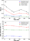 |
Fig. 3 Time evolution of the measurements for the total Hα residual and each fitted component during our observation. (a) EWs of the total Hα residual, and the blueshifted, central, and redshifted emission components. (b) The bulk velocities of the blueshifted, central, and redshifted emission components. |
4.3 Masses of the moving plasmas
Regarding the observations studied here, we were able to estimate the masses of the moving plasma material generating the blueshifted and redshifted emission components. By following Houdebine et al. (1990) and Koller et al. (2021), the minimum mass of the moving plasma can be expressed as:
![Mathematical equation: $\[M \geqslant \frac{4 \pi d^2 f_{{line}} m_H}{A_{j i} h \nu_{j i} P_{e s c}} \frac{N_{{tot}}}{N_j},\]$](/articles/aa/full_html/2024/10/aa50931-24/aa50931-24-eq6.png) (3)
(3)
where d is the distance from the star, fline is the corresponding line flux from the Doppler-shifted emission feature, mH is the mass of a hydrogen atom, Ntot/Nj is the ratio between the number density of hydrogen atoms and the number density of hydrogen atoms at excited level j, h is the Planck constant, vji and Aji are the frequency and Einstein coefficient for a spontaneous decay from level j to i, and Pesc is the escape probability.
We adopt the same parameter settings and calculation strategy as Koller et al. (2021). Moreover, according to the strategy of Wu et al. (2022), we use the luminosity Lline from the Doppler-shifted emission instead of 4πd2 fline as we have no absolute flux calibration during our observation. Based on the EWs at the beginning of our observation, the luminosities of the blueshifted and redshifted emission components are calculated to be 2.9 × 1029 erg s−1 and 9.0 × 1029 erg s−1, respectively. Therefore, we derive lower limits on the masses of the moving plasma materials of 0.56 × 10²⁰ g and 1.74 × 10²⁰ g, respectively. These masses are indeed in agreement with literature values of eruptive prominences seen on stars (e.g., Namekata et al. 2021; Inoue et al. 2023).
5 Summary and conclusions
Part of the gradual decay phase of an optical flare was detected during our observation, and the low limit of the flare energy released in the Hα line is estimated to be 6.03 × 1033 erg. We converted this Hα energy into bolometric white-light flare energy, finding a value of 3.10 × 1035 erg, which suggests that the flare could be classified as a superflare. Moreover, a secondary peak was observed during the flare decay. After removing a quiescence reference spectrum, the Hα residual shows an asymmetrical behavior, including a blueshifted and a redshifted emission component, which implies the existence of moving plasma in the atmosphere of II Peg.
The blueshifted emission component has a bulk velocity of about −180 km s−1 and extends its velocity to more than −350 km s−1. This component can be attributed to a possible prominence eruption due to its high velocity. Moreover, an alternative interpretation of the blueshifted emission component is chromospheric evaporation. The redshifted emission component is indicative of plasma moving away from the observer with a bulk velocity ranging from 130 to 70 km s−1, and extends its velocity to nearly 400 km s−1. Based on our knowledge of solar flares and the currently literature regarding flares on other stars, there could be several explanations for the plasma moving away from us, or indeed a combination of some of them: a flare-driven coronal rain process, a chromospheric condensation process, a backward-directed prominence eruption happening near the stellar limb, or falling material in a prominence eruption. The minimum masses of the moving plasmas resulting in the blueshifted and redshifted emission components are estimated to be 0.56 × 10²⁰ g and 1.74 × 10²⁰ g, respectively.
Acknowledgements
The authors express their gratitude to the staff of the Xinglong 2.16 m telescope for their assistance and support during the observation. This work is partially supported by the Open Project Program of the Key Laboratory of Optical Astronomy, National Astronomical Observatories, Chinese Academy of Sciences. The present study is also financially supported by the National Natural Science Foundation of China (NSFC) under grant Nos. 10373023, 10773027, 11333006, and U1531121, the Yunnan Fundamental Research Projects (grant Nos. 202201AT070186 and 202305AS350009), the Yunnan Revitalization Talent Support Program (Young Talent Project), and International Centre of Supernovae, Yunnan Key Laboratory (No. 202302AN360001). The authors also acknowledge the science research grant from the China Manned Space Project.
References
- Aarnio, A. N., Matt, S. P., & Stassun, K. G. 2012, ApJ, 760, 9 [NASA ADS] [CrossRef] [Google Scholar]
- Airapetian, V. S., Glocer, A., Gronoff, G., Hébrard, E., & Danchi, W. 2016, Nat. Geosci., 9, 452 [Google Scholar]
- Alvarado-Gómez, J. D., Drake, J. J., Cohen, O., Moschou, S. P., & Garraffo, C. 2018, ApJ, 862, 93 [Google Scholar]
- Antolin, P., Vissers, G., & Rouppe van der Voort, L. 2012, Sol. Phys., 280, 457 [NASA ADS] [CrossRef] [Google Scholar]
- Berdyugina, S. V., & Tuominen, I. 1998, A&A, 336, L25 [NASA ADS] [Google Scholar]
- Berdyugina, S. V., Jankov, S., Ilyin, I., Tuominen, I., & Fekel, F. C. 1998, A&A, 334, 863 [NASA ADS] [Google Scholar]
- Berdyugina, S. V., Ilyin, I., & Tuominen, I. 1999, A&A, 349, 863 [NASA ADS] [Google Scholar]
- Byrne, P. B., Panagi, P., Doyle, J. G., et al. 1989, A&A, 214, 227 [NASA ADS] [Google Scholar]
- Canfield, R. C., Penn, M. J., Wulser, J.-P., & Kiplinger, A. L. 1990, ApJ, 363, 318 [NASA ADS] [CrossRef] [Google Scholar]
- Cao, D., & Gu, S. 2024, ApJ, 963, 13 [Google Scholar]
- Cao, D., Gu, S., Ge, J., et al. 2019, MNRAS, 482, 988 [NASA ADS] [CrossRef] [Google Scholar]
- Cao, D., Gu, S., Wolter, U., et al. 2023, MNRAS, 523, 4146 [NASA ADS] [CrossRef] [Google Scholar]
- Cherenkov, A., Bisikalo, D., Fossati, L., & Möstl, C. 2017, ApJ, 846, 31 [Google Scholar]
- Cohen, O., Alvarado-Gómez, J. D., Drake, J. J., et al. 2022, ApJ, 934, 189 [CrossRef] [Google Scholar]
- Doyle, J. G., Kellett, B. J., Byrne, P. B., et al. 1991, MNRAS, 248, 503 [CrossRef] [Google Scholar]
- Drake, J. J., Cohen, O., Garraffo, C., & Kashyap, V. 2016, IAU Symp., 320, 196 [NASA ADS] [Google Scholar]
- Ercolano, B., Drake, J. J., Reale, F., Testa, P., & Miller, J. M. 2008, ApJ, 688, 1315 [Google Scholar]
- Fan, Z., Wang, H., Jiang, X., et al. 2016, PASP, 128, 115005 [NASA ADS] [CrossRef] [Google Scholar]
- Forbes, T. G. 2000, J. Geophys. Res., 105, 23153 [Google Scholar]
- Frasca, A., Biazzo, K., Taş, G., Evren, S., & Lanzafame, A. C. 2008, A&A, 479, 557 [NASA ADS] [CrossRef] [EDP Sciences] [Google Scholar]
- Fuhrmeister, B., Czesla, S., Schmitt, J. H. M. M., et al. 2018, A&A, 615, A14 [NASA ADS] [CrossRef] [EDP Sciences] [Google Scholar]
- Gu, S. H., Tan, H. S., Shan, H. G., & Zhang, F. H. 2002, A&A, 388, 889 [NASA ADS] [CrossRef] [EDP Sciences] [Google Scholar]
- Hall, J. C. 1996, PASP, 108, 313 [NASA ADS] [CrossRef] [Google Scholar]
- Hazra, G., Vidotto, A. A., Carolan, S., Villarreal D’Angelo, C., & Manchester, W. 2022, MNRAS, 509, 5858 [Google Scholar]
- Honda, S., Notsu, Y., Namekata, K., et al. 2018, PASJ, 70, 62 [Google Scholar]
- Houdebine, E. R., Foing, B. H., & Rodono, M. 1990, A&A, 238, 249 [NASA ADS] [Google Scholar]
- Huenemoerder, D. P., & Ramsey, L. W. 1987, ApJ, 319, 392 [NASA ADS] [CrossRef] [Google Scholar]
- Ichimoto, K., & Kurokawa, H. 1984, Sol. Phys., 93, 105 [NASA ADS] [Google Scholar]
- Inoue, S., Maehara, H., Notsu, Y., et al. 2023, ApJ, 948, 9 [Google Scholar]
- Kennedy, M. B., Milligan, R. O., Allred, J. C., Mathioudakis, M., & Keenan, F. P. 2015, A&A, 578, A72 [NASA ADS] [CrossRef] [EDP Sciences] [Google Scholar]
- Kohutova, P., Verwichte, E., & Froment, C. 2019, A&A, 630, A123 [NASA ADS] [CrossRef] [EDP Sciences] [Google Scholar]
- Koleva, K., Dechev, M., & Duchlev, P. 2021, J. Atmos. Sol.-Terres. Phys., 212, 105464 [NASA ADS] [CrossRef] [Google Scholar]
- Koller, F., Leitzinger, M., Temmer, M., et al. 2021, A&A, 646, A34 [NASA ADS] [CrossRef] [EDP Sciences] [Google Scholar]
- Lacatus, D. A., Judge, P. G., & Donea, A. 2017, ApJ, 842, 15 [Google Scholar]
- Leitzinger, M., & Odert, P. 2022, Serbian Astron. J., 205, 1 [NASA ADS] [CrossRef] [Google Scholar]
- Leitzinger, M., Odert, P., Greimel, R., et al. 2020, MNRAS, 493, 4570 [Google Scholar]
- Li, Y., & Ding, M. D. 2011, ApJ, 727, 98 [NASA ADS] [CrossRef] [Google Scholar]
- Li, Y., & Ding, M. D. 2017, ApJ, 838, 15 [NASA ADS] [CrossRef] [Google Scholar]
- Li, L., Peter, H., Chitta, L. P., & Song, H. 2021, ApJ, 910, 82 [CrossRef] [Google Scholar]
- Lindborg, M., Mantere, M. J., Olspert, N., et al. 2013, A&A, 559, A97 [NASA ADS] [CrossRef] [EDP Sciences] [Google Scholar]
- Lu, H.-p., Tian, H., Zhang, L.-y., et al. 2022, A&A, 663, A140 [NASA ADS] [CrossRef] [EDP Sciences] [Google Scholar]
- Maehara, H., Shibayama, T., Notsu, S., et al. 2012, Nature, 485, 478 [NASA ADS] [Google Scholar]
- Messina, S. 2008, A&A, 480, 495 [NASA ADS] [CrossRef] [EDP Sciences] [Google Scholar]
- Montes, D., Fernandez-Figueroa, M. J., de Castro, E., & Sanz-Forcada, J. 1997, A&AS, 125, 263 [NASA ADS] [CrossRef] [EDP Sciences] [Google Scholar]
- Moschou, S.-P., Drake, J. J., Cohen, O., et al. 2019, ApJ, 877, 105 [NASA ADS] [CrossRef] [Google Scholar]
- Namekata, K., Maehara, H., Honda, S., et al. 2021, Nat. Astron., 6, 241 [Google Scholar]
- Namekata, K., Airapetian, V. S., Petit, P., et al. 2024, ApJ, 961, 23 [Google Scholar]
- Osten, R. A., & Wolk, S. J. 2015, ApJ, 809, 79 [NASA ADS] [CrossRef] [Google Scholar]
- Otsu, T., Asai, A., Ichimoto, K., Ishii, T. T., & Namekata, K. 2022, ApJ, 939, 98 [NASA ADS] [CrossRef] [Google Scholar]
- Rodono, M., Byrne, P. B., Neff, J. E., et al. 1987, A&A, 176, 267 [NASA ADS] [Google Scholar]
- Rodonò, M., Messina, S., Lanza, A. F., Cutispoto, G., & Teriaca, L. 2000, A&A, 358, 624 [NASA ADS] [Google Scholar]
- Schrijver, C. J., & Zwaan, C. 2000, Solar and Stellar Magnetic Activity (Cambridge: Cambridge Astrophysics Series), 34 [Google Scholar]
- Siwak, M., Rucinski, S. M., Matthews, J. M., et al. 2010, MNRAS, 408, 314 [NASA ADS] [CrossRef] [Google Scholar]
- Tei, A., Sakaue, T., Okamoto, T. J., et al. 2018, PASJ, 70, 100 [NASA ADS] [CrossRef] [Google Scholar]
- Tian, H., Xu, Y., Chen, H., et al. 2023, Scientia Sinica Technologica, 53, 2021 [NASA ADS] [CrossRef] [Google Scholar]
- Tsuboi, Y., Yamazaki, K., Sugawara, Y., et al. 2016, PASJ, 68, 90 [NASA ADS] [CrossRef] [Google Scholar]
- Tu, Z.-L., Yang, M., Zhang, Z. J., & Wang, F. Y. 2020, ApJ, 890, 46 [NASA ADS] [CrossRef] [Google Scholar]
- Tu, Z.-L., Yang, M., Wang, H. F., & Wang, F. Y. 2021, ApJS, 253, 35 [NASA ADS] [CrossRef] [Google Scholar]
- Vida, K., Leitzinger, M., Kriskovics, L., et al. 2019, A&A, 623, A49 [NASA ADS] [CrossRef] [EDP Sciences] [Google Scholar]
- Vogt, S. S. 1981, ApJ, 247, 975 [NASA ADS] [CrossRef] [Google Scholar]
- Wu, Y., Chen, H., Tian, H., et al. 2022, ApJ, 928, 180 [NASA ADS] [CrossRef] [Google Scholar]
- Yang, Z., Zhang, L., Meng, G., et al. 2023, A&A, 669, A15 [NASA ADS] [CrossRef] [EDP Sciences] [Google Scholar]
- Zirin, H. 1988, Astrophysics of the Sun (Cambridge: Cambridge University Press) [Google Scholar]
IRAF is distributed by the National Optical Astronomy Observatories, which is operated by the Association of Universities for Research in Astronomy (AURA), Inc., under cooperative agreement with the National Science Foundation.
All Figures
|
Fig. 1 Time variation of the Hα, Hβ, and He I D3 line profiles of II Peg observed on 2015 Oct 30. The He I D3 line profiles are shifted on the y-axis for illustrative purposes. |
| In the text | |
|
Fig. 2 Time variation of the Hα spectrum. (a) The first nine Hα spectra (black solid lines) are compared with the last one. The red dashed line represents the last spectrum observed at phase 0.809. (b) The Hα residuals between the first nine spectra and the last spectrum are shown and fitted using Gaussian fitting (dashed lines). |
| In the text | |
|
Fig. 3 Time evolution of the measurements for the total Hα residual and each fitted component during our observation. (a) EWs of the total Hα residual, and the blueshifted, central, and redshifted emission components. (b) The bulk velocities of the blueshifted, central, and redshifted emission components. |
| In the text | |
Current usage metrics show cumulative count of Article Views (full-text article views including HTML views, PDF and ePub downloads, according to the available data) and Abstracts Views on Vision4Press platform.
Data correspond to usage on the plateform after 2015. The current usage metrics is available 48-96 hours after online publication and is updated daily on week days.
Initial download of the metrics may take a while.