| Issue |
A&A
Volume 670, February 2023
|
|
|---|---|---|
| Article Number | A100 | |
| Number of page(s) | 27 | |
| Section | Cosmology (including clusters of galaxies) | |
| DOI | https://doi.org/10.1051/0004-6361/202245210 | |
| Published online | 10 February 2023 | |
KiDS-Legacy calibration: Unifying shear and redshift calibration with the SKiLLS multi-band image simulations
1
Leiden Observatory, Leiden University, Niels Bohrweg 2, 2333 CA Leiden, The Netherlands
e-mail: This email address is being protected from spambots. You need JavaScript enabled to view it.
2
Department of Physics, University of Oxford, Denys Wilkinson Building, Keble Road, Oxford OX1 3RH, UK
3
Institute for Astronomy, University of Edinburgh, Royal Observatory, Blackford Hill, Edinburgh EH9 3HJ, UK
4
Ruhr University Bochum, Faculty of Physics and Astronomy, Astronomical Institute (AIRUB), German Centre for Cosmological Lensing, 44780 Bochum, Germany
5
Center for Theoretical Physics, Polish Academy of Sciences, al. Lotników 32/46, 02-668 Warsaw, Poland
6
International Centre for Radio Astronomy Research (ICRAR), M468, University of Western Australia, 35 Stirling Hwy, Crawley WA 6009, Australia
7
ARC Centre of Excellence for All Sky Astrophysics in 3 Dimensions (ASTRO 3D), Mt Stromlo, Australia
Received:
13
October
2022
Accepted:
20
December
2022
Abstract
We present SKiLLS, a suite of multi-band image simulations for the weak lensing analysis of the complete Kilo-Degree Survey (KiDS), dubbed KiDS-Legacy analysis. The resulting catalogues enable joint shear and redshift calibration, enhancing the realism and hence accuracy over previous efforts. To create a large volume of simulated galaxies with faithful properties and to a sufficient depth, we integrated cosmological simulations with high-quality imaging observations. We also improved the realism of simulated images by allowing the point spread function (PSF) to differ between CCD images, including stellar density variations and varying noise levels between pointings. Using realistic variable shear fields, we accounted for the impact of blended systems at different redshifts. Although the overall correction is minor, we found a clear redshift-bias correlation in the blending-only variable shear simulations, indicating the non-trivial impact of this higher-order blending effect. We also explored the impact of the PSF modelling errors and found a small yet noticeable effect on the shear bias. Finally, we conducted a series of sensitivity tests, including changing the input galaxy properties. We conclude that our fiducial shape measurement algorithm, lensfit, is robust within the requirements of lensing analyses with KiDS. As for future weak lensing surveys with tighter requirements, we suggest further investments in understanding the impact of blends at different redshifts, improving the PSF modelling algorithm and developing the shape measurement method to be less sensitive to the galaxy properties.
Key words: gravitational lensing: weak / methods: data analysis / methods: statistical / techniques: image processing
© The Authors 2023
 Open Access article, published by EDP Sciences, under the terms of the Creative Commons Attribution License (https://creativecommons.org/licenses/by/4.0), which permits unrestricted use, distribution, and reproduction in any medium, provided the original work is properly cited.
This article is published in open access under the Subscribe-to-Open model. This email address is being protected from spambots. You need JavaScript enabled to view it. to support open access publication.
1. Introduction
Weak gravitational lensing, the small deflection of light rays caused by inhomogeneous matter distributions, is a powerful tool for observational cosmology as an unbiased tracer of gravity (see Bartelmann & Schneider 2001, for a review). It allows us to study the underlying distribution of both baryonic and dark matter (see Refregier 2003; Hoekstra & Jain 2008; Kilbinger 2015, for some reviews). Together with redshift estimates for the sources, the cosmological lensing signal can even quantify the growth of the cosmic structure and infer the properties of dark energy (e.g. Hu 1999; Huterer 2002). Recent weak lensing surveys, including the Kilo-Degree Survey + VISTA Kilo-degree INfrared Galaxy (KiDS+VIKING) survey (de Jong et al. 2013; Edge et al. 2013)1, the Dark Energy Survey (DES, Dark Energy Survey Collaboration 2016)2, and the Hyper Suprime-Cam (HSC) survey (Aihara et al. 2018)3, have provided some of the tightest cosmological constraints on the clumpiness of matter in the local Universe (Heymans et al. 2021; Abbott et al. 2022; Hamana et al. 2020). The upcoming so-called Stage IV surveys, such as the ESA Euclid space mission (Laureijs et al. 2011)4, the Rubin Observatory Legacy Survey of Space and Time (LSST, Ivezić et al. 2019)5, and the NASA Nancy Grace Roman space telescope (Spergel et al. 2015)6, will advance the field significantly by increasing the statistical power of weak lensing measurements by more than an order of magnitude.
While promising, measuring the weak lensing signals to the desired accuracy in practice is demanding (see Mandelbaum 2018, for a recent review). In particular, the observed images of distant galaxies are smeared by the point spread function (PSF) and contain pixel noise, biasing the measurements of galaxy shapes (e.g. Paulin-Henriksson et al. 2008; Massey et al. 2013; Melchior & Viola 2012; Refregier et al. 2012). These issues drove the early development of many shape measurement methods and triggered a series of community-wide blind challenges based on image simulations, including the Shear TEsting Programme (STEP, Heymans et al. 2006; Massey et al. 2007) and the Gravitational LEnsing Accuracy Testing (GREAT, Bridle et al. 2010; Kitching et al. 2012; Mandelbaum et al. 2015). These early efforts illuminated some crucial issues and paved the way to calibrate the systematic biases for an actual survey using image simulations.
Early applications of simulation-based calibration have already demonstrated that the calibration accuracy depends on how well the simulation matches the survey under consideration, especially the observational conditions and the galaxy properties (e.g. Miller et al. 2013; Hoekstra et al. 2015, 2017; Samuroff et al. 2018). Therefore, recent implementations carefully mimic the data processing procedures and use morphological measurements from deep imaging surveys to reproduce the measured galaxy properties for a specific survey (e.g. Mandelbaum et al. 2018; Kannawadi et al. 2019, hereafter K19; MacCrann et al. 2022). Alternately, newer methods, such as the Bayesian Fourier Domain (Bernstein & Armstrong 2014) and METACALIBRATION (Huff & Mandelbaum 2017; Sheldon & Huff 2017), seek an unbiased estimate of the shear either using deeper data as a prior or directly calibrating the measurements using the observed data.
Recent studies have highlighted the effect of blending. The blending effect occurs when two or more objects are close together in the image plane, so their light distributions overlap. It introduces biases during both the selection and measurement processes. For example, Hartlap et al. (2011) found that the rejection of recognised blends alters the selection function of the final sample (see also Chang et al. 2013). In some circumstances, blended systems are so close that they appear as single objects. These unrecognised blends increase the shape noise by decreasing the number density and widening the measured ellipticity dispersion (e.g. Dawson et al. 2016; Mandelbaum et al. 2018). Even if the blended objects are below the detection limit, they still introduce correlated noise that affects the detection and measurement of the adjacent bright galaxies (e.g. Hoekstra et al. 2015, 2017; Samuroff et al. 2018), an effect that becomes even more dramatic when the clustering of galaxies is considered (Euclid Collaboration 2019). Given all of these concerns, it is essential for image simulations to contain faint objects and physical clustering features.
More concerns arise when considering a tomographic analysis, which is at the core of current and future weak lensing surveys. From the shear estimate side, the tomographic binning approach introduces further selections that link the shear bias to redshift estimates (K19, MacCrann et al. 2022). From the redshift estimate side, redshift calibration methods need mock photometric catalogues to verify their performance. These mock catalogues must resemble the target data in object selections and photometric measurements, which are challenging to address at the catalogue level (Hoyle et al. 2018; Wright et al. 2020; van den Busch et al. 2020; DeRose et al. 2022).
All these issues become even more challenging for the KiDS-Legacy analysis, the weak lensing analysis of the complete KiDS. It covers the entire 1350 deg2 survey area, a ∼35% increase over the latest KiDS release (KiDS-DR4, Kuijken et al. 2019). More importantly, thanks to the deeper i-band observations and dedicated observations in spectroscopic survey fields, the KiDS-Legacy analysis aims to unleash the power of high-redshift samples (up to a redshift of z ∼ 2). The improved statistical power, however, makes a higher demand on the shear and redshift calibrations, including an assessment of the cross-talk between the systematic errors in the shear and redshift estimates.
In this paper, we present SKiLLS (SURFS-based KiDS-Legacy-Like Simulations), the third generation of image simulations for KiDS following SCHOol (Simulations Code for Heuristic Optimization of lensfit, Fenech Conti et al. 2017, hereafter FC17) and COllege (COSMOS-like lensing emulation of ground experiments, K19). By simulating multi-band imaging that includes realistic galaxy evolution and clustering in terms of colour, morphology and number density, SKiLLS allows for the simultaneous measurement of shear and photometric redshifts from the same simulation. This study, therefore, provides the first joint calibration of these two key observables for cosmic shear analyses. With our approach, we provide a natural solution to address the expected cross-talk between shear and redshift bias, accounting for the impact of blends that carry different shears (Dawson et al. 2016; Mandelbaum et al. 2018; MacCrann et al. 2022). We also release our simulation pipeline, which contains customisable features for general use by other surveys7.
The remainder of this paper is structured as follows. In Sect. 2, we build input catalogues for image simulations. Then in Sect. 3, we detail the creation and processing of the KiDS-like multi-band images, starting from instrumental setups and ending with photometric catalogues. Section 4 reviews our fiducial shape measurement algorithm, lensfit (Miller et al. 2007, 2013; Kitching et al. 2008), with some improvements introduced for the KiDS-Legacy analysis. The shear calibration results for the updated lensfit measurements are presented in Sect. 5, and the sensitivity test is conducted in Sect. 6. Finally, we conclude in Sect. 7.
Throughout the paper, we define the complex ellipticity of an object as
 (1)
(1)
where q and ϕ denote the axis ratio and the position angle of the major axis, respectively. In terms of the quadrupole moments of the measured surface brightness Qij, this definition equals
 (2)
(2)
As stated by Bartelmann & Schneider (2001), this ellipticity definition is convenient because it directly links to the weak lensing shear signal γ via the estimator
 (3)
(3)
where wi is a weight assigned per object to account for individual measurement uncertainties8. Although the cosmic shear analysis uses higher-order statistical measures, such as the two-point correlation functions (e.g. Kaiser 1992), the simple estimator presented in Eq. (3) is commonly used for constraining the shear bias from image simulations (e.g. Heymans et al. 2006).
2. Input mock catalogues
To generate mock images, we need input catalogues of galaxies and stars with realistic morphology, photometry and clustering. We detail our procedure for building these catalogues in this section. Section 2.1 describes how we create the mock galaxy catalogue by combining deep observations with up-to-date cosmological and galactic simulations. Section 2.2 shows how we generate stellar multi-band magnitude distributions from a population synthesis code.
2.1. Galaxies: SURFS-Shark simulations with COSMOS morphology
Our input galaxy catalogue is a compilation of simulations and observations to balance the sample volume and the realism of galaxy morphology. We review the simulation part, including the clustering and multi-band photometry in Sect. 2.1.1. As for the galaxy morphology, which is crucial for the shear calibration, we learn it from observations with the learning algorithm detailed in Sect. 2.1.2.
2.1.1. Generating synthetic galaxies from simulations
To jointly calibrate the shear and redshift estimates, we must base the image simulations on wide and deep (z > 2) cosmological simulations, where the true redshift is known. In the previous KiDS redshift calibration, van den Busch et al. (2020) used the MICE Grand Challenge (MICE-GC) simulation, an N-body light-cone simulation that covers an octant of the sky (Fosalba et al. 2015a). However, the MICE simulation has a redshift limit of z ∼ 1.4, preventing its use for calibrating the high-redshift samples in the KiDS-Legacy analysis (up to z ∼ 2). Therefore, we switched to another public N-body simulation from the Synthetic UniveRses For Surveys (SURFS, Elahi et al. 2018).
The SURFS simulation we adopted has a box size of 210h−1 cMpc (cMpc stands for comoving megaparsec), containing 15363 particles with a mass of 2.21 × 10⁸h−1 M⊙, and a softening length of 4.5h−1 ckpc (ckpc stands for comoving kiloparsec). It assumes a ΛCDM cosmology with parameters from Planck Collaboration XIII (2016). The final halo catalogues and merger trees are constructed from 200 snapshots starting at redshift z = 24, using the phase-space halo-finder code VELOCIRAPTOR (Cañas et al. 2019; Elahi et al. 2019a) and the halo tree-builder code TREEFROG (Elahi et al. 2019b). We refer to Lagos et al. (2018) for details on the building and Poulton et al. (2018) for validating the halo catalogues and merger trees.
The galaxy properties, including the star formation history and the metallicity history, are from an open-source semi-analytic model named SHARK9 (Lagos et al. 2018). The model parameters are tuned to reproduce the z = 0, 1 and 2 stellar-mass functions (Wright et al. 2018), the z = 0 black hole-bulge mass relation (McConnell & Ma 2013) and the mass-size relations at z = 0 (Lange et al. 2016). Any other observables are predictions of the model, which also match well with observations (see Lagos et al. 2018 for more details). As for weak lensing calibration, the most crucial property is the redshift evolution of the galaxy number density (e.g. Hoekstra et al. 2017), which we checked in detail in Appendix A and found it to be sufficient for KiDS.
The light cones from the SHARK outputs are created using the code STINGRAY (Chauhan & Lagos 2019), an improved version of the code used by Obreschkow et al. (2009). It first tiles the simulation boxes together to build a complex 3D field along the line of sight, then draws galaxy properties from the closest available time-step, resulting in spherical shells of identical redshifts. A possible issue would be the same galaxy appearing once in every box but with different intrinsic properties due to cosmic evolution. To avoid this problem, STINGRAY randomises galaxy positions by applying a series of operations consisting of 90deg rotations, inversions, and continuous translations. We refer to Chauhan & Lagos (2019) for more details about the light-cone construction.
The final mock-observable sky covers ∼108 deg2 with minimum repetition of the large-scale structure. The sample variance bias caused by the replicating structure is negligible for our direct shear and photometric redshift calibration. Since we learn galaxy morphology from deep observations, our input galaxy sample is still limited mainly by the observational data we have, which only covers ∼1 deg2 (see Sect. 2.1.2 for details). We test the robustness of our calibration results against this sample variance bias using the sensitivity analysis detailed in Sect. 6.
The multi-band photometry is drawn from a stellar population synthesis technique implemented in the PROSPECT10 and VIPERFISH11 packages. PROSPECT (Robotham et al. 2020) is a high-level package combining the commonly used stellar synthesis libraries with physically motivated dust attenuation and re-emission models; while VIPERFISH is a light wrapper to aid the interface with the SHARK outputs. We refer to Lagos et al. (2019) for detailed predictions, validations and a demonstration that the predicted results agree with observations in a broad range of bands from the far-ultraviolet to far-infrared, without any fine-tuning with observations.
For our purpose, we care most about the nine-band photometry covered by the KiDS+VIKING data, so we compared the synthetic near-infrared and optical magnitude distributions to observations from the COSMOS2015 catalogue (Laigle et al. 2016). Figure 1 shows the magnitude distributions of eight filters available in both SHARK and COSMOS2015 catalogues, together with an analytical fitting result from Eq. (4) of FC17. The counts in the original simulations are ∼35% lower than the observations with some variation between filters. As this affects the blending level and then the shear bias (Hoekstra et al. 2015, 2017), we calibrated the original synthetic photometry for a better agreement. The technical details are presented in Appendix A. In short, we found that the differences in the magnitude distributions stem from the difference in stellar mass-to-light ratio between the simulations and observations. Therefore, we scaled the original SHARK magnitudes using a modification factor derived from the stellar mass-to-light ratio difference. The modification is the same for all bands, preserving the intrinsic colours of individual galaxies. The modified magnitudes now agree with the observations within ∼3%.
 |
Fig. 1. Number of galaxies per square degree per 0.1 mag in the input apparent magnitudes. The green dashed lines are from the original SURFS-SHARK mock catalogue, whilst the blue solid lines denote the modified results. The red solid lines correspond to the COSMOS2015 observations with flags applied for the UltraVISTA area inside the COSMOS field after removing saturated objects and bad areas (1.38 deg2 effective area, Table 7 of Laigle et al. 2016). The analytical fitting result in the r-band (black dashed line) is from FC17. The g-band photometry is not in the COSMOS2015 catalogue and, thus, not shown in the plot. We note that the COSMOS2015 catalogue is incomplete at Ks ≳ 24.5 (Laigle et al. 2016). |
We later noticed that Bravo et al. (2020) proposed a similar fine-tuning method when working with the panchromatic Galaxy And Mass Assembly (GAMA) survey. They used an abundance matching method by comparing the number counts between SHARK and GAMA after fine binning in redshift and r-band apparent magnitude. They tuned magnitudes for all SHARK galaxies with r < 21.3 to match the number counts in GAMA. Their modifications are consistent with our results, albeit targeting different magnitude ranges.
2.1.2. Learning galaxy morphology from observations
Simulating galaxies with realistic morphology is essential for accurate shear calibration. Following K19, we represent the galaxy morphology using the Sérsic profile (Sérsic 1963) with three parameters: the effective radius determining the galaxy size (also known as the half-light radius), the Sérsic index describing the concentration of the brightness distribution, and the axis ratio determining the galaxy ellipticity. We learned these structural parameters from deep observations accounting for their mutual correlations and their correlations to galaxy photometry and redshift. Figure 2 shows the workflow for the learning algorithm.
 |
Fig. 2. Flowchart summarising the algorithm to construct the SKiLLS input mock catalogue. The SKiLLS galaxies inherit the synthetic multi-band photometry and N-body 3D positions from the SURFS-SHARK simulations, whilst the morphology is learned from the observations in the COSMOS field using an algorithm based on the vine-copula modelling (see Sect. 2.1.2 for details). |
We start with a ‘reference’ sample comprising morphology, photometry and redshifts from several deep observations. The structural parameters are adopted from the catalogue produced by Griffith et al. (2012), who fitted Sérsic models to the galaxy images taken by the Advanced Camera for Surveys (ACS) instrument on the Hubble Space Telescope (HST). We used their results derived from the COSMOS survey and cleaned the sample by only preserving objects with a good fit (FLAG_GALFIT_HI=0) and reasonable size (half-light radius between  and 10″) to avoid contamination. We note that this catalogue was also used by K19 and proved to be sufficient for KiDS-like simulations.
The r-band photometry is derived from a deep VST-COSMOS catalogue using 24 separate VST observations of the COSMOS field taken from KiDS and the SUpernova Diversity And Rate Evolution (SUDARE) survey (Cappellaro et al. 2015; De Cicco et al. 2019). These observations have a maximum seeing of  , close to the KiDS r-band image qualities. To ensure consistent measurements, we conducted the stacking and detection processes using the same pipeline as the standard KiDS data processing. The stacked image has an average seeing of
  and a total exposure time of 42 120 s, which is a factor of ∼23 over a standard KiDS observation. The limiting magnitude of the final deep catalogue is more than one magnitude deeper than usual KiDS catalogues. To include colour information, we also used the Ks-band photometry from the COSMOS2015 catalogue (Laigle et al. 2016), as it originates from the UltraVISTA project (McCracken et al. 2012) that shares the same instruments with the VIKING near-infrared observations.
The redshifts are taken from the catalogue compiled by van den Busch et al. (2022). It contains observations from several spectroscopic and high-quality photometric surveys in the COSMOS field. The spectroscopic redshifts were collected from G10-COSMOS (Davies et al. 2015), DEIMOS (Hasinger et al. 2018), hCOSMOS (Damjanov et al. 2018), VVDS (Le Fèvre et al. 2013), LEGA-C (van der Wel et al. 2016), FMOS-COSMOS (Silverman et al. 2015), VUDS (Le Fèvre et al. 2015), C3R2 (Masters et al. 2017, 2019; Euclid Collaboration 2020; Stanford et al. 2021), DEVILS (Davies et al. 2018) and zCOSMOS (priv. comm. from M. Salvato), while the photometric redshifts were from the PAU survey (Alarcon et al. 2021) and COSMOS2015 (Laigle et al. 2016). For sources with multiple measurements, a specific ‘hierarchy’ was defined with orders based on the quality of measured redshifts to choose the most reliable redshift estimates (see Appendix A in van den Busch et al. 2022, for details). Given the high quality of the redshift estimates, we treated them as true redshifts.
All catalogues mentioned above overlap in the COSMOS field, so we can combine them by cross-matching objects based on their sky positions. The final reference catalogue has 75 403 galaxies with all the necessary information. It has a limiting magnitude of 27 in the r-band but suffers incompleteness after mr ≳ 24.5. We verified that the incompleteness at the faint end does not bias the overall morphological distribution by comparing it to measurements from the Hubble Ultra Deep Field observations (Coe et al. 2006).
We aim to inherit not only the individual distributions of structural parameters but also their mutual dependence and possible correlations with redshifts and magnitudes. To achieve this goal, we developed a learning algorithm based on a novel statistical inference technique, dubbed vine copulas (e.g. Joe 2014; Czado 2019). A brief introduction to the technique is presented in Appendix B. In short, a copula-based method models joint multi-dimensional distributions by separating the dependence between variables from the marginal distributions. It is popular in studies concerning dependence modelling, given its flexibility and reliability. In practice, we first divided galaxies into 30 × 40 bins based on their redshifts and r-band magnitudes. Each bin contains a similar number of reference galaxies. Then in each bin, we built a data-driven vine-copula model from the measured r − Ks colour and morphological parameters using the public pyvinecopulib package12. The learned vine-copula model can be sampled to produce an arbitrary number of vectors of parameters from the constrained multi-dimensional distributions. We decided to generate the same number of vectors as the available SHARK galaxies and assign them to the SHARK galaxies in the order of r − Ks colour. This approach allows us to mimic observations from the underlying distributions rather than repeatedly sampling from the measured values.
Figure 3 shows the correlations between the magnitude and the two critical structural parameters: half-light radius and ellipticity, in several redshift bins. We see that the learned sample follows the average trends of the reference sample. Figure 4 presents two-dimensional contour plots in several magnitude bins to better inspect the underlying distributions of morphological parameters. We again see agreements in correlations between the size and ellipticity and between the size and concentration, proving that our copula-based algorithm captures the multi-dimensional dependence from the reference sample.
 |
Fig. 3. Comparison of the overall magnitude-morphology relations in several redshift bins. The red solid and blue dashed lines denote the training and target samples, respectively. Left panel: the mean half-light radius as a function of r-band magnitude, whilst the right panel presents the mean ellipticity as a function of r-band magnitude. The statistical uncertainties shown are calculated from 500 bootstraps. Left panel: the histograms of the normalised magnitude distributions, demonstrating that the extra high-redshift bright galaxies in the simulation contribute little to the overall population. |
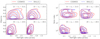 |
Fig. 4. Two-dimensional kernel density plots of morphological parameters in several magnitude bins. The red solid and blue dashed lines denote the training and target samples, respectively. Left panel: the correlation between the size and ellipticity, whilst the right panel presents the correlation between the size and Sérsic index. The plotted contour levels are 20%, 40%, 60%, 80%. |
2.2. Stars: Point objects with synthetic photometry
We treated stars as perfect point objects. Their multi-band photometry was obtained from the population synthesis code, TRILEGAL (Girardi et al. 2005, with version 1.6 and the default model from its website13). We generated six stellar catalogues at galactic coordinates evenly spaced across the KiDS footprint to capture the variation of stellar densities between KiDS tiles. Each catalogue spans 10 deg2. When simulating a specific tile image covering 1 deg2, we selected the stellar catalogue whose central pointing is closest to the target tile, then randomly drew ten per cent of stars from that catalogue as the input. Figure 5 shows the r-band magnitude distributions of the six stellar catalogues compared to the catalogue used by the COllege simulations. The broader coverage of stellar densities is noticeable, marking one of the improvements in SKiLLS. Also, stars in SKiLLS have nine-band magnitudes consistently predicted from a library of stellar spectra (see Girardi et al. 2005, for details), while in COllege, stars only have r-band magnitudes.
 |
Fig. 5. Input magnitude distributions in the r-band for the six stellar catalogues used by SKiLLS. Labels indicate the pointing centres (RA, Dec), except for ‘COllege’, which denotes the stellar catalogue used by K19. |
3. KiDS+VIKING 9-band image simulations
This section details the creation and processing of the multi-band mock images. We start with the creation of KiDS-like optical images (Sect. 3.1) and VIKING-like infrared images (Sect. 3.2), then summarise the SKiLLS fiducial setups in Sect. 3.3. We end the section with the measurement of colours and photometric redshifts (Sect. 3.4).
3.1. KiDS-like optical images
Each KiDS pointing consists of four-band optical images taken with the OmegaCAM camera at the VLT Survey Telescope (Kuijken 2011): u, g, r and i. The r-band images are the primary products used for the shear measurement, while the remaining bands are only for photometric measurements. The science array of the OmegaCAM camera has a ∼1° ×1° field of view covered by 8 × 4 CCD images, each of size 2048 × 4100 pixels with an average resolution of  . Although the CCDs are mounted as closely as possible, a narrow gap between the neighbouring CCDs is technically inevitable. The average gap sizes between the pixels of neighbouring CCDs are:
-
between the long sides of the CCDs: 1.5 mm (100 pixels)
-
central gap along the short sides: 0.82 mm (55 pixels)
-
wide gap along short sides: 5.64 mm (376 pixels).
To avoid ‘dead zones’ caused by these gaps, each tile image incorporates multiple dithered exposures (five in the g, r and i bands, four in the u band). The dithers form a staircase pattern with steps of 25″ in RA and 85″ in declination to match the gaps between CCDs (de Jong et al. 2013).
KiDS raw observations are processed with two independent pipelines: the ASTRO-WISE pipeline designed for the photometric measurements (McFarland et al. 2013; de Jong et al. 2015)14, and the THELI pipeline optimised for the shape measurements (Erben et al. 2005; Schirmer 2013; Kuijken et al. 2015)15. While the former is applied to all four-band observations, the latter is only used for the r-band observations, as KiDS only measures galaxy shapes for lensing in the r-band images. The main difference between the ASTRO-WISE and THELI pipelines is in the co-addition process, where the former resamples all exposures to the same pixel grid with a uniform  pixel size, while the latter preserves the original pixels to maintain image fidelity as much as possible.
We kept all these features in mind when generating SKiLLS optical images. We created raw exposures using the GALSIM pipeline16 (Rowe et al. 2015), with galaxies and stars from the mock catalogues described in Sect. 2. The underlying canvas mimicked the science array of the OmegaCAM camera, including pixels and gaps. Galaxies and stars were mapped to the canvas using the gnomonic (TAN) projection of their original sky coordinates. Following the KiDS image processing, we stacked exposures using the SWARP software (Bertin 2010), with the identical setups as in the KiDS pipelines, including ASTRO-WISE-like images re-gridded to a uniform  pixel size and THELI-like images preserving the original
  pixel size. Figure 6 compares a co-added THELI weight image from SKiLLS to a randomly selected tile from KiDS. It shows that the SKiLLS images contain the main features of KiDS images, including the gaps and dither patterns, albeit lacking subtle features, such as the inhomogeneous backgrounds between CCDs and masks of satellites.
 |
Fig. 6. Comparison of the THELI weight image produced by SKiLLS (left panel) to a randomly selected example from KiDS (right panel). The 8 × 4 CCDs cover a ∼1 square-degree sky area. The shallow regions are caused by the gaps in individual exposures. The same level of agreement is also achieved for the ASTRO-WISE co-added images. |
Besides the image layout, we need information on the pixel noise and point spread function (PSF) to mimic observational conditions. We extracted this information from the fourth public data release of KiDS (KiDS-DR4, or DR4 for short, Kuijken et al. 2019). It has a total of 1006 square-degree survey tiles with stacked ugri images along with their weight maps, masks and source catalogues. We selected a representative sample of 108 tiles and replicated their properties in our image simulations (see Sect. 3.3 for details). For the raw pixel noise, we adopted Gaussian distributions with variances estimated from the ASTRO-WISE weight maps corrected with a boost factor of ∼1.145 (=(0.214/0.2)2) to account for the re-gridding effect. For the PSF, we used two approaches, depending on the different usages of the images.
For the r-band images from which galaxy shapes are measured, we used the position-dependent PSF models for individual exposures. These PSF models, constructed from well-identified stars, are in the form of two-dimensional polynomial functions and can recover a PSF image in the pixel grid for any given image position (see Miller et al. 2013; Kuijken et al. 2015; Giblin et al. 2021 for details). In practice, we recovered 32 PSF images for each exposure using the centre positions of the CCD images. The recovered PSF images contain modelling uncertainties, which can introduce artificial spikes when being used to simulate bright stars. Therefore, we applied a cosine-tapered window to the original PSF image to suppress the modelling noise at its outskirts. The two edges of the window function are defined at 5 and 10 times the full-width half-maximum (FWHM) of the target PSF to preserve features in the central region as much as possible. With these recovered PSF images, we can treat the 32 CCD images separately using their own PSFs, a significant improvement from the constant PSF used in previous work. The recovered PSF image is also superior to a Moffat profile as it captures more delicate features of complex PSFs, such as ellipticity gradients.
For other optical bands where only photometry is measured, we still adopted the Moffat profile, given that the photometric measurement is insensitive to the detailed profile of PSF. We estimated the Moffat parameters by modelling bright stars identified in the ASTRO-WISE images. Since the photometry is measured from the stacked images and is less sensitive to the gentle PSF variation within a given tile, we kept the PSF model invariant for all exposures for simplicity. To alleviate the Moffat fitting bias introduced by the pixelisation of CCD images, we applied the first-order correction to the measured Moffat parameters using image simulations. Specifically, we simulated the pixelated PSF image using measured Moffat parameters and then remeasured them with the same fitting code. The difference between the remeasured and input values is the correction factor and is subtracted from the initially measured value. Our test shows that this correction can suppress the original percent-level bias down to a sub-percent level, which is sufficient for our photometry-related purpose.
3.2. VIKING infrared images
To improve the accuracy of photometric redshifts, KiDS includes near-infrared (NIR) measurements from the VISTA Kilo-degree Infrared Galaxy (VIKING) survey (Edge et al. 2013). The two surveys share an almost identical footprint. We refer to Wright et al. (2019) for details of the VIKING imaging and its usage in KiDS. Briefly, the VIKING data have three levels of products: exposures, paw-prints, and tiles. Given the complex NIR backgrounds, the VIKING survey first takes multiple exposures in quick succession with small jitter steps for reliable estimation of the noisy background. These exposures are then stacked together to create the second level of product: the ‘paw-print’. A paw-print still contains gaps between individual detectors, so six paw-prints with a dither pattern are used to produce a contiguous tile image. However, these co-added tiles have non-contiguous PSF patterns caused by the large dithers between successive paw-prints. Therefore, in the KiDS+VIKING analyses, photometry is done on individual paw-prints instead of the co-added tiles. The dither pattern of paw-prints causes multiple flux measurements per source (typically four in the case of the J-band and two in the other bands). The final flux estimate for each source is a weighted average of the individual measurements with the weights derived from individual flux errors.
Given the complexity of the VIKING observing strategy, we simplified the NIR-band observations in SKiLLS with single images per square degree of KiDS tile. To compensate for the simplified images, we considered the overlap between individual paw-prints when estimating the observational conditions. As we show in Sect. 3.4, this simplified approach can still achieve realistic photometry, which is the only important quality we seek from the NIR-band images.
Specifically, we created a ‘flat-field image’ for each paw-print with the same size and pixel scale. Its pixel value equals the absolute standard deviation of the background pixel values on the corresponding paw-print. For each KiDS pointing, we selected all VIKING paw-prints that overlap in the given one square-degree sky area and stacked their flat-field images with shifts accounting for the different sky pointings of the paw-prints. We took the median pixel value of the co-added flat-field image as the final pixel noise of the corresponding KiDS pointing. In doing so, we captured various overlapping VIKING paw-prints in individual KiDS pointings. Following the typical situations of the KiDS+VIKING data (Wright et al. 2019), we only preserved KiDS pointings with at least two paw-prints in the ZYHKs-bands and at least four paw-prints in the J-band. This requirement reduced the number of pointings from 1006 to 979, which is still plentiful for our purpose. As for the PSF, we employed a constant Moffat profile for each KiDS pointing. The PSF FWHM is a weighted average from overlapping VIKING paw-prints with the weights determined by their noise levels. In order to determine the Moffat concentration index for a given FWHM value, we fitted Moffat profiles to bright stars in some representative paw-prints. The Moffat fitting bias introduced by the pixelisation is corrected using the same method introduced in Sect. 3.1. We found the relationship between the Moffat index n and FWHM (arcsec) in VIKING images to be: ln(n) = 66.56 exp(−6.36 FWHM) + 0.90. This empirical formula is used to pair each FWHM with a unique Moffat index.
3.3. SKiLLS fiducial setup
Since we have 108 deg2 of SHARK galaxies as described in Sect. 2.1, we selected 108 KiDS pointings for the SKiLLS fiducial run. Figure 7 shows the sky locations of the selected 108 tiles along with the 979 KiDS-DR4 tiles that have the nine-band noise and PSF information. Clusters of the selected blocks pair with the six stellar catalogues generated from TRILEGAL so that SKiLLS captures the stellar density variation across the whole KiDS survey (see Sect. 2.2).
 |
Fig. 7. Sky distribution of the KiDS-DR4 tiles. Tiles shown in blue are included in the SKILLS fiducial run (108 tiles); The grey blocks show all KiDS-DR4 tiles that have nine-band noise and PSF information (979 tiles). The black stars indicate the centres of the stellar catalogues generated from TRILEGAL (Girardi et al. 2005). |
Figure 8 compares the r-band noise and PSF properties between the SKiLLS selected tiles and all usable KiDS-DR4 tiles. We measured the PSF size and ellipticity using the weighted quadrupole moments with a circular Gaussian window of dispersion 2.5 pixels, the typical galaxy size in the KiDS sample. The PSF size is defined as
 (4)
(4)
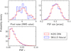 |
Fig. 8. Comparing normalised histograms of the pixel noise (top left), PSF size (top right) and PSF ellipticity (bottom left) between KiDS-DR4 (red) and SKiLLS (blue) for the r-band images. The PSF size and ellipticity are measured from the recovered PSF image using a circular Gaussian window of sigma 2.5 pixels. |
where Qij are the weighted quadrupole moments, and the PSF ellipticity is defined by Eq. (2). Figure 8 shows that the selected tiles represent the KiDS-DR4 data well. Because we vary PSF for individual CCD images and exposures, the 108 SKiLLS images cover 17 280 different PSF models, a significant extension of the 65 PSF models used by FC17 and K19. That also explains the smooth distributions of the PSF parameters. Figure 9 shows similar comparisons for other bands. Again we see fair agreements across all bands. As KiDS-DR4 already covers ∼75% of the whole survey, we expect a similar agreement to the KiDS-Legacy data. The wide coverage of the noise and PSF properties also makes the SKiLLS results more robust than previous simulations and simplifies sensitivity tests (see Sect. 6 for details).
 |
Fig. 9. Comparing normalised histograms of the pixel noise (left) and PSF FWHM (right) between KiDS-DR4 (red) and SKiLLS (blue) for the bands only used for photometry. Equivalent comparisons for the lensing r-band images are presented in Fig. 8. The pixel noise values are divided by the median values in the whole sample for individual bands, so they can be shown in the same range. |
3.4. Photometry and photometric redshifts
With the simulated multi-band images, we can measure colours and estimate photometric redshifts (photo-zs) for simulated galaxies using the same tools developed in KiDS with minor adjustments.
For galaxy colours, we used the GAAP (Gaussian Aperture and PSF) pipeline (Kuijken et al. 2015, 2019). It provides accurate multi-band colours by accounting for PSF differences between filters and optimises signal-to-noise ratio (S/N) by down-weighting the noise-dominated outskirts. The latter is possible because the photo-z estimation only needs the ratio of the fluxes from the same part of a galaxy in the given bands rather than the total light. A prerequisite for the GAAP pipeline is a detection catalogue with source positions and aperture parameters, which we measured from the THELI-like r-band images using the SEXTRACTOR code (Bertin & Arnouts 1996). Once the detection catalogue is ready, we can obtain the list-driven photometry by running the GAAP algorithm on the u, g, r and i ASTRO-WISE-like images and the Z, Y, J, H and Ks simple images. In short, the GAAP method includes three major steps:
-
Homogenising PSFs by convolving the whole image with a spatially variable kernel map modelled from high S/N stars. The resulting image has a simple Gaussian PSF, for which estimating the PSF-independent Gaussian aperture flux is possible. The main side effect is that the convolution process introduces correlated noise between neighbouring pixels, complicating the estimation of measurement uncertainties. GAAP handles this by tracking the noise covariance matrix through the whole process.
-
Defining an elliptical Gaussian aperture function for each source using the size and shape parameters measured by SEXTRACTOR on the r-band detection images. In practice, users must customise the minimum and maximum GAAP aperture sizes to balance the S/N and the effect of blending. Following the KiDS fiducial setup, we set the maximum aperture to 2″ to avoid contamination from neighbouring sources. We conducted two separate runs by setting the minimum aperture to
 and
and  . When used as the input for the photo-z estimation, a source-by-source decision was made to optimise the flux errors across the nine bands (see Kuijken et al. 2019 for details).
 -
Performing the aperture photometry on the PSF-Gaussianised images for each band using the defined aperture functions. It is worth stressing that GAAP aims to provide robust colours for the high S/N parts of galaxies; it underestimates the total fluxes for extended sources by design.
Figure 10 compares the nine-band 1σ GAAP limiting magnitudes between the KiDS-DR4 data and SKiLLS fiducial results. We calculated the median limiting magnitudes for tiles in both KiDS and SKiLLS and then compared their differences. We see a general agreement for all the bands, verifying our noise and PSF modelling. Noticeably, even for the NIR bands where we simplified the VIKING observations with single images, the differences are still tolerable, albeit with larger uncertainties. Figure 11 compares the GAAP photometric distributions between the simulation and data. Once again, we see a decent agreement in both magnitude and colour distributions.
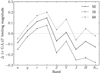 |
Fig. 10. Differences of the image’s median 1σ GAAP limiting magnitudes for the nine bands (simulation – data). The three lines indicate the 16, 50 and 84 percentiles from the 108 tiles included in the SKiLLS fiducial run. The larger scatters in the NIR bands are partially caused by the simplified simulating strategy. |
 |
Fig. 11. Comparison of the GAAP magnitudes (left panel) and colours (right panel) for KiDS-DR4 (red) and SKiLLS (blue). The results include all galaxies with valid photometric measurements (the GAAP flags in nine bands equal to 0). Shape-measurement-related selections are not yet applied. |
For the photo-z estimation, we implemented the public Bayesian Photometric Redshift (BPZ; Benítez 2000) code with the re-calibrated template set from Capak (2004) and the Bayesian redshift prior from Raichoor et al. (2014). We closely followed the settings in the KiDS-DR4 analysis (Kuijken et al. 2019) unless it conflicts with the simulation input. For example, we set ZMAX to 2.5, the limiting redshift of SKiLLS galaxies, instead of 7.0 as in the data. We tested the choice of ZMAX in the simulations and found that only 0.1% of the test sample resulted in estimates differing more than 0.1, which means most of the objects have similar photo-z estimates and end up in the same tomographic bins for these two choices. Moreover, the SHARK photometry in the u, g, r, i and Z bands is based on the Sloan Digital Sky Survey (SDSS) photometric system, which is slightly different from the KiDS/VIKING system (Kuijken et al. 2019). We corrected these slight differences in the measured GAAP magnitudes in order to use the KiDS/VIKING filters to run the BPZ code. The detailed procedures and comparisons are described in Appendix C. Overall, the modification is minor and has a negligible impact on the magnitude, colour distributions, and final shear biases. Still, it improves the agreement between the simulation and the data in the photo-z distributions. Unless specified otherwise, we base our fiducial results on the transformed photometry.
Figure 12 compares the estimated photo-z to the true redshift from the input SURFS-SHARK simulations in several measured magnitude bins. It shows the photo-z vs. true redshift distributions, along with annotated statistics based on the distributions of (zB − ztrue)/(1 + ztrue)≡Δz/(1 + z) values. We see the BPZ code works well in SKiLLS and is at the same level as in KiDS (Wright et al. 2019). More detailed verification of the SKiLLS photo-z performance is presented in the companion redshift calibration paper (van den Busch et al., in prep.).
 |
Fig. 12. Photometric redshifts vs. true redshifts in several apparent r-band magnitude bins. The annotated statistics are: the normalised median-absolute-deviation (σm) of the quantity Δz/(1 + z), the fraction of sources with |Δz/(1 + z)| > 3σm (η3) and the fraction of sources with |Δz/(1 + z)| > 0.15 (ζ0.15). The dashed lines correspond to the one-to-one relation, and the dotted lines show |Δz/(1 + z)| = σm. |
As for the redshift calibration, our end-to-end approach, which starts with image simulation followed by object detection, PSF homogenisation, forced multi-band photometry, and photo-z estimation, is a significant improvement compared to previous catalogue-level simulations (e.g. Hoyle et al. 2018; van den Busch et al. 2020; DeRose et al. 2022). The image-simulation-based approach not only yields more realistic observational uncertainties but also naturally accounts for the blending effect, which is hard to address at the catalogue level. As for the shear calibration, these photo-z estimates are essential for performing tomographic selections (K19). Our approach that directly measures the photo-zs from simulated images accounts for various measurement uncertainties of photo-zs, hence a tomographic selection consistent with how it is done in the data. Moreover, using the same mock catalogue in both shear and redshift calibration unites these two long-separated processes in the KiDS-Legacy analysis.
4. Shape measurements with the updated lensfit
The primary task of any weak lensing survey is to measure the shapes of galaxy images. Previous KiDS analyses tackled this task using a likelihood-based code, dubbed lensfit (Miller et al. 2007, 2013; Kitching et al. 2008). It is the default shape measurement algorithm for the KiDS-Legacy analysis, with some updates described in this section. We test SKiLLS using this updated lensfit code17.
4.1. The self-calibration version of lensfit
The lensfit code, first developed for CFHTLenS (Heymans et al. 2012), follows a Bayesian model-fitting approach. We refer to Miller et al. (2013) for its detailed formalism. In brief, it first performs a joint fit to individual exposures using a PSF-convolved galaxy model, which yields a likelihood distribution of seven parameters: 2D position, flux, scalelength, bulge-to-total flux ratio and complex ellipticity. Then it deduces the ellipticity parameters from the likelihood-weighted mean values by marginalising other parameters with priors as described by Miller et al. (2013). For each ellipticity estimate, an inverse-variance weight is also determined from (Miller et al. 2013)
![Mathematical equation: $$ \begin{aligned} { w}_i \equiv \left[ \frac{\sigma _{\epsilon ,\ i}^2\ \epsilon _{\rm max}^2}{\epsilon _{\rm max}^2-2\sigma _{\epsilon ,\ i}^2} + \sigma _{\epsilon ,\ \mathrm{pop}}^2 \right]^{-1}, \end{aligned} $$](/articles/aa/full_html/2023/02/aa45210-22/aa45210-22-eq14.gif) (5)
(5)
where σϵ, i is the uncertainty of the measured ellipticity, σϵ, pop is the ellipticity dispersion of the galaxy population (intrinsic shape noise), and ϵmax is the maximum allowed ellipticity in the lensfit model-fitting. As for KiDS data, we adopted σϵ, pop = 0.253 and ϵmax = 0.804.
The code has evolved as KiDS progressed. The most significant is a self-calibration scheme for noise bias, as detailed in FC17. The pixel noise in a given image skews the likelihood, which biases the estimate of individual galaxy ellipticities. It is a complex function of the signal-to-noise ratio, galaxy properties and PSF morphology, making it difficult to predict accurately. Thus, lensfit conducts an approximate correction using the measurements themselves, that is a self-calibration. The basic idea is to simulate a test galaxy with parameters measured from the first run, then remeasure the test galaxy using the same pipeline. The difference between the remeasured and input values serves as a correction factor for the corresponding parameter. Since its introduction, self-calibration has been a standard part of lensfit, given its promising overall performance (Mandelbaum et al. 2015; FC17; K19). We keep this feature for the KiDS-Legacy analysis.
4.2. Updates for KiDS-Legacy analysis
A long-standing mystery of all previous lensfit analyses has been the presence of a small but significant residual bias in ϵ2 that is uncorrelated with the PSF and the underlying shear (Miller et al. 2013; Hildebrandt et al. 2016; Giblin et al. 2021). We now understand that this feature arises from an anisotropic error in the original likelihood sampler, which has been corrected in our algorithm. However, we found that this correction inadvertently increases the fraction of residual PSF contamination in the weighted average signal (see the discussion in Giblin et al. 2021). Besides, object selection and galaxy weights are also known to introduce bias (e.g. Kaiser 2000; Bernstein & Jarvis 2002; Hirata & Seljak 2003; Jarvis et al. 2016 and FC17). These selection biases can be more severe than the raw measurement bias and hence cannot be ignored even for a perfect self-calibration measurement algorithm.
FC17 presented a method to isotropise weights using an empirical correction scheme, which has been adopted in previous KiDS studies to mitigate these biases. Unfortunately, we found this approach to be insufficient for the improved lensfit algorithm. Furthermore, we found the approach to be sensitive to the sample volume, and therefore hard to apply consistently to the data and simulations. So, we introduce a new empirical correction scheme that mitigates the PSF contamination to the weighted shear signal.
4.2.1. Weight correction
We start with the PSF leakages in the reported weight. For galaxies with comparable surface brightness, those aligned with the PSF tend to have a higher integrated signal-to-noise ratio than those cross-aligned with the PSF. This orientation preference causes the asymmetry of the measurement variance (the  term in Eq. (5)), which can be measured using a linear function to the first order
![Mathematical equation: $$ \begin{aligned} S_i = \alpha _{S}\epsilon _{\mathrm{PSF},\ i,\ \mathrm{proj}} + \mathcal{N} \left[\langle S\rangle ,\ \sigma _S\right], \end{aligned} $$](/articles/aa/full_html/2023/02/aa45210-22/aa45210-22-eq16.gif) (6)
(6)
where  refers to the measurement variance, and
  is the scalar projection of the PSF ellipticity in the direction of the galaxy ellipticity. The αS term quantifies the PSF contamination in the measurement variance, while 𝒩[⟨S⟩, σS] denotes the noise, which we assume follows a Gaussian distribution with a mean of ⟨S⟩ and standard deviation of σS.
Following FC17, we estimate the PSF contamination as a function of the integrated signal-to-noise ratio (νSN) reported by lensfit and the resolution, which is defined as
 (7)
(7)
where  is the circularised galaxy size with re and q denoting the scalelength along the major axis and the axis ratio, respectively. The PSF size rPSF is defined by Eq. (4). By construction, the resolution ℛ has a value between 0 and 1, with a larger value corresponding to a more poorly resolved object.
When estimating αS, we first divide galaxies into an irregular 20 × 20 grid of νSN and ℛ, each containing the same number of objects. Then in each bin, we perform a linear regression using Eq. (6) to measure αS. Figure 13 shows the measurements for the KiDS-DR4 re-run with the updated lensfit. It demonstrates a clear correlation between the estimated αS and the νSN and ℛ. We derive the corrected measurement variance for individual galaxies through  , where the value of αS is determined based on which νSN-ℛ bin the target galaxy is assigned to. The corrected lensfit weight is then calculated with
![Mathematical equation: $$ \begin{aligned} { w}_{\mathrm{corr},\ i} \equiv \left[ \frac{\sigma ^2_{\epsilon ,\ i,\ \mathrm{corr}}\ \epsilon _{\rm max}^2}{\epsilon _{\rm max}^2-2\sigma ^2_{\epsilon ,\ i,\ \mathrm{corr}}} + \sigma _{\epsilon ,\ \mathrm{pop}}^2 \right]^{-1}, \end{aligned} $$](/articles/aa/full_html/2023/02/aa45210-22/aa45210-22-eq22.gif) (8)
(8)
 |
Fig. 13. PSF leakage in the measurement variance as a function of S/N and ℛ. We note that the larger ℛ corresponds to a poorer resolution by definition (Eq. (7)). |
following Eq. (5). We verified that this approach is sufficient to remove the overall weight bias and is robust against the binning scheme.
4.2.2. Ellipticity correction
In addition to the weight bias, there is still some residual PSF leakage in the measured ellipticity because of the residual noise bias and selection effects. To first order, this residual PSF bias can be formulated as
![Mathematical equation: $$ \begin{aligned} {\boldsymbol{\epsilon }}_{\mathrm{obs},\ i} = {\boldsymbol{\epsilon }}_{\mathrm{true},\ i} + {\boldsymbol{\alpha }}\ {\boldsymbol{\epsilon }}_{\mathrm{PSF},\ i} + {\boldsymbol{c}} + \mathcal{N} \left[0,\ {\boldsymbol{\sigma }}_{\epsilon }\right], \end{aligned} $$](/articles/aa/full_html/2023/02/aa45210-22/aa45210-22-eq23.gif) (9)
(9)
where ϵobs, i is the measured ellipticity, ϵtrue, i is the underlying true ellipticity, α is the fraction of the PSF ellipticity ϵPSF, i that leaks into the measured ellipticity, and c is an additive term uncorrelated with the PSF. 𝒩[0, σϵ] denotes the noise in individual shape measurements, which are assumed to follow a Gaussian distribution of mean 0 and standard variation σϵ. We note that all parameters in Eq. (9) are complex numbers (α = α1 + iα2). We focus on the α term, as the c term with the improved likelihood sampler is now small in practice, and the 𝒩[0, σϵ] vanishes for an ensemble of galaxies.
Like the weight bias correction, we first estimate α in the 20 × 20 grid of νSN and ℛ using a linear regression of Eq. (9). Figure 14 shows the amplitude of α in the 2D νSN and ℛ plane. We see modest values in most situations, except for the low νSN cases, where it drops abruptly to negative values. We confirmed that the negative tail is mainly from the selection effects by measuring the PSF leakage using the input ellipticity in simulations. This non-trivial negative tail prevents us from using the direct correction approach introduced in the weight bias correction section. Therefore, we propose a hybrid approach, with a fitting procedure for the overall trend and a direct correction for residuals. Specifically, we first fit the measured α as a function of νSN and ℛ, using a function of the form
 (10)
(10)
 |
Fig. 14. PSF leakage in the measured ellipticity after the weight calibration as a function of S/N and ℛ. We note that the larger ℛ corresponds to a poorer resolution by definition (Eq. (7)). |
whose coefficients are constrained using the weighted mean results from the 20 × 20 grid. Then, we correct the raw measurements of individual galaxies using ϵobs, i, tmp = ϵobs, i − αp(νSN, i, ℛi) ϵPSF, i, where the polynomial αp(νSN, i, ℛi) is determined from the target galaxy’s νSN, i and ℛi. After removing the overall trend, we use the corrected ϵobs, i, tmp to measure the residual αr, which changes mildly across the 2D νSN and ℛ plane. Therefore, we can conduct the direct correction through ϵobs, i, corr = ϵobs, i, tmp − αrϵPSF, i, where the values of αr for individual galaxies are determined based on which νSN–ℛ bin they are assigned. This two-step approach balances performance and robustness. We verified that the corrected measurements have negligible PSF leakages and the results are robust against the binning scheme.
4.3. Comparison between KiDS and SKiLLS
We applied the updated lensfit code to KiDS-DR4 and SKiLLS r-band images. The object selections after the measurements are detailed in Appendix D. In short, we largely followed the selection criteria proposed in Hildebrandt et al. (2017), with an additional resolution cut introduced to mitigate the PSF contamination. We applied the same selections to the KiDS data and SKiLLS simulated catalogue to ensure a consistent selection effect, even though SKiLLS does not contain artefacts like asteroids and binary stars.
Figure 15 compares the weighted distributions of some critical observables reported by the updated lensfit. The SKiLLS results match the KiDS-DR4 data reasonably well. We also checked the properties of the close pairs. Specifically, we show the magnitude difference and the projected distance between close pairs in the measured catalogues. Both properties agree well between the data and simulations, implying SKiLLS has realistic clustering features. These realistic neighbouring properties are essential for an accurate shear calibration, especially when considering the shear interference between blended objects (see Sect. 5 for details).
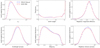 |
Fig. 15. Comparison of the updated lensfit measurements between KiDS (red) and SKiLLS (blue). All distributions are normalised with lensfit weights, except for the distribution of lensfit weight itself. The neighbour properties are based on the nearest neighbour found in the measured catalogue. The magnitude difference is defined as the neighbour magnitude minus the magnitude of the primary target. The lack of close pairs with distance below ∼1 arcsec is due to the conservative blending cut used by KiDS (see Appendix D). This cut helps to mitigate the worst of the blending bias. |
5. Shear biases for the updated lensfit
The central task of image simulations is to quantify the average shear bias for a selected source sample. This is done by comparing the inferred shear γobs, to the input shear γinput, which have a linear correlation to the first order (Heymans et al. 2006)
 (11)
(11)
where m is known as the multiplicative bias, and c is the additive bias. The simulation-based calibration focuses on the multiplicative bias, as the additive bias is usually corrected empirically (for example, the correction scheme proposed in Sect. 4.2). So we use the term ‘shear bias’ and ‘multiplicative bias’ interchangeably throughout the paper. We note that all parameters in Eq. (11) are in complex forms, such as m = m1 + im2. However, we found m1 and m2 to be consistent in our analysis, so unless specified, we only report the amplitude m.
The shear calibration methodology keeps evolving as our understanding of systematics deepens. Early studies demonstrated that the shear bias correlated with galaxy properties and PSFs, especially the signal-to-noise ratio and resolution (e.g. Miller et al. 2013; Hoekstra et al. 2015; Mandelbaum et al. 2018; Samuroff et al. 2018). So the first lesson is to avoid using one averaged result from the whole simulation as a scalar calibration to the entire data unless the simulations perfectly represent the data. A natural procedure then attempts to estimate the shear bias as a function of the galaxy and PSF properties (e.g. Miller et al. 2013; Jarvis et al. 2016). Nevertheless, we can only derive the relation of the bias to the noisy, measured properties, as the true properties are unknown in actual data. FC17 found that the relation derived from the measured properties introduces biases because of the correlations between observed quantities, an effect referred to as the ‘calibration selection bias’. So the second lesson is that we should be cautious about object-based shear calibrations that rely on the relation to the noisy properties. That is why the recent simulations try to resemble the data and only provide a mean correction for an ensemble of galaxies (e.g. K19). The latest lesson, stressed by MacCrann et al. (2022), is the interplay between shear estimates of blended objects at different redshifts, a higher-order effect that the traditional constant shear simulations cannot capture. It becomes more important as the precision of surveys improves.
Our shear calibration method builds on all these lessons. We created constant shear simulations following the previous KiDS tomographic calibration method but with improvements to the photo-z estimates by taking advantage of the simulated multi-band images (Sect. 5.1). Using additional blending-only variable shear simulations, we applied a correction to account for the interplay between blends containing different shears (Sect. 5.2). When testing the PSF modelling algorithm in image simulations, we detected a small but noticeable change of shear bias, which was also corrected in our fiducial results (Sect. 5.3).
5.1. Results from the constant shear simulations
Our constant shear simulations largely followed FC17 and K19 with some simplifications for better usage of computational resources. Table 1 lists the main changes we made compared to our predecessor. Given the 108 deg2 of unique synthetic galaxies we built in Sect. 2, we mimicked 108 KiDS pointings, where we vary the PSF, noise level and stellar density as detailed in Sect. 3. To reduce the shape noise, we copied each tile image with galaxies rotated by 90 degrees. We created four sets of constant shear simulations with input shear: (0.0283, 0.0283), (0.0283, −0.0283), ( − 0.0283, −0.0283), ( − 0.0283, 0.0283). The total simulated area is 864 (=108 × 4 × 2) deg2, which is equivalent to ∼5170 deg2 after accounting for the shape noise cancellation (=864 × (σϵ, raw/σϵ, SNC)2, where σϵ, raw and σϵ, SNC denote the weighted dispersion of the mean input ellipticities before and after the shape noise cancellation), which is roughly four times the final KiDS-Legacy area.
For a tomographic analysis, we need to estimate the bias for each redshift bin separately, given that the galaxy properties vary between bins. This requires photo-z estimates for the simulated galaxies. For SKiLLS, we can follow the KiDS processing steps to directly measure photo-zs, thanks to the simulated nine-band images. We conducted the detection from the THELI-like r-band images, the PSF Gaussianisation and forced multi-band photometry using the GAAP pipeline, and the photo-z estimates with the BPZ code (see Sect. 3.4 for details). This consistent data processing ensures that SKiLLS embraces realistic photometric properties, marking one of the most significant improvements over the previous image simulations.
As shown in Fig. 15, SKiLLS matches KiDS generally well but not perfectly. K19 argued that an accurate estimate of the shear bias must account for any mismatches between the simulations and the target data. Therefore, we followed FC17 and K19 to reweight the simulation estimates using the lensfit reported νSN and resolution factor ℛ (Eq. (7)). Specifically, for each tomographic bin, we first divided simulated galaxies into 20 × 20 bins of νSN and ℛ, each containing equal lensfit weight. Then we estimated the multiplicative bias for each νSN–ℛ bin using Eq. (11). Galaxies in the target data were assigned the bias based on the νSN–ℛ bin they fall in, and the final bias for each tomographic bin was the lensfit-weighted average of these individual assignments. This procedure ensures the estimated bias accounts for any νSN and ℛ differences between the simulations and the data while also minimising the impact of the calibration selection bias.
Table 2 and Fig. 16 show the multiplicative bias estimates for the KiDS-DR4 re-run with the updated lensfit from our constant shear simulations. The quoted errors only contain the statistical uncertainties from the linear fitting. Compared to Table 2 of K19, we reduced the statistical uncertainties by about half because of the larger sky area simulated. Direct comparisons between the calibration values quoted in Table 2, cannot be made to those in K19 and Giblin et al. (2021). We updated the shape measurement algorithm lensfit and calibrated the raw measurement against PSF contamination in our analysis (see Sect. 4.2). These changes modify the effective size and signal-to-noise ratio distribution of the samples and hence the overall calibration in each tomographic bin. Furthermore, Giblin et al. (2021) accounts for the Wright et al. (2020) ‘gold’ selection for photometric redshifts, which reduces the effective number density by ∼20%, compared to the sample simulated in this analysis.
 |
Fig. 16. Multiplicative bias as a function of tomographic bins for KiDS-DR4 with the updated lensfit. The red diamonds indicate our final results with the corrections for the shear-interplay effect (Sect. 5.2) and PSF modelling bias (Sect. 5.3), whilst the grey points are the raw results from the idealised constant shear simulations (Sect. 5.1). The hatched regions indicate the nominal error budgets proposed for comparison (see Sect. 6 for details). |
Shear bias for the six tomographic bins.
5.2. Impact of blends at different redshifts
MacCrann et al. (2022) recently highlighted a complication that arises from blended objects at different redshifts, which are, therefore, sheared by different amounts. It stems from the fact that when objects are blended, a shear measurement of one object responds to the shear of the neighbouring object. This higher-order effect, which we refer to as ‘shear interplay’ through this paper, cannot be captured by the aforementioned constant shear simulations. So, we built an extra suite of variable shear simulations to account for this effect.
Since the shear interplay only happens when objects are blended, we built a blending-only input catalogue for these additional simulations to save some computing time. This blending-only catalogue only contains bright galaxies with bright neighbours, assuming that the blending effects caused by the faint objects are sufficiently accounted for by our main constant shear simulations, which include galaxies down to magnitude 27. It means we only ignore the higher-order shear-interplay effect from the faint objects, which is valid as long as the excluded faint galaxies are below the measurement limit of the survey. In practice, we selected all galaxies with an input r-band magnitude < 25. The choice of this magnitude cut meets the overall sensitivity of the KiDS survey. We further discarded those isolated galaxies whose nearest neighbour is 4″ away based on their input positions. The final selected sample covers ∼10% of the entire input catalogue. But after the lensfit measurements, this blending-only simulation covers ∼35% of the objects measured in the whole simulation (see Table 2 for the exact values). The higher fraction in the measured catalogue is because most objects fainter than 25 in the r-band magnitude are not measurable for KiDS.
To properly account for the shear-interplay effect, we need realistic shear fields with proper correlations between the shear and the environment of galaxies. We refer to Appendix E for technical details of our approach to creating such variable shear fields. In short, we considered two primary contributions to the weak lensing signal: the cosmic shear due to the large-scale structure and the tangential shear induced by the foreground objects (also known as the galaxy-galaxy lensing effect). The cosmic shear was learned from the MICE Grand Challenge (MICE-GC) simulation (Fosalba et al. 2015b), whilst the tangential shear was calculated analytically by assuming Navarro-Frenk-White (Navarro et al. 1995) density profiles for the underlying dark matter halos. Figure 17 shows the average shear signals as a function of redshift. We see a roughly linear relationship between the mean signals and redshift. On average, the cosmic shear contributes more than the tangential shear. However, we note that the importance of the tangential shear varies between systems depending on the host halo mass of the foreground galaxies.
 |
Fig. 17. Variable shear field as a function of redshift. The solid black line shows the mean amplitude of the final used shears, which contain two components: the cosmic shear (dashed magenta line) and the tangential shear (dotted orange line). We refer to Appendix E for details. |
To increase the constraining power, we used 32 variable shear fields generated from the same learning algorithm but with different choices for the direction of the shear. Specifically, we created four variable shear fields with directions of the cosmic shear that differ by 90°. Then, we made eight copies for each shear field by rotating the final shear by 45° each time. We also created an extra suite of blending-only constant shear simulations to serve as a reference. The final sky area of these additional simulations is 7776 deg2(=108 × 36 × 2). Except for the input shear, these blending-only simulations use the same pipeline, observational conditions and random seeds as the full simulations detailed in Sect. 5.1 so that we can directly correct the constant shear results using the extra bias estimated from these additional simulations.
While estimating the shear bias for constant shear simulations is straightforward by directly conducting the linear least squares fitting to all measurements using Eq. (11), given that the input shear values do not depend on the underlying sample. The situation is more complicated for variable shear simulations. The crucial caveat is that the shear bias is now correlated with redshift [ ] due to the shear-interplay effect. Owing to the realistic shear field we built, we can measure
  directly from simulations by performing the least squares fitting to sub-samples of galaxies split based on their true redshift. The same approach can also be applied to the blending-only constant shear simulations to get
  ; only, in that case, we would expect a negligible correlation with the true redshift, except for some fluctuations stemming from the different signal-to-noise ratios between true redshift bins. Figure 18 shows the difference
  , which is a direct measure of the impact of the shear-interplay effect, as the only difference between the simulations is the input shear value. It demonstrates evident residuals that correlate with redshift, indicating the non-trivial impact of the shear-interplay effect. Interestingly, the high-redshift outliers, which have an estimated photo-z much lower than their true redshifts, show the most noticeable residuals across all tomographic bins, implying that the blends with objects from different redshifts are likely responsible for those outliers. This coupling between the photo-z and shear biases in blended systems warrants a dedicated future study.
 |
Fig. 18. Residual shear bias introduced by the shear-interplay effect (orange points) as a function of the true redshift estimated from the blending-only simulations. The residuals are calculated from |


To correct the raw shear bias derived in Sect. 5.1, we need an average correction  , which integrates over ztrue as
  , where n(ztrue) is the weighted number density with respect to redshift (the dashed lines shown in Fig. 18). The average results for individual tomographic bins are shown in Table 2 and Fig. 19. In practice, we should also account for the blending fraction, which is correlated with the signal-to-noise ratio and resolution, as is the bias itself. Therefore, we perform the correction in each νSN–ℛ bin, following the binning strategy proposed for reweighting the simulation (see Sect. 5.1). Specifically, for each νSN–ℛ bin, we estimate the average correction
  and the blending fraction. The blending fraction is estimated as the ratio of the effective number counts between the blending-only simulation and the whole simulation. Then, we shift the raw bias in each νSN–ℛ bin with the product of
  and blending fraction. The final corrected bias is the lensfit-weighted average of these shifted biases. This correction process can be easily combined with the reweighting procedure, as they use the same binning strategy.
 |
Fig. 19. Mean residual multiplicative bias introduced by the shear-interplay effect. It is calculated from |

Another more direct way to inspect the blending effect is to check the relation between the shear bias and the nearest neighbour distance in the input catalogue. Figure 20 demonstrates such estimations for both constant shear and variable shear simulations. We see a clear correlation between the bias and the neighbour distance in both simulations, indicating the significant impact of the blending effect. It also confirms our choice of 4″ to define blended systems, as we barely see any correlation after this threshold. The other important finding is that the traditional constant shear simulations can already capture the dominant contributions from the blending effect. The higher-order impact we study in this section, shown as the bias difference between the variable shear and constant shear simulations, contributes relatively minor except for the very close blends. The aggressive treatment of the blending in lensfit can partially explain this finding, as it throws away most of the recognised blends (Hildebrandt et al. 2017).
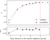 |
Fig. 20. Multiplicative bias as a function of the nearest neighbour distance. The distance is measured in the input catalogue after removing faint galaxies whose r-band input magnitude > 25. The x-axis values correspond to the weighted average of each sub-sample selected to estimate the multiplicative bias shown on the y-axis. Top panel: the individual biases measured from the blending-only variable shear simulations (magenta points) and the blending-only constant shear simulations (dark green points). The vertical dashed lines show the threshold we set when building the blending-only simulations. Two extra dark green points beyond the threshold are calculated from the full constant shear simulations. Bottom panel: the difference between these two estimates (varShear – constShear). |
We note that our variable shear simulations and the correction methodology differ from those of MacCrann et al. (2022). In their study, the simulated shear changes as a function of redshift, but, per redshift slice, it remains constant across the field of view. The chosen redshift intervals and adjusted shear have no physical meaning in their setups. But they built four sets of simulations by choosing different redshift intervals, so they were able to fit a smooth model to the simulated results, obtaining a continuous redshift-bias relation. In our approach, we computed the variable shear fields using a more physical model that accounts for the shear correlations to both the redshift and clustering of galaxies (see Appendix E). Thanks to these realistic shear fields, we can measure the redshift-bias relation directly from the simulations without additional model fitting procedures. Our direct measurements confirmed the non-trivial impact of the shear-interplay effect (see Fig. 18). By design, our method results in large uncertainties for low redshift bins due to the small input shear values. Fortunately, these low redshift bins carry little cosmic shear signals, making the overall downgrade tolerable. Albeit following a different approach, our final result is consistent with MacCrann et al. (2022) finding that the overall correction due to the shear-interplay effect is negligible for the current weak lensing surveys. However, it will potentially impact the next-generation surveys.
5.3. PSF modelling bias
So far, we have ignored the PSF modelling errors, given the expected accuracy of PSF models relative to the requirement of the current weak lensing surveys (see e.g. Giblin et al. 2021). We used the input PSF for shape measurements (i.e. assuming perfect PSF modelling). However, as the requirement of systematics becomes more stringent, it becomes necessary to check the impact of PSF modelling errors. This section quantifies this impact by including the PSF modelling procedure in the simulations.
The SKiLLS images have realistic stellar populations and variable PSFs across the field, so we can apply the PSF modelling code directly to the simulated images using similar setups as for the data. We refer to Kuijken et al. (2015) for detailed descriptions of the PSF modelling algorithm used by KiDS. In short, it describes the position-dependent PSFs at the detector resolution using a set of amplitudes on a 48 × 48 pixel grid. The spatial variation of each pixel value is fitted with a two-dimensional polynomial of order n, with additional flexibility for allowing the lowest order coefficients to differ from CCD to CCD. This extra freedom allows for a more complex PSF variation between CCDs and, in principle, allows for discontinuities in the PSF between adjacent CCDs. When fitting to individual stars, the flux and centroid of each star are allowed to change, and a sinc function interpolation is used to align the PSF model with the star position. Following Giblin et al. (2021), we set n = 4 and allow the polynomial coefficients up to order 1 to vary between CCDs. We skipped the complicated star-galaxy separation procedure with an implicit assumption that the point-source sample used by KiDS is sufficiently pure as verified using NIR colours in Giblin et al. (2021). Instead, we built a perfect star sample by cross-matching the detected catalogue with the input star catalogue. However, we still applied the same magnitude and signal-to-noise ratio cuts as used in the data to ensure a similar noise level in the modelled stars.
We selected 30 tiles from the available 108 fiducial tiles to test the influence of PSF modelling uncertainty on the multiplicative bias. These selected tiles cover the whole range of the PSF size, including the minimum and maximum. We performed the PSF modelling on the selected tiles and re-ran lensfit using the modelled PSFs. Since all the images and detection catalogues are unchanged, the shift of the shear bias directly quantifies the contribution of the PSF modelling errors. Figure 21 and Table 2 show the shifts for the six tomographic bins. We find the PSF modelling procedure does introduce small yet noticeable biases. Our fiducial results take these additional biases into account.
 |
Fig. 21. Changes in multiplicative bias when modelled PSFs are used instead of the input PSFs. The hatched regions indicate the nominal error budgets proposed for comparison (see Sect. 6 for details). |
5.4. Results
The final results after accounting for both the shear-interplay effect and PSF modelling errors are listed as mfinal in Table 2 and shown as the red points in Fig. 16. Within the current statistical uncertainties, the average shifts due to the shear-interplay effect and PSF modelling errors are insignificant across all redshift bins, as indicated in Fig. 16 between the grey points and the red points. A more noticeable change is the increased uncertainty introduced by the correction of the shear-interplay effect, especially in the low redshift bins where the input shear values are overall small in the variable shear simulations. Our proposed systematic error budgets account for these additional uncertainties (the hatched regions in Fig. 16).
6. Sensitivity analysis
Given the resemblance between the SKiLLS and KiDS images and the reweighting in the signal-to-noise ratio and ℛ when estimating the shear biases, it is reasonable to assume that the estimates from SKiLLS can be used to correct the actual measurements. Nevertheless, it is still worth testing the robustness of SKiLLS results and accounting for any potential systematic uncertainties. We start with tests proposed by FC17 and K19 in Sect. 6.1. Thanks to the broad coverage of observational conditions in SKiLLS, we can quickly achieve these analyses without dedicated test runs. Additionally, we test how sensitive the lensfit results are to the changes in the input galaxy morphology (Sect. 6.2). For comparison reasons, we propose some nominal error budgets based on the general performance of SKiLLS and the overall requirements of lensing analyses with KiDS. Specifically, we set an error budget of 0.02 for the first and sixth tomographic bins and 0.01 for the remaining bins. We found these nominal error budgets are conservative enough that our results are robust within them. Nevertheless, we note that these nominal error budgets can be over-conservative for cosmic shear analyses. In which case, we can estimate more accurate systematic uncertainties following other more aggressive approaches proposed by previous KiDS analyses (Giblin et al. 2021; Asgari et al. 2021).
6.1. Impact of observational conditions
When developing SKiLLS, we improved most of the critical sources of uncertainty in the previous KiDS simulations. For instance, we based our input galaxy catalogue on N-body simulations, so it has reasonable clustering features and is complete down to 27 in the r-band magnitude. We learned realistic morphologies from observations using a powerful technique, dubbed vine copulas, which captures the multi-dimensional correlations between ellipticities and other galaxy properties. We included six stellar catalogues to account for the varying stellar densities across the survey sky. We covered more variations of the PSF models and background noise levels. Above all, we measured photo-zs directly from the simulated multi-band images to properly account for the correlation between the measurement uncertainties on the redshift and shear estimates. Consequently, most of the sensitivity analyses proposed by FC17 and K19 are either trivial or redundant for the SKiLLS results.
Still, we examine the robustness of the lensfit results against some crucial properties by comparing between sub-samples. The basic idea is to split the fiducial simulations into three sub-samples based on a targeted property and examine the consistency of their bias estimates to the fiducial results. These sub-samples contain roughly equal numbers of measured objects while covering different ranges of the targeted property. After applying the overall shear correction from the whole sample to the sub-samples, we calculate their residual biases to quantify the impact of the variations of the targeted property. We note that the estimated residuals are not systematic biases in our fiducial results, but they indicate the robustness of the shape measurement algorithm against the tested properties. Ideally, if the simulations fully match the data in the distributions of the targeted property, we would still expect an accurate bias estimate even if the estimated residuals are large. For that account, the estimated residuals are conservative upper limits of the systematic biases in our results.
Figure 22 shows the estimated residuals for the variations in four critical properties of the simulated images: the PSF ellipticity, PSF size, background noise level in r-band images, and stellar density. It indicates that our fiducial results are robust within the nominal error budgets, considering the shifts shown in the plots are the upper limits of possible deviations.
 |
Fig. 22. Changes in multiplicative bias when the fiducial simulations are divided into three sub-samples containing different observational conditions. From the left- to right-hand panels and top to bottom panels, the four panels show the results when splitting based on the PSF ellipticity, PSF size, background noise level in r-band images and stellar density. The hatched regions indicate the nominal error budgets proposed for comparison (see Sect. 6 for details). We note that the shifts correspond to the upper limits of potential systematic biases in our results (see Sect. 6.1 for details). |
6.2. Impact of the input galaxy morphology
We learned the galaxy morphology from Griffith et al. (2012) based on Sérsic models fitted to the HST observations. We have shown that our copula-based learning algorithm captures the properties of the reference sample (see Sect. 2.1.2). However, the reference sample itself contains measurement errors. This section examines how sensitive the lensfit measurements are to the changes in the input galaxy morphology.
We focus on the three morphological parameters used to describe the Sérsic profile: the half-light radius, axis ratio and Sérsic index. To get some indication of the overall accuracy of the reference sample, we first checked the fitting uncertainties. We found that the median relative uncertainties for these three parameters are ≲5%, ≲5% and ≲10%, respectively. We took these values (quoted as σ below) as the benchmark for changing the input galaxy morphology. We built new input catalogues by increasing a certain parameter with 1σ, 2σ and 3σ each time while keeping the other parameters unchanged. We generated test simulations using these new input catalogues and measured the bias difference with respect to the fiducial simulations.
Figure 23 presents the test results from 10 tiles of simulations. We find minor residuals in most cases, with the most significant shifts seen when changing the Sérsic index. We note that we shifted all galaxies with the same amount of fractions, resulting in an overall shift of the whole distribution, as shown in the bottom panels of Fig. 23. Given that the entire distribution’s uncertainty is much smaller than the individual measurement uncertainties, we are testing the most extreme cases. Hence, the measured residuals only indicate the sensitivity of lensfit towards the input galaxy properties but cannot be seen as systematics in our fiducial results. To achieve tighter requirements for future surveys, we will need a shape measurement method that is less susceptible to the galaxy properties, as the fidelity of image simulations will always be limited by the realism of the input galaxy catalogue. For the upcoming KiDS-Legacy analysis, we will, therefore, also explore an alternative method based on the METACALIBRATION technique (Huff & Mandelbaum 2017; Sheldon & Huff 2017), which is expected to be more robust against the galaxy properties (Yoon et al., in prep.).
 |
Fig. 23. Changes in multiplicative bias when the morphological parameters of all input galaxies are increased by a certain fraction. Top panels: the shifts of the multiplicative bias caused by changing morphological parameter values. The three shift points correspond to the increased factor of 1 + 1σ (dark red), 1 + 2σ (dark orange) and 1 + 3σ (dark green), where σ denotes the median relative uncertainties reported by Griffith et al. (2012; σ = 5%,5%,10% for the half-light radius, the axis ratio and Sérsic index, respectively). The hatched regions indicate the nominal 0.01 error budget for comparison. Bottom panels: the normalised histograms comparing before and after changing morphological parameter values. We note that we shifted all galaxies by the same fraction, resulting in an overall shift of the whole distribution, which corresponds to the most extreme cases, as the uncertainty on the entire distribution is much smaller than on individual values. |
7. Discussion and conclusions
An unbiased measurement of the ensemble shear signal is the backbone of reliable precision cosmology with weak lensing surveys. The state-of-the-art shape measurement methods have already reached a percent, if not a sub-percent, level of accuracy. But meanwhile, the statistical powers of weak lensing surveys keep growing, thus putting more stringent requirements on the systematics. Higher-order effects distinct from the shape estimation bias start drawing more and more attention, including the selection bias, PSF modelling errors and shear-interplay bias, which are challenging to eliminate by only improving the shape measurement algorithms. On the other hand, image simulations show promising performance in calibrating these higher-order effects.
This paper presents the third-generation image simulations for the KiDS survey, dubbed SKiLLS, after SCHOol (FC17) and COllege (K19). The current image simulations implemented several significant developments to meet the calibration requirement of the KiDS-Legacy analysis, which uses an updated lensfit. First and foremost, we simulated the full nine-band images and produced a self-consistent joint shear-redshift mock catalogue. We combined the cosmological simulations with deep imaging observations as input to balance the sample volume and the realism of the galaxy morphology. We also improved the realism of images by varying PSFs between CCDs, including stellar density variations and varying noise levels between pointings. We followed the whole KiDS procedure for the photometric measurements, including the r-band detection, PSF Gaussianisation, forced multi-band photometry and photo-z estimates. Given the large volume of simulated galaxies and their realistic photometric properties, the joint shear-redshift mock catalogue not only improves the shear calibration but also benefits the redshift calibration (van den Busch et al., in prep.).
We further explored the impact of blends of galaxies at different redshifts by building realistic shear fields accounting for the redshift and clustering of galaxies. We accounted for the PSF modelling errors by conducting the PSF modelling procedures on the image simulations. Finally, we performed a series of sensitivity tests, including changing the input galaxy properties, demonstrating robustness in the SKiLLS measured calibration values for future lensing studies with KiDS. The final shear calibration results for the updated lensfit are summarised in Table 2 and shown in Fig. 16. Our statistical uncertainties and sensitivity tests suggest that the shear bias estimated from SKiLLS is robust within the nominal error budget of 0.02 for the first and sixth tomographic bins and 0.01 for the remaining bins. Besides, we share some lessons and findings that can be instructive for calibrating future weak lensing surveys.
The fidelity of image simulations relies heavily on the realism of the input galaxy population in terms of photometry, morphology, and clustering. Therefore, the latest image simulations have used high-quality imaging observations as the input. But, this observation-based input is limited by its sample volume and depth, which will soon be inadequate for the next generation of weak lensing surveys. An alternative is to acquire the input galaxy population from cosmological simulations. However, the cosmological simulations still cannot fully reproduce the observed galaxy morphology – the first-order feature that cannot be compromised in image simulations. In our work, we show that it is possible to keep the merits from both sides by integrating cosmological simulations with high-quality imaging observations. We proposed a copula-based learning algorithm that can mimic and link the observed morphology to synthetic galaxies from cosmological simulations. Our results suggest that this hybrid approach is promising for future image simulations that require a large volume of galaxies.
Recent studies have already pointed out that the shear calibration must consider redshift-related selections, which requires simulating multi-band observations to account for the measurement of photo-zs (e.g. K19, MacCrann et al. 2022). We further show that multi-band image simulations with a sufficiently large volume of galaxies benefit not only the shear calibration but also the redshift calibration. It allows us to perform the whole procedure for photometric measurements, ensuring realistic photometric properties in the mock catalogue. This end-to-end approach is a significant improvement compared to previous catalogue-level simulations (e.g. Hoyle et al. 2018; van den Busch et al. 2020; DeRose et al. 2022). Moreover, image simulations allow us to study the blending effect in redshift estimates, which are otherwise hard to consider at the catalogue level. Given the importance of blending, we argue that unifying the shear and redshift calibrations with multi-band image simulations will be crucial for future high-accuracy tomographic analysis.
MacCrann et al. (2022) recently studied the impact of blended systems that contain galaxies experiencing different shears, an effect we referred to as ‘shear interplay’ throughout the paper. We extended their study by building realistic variable shear fields accounting for both redshift and clustering of galaxies. We also explicitly included the contribution from galaxy-galaxy lensing. Our final results confirmed its overall minor impact on current weak lensing surveys (see Fig. 16). However, we measured an evident redshift-bias correlation from our blending-only variable shear simulations, proving the presence of the shear-interplay effect and its non-trivial contributions (see Fig. 18). We also found that the photo-z outliers showcase the most significant shear interplay, implying a common cause of the shear and redshift biases. A dedicated study is warranted to further explore this coupling in blended systems, as it will soon be relevant for the next-generation weak lensing surveys.
Image simulations usually skip the PSF modelling process, given the PSF validation conducted in data (see e.g. Giblin et al. 2021). Thanks to the realistic SKiLLS images, we can test the impact of the PSF modelling errors by directly running the PSF modelling code in simulated images. By comparing the shear biases measured from runs with and without PSF modelling, we identified sub-percent residual biases from the PSF modelling errors. Although this is insignificant for the current requirement, it will concern future weak lensing surveys. Therefore, we stress the importance of improving or including the PSF modelling algorithm in image simulations for future surveys.
Finally, we tested the sensitivity to the properties of the input galaxy population. By changing the input values of morphological parameters, we found that our current fiducial shape measurement method, lensfit, is sensitive to the input galaxy shapes but within a tolerable level for KiDS analysis. Still, we will develop an alternative method based on the METACALIBRATION technique (Huff & Mandelbaum 2017; Sheldon & Huff 2017) for KiDS-Legacy analysis, which is more robust against the galaxy properties (Yoon et al., in prep.). It will be essential for future weak lensing surveys to develop such a method that is less sensitive to the galaxy properties, as the image simulations will never fully represent the observed galaxy population given the limits of its input catalogue.
Strictly speaking, the expectation value of the ellipticity is γ/(1 − κ), where κ is the convergence. But as κ ≪ 1 in the weak lensing regime, we can safely neglect this term.
Nevertheless, we note that SKiLLS can also calibrate other algorithms, such as the KiDS METACALIBRATION catalogue (Yoon et al., in prep.).
Acknowledgments
We thank Fedor Getman for providing the deep VST-COSMOS catalogue and Arun Kannawadi for reading the manuscript and providing useful comments. We also wish to thank other members of the KiDS-Legacy Calibration Working Group (especially Benjamin Joachimi, Benjamin Stölzner and Anna Wittje) for informative discussions and suggestions through numerous teleconferences. This work used the compute resources from the Academic Leiden Interdisciplinary Cluster Environment (ALICE) provided by Leiden University. We acknowledge support from: the Netherlands Research School for Astronomy (SSL); the Royal Society and Imperial College (KK); the Netherlands Organisation for Scientific Research (NWO) under Vici grant 639.043.512 (HHo); and the UK Science and Technology Facilities Council (STFC) under grant ST/N000919/1 (LM) and ST/V000594/1 (CH). We also acknowledge support from the European Research Council (ERC) under grant agreement No. 647112 (CH) and No. 770935 (HHi, JLvdB, AHW); the Max Planck Society and the Alexander von Humboldt Foundation in the framework of the Max Planck-Humboldt Research Award endowed by the Federal Ministry of Education and Research (CH, MY); the Deutsche Forschungsgemeinschaft Heisenberg grant Hi 1495/5-1 (HHi); the Polish National Science Center through grants no. 2020/38/E/ST9/00395, 2018/30/E/ST9/00698, 2018/31/G/ST9/03388 and 2020/39/B/ST9/03494 (MBi); the Polish Ministry of Science and Higher Education through grant DIR/WK/2018/12 (MBi); the University of Western Australia through a Scholarship for International Research Fees and Ad Hoc Postgraduate Scholarship (MBr); and the ARC Centre of Excellence for All Sky Astrophysics in 3 Dimensions (ASTRO 3D) through project number CE170100013 (CL). The results in this paper are based on observations made with ESO Telescopes at the La Silla Paranal Observatory under programme IDs: 088.D-4013, 092.A-0176, 092.D-0370, 094.D-0417, 177.A-3016, 177.A-3017, 177.A-3018 and 179.A-2004, and on data products produced by the KiDS consortium. The KiDS production team acknowledges support from: Deutsche Forschungsgemeinschaft, ERC, NOVA and NWO-M grants; Target; the University of Padova, and the University Federico II (Naples). Contributions to the data processing for VIKING were made by the VISTA Data Flow System at CASU, Cambridge and WFAU, Edinburgh. The SURFS-SHARK simulations were produced at the Pawsey Supercomputing Centre with funding from the Australian Government and the Government of Western Australia. Author contributions: All authors contributed to the development and writing of this paper. The authorship list is given in three groups: the lead authors (SSL, KK, HHo, LM) followed by two alphabetical groups. The first alphabetical group includes those who are key contributors to both the scientific analysis and the data products. The second group covers those who have either made a significant contribution to the data products, or to the scientific analysis.
References
- Aas, K., Czado, C., Frigessi, A., & Bakken, H. 2009, Insurance: Mathematics and Economics, 44, 182 [CrossRef] [Google Scholar]
- Abbott, T. M. C., Aguena, M., Alarcon, A., et al. 2022, Phys. Rev. D, 105, 023520 [CrossRef] [Google Scholar]
- Aihara, H., Arimoto, N., Armstrong, R., et al. 2018, PASJ, 70, S4 [NASA ADS] [Google Scholar]
- Alarcon, A., Gaztanaga, E., Eriksen, M., et al. 2021, MNRAS, 501, 6103 [NASA ADS] [CrossRef] [Google Scholar]
- Asgari, M., Lin, C.-A., Joachimi, B., et al. 2021, A&A, 645, A104 [NASA ADS] [CrossRef] [EDP Sciences] [Google Scholar]
- Bartelmann, M. 1996, A&A, 313, 697 [NASA ADS] [Google Scholar]
- Bartelmann, M., & Schneider, P. 2001, Phys. Rep., 340, 291 [Google Scholar]
- Bedford, T., & Cooke, R. M. 2002, Ann. Stat., 30, 1031 [CrossRef] [Google Scholar]
- Benítez, N. 2000, ApJ, 536, 571 [Google Scholar]
- Bernstein, G. M., & Armstrong, R. 2014, MNRAS, 438, 1880 [NASA ADS] [CrossRef] [Google Scholar]
- Bernstein, G. M., & Jarvis, M. 2002, AJ, 123, 583 [NASA ADS] [CrossRef] [Google Scholar]
- Bertin, E. 2010, Astrophysics Source Code Library [record ascl:1010.068] [Google Scholar]
- Bertin, E., & Arnouts, S. 1996, A&AS, 117, 393 [NASA ADS] [CrossRef] [EDP Sciences] [Google Scholar]
- Bravo, M., Lagos, C. d. P., Robotham, A. S. G., Bellstedt, S., & Obreschkow, D. 2020, MNRAS, 497, 3026 [NASA ADS] [CrossRef] [Google Scholar]
- Bridle, S., Balan, S. T., Bethge, M., et al. 2010, MNRAS, 405, 2044 [NASA ADS] [Google Scholar]
- Cañas, R., Elahi, P. J., Welker, C., et al. 2019, MNRAS, 482, 2039 [CrossRef] [Google Scholar]
- Capak, P. L. 2004, Ph.D. Thesis, University of Hawai’i [Google Scholar]
- Cappellaro, E., Botticella, M. T., Pignata, G., et al. 2015, A&A, 584, A62 [NASA ADS] [CrossRef] [EDP Sciences] [Google Scholar]
- Carretero, J., Castander, F. J., Gaztañaga, E., Crocce, M., & Fosalba, P. 2015, MNRAS, 447, 646 [NASA ADS] [CrossRef] [Google Scholar]
- Carretero, J., Tallada, P., Casals, J., et al. 2017, in Proceedings of the European Physical Society Conference on High Energy Physics, 5-12 July, 488 [CrossRef] [Google Scholar]
- Chang, C., Jarvis, M., Jain, B., et al. 2013, MNRAS, 434, 2121 [NASA ADS] [CrossRef] [Google Scholar]
- Chauhan, G., Lagos, C. d. P., Obreschkow, D., et al. 2019, MNRAS, 488, 5898 [NASA ADS] [CrossRef] [Google Scholar]
- Coe, D., Benítez, N., Sánchez, S. F., et al. 2006, AJ, 132, 926 [Google Scholar]
- Crocce, M., Castander, F. J., Gaztañaga, E., Fosalba, P., & Carretero, J. 2015, MNRAS, 453, 1513 [NASA ADS] [CrossRef] [Google Scholar]
- Czado, C. 2019, in Analyzing Dependent Data with Vine Copulas: A Practical Guide with R (Cham: Springer International Publishing AG) [CrossRef] [Google Scholar]
- Czekaj, M. A., Robin, A. C., Figueras, F., Luri, X., & Haywood, M. 2014, A&A, 564, A102 [NASA ADS] [CrossRef] [EDP Sciences] [Google Scholar]
- Damjanov, I., Zahid, H. J., Geller, M. J., Fabricant, D. G., & Hwang, H. S. 2018, ApJS, 234, 21 [NASA ADS] [CrossRef] [Google Scholar]
- Dark Energy Survey Collaboration (Abbott, T., et al.) 2016, MNRAS, 460, 1270 [Google Scholar]
- Davies, L. J. M., Driver, S. P., Robotham, A. S. G., et al. 2015, MNRAS, 447, 1014 [Google Scholar]
- Davies, L. J. M., Robotham, A. S. G., Driver, S. P., et al. 2018, MNRAS, 480, 768 [NASA ADS] [CrossRef] [Google Scholar]
- Dawson, W. A., Schneider, M. D., Tyson, J. A., & Jee, M. J. 2016, ApJ, 816, 11 [Google Scholar]
- De Cicco, D., Paolillo, M., Falocco, S., et al. 2019, A&A, 627, A33 [NASA ADS] [CrossRef] [EDP Sciences] [Google Scholar]
- de Jong, J. T. A., Verdoes Kleijn, G. A., Kuijken, K. H., & Valentijn, E. A. 2013, Exp. Astron., 35, 25 [Google Scholar]
- de Jong, J. T. A., Verdoes Kleijn, G. A., Boxhoorn, D. R., et al. 2015, A&A, 582, A62 [NASA ADS] [CrossRef] [EDP Sciences] [Google Scholar]
- DeRose, J., Wechsler, R. H., Becker, M. R., et al. 2022, Phys. Rev. D, 105, 123520 [NASA ADS] [CrossRef] [Google Scholar]
- Duffy, A. R., Schaye, J., Kay, S. T., & Dalla Vecchia, C. 2008, MNRAS, 390, L64 [Google Scholar]
- Dunkley, J., Komatsu, E., Nolta, M. R., et al. 2009, ApJS, 180, 306 [NASA ADS] [CrossRef] [Google Scholar]
- Edge, A., Sutherland, W., Kuijken, K., et al. 2013, The Messenger, 154, 32 [NASA ADS] [Google Scholar]
- Elahi, P. J., Welker, C., Power, C., et al. 2018, MNRAS, 475, 5338 [NASA ADS] [CrossRef] [Google Scholar]
- Elahi, P. J., Cañas, R., Poulton, R. J. J., et al. 2019a, PASA, 36, e021 [NASA ADS] [CrossRef] [Google Scholar]
- Elahi, P. J., Poulton, R. J. J., Tobar, R. J., et al. 2019b, PASA, 36, e028 [CrossRef] [Google Scholar]
- Erben, T., Schirmer, M., Dietrich, J. P., et al. 2005, Astron. Nachr., 326, 432 [NASA ADS] [CrossRef] [Google Scholar]
- Euclid Collaboration (Martinet, N., et al.) 2019, A&A, 627, A59 [NASA ADS] [CrossRef] [EDP Sciences] [Google Scholar]
- Euclid Collaboration (Guglielmo, V., et al.) 2020, A&A, 642, A192 [NASA ADS] [CrossRef] [EDP Sciences] [Google Scholar]
- Fenech Conti, I., Herbonnet, R., Hoekstra, H., et al. 2017, MNRAS, 467, 1627 [NASA ADS] [Google Scholar]
- Fosalba, P., Crocce, M., Gaztañaga, E., & Castander, F. J. 2015a, MNRAS, 448, 2987 [NASA ADS] [CrossRef] [Google Scholar]
- Fosalba, P., Gaztañaga, E., Castander, F. J., & Crocce, M. 2015b, MNRAS, 447, 1319 [NASA ADS] [CrossRef] [Google Scholar]
- Fukugita, M., Ichikawa, T., Gunn, J. E., et al. 1996, AJ, 111, 1748 [Google Scholar]
- Giblin, B., Heymans, C., Asgari, M., et al. 2021, A&A, 645, A105 [NASA ADS] [CrossRef] [EDP Sciences] [Google Scholar]
- Girardi, L., Groenewegen, M. A. T., Hatziminaoglou, E., & da Costa, L. 2005, A&A, 436, 895 [NASA ADS] [CrossRef] [EDP Sciences] [Google Scholar]
- González-Fernández, C., Hodgkin, S. T., Irwin, M. J., et al. 2018, MNRAS, 474, 5459 [Google Scholar]
- Griffith, R. L., Cooper, M. C., Newman, J. A., et al. 2012, ApJS, 200, 9 [NASA ADS] [CrossRef] [Google Scholar]
- Hamana, T., Shirasaki, M., Miyazaki, S., et al. 2020, PASJ, 72, 16 [Google Scholar]
- Hartlap, J., Hilbert, S., Schneider, P., & Hildebrandt, H. 2011, A&A, 528, A51 [NASA ADS] [CrossRef] [EDP Sciences] [Google Scholar]
- Hasinger, G., Capak, P., Salvato, M., et al. 2018, ApJ, 858, 77 [Google Scholar]
- Heymans, C., Van Waerbeke, L., Bacon, D., et al. 2006, MNRAS, 368, 1323 [Google Scholar]
- Heymans, C., Van Waerbeke, L., Miller, L., et al. 2012, MNRAS, 427, 146 [Google Scholar]
- Heymans, C., Tröster, T., Asgari, M., et al. 2021, A&A, 646, A140 [NASA ADS] [CrossRef] [EDP Sciences] [Google Scholar]
- Hildebrandt, H., Choi, A., Heymans, C., et al. 2016, MNRAS, 463, 635 [Google Scholar]
- Hildebrandt, H., Viola, M., Heymans, C., et al. 2017, MNRAS, 465, 1454 [Google Scholar]
- Hirata, C., & Seljak, U. 2003, MNRAS, 343, 459 [Google Scholar]
- Hoekstra, H., & Jain, B. 2008, Ann. Rev. Nucl. Part. Sci., 58, 99 [NASA ADS] [CrossRef] [Google Scholar]
- Hoekstra, H., Herbonnet, R., Muzzin, A., et al. 2015, MNRAS, 449, 685 [NASA ADS] [CrossRef] [Google Scholar]
- Hoekstra, H., Viola, M., & Herbonnet, R. 2017, MNRAS, 468, 3295 [NASA ADS] [CrossRef] [Google Scholar]
- Hoyle, B., Gruen, D., Bernstein, G. M., et al. 2018, MNRAS, 478, 592 [Google Scholar]
- Hu, W. 1999, ApJ, 522, L21 [Google Scholar]
- Huff, E., & Mandelbaum, R. 2017, ArXiv e-prints [arXiv:1702.02600] [Google Scholar]
- Huterer, D. 2002, Phys. Rev. D, 65, 063001 [Google Scholar]
- Ivezić, Ž., Kahn, S. M., Tyson, J. A., et al. 2019, ApJ, 873, 111 [Google Scholar]
- Jarvis, M., Sheldon, E., Zuntz, J., et al. 2016, MNRAS, 460, 2245 [Google Scholar]
- Joe, H. 2014, in Dependence Modeling with Copulas (CRC Press) [CrossRef] [Google Scholar]
- Kaiser, N. 1992, ApJ, 388, 272 [Google Scholar]
- Kaiser, N. 2000, ApJ, 537, 555 [NASA ADS] [CrossRef] [Google Scholar]
- Kannawadi, A., Hoekstra, H., Miller, L., et al. 2019, A&A, 624, A92 [NASA ADS] [CrossRef] [EDP Sciences] [Google Scholar]
- Kilbinger, M. 2015, Rep. Prog. Phys., 78, 086901 [Google Scholar]
- Kitching, T. D., Miller, L., Heymans, C. E., van Waerbeke, L., & Heavens, A. F. 2008, MNRAS, 390, 149 [Google Scholar]
- Kitching, T. D., Balan, S. T., Bridle, S., et al. 2012, MNRAS, 423, 3163 [Google Scholar]
- Komatsu, E., Dunkley, J., Nolta, M. R., et al. 2009, ApJS, 180, 330 [NASA ADS] [CrossRef] [Google Scholar]
- Kuijken, K. 2011, The Messenger, 146, 8 [NASA ADS] [Google Scholar]
- Kuijken, K., Heymans, C., Hildebrandt, H., et al. 2015, MNRAS, 454, 3500 [Google Scholar]
- Kuijken, K., Heymans, C., Dvornik, A., et al. 2019, A&A, 625, A2 [NASA ADS] [CrossRef] [EDP Sciences] [Google Scholar]
- Lagos, C. d. P., Tobar, R. J., Robotham, A. S. G., et al. 2018, MNRAS, 481, 3573 [CrossRef] [Google Scholar]
- Lagos, C. d. P., Robotham, A. S. G., Trayford, J. W., et al. 2019, MNRAS, 489, 4196 [NASA ADS] [CrossRef] [Google Scholar]
- Laigle, C., McCracken, H. J., Ilbert, O., et al. 2016, ApJS, 224, 24 [Google Scholar]
- Lange, R., Moffett, A. J., Driver, S. P., et al. 2016, MNRAS, 462, 1470 [NASA ADS] [CrossRef] [Google Scholar]
- Laureijs, R., Amiaux, J., Arduini, S., et al. 2011, ArXiv e-prints [arXiv:1110.3193] [Google Scholar]
- Le Fèvre, O., Cassata, P., Cucciati, O., et al. 2013, A&A, 559, A14 [Google Scholar]
- Le Fèvre, O., Tasca, L. A. M., Cassata, P., et al. 2015, A&A, 576, A79 [Google Scholar]
- MacCrann, N., Becker, M. R., McCullough, J., et al. 2022, MNRAS, 509, 3371 [Google Scholar]
- Mandelbaum, R. 2018, ARA&A, 56, 393 [Google Scholar]
- Mandelbaum, R., Rowe, B., Armstrong, R., et al. 2015, MNRAS, 450, 2963 [Google Scholar]
- Mandelbaum, R., Lanusse, F., Leauthaud, A., et al. 2018, MNRAS, 481, 3170 [NASA ADS] [CrossRef] [Google Scholar]
- Massey, R., Heymans, C., Bergé, J., et al. 2007, MNRAS, 376, 13 [Google Scholar]
- Massey, R., Hoekstra, H., Kitching, T., et al. 2013, MNRAS, 429, 661 [Google Scholar]
- Masters, D. C., Stern, D. K., Cohen, J. G., et al. 2017, ApJS, 841, 111 [NASA ADS] [Google Scholar]
- Masters, D. C., Stern, D. K., Cohen, J. G., et al. 2019, ApJ, 877, 81 [Google Scholar]
- McConnell, N. J., & Ma, C.-P. 2013, ApJ, 764, 184 [Google Scholar]
- McCracken, H. J., Milvang-Jensen, B., Dunlop, J., et al. 2012, A&A, 544, A156 [NASA ADS] [CrossRef] [EDP Sciences] [Google Scholar]
- McFarland, J. P., Verdoes-Kleijn, G., Sikkema, G., et al. 2013, Exp. Astron., 35, 45 [Google Scholar]
- Melchior, P., & Viola, M. 2012, MNRAS, 424, 2757 [Google Scholar]
- Miller, L., Kitching, T. D., Heymans, C., Heavens, A. F., & van Waerbeke, L. 2007, MNRAS, 382, 315 [Google Scholar]
- Miller, L., Heymans, C., Kitching, T. D., et al. 2013, MNRAS, 429, 2858 [Google Scholar]
- Navarro, J. F., Frenk, C. S., & White, S. D. M. 1995, MNRAS, 275, 720 [NASA ADS] [CrossRef] [Google Scholar]
- Navarro, J. F., Frenk, C. S., & White, S. D. M. 1996, ApJ, 462, 563 [Google Scholar]
- Navarro, J. F., Frenk, C. S., & White, S. D. M. 1997, ApJ, 490, 493 [Google Scholar]
- Obreschkow, D., Klöckner, H. R., Heywood, I., Levrier, F., & Rawlings, S. 2009, ApJ, 703, 1890 [Google Scholar]
- Paulin-Henriksson, S., Amara, A., Voigt, L., Refregier, A., & Bridle, S. L. 2008, A&A, 484, 67 [NASA ADS] [CrossRef] [EDP Sciences] [Google Scholar]
- Planck Collaboration XIII. 2016, A&A, 594, A13 [NASA ADS] [CrossRef] [EDP Sciences] [Google Scholar]
- Poulton, R. J. J., Robotham, A. S. G., Power, C., & Elahi, P. J. 2018, PASA, 35, e042 [NASA ADS] [CrossRef] [Google Scholar]
- Raichoor, A., Mei, S., Erben, T., et al. 2014, ApJ, 797, 102 [Google Scholar]
- Refregier, A. 2003, ARA&A, 41, 645 [NASA ADS] [CrossRef] [Google Scholar]
- Refregier, A., Kacprzak, T., Amara, A., Bridle, S., & Rowe, B. 2012, MNRAS, 425, 1951 [Google Scholar]
- Robin, A. C., Reylé, C., Derrière, S., & Picaud, S. 2003, A&A, 409, 523 [NASA ADS] [CrossRef] [EDP Sciences] [Google Scholar]
- Robotham, A. S. G., Bellstedt, S., Lagos, C. d. P., et al. 2020, MNRAS, 495, 905 [NASA ADS] [CrossRef] [Google Scholar]
- Rowe, B. T. P., Jarvis, M., Mandelbaum, R., et al. 2015, Astron. Comput., 10, 121 [Google Scholar]
- Samuroff, S., Bridle, S. L., Zuntz, J., et al. 2018, MNRAS, 475, 4524 [NASA ADS] [CrossRef] [Google Scholar]
- Schirmer, M. 2013, ApJS, 209, 21 [NASA ADS] [CrossRef] [Google Scholar]
- Sérsic, J. L. 1963, Bol. Asoc. Argent. Astron. Plata Argent., 6, 41 [Google Scholar]
- Sheldon, E. S., & Huff, E. M. 2017, ApJ, 841, 24 [NASA ADS] [CrossRef] [Google Scholar]
- Silverman, J. D., Kashino, D., Sanders, D., et al. 2015, ApJS, 220, 12 [NASA ADS] [CrossRef] [Google Scholar]
- Sklar, M. 1959, Publ. Inst. Stat. Univ. Paris, 8, 229 [Google Scholar]
- Spergel, D., Gehrels, N., Baltay, C., et al. 2015, ArXiv eprints [arXiv:1503.03757] [Google Scholar]
- Stanford, S. A., Masters, D., Darvish, B., et al. 2021, ApJS, 256, 9 [NASA ADS] [CrossRef] [Google Scholar]
- Tallada, P., Carretero, J., Casals, J., et al. 2020, Astron. Comput., 32, 100391 [Google Scholar]
- van den Busch, J. L., Hildebrandt, H., Wright, A. H., et al. 2020, A&A, 642, A200 [NASA ADS] [CrossRef] [EDP Sciences] [Google Scholar]
- van den Busch, J. L., Wright, A. H., Hildebrandt, H., et al. 2022, A&A, 664, A170 [NASA ADS] [CrossRef] [EDP Sciences] [Google Scholar]
- van der Wel, A., Noeske, K., Bezanson, R., et al. 2016, ApJS, 223, 29 [Google Scholar]
- Viola, M., Cacciato, M., Brouwer, M., et al. 2015, MNRAS, 452, 3529 [NASA ADS] [CrossRef] [Google Scholar]
- Wright, C. O., & Brainerd, T. G. 2000, ApJ, 534, 34 [Google Scholar]
- Wright, A. H., Driver, S. P., & Robotham, A. S. G. 2018, MNRAS, 480, 3491 [Google Scholar]
- Wright, A. H., Hildebrandt, H., Kuijken, K., et al. 2019, A&A, 632, A34 [NASA ADS] [CrossRef] [EDP Sciences] [Google Scholar]
- Wright, A. H., Hildebrandt, H., van den Busch, J. L., & Heymans, C. 2020, A&A, 637, A100 [NASA ADS] [CrossRef] [EDP Sciences] [Google Scholar]
Appendix A: An empirical modification to the synthetic photometry
We detail the proposed empirical modification of the SHARK photometry in this appendix. It intends to improve the agreement of the magnitude counts between the simulations and observations, which is critical for the redshift and shear calibrations.
We took the COSMOS2015 catalogue as the benchmark under an implicit assumption that the COSMOS field is representative. The COSMOS2015 catalogue is a near-infrared-selected photometric catalogue containing 30-band photometry, precise photometric redshifts and stellar masses for more than half a million objects (Laigle et al. 2016). We note that measurement uncertainties and modelling errors are inevitable for observations, especially for faint objects. Therefore, the COSMOS2015 catalogue cannot, in principle, be treated as the truth. Nevertheless, these uncertainties are tolerable for calibrating a KiDS-like sample. Following this reasoning, we tuned the simulated properties solely based on the COSMOS2015 measurements for the sake of simplicity, but caution any physical interpretation of our modified results.
First of all, we must locate the cause of the discrepancy. As the SHARK free parameters were tuned using the observed stellar mass functions, we would expect the number density of the SHARK galaxies is realistic. This is confirmed by Figure A.1, where we see a good agreement of the stellar mass distributions between the data and simulations. As a next step, we inspected the stellar mass-to-light ratio (Υ⋆), for which took the Ks-band photometry as an indicator of the total luminosity as it is least affected by the dust extinctions. Figure A.2 shows the comparing results as a function of the stellar mass in several redshift bins. Noticeably, the SHARKΥ⋆ is systematically higher than the COSMOS2015 one, especially in the low stellar mass and low redshift ranges. It can, at least partially, explain the discrepancy seen in the magnitude distributions. Fortunately, this Υ⋆ difference is easy to calibrate without changing other intrinsic properties, such as the colours, redshifts, and positions.
 |
Fig. A.1. Comparison of the stellar mass functions. For the COSMOS2015 catalogue (red solid lines), we use the median values of the marginalised likelihood distributions. For the SHARK catalogue (green dashed lines), we assume that the total stellar mass equals the sum of the stellar masses in the bulge and the disc. |
We, therefore, conducted an empirical modification of the simulated magnitudes to account for the Υ⋆ difference. We divided SHARK and COSMOS2015 galaxies into 24 × 23 evenly spaced small bins based on their redshifts and stellar masses. In each bin, we calculated the median Υ⋆ for the SHARK and COSMOS2015 galaxies, separately. To mitigate the observational uncertainties, we only used the COSMOS2015 galaxies with good stellar mass estimations (δM⋆ < 0.15M⋆). For bins that lack observations, we extrapolated Υ⋆, obs as a function of M⋆ for each redshift slice. After inspecting the general trend, we found a good fit by combining an exponential descending function in the low M⋆ end and a linear ascending function in the high M⋆ end. From these estimates, we constructed a magnitude modification factor Δmag as
![Mathematical equation: $$ \begin{aligned} \Delta \mathrm{mag} = -2.5\log _{10}\left(\frac{\mathrm{median}[\Upsilon _{\star ,\ \mathrm{Shark }}]}{\mathrm{median}[\Upsilon _{\star ,\ \mathrm{obs}}]}\right)\ . \end{aligned} $$](/articles/aa/full_html/2023/02/aa45210-22/aa45210-22-eq40.gif) (A.1)
(A.1)
Figure A.3 demonstrates the estimated Δmag values in the 2D redshift-stellar mass plane. Following the difference seen in Fig. A.2, substantial modifications happen in the low mass and low redshift bins. Therefore, the magnitude modification reduces the range of magnitudes of SHARK galaxies. We note that the different bands share the same Δmag values, so the colours of individual galaxies are preserved.
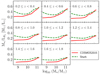 |
Fig. A.2. Ks-band stellar mass-to-light ratio as a function of stellar mass. The red and green lines correspond to the COSMOS2015 and SHARK galaxies, respectively. |
 |
Fig. A.3. Distribution of the magnitude modification factor Δmag in the redshift-stellar mass plane. The red colour denotes negative values, whilst the blue colour denotes positive values. The definition of Δmag is shown in Eq. A.1. For a given galaxy, the same Δmag value is added to the apparent magnitudes for all available bands. |
Appendix B: Modelling multivariate distributions with vine copulas
We outline some necessary background on the vine-copula modelling in this appendix. For a comprehensive introduction, we refer to Joe (2014) and Czado (2019).
A copula is simply a multivariate cumulative distribution function (CDF) with uniformly distributed margins. The Sklar (1959) theorem states that any d-dimensional CDF F(x), with univariate margins F1(x1),...,Fd(xd), can be described as F(x) = C1, ..., d(F1(x1),...,Fd(xd)), where C1, ..., d is the corresponding copula function. Therefore, given a joint probability distribution function (PDF) f(x) with d-dimensional variables x = (x1, ..., xd), we can always find a copula density c1, ..., d that is the partial differentiation of the copula C1, ..., d, such that
 (B.1)
(B.1)
It means we can divide the modelling of any joint multi-dimensional PDF into two parts: one for the independent distributions of the individual random variables {fi(xi)}, and the other for their mutual dependence captured by the copula density c1, ..., d(F1(x1),...,Fd(xd)).
The restriction of the classical copula method is that most of the flexible copula families available in the literature are bivariate, making it tricky to deal with high-dimensional distributions. In this aspect, the vine copula method stands out as an effective approach (Bedford & Cooke 2002; Aas et al. 2009). A vine copula is a graphical model organising a set of bivariate copulas, called pair-copulas. The chain rule states that any PDF f(x) can be decomposed as
 (B.2)
(B.2)
with f(.|.) being the conditional PDF. Aas et al. (2009) further states that each term in Eq. (B.2) can be decomposed into an appropriate pair-copula times a conditional marginal density as described by the following general formula
 (B.3)
(B.3)
where v stands for a d-dimensional vector, vj is an arbitrary component of v, and v−j denotes the v-vector excluding this component. Therefore, the multiple dependence can be captured by a product of pair-copulas acting on underlying conditional probability distributions. Since the decomposition shown in Eq. (B.2) is not unique, there is a significant number of possible pair-copula constructions. These possibilities are organised by the graphical models, that is the vines.
Appendix C: Transformation of the SDSS filters to the KiDS/VIKING filters
This appendix details the transformation of the Sloan Digital Sky Survey (SDSS) photometric system to the KiDS/VIKING system. The SDSS photometric system comprises five colour bands (u, g, r, i, z) that cover wavelengths ranging from ultra-violet at 3000 Å to near-infrared at 11 000 Å (Fukugita et al. 1996), whilst the KiDS/VIKING system contains optical filters (u, g, r, i) mounted on the VST OmegaCAM camera (Kuijken 2011) and near-infrared filters (Z, Y, J, H, Ks) mounted on the VISTA infrared camera (González-Fernández et al. 2018). Figure C.1 compares the filter curves from these two systems. The differences are noticeable, especially for the Z filter, where the KiDS/VIKING system cuts the tail towards long wavelengths. We used the following relation to correct these differences:
 (C.1)
(C.1)
 |
Fig. C.1. Comparison of the normalised transmission curves of the ugriZ filters in the SDSS photometric system (red solid lines) and the KiDS/VIKING system (green dashed lines). |
where X corresponds to the target filter, whilst W is another filter, helping to define the colour. Given the superior depth of the r-band measurement, we picked it as the Y filter whenever possible. When the r band is the target filter, we chose the g band as the Y filter. The coefficients j(ztrue) and h(ztrue) are correlated with the redshift, for which we took values from the PROSPECT web-portal18. For the redshift, we used the true redshift from the input SURFS-SHARK simulations.
As for the SKiLLS measured photometry, we need to correct six measurements: the five u-, g-, r-, i-, Z-band magnitudes measured in the ASTRO-WISE images (MAG_GAAP_X) and the r-band magnitudes measured in the THELI images (MAG_AUTO). There is no need to correct the remaining YJHKs bands as SKiLLS also uses VISTA filters for them. Figure C.2 shows the distributions of the magnitude modification as a function of the initially measured magnitude. The modifications are generally small, especially for the u and g bands. Even for the r and Z bands with the most significant differences, the majority of objects has a modification ≲0.05. Accordingly, the changes in the overall magnitude and colour distributions are negligible. Still, we get a better agreement with the data in the photo-z distributions after transforming to the KiDS/VIKING filters, as shown in Fig. C.3.
 |
Fig. C.2. Joint distributions of the initially measured magnitude and the magnitude modifications. The dashed lines show the 16 and 84 percentiles. The ‘MAG_GAAP_X’ magnitudes correspond to those measured by GAAP in the ASTRO-WISE images, whilst the ‘MAG_AUTO’ is measured by SEXTRACTOR in the r-band THELI images (see Sect. 3). |
 |
Fig. C.3. Distributions of the photo-z estimates. The red histogram shows the KiDS-DR4 results. The green histogram is from the initial measurements in the SDSS filters, whilst the blue histogram uses results corrected to the KiDS/VIKING filters. The improvement mostly shows in the peaks around the zB ∼ 0.55 and 1.55. |
Appendix D: Selection criteria for the updated lensfit catalogue
This appendix details all selections we propose to the updated lensfit shear catalogue. Most of the selection criteria were taken from earlier KiDS analyses, documented in Hildebrandt et al. (2017). These include:
-
Several lensfit fitclass cuts to discard:
-
(a)
objects without sufficient data, for example, those fall near the image edge or a defect (fitclass = −1),
-
(b)
objects classified as duplicates (fitclass = −10),
-
(c)
objects poorly fitted by the given bulge plus disc galaxy model (fitclass = −4),
-
(d)
objects identified as stars and star-like point sources (fitclass = 1 and 2),
-
(e)
objects whose fitted centroid is more than 4 pixels away from the input centroid (fitclass = −7),
-
(f)
objects that are unmeasurable, usually because of being too faint (fitclass = −3).
-
(a)
-
A magnitude cut to remove bright objects (MAG_AUTO > 20).
-
A contamination radius cut to mitigate blending effects (contamination_radius > 4.25 pixels)
-
Removing asteroids based on the object colours (MAG_GAAP_g − MAG_GAAP_r ≤ 1.5 or MAG_GAAP_i − MAG_GAAP_r ≤ 1.5).
-
Removing unresolved binary stars by requiring objects with ellipticity > 0.8 to have a measured scalelength

-
A non-zero weight cut using the weight bias corrected weight (Sect. 4.2.1).
-
A resolution cut to remove poorly resolved objects (ℛ < 0.9).
The resolution cut is a new criterion proposed in this work. When developing our empirical correction method for the PSF contamination (Sect. 4.2), we noticed that objects with poor resolution contain very high PSF leakages, as demonstrated in Fig. D.1. These poor-resolution outliers contribute little to the effective number density but introduce significant bias. So we propose a new selection using the resolution factor defined in Eq. (7). We found the proposed cut of ℛ < 0.9 can remove most outliers while only decreasing the effective number density by ∼2 per cent.
 |
Fig. D.1. PSF leakage and effective number density as a function of the resolution factor. The upper panel shows the measured PSF leakage, whilst the lower panel shows the effective cumulative distribution. The resolution factor ℛ is defined in Eq. (7), and the PSF leakage factor α is measured from the linear regression with Eq. (9). We perform the measurement to the weighted average ellipticity ϵ1 (dark-red down-pointing triangle) and ϵ2 (dark-orange up-pointing triangle) using the lensfit measurements before the correction of PSF contamination. The vertical red dashed line indicates the proposed resolution cut of ℛ < 0.9. The loss of effective number density due to this resolution cut is ∼2 per cent. |
Appendix E: Building the variable shear field
In this appendix, we detail the creation of a realistic shear field accounting for the shear dependence on the redshift and clustering of galaxies. We considered the two main contributions to the weak lensing signals: the cosmic shear from the large-scale structure, and the tangential shear from the foreground objects (also known as the galaxy-galaxy lensing effect).
We split the blending-only sample into two classes based on their relative line-of-sight distances to their brightest neighbours. Those more distant than their brightest neighbours are referred as the background galaxies, whilst the remaining are the foreground galaxies. This classification is necessary to quantify the shear correlations within the blended systems. We found a roughly equal number of foreground and background galaxies in our sample.
For the cosmic shear effect, we learned it from the galaxy lensing mocks associated with the MICE Grand Challenge (MICE-GC) simulation (Fosalba et al. 2015b). The MICE-GC simulation is a large volume N-body light-cone simulation developed by the Marenostrum Institut de Ciències de l’Espai (MICE) collaboration (Fosalba et al. 2015a). It contains ∼6.9 × 10¹⁰ dark matter particles with a mass of ∼2.9 × 10¹⁰h−1M⊙ and a softening length of 50 h−1kpc, in a box of 3072 h−1Mpc aside. The simulation starts at zi = 100 and produces the light-cone in 265 steps from z = 1.4 to 0. It builds halo catalogues using the Friends-of-Friends algorithm (Crocce et al. 2015), and subsequently populates galaxies using halo occupation distribution recipes along with the subhalo abundance matching technique (Carretero et al. 2015). The construction of all-sky lensing maps follows the Onion Universe approach, which reaches a sub-arcminute spatial resolution up to z = 1.4 (Fosalba et al. 2015b). Here we used the second version of the catalogue, named MICECAT2, from the CosmoHub web-portal (Carretero et al. 2017; Tallada et al. 2020)19.
Following the building of the blending-only sample for SKiLLS, we selected blended objects and classified foreground and background galaxies for MICECAT2 under the same conditions expect for the magnitude cut. We first estimated the relationship between the mean cosmic shear amplitude and redshifts by averaging individual shear values of galaxies in redshift bins defined with a width of 0.1. These redshift-dependent mean amplitudes are good approximations for cosmic shears experienced by the foreground galaxies. It is more intricate to get proper cosmic shears for the background galaxies. Because of the overlapping line-of-sights of the blended objects, we expect the cosmic shear experienced by the background galaxy (γB) to correlate with that in its neighbour (γF). Based on our tests, the correlation can be described by a linear formula
 (E.1)
(E.1)
with the scaling factor
 (E.2)
(E.2)
and an offset γI(zB, zF) = 𝒩[0, σI(zB,zF)] following the Gaussian distribution with a mean of zero and variance depending on redshifts of both galaxies. The Dc, B and Dc, F denote the comoving distances to the background galaxy and its neighbour, respectively. The scaling factor A reflects the geometrical relation between the blended objects; whilst the offset γI specifies contributions from the intermediate structures between blended galaxies. We estimated the redshift-dependent variance of γI again from MICECAT2 by measuring the dispersion of γB − A ⋅ γF in each redshift bin. Because the MICECAT2 stops at z = 1.4, we linearly extrapolated measured values to z = 2.5, which is the limit of SKiLLS. Figure E.1 shows the learned cosmic shear as a function of redshift. The black solid line indicates the mean amplitude of the γF component; whilst the coloured lines present the dispersion of the γI component. It illustrates that the linear extrapolation captures the general trends towards the high redshift for both components.
 |
Fig. E.1. Cosmic shear signals learned from the MICECAT2 (Eq. E.1). The black solid line and points indicate the mean amplitude of the γF component, whilst the coloured lines and points show the γI dispersion for several redshifts of the foreground galaxies. The points are direct measurements from the MICECAT2, while the lines are linear extrapolations. |
We note that MICECAT2 assumes a ΛCDM cosmology with parameters from the Wilkinson Microwave Anisotropy Probe five-year data (WMAP5, Dunkley et al. 2009), whilst our base SURFS-SHARK simulation uses cosmological parameters from Planck Collaboration XIII (2016). Therefore, the cosmic shear field we learned from MICECAT2 does not necessarily match the galaxy mock we are using. But, since the current calibration still adopts one-point statistics (see Eq. 11), our calibration results are robust against detailed galaxy populations or underlying cosmologies and even more so to the higher-order correlation between galaxy populations and cosmology. We defer the proper treatment using a ray-tracing approach with consistent properties from the underlying cosmological simulations to future studies.
Besides the cosmic shear, a background galaxy also suffers from the tangential shear induced by the host dark matter halo of its neighbour. We calculated this effect analytically by assuming Navarro-Frenk-White (NFW) density profiles for dark matter halos presented in the SURFS-SHARK simulation. The NFW profile, proposed by Navarro et al. (1995), is the most popular analytical model for dark matter halos, given its ability to describe the radial matter distribution of dark matter halos over a wide range of masses (Navarro et al. 1996, 1997). Its mass density is described by the formula
 (E.3)
(E.3)
where δc and rs are two free parameters known as the characteristic overdensity and the scale radius, respectively. We set the normalisation to the critical density at the redshift of the halo ρcr ≡ 3H2(z)/(8πG) with H(z) the Hubble parameter at that same redshift and G the gravitational constant. With the definition of the virial radius, r200c, the radius inside which the mean mass density of the halo equals 200ρcr, we can construct a so-called concentration parameter c ≡ r200c/rs and relate it to δc through
 (E.4)
(E.4)
In practice, we used mvir_subhalo, the virial mass of the subhalo from the SURFS-SHARK simulation20, to calculate the virial radius for each lens. For the concentration parameter, we adopted the concentration–mass relation from Duffy et al. (2008)
 (E.5)
(E.5)
We note that Eq. (E.5) is estimated from N-body simulations based on a WMAP5 cosmology (Komatsu et al. 2009), which has slightly different parameter values from the Planck Collaboration XIII (2016) cosmology used by the SURFS simulations. Nevertheless, the weak-lensing shear amplitude is dominated by the enclosed mass of the lens but has minor sensitivity to the concentration (e.g., Viola et al. 2015). Therefore, we ignored any potential WMAP5-to-Planck cosmology correction to Eq. (E.5).
Recognising the spherically symmetric feature of the NFW profile, we can derive the radial-dependent tangential shear as (Bartelmann 1996; Wright & Brainerd 2000):
 (E.6)
(E.6)
where x ≡ RFB/rs is a dimensionless radial distance factor defined as the ratio of RFB, the projected radial separation between the lens and the source, to the scale radius of the lens. The critical surface mass density
 (E.7)
(E.7)
is a geometric term depending on the angular diameter distances to the source Da, B, to the lens Da, F and between the lens and the source Da, FB. The radial dependence of the shear is captured by the function g(x) as

With all these ingredients in hand, we can now assign galaxy a specific shear value based on its redshift and neighbouring conditions. In summary, those identified as foreground galaxies only contain the redshift-dependent mean amplitude γF(zF), whilst the background galaxies combine the cosmic shear from Eq. (E.1) and the tangential shear from Eq. (E.6). This treatment accounts for not only the redshift-shear dependence but also the correlations between the blended objects.
All Tables
All Figures
|
Fig. 1. Number of galaxies per square degree per 0.1 mag in the input apparent magnitudes. The green dashed lines are from the original SURFS-SHARK mock catalogue, whilst the blue solid lines denote the modified results. The red solid lines correspond to the COSMOS2015 observations with flags applied for the UltraVISTA area inside the COSMOS field after removing saturated objects and bad areas (1.38 deg2 effective area, Table 7 of Laigle et al. 2016). The analytical fitting result in the r-band (black dashed line) is from FC17. The g-band photometry is not in the COSMOS2015 catalogue and, thus, not shown in the plot. We note that the COSMOS2015 catalogue is incomplete at Ks ≳ 24.5 (Laigle et al. 2016). |
| In the text | |
|
Fig. 2. Flowchart summarising the algorithm to construct the SKiLLS input mock catalogue. The SKiLLS galaxies inherit the synthetic multi-band photometry and N-body 3D positions from the SURFS-SHARK simulations, whilst the morphology is learned from the observations in the COSMOS field using an algorithm based on the vine-copula modelling (see Sect. 2.1.2 for details). |
| In the text | |
|
Fig. 3. Comparison of the overall magnitude-morphology relations in several redshift bins. The red solid and blue dashed lines denote the training and target samples, respectively. Left panel: the mean half-light radius as a function of r-band magnitude, whilst the right panel presents the mean ellipticity as a function of r-band magnitude. The statistical uncertainties shown are calculated from 500 bootstraps. Left panel: the histograms of the normalised magnitude distributions, demonstrating that the extra high-redshift bright galaxies in the simulation contribute little to the overall population. |
| In the text | |
|
Fig. 4. Two-dimensional kernel density plots of morphological parameters in several magnitude bins. The red solid and blue dashed lines denote the training and target samples, respectively. Left panel: the correlation between the size and ellipticity, whilst the right panel presents the correlation between the size and Sérsic index. The plotted contour levels are 20%, 40%, 60%, 80%. |
| In the text | |
|
Fig. 5. Input magnitude distributions in the r-band for the six stellar catalogues used by SKiLLS. Labels indicate the pointing centres (RA, Dec), except for ‘COllege’, which denotes the stellar catalogue used by K19. |
| In the text | |
|
Fig. 6. Comparison of the THELI weight image produced by SKiLLS (left panel) to a randomly selected example from KiDS (right panel). The 8 × 4 CCDs cover a ∼1 square-degree sky area. The shallow regions are caused by the gaps in individual exposures. The same level of agreement is also achieved for the ASTRO-WISE co-added images. |
| In the text | |
|
Fig. 7. Sky distribution of the KiDS-DR4 tiles. Tiles shown in blue are included in the SKILLS fiducial run (108 tiles); The grey blocks show all KiDS-DR4 tiles that have nine-band noise and PSF information (979 tiles). The black stars indicate the centres of the stellar catalogues generated from TRILEGAL (Girardi et al. 2005). |
| In the text | |
|
Fig. 8. Comparing normalised histograms of the pixel noise (top left), PSF size (top right) and PSF ellipticity (bottom left) between KiDS-DR4 (red) and SKiLLS (blue) for the r-band images. The PSF size and ellipticity are measured from the recovered PSF image using a circular Gaussian window of sigma 2.5 pixels. |
| In the text | |
|
Fig. 9. Comparing normalised histograms of the pixel noise (left) and PSF FWHM (right) between KiDS-DR4 (red) and SKiLLS (blue) for the bands only used for photometry. Equivalent comparisons for the lensing r-band images are presented in Fig. 8. The pixel noise values are divided by the median values in the whole sample for individual bands, so they can be shown in the same range. |
| In the text | |
|
Fig. 10. Differences of the image’s median 1σ GAAP limiting magnitudes for the nine bands (simulation – data). The three lines indicate the 16, 50 and 84 percentiles from the 108 tiles included in the SKiLLS fiducial run. The larger scatters in the NIR bands are partially caused by the simplified simulating strategy. |
| In the text | |
|
Fig. 11. Comparison of the GAAP magnitudes (left panel) and colours (right panel) for KiDS-DR4 (red) and SKiLLS (blue). The results include all galaxies with valid photometric measurements (the GAAP flags in nine bands equal to 0). Shape-measurement-related selections are not yet applied. |
| In the text | |
|
Fig. 12. Photometric redshifts vs. true redshifts in several apparent r-band magnitude bins. The annotated statistics are: the normalised median-absolute-deviation (σm) of the quantity Δz/(1 + z), the fraction of sources with |Δz/(1 + z)| > 3σm (η3) and the fraction of sources with |Δz/(1 + z)| > 0.15 (ζ0.15). The dashed lines correspond to the one-to-one relation, and the dotted lines show |Δz/(1 + z)| = σm. |
| In the text | |
|
Fig. 13. PSF leakage in the measurement variance as a function of S/N and ℛ. We note that the larger ℛ corresponds to a poorer resolution by definition (Eq. (7)). |
| In the text | |
|
Fig. 14. PSF leakage in the measured ellipticity after the weight calibration as a function of S/N and ℛ. We note that the larger ℛ corresponds to a poorer resolution by definition (Eq. (7)). |
| In the text | |
|
Fig. 15. Comparison of the updated lensfit measurements between KiDS (red) and SKiLLS (blue). All distributions are normalised with lensfit weights, except for the distribution of lensfit weight itself. The neighbour properties are based on the nearest neighbour found in the measured catalogue. The magnitude difference is defined as the neighbour magnitude minus the magnitude of the primary target. The lack of close pairs with distance below ∼1 arcsec is due to the conservative blending cut used by KiDS (see Appendix D). This cut helps to mitigate the worst of the blending bias. |
| In the text | |
|
Fig. 16. Multiplicative bias as a function of tomographic bins for KiDS-DR4 with the updated lensfit. The red diamonds indicate our final results with the corrections for the shear-interplay effect (Sect. 5.2) and PSF modelling bias (Sect. 5.3), whilst the grey points are the raw results from the idealised constant shear simulations (Sect. 5.1). The hatched regions indicate the nominal error budgets proposed for comparison (see Sect. 6 for details). |
| In the text | |
|
Fig. 17. Variable shear field as a function of redshift. The solid black line shows the mean amplitude of the final used shears, which contain two components: the cosmic shear (dashed magenta line) and the tangential shear (dotted orange line). We refer to Appendix E for details. |
| In the text | |
|
Fig. 18. Residual shear bias introduced by the shear-interplay effect (orange points) as a function of the true redshift estimated from the blending-only simulations. The residuals are calculated from |
| In the text | |
|
Fig. 19. Mean residual multiplicative bias introduced by the shear-interplay effect. It is calculated from |
| In the text | |
|
Fig. 20. Multiplicative bias as a function of the nearest neighbour distance. The distance is measured in the input catalogue after removing faint galaxies whose r-band input magnitude > 25. The x-axis values correspond to the weighted average of each sub-sample selected to estimate the multiplicative bias shown on the y-axis. Top panel: the individual biases measured from the blending-only variable shear simulations (magenta points) and the blending-only constant shear simulations (dark green points). The vertical dashed lines show the threshold we set when building the blending-only simulations. Two extra dark green points beyond the threshold are calculated from the full constant shear simulations. Bottom panel: the difference between these two estimates (varShear – constShear). |
| In the text | |
|
Fig. 21. Changes in multiplicative bias when modelled PSFs are used instead of the input PSFs. The hatched regions indicate the nominal error budgets proposed for comparison (see Sect. 6 for details). |
| In the text | |
|
Fig. 22. Changes in multiplicative bias when the fiducial simulations are divided into three sub-samples containing different observational conditions. From the left- to right-hand panels and top to bottom panels, the four panels show the results when splitting based on the PSF ellipticity, PSF size, background noise level in r-band images and stellar density. The hatched regions indicate the nominal error budgets proposed for comparison (see Sect. 6 for details). We note that the shifts correspond to the upper limits of potential systematic biases in our results (see Sect. 6.1 for details). |
| In the text | |
|
Fig. 23. Changes in multiplicative bias when the morphological parameters of all input galaxies are increased by a certain fraction. Top panels: the shifts of the multiplicative bias caused by changing morphological parameter values. The three shift points correspond to the increased factor of 1 + 1σ (dark red), 1 + 2σ (dark orange) and 1 + 3σ (dark green), where σ denotes the median relative uncertainties reported by Griffith et al. (2012; σ = 5%,5%,10% for the half-light radius, the axis ratio and Sérsic index, respectively). The hatched regions indicate the nominal 0.01 error budget for comparison. Bottom panels: the normalised histograms comparing before and after changing morphological parameter values. We note that we shifted all galaxies by the same fraction, resulting in an overall shift of the whole distribution, which corresponds to the most extreme cases, as the uncertainty on the entire distribution is much smaller than on individual values. |
| In the text | |
|
Fig. A.1. Comparison of the stellar mass functions. For the COSMOS2015 catalogue (red solid lines), we use the median values of the marginalised likelihood distributions. For the SHARK catalogue (green dashed lines), we assume that the total stellar mass equals the sum of the stellar masses in the bulge and the disc. |
| In the text | |
|
Fig. A.2. Ks-band stellar mass-to-light ratio as a function of stellar mass. The red and green lines correspond to the COSMOS2015 and SHARK galaxies, respectively. |
| In the text | |
|
Fig. A.3. Distribution of the magnitude modification factor Δmag in the redshift-stellar mass plane. The red colour denotes negative values, whilst the blue colour denotes positive values. The definition of Δmag is shown in Eq. A.1. For a given galaxy, the same Δmag value is added to the apparent magnitudes for all available bands. |
| In the text | |
|
Fig. C.1. Comparison of the normalised transmission curves of the ugriZ filters in the SDSS photometric system (red solid lines) and the KiDS/VIKING system (green dashed lines). |
| In the text | |
|
Fig. C.2. Joint distributions of the initially measured magnitude and the magnitude modifications. The dashed lines show the 16 and 84 percentiles. The ‘MAG_GAAP_X’ magnitudes correspond to those measured by GAAP in the ASTRO-WISE images, whilst the ‘MAG_AUTO’ is measured by SEXTRACTOR in the r-band THELI images (see Sect. 3). |
| In the text | |
|
Fig. C.3. Distributions of the photo-z estimates. The red histogram shows the KiDS-DR4 results. The green histogram is from the initial measurements in the SDSS filters, whilst the blue histogram uses results corrected to the KiDS/VIKING filters. The improvement mostly shows in the peaks around the zB ∼ 0.55 and 1.55. |
| In the text | |
|
Fig. D.1. PSF leakage and effective number density as a function of the resolution factor. The upper panel shows the measured PSF leakage, whilst the lower panel shows the effective cumulative distribution. The resolution factor ℛ is defined in Eq. (7), and the PSF leakage factor α is measured from the linear regression with Eq. (9). We perform the measurement to the weighted average ellipticity ϵ1 (dark-red down-pointing triangle) and ϵ2 (dark-orange up-pointing triangle) using the lensfit measurements before the correction of PSF contamination. The vertical red dashed line indicates the proposed resolution cut of ℛ < 0.9. The loss of effective number density due to this resolution cut is ∼2 per cent. |
| In the text | |
|
Fig. E.1. Cosmic shear signals learned from the MICECAT2 (Eq. E.1). The black solid line and points indicate the mean amplitude of the γF component, whilst the coloured lines and points show the γI dispersion for several redshifts of the foreground galaxies. The points are direct measurements from the MICECAT2, while the lines are linear extrapolations. |
| In the text | |
Current usage metrics show cumulative count of Article Views (full-text article views including HTML views, PDF and ePub downloads, according to the available data) and Abstracts Views on Vision4Press platform.
Data correspond to usage on the plateform after 2015. The current usage metrics is available 48-96 hours after online publication and is updated daily on week days.
Initial download of the metrics may take a while.