© The Authors 2023

1. Introduction

One of the outstanding questions in cosmology concerns the existence of primordial gravitational waves, as predicted by the theory of cosmic inflation (Guth 1981; Linde 1982). Although the primordial gravitational waves are not directly detectable with foreseen experiments, they are expected to leave an imprint that is seen as a curl-like pattern in the cosmic microwave background (CMB) polarization anisotropies, referred to as primordial B-modes, which can be measured. This is the main goal of present and future CMB experiments, including the LiteBIRD satellite (LiteBIRD Collaboration 2022) and BICEP/Keck (Ade et al. 2022), the Simons Observatory (Ade et al. 2019), and CMB-Stage 4 (Abazajian et al. 2016) from the ground. These experiments are aimed at measuring the tensor-to-scalar ratio, r, which represents the amplitude of the primordial tensor (B-modes) relative to scalar perturbations (E-modes) of the CMB. This parameter, related to the energy scale of inflation, is expected to be in the range between 10⁻² to 10⁻⁴ (Kamionkowski & Kovetz 2016; LiteBIRD Collaboration 2022). A very high control and subtraction of instrumental systematic effects and Galactic foregrounds is required for an unbiased measurement of such low r values.

The dust emission represents a major obstacle because its amplitude is much higher than that of the primordial B-modes signal (Planck Collaboration XI 2020). In this context, the characterization of the spectral energy distribution (SED) of dust has become a critical step in the search for B-modes. The Planck data have shown that the mean dust SED for polarization and total intensity are very close and that they are both well fitted by a modified black body (MBB) law (Planck Collaboration Int. XXII 2015; Planck Collaboration XI 2020). In addition, far-IR polarization measurements obtained by the BLASTPol balloon-borne experiment (e.g., Ashton et al. 2018), have shown that the dust polarization fraction is roughly constant between 250 μm and 3 mm (100 GHz). These remarkable results suggest that the emission from a single grain type dominates the long-wavelength emission in both polarization and total intensity (Guillet et al. 2018; Hensley & Draine 2022).

Maps of MBB parameters (dust spectral index and temperature) have been obtained by fitting the total intensity Planck data (e.g., Planck Collaboration X 2016; Planck Collaboration Int. XLVIII 2016). The Planck 2018 data release (hereafter, PR3, Planck Collaboration III 2020) does not provide comparable constraints on MBB parameters in terms of the polarization due to an insufficient signal-to-noise ratio (S/N) and instrumental systematics (Osumi et al. 2021). These limiting factors are emphasized by the lack of polarization maps at 545 and 857 GHz which would be useful in constraining the dust SED. The frequency dependence of dust polarization data also involves polarization angles. When the dust SED and magnetic field orientation vary within the beam, the frequency scaling of the Stokes Q and U parameters may differ (Ichiki et al. 2019; Vacher et al. 2023). Integration along the line of sight may therefore induce variations in the polarization angle with frequency (Tassis & Pavlidou 2015; Planck Collaboration Int. L 2017). Pelgrims et al. (2021) provided first observational evidence of this effect analyzing Planck data toward the lines of sight with multiple velocity components in H I emission. Additional emission components (e.g., magnetic dipole and CO emission Puglisi et al. 2017) can also contribute to SED variations (Hensley & Bull 2018).

Any SED variations on the sky and along the line of sight induce a decorrelation between dust emission at different frequencies, which is referred to as a frequency decorrelation. Attempts to detect the frequency decorrelation through a power spectra analysis of the multi-frequency Planck data have only yielded upper limits (Planck Collaboration Int. L 2017; Planck Collaboration XI 2020). This work improves on previous studies by using a new upgraded version of Planck maps. The polarization maps at frequencies 100–353 GHz used in this paper are taken from the SRoll2.0 version of the Planck data processing (Delouis et al. 2019), which correct the data from systematics that plague the PR3 release. This work also improves the sensitivity to frequency decorrelation by extending the analysis from the high Galactic latitude sky regions best suited for CMB observations to brighter regions near the Galactic plane.

The paper is organized as follows. Section 2 presents the Planck data we use in this work. Section 3 introduces the reference models we used for data simulations and analysis. In Sect. 4, we determine the dust mean SED for polarization from 100 to 353 GHz. We quantify spatial variations of the dust polarization SED in Sect. 5 and the contribution of polarization angles in Sect. 6. The frequency dependence is analyzed in Sect. 7. Our results are summarized in Sect. 8.

2. Planck polarization data and masks

The Planck satellite observes the sky in total intensity (also referred as temperature) in the range of frequency of the electromagnetic spectrum from 30 to 857 GHz, and in polarization from 30 to 353 GHz. Data were obtained from two instruments on board the satellite: the Low Frequency Instrument (LFI, Mennella et al. 2011) and the High Frequency Instrument (HFI, Planck HFI Core Team 2011), with the Planck HFI measuring the linear polarization at 100, 143, 217, and 353 GHz (Rosset et al. 2010).

The Planck scanning strategy sampled almost all the sky pixels every six months, with alternating scan directions in successive six-month periods. The Planck mission includes five surveys, each covering a large fraction of the sky (hereafter f_sky). Maps are produced for the full-mission data set together with the survey, year, and half-mission maps, as reported in Planck Collaboration VIII (2016).

2.1. SRoll2 maps

In this work, we use sky maps and end-to-end data simulations produced by the SRoll2 software.¹ This latter has been developed to improve subtraction of systematic effects. The dominant systematic effect for the polarized signal at 353 GHz in the PR3 maps is related to the poor measurement of the time transfer function of the detectors, while at lower frequencies, it is dominated by the non-linearity of the analog-to-digital converters. Both systematics have been greatly improved in a consistent way with all other known effects for the SRoll2 data-set (Delouis et al. 2019).

Hereafter, we deem Q_P(ν) and U_P(ν) as the Planck polarization maps at the frequency, ν, including the CMB, dust, and synchrotron as well as noise and systematics. We used the Planck HFI maps at 100, 143, 217, and 353 GHz. We limit our data analysis to polarization at low multipoles (4 < ℓ < ℓ_max = 32) and work with HEALPix pixelization (Górski et al. 2005) at N_side = 32 (i.e., map pixel size of 1.8°). In order to obtain these maps, we follow Planck Collaboration Int. XLVI (2016) and Planck Collaboration V (2020), degrading the full-resolution maps first to N_side = 1024, to ease the computation, and alongside N_side = 32, we apply the following cosine filter in harmonic space (Benabed et al. 2009):

$$\begin{array}{c}\hfill f(\ell )=\{\begin{array}{c}1,\ell ⩽N_{\mathrm{side}};\hfill \\ [4pt]\frac{1}{2}(1+sin\left(\frac{\pi }{2}\frac{\ell }{N_{\mathrm{side}}}\right)),N_{\mathrm{side}}<\ell <3N_{\mathrm{side}};\hfill \\ [4pt]0,\ell ⩾3N_{\mathrm{side}}.\hfill \end{array}\end{array}$$(1)

All the maps used in this study and presented in the paper have been degraded to N_side = 32 by following this approach.

2.2. Subtraction of synchrotron emission

The 100 and 143 GHz maps include non-negligible synchrotron emission that we subtract to focus our data analysis on the dust emission. Hence, we define the following maps:

$$\begin{array}{cc}\hfill Q_{\mathrm{P}}^{\prime }(\nu )& =Q_{\mathrm{P}}(\nu )-Q_{\mathrm{s}}(\nu ),\hfill \\ \hfill U_{\mathrm{P}}^{\prime }(\nu )& =U_{\mathrm{P}}(\nu )-U_{\mathrm{s}}(\nu ),\hfill \end{array}$$(2)

where [Q_s, U_s](ν) are estimates of the synchrotron Stokes parameters. We note that the $Q{\prime }_{\mathrm{P}}(\nu )$ and $U{\prime }_{\mathrm{P}}(\nu )$ maps include the CMB. Hereafter, the prime superscript is used to indicate Stokes maps where the synchrotron emission is subtracted or absent.

We used synchrotron template maps at ν_s = 30 GHz, as obtained by the Commander component separation (Planck Collaboration X 2016) applied to PR3 Planck maps. To extrapolate from 30 to 100 and 143 GHz, we used a single spectral index, β_s, uniform over the sky, to extrapolate synchrotron polarization from 30 to ν = [100, 143] GHz.

$$\begin{array}{c}\hfill {[Q,U]}_{\mathrm{s}}(\nu )={[Q,U]}_{\mathrm{s}}({\nu }_{\mathrm{s}})·C_{\nu }^{{\mathrm{CC}}_{\mathrm{s}}}·C_{\nu }^{{\mathrm{UC}}_{\mathrm{RJ}}}·{\left(\frac{\nu }{30\mathrm{GHz}}\right)}^{{\beta }_{\mathrm{s}}},\end{array}$$(3)

where the [Q, U]_s(ν) maps are in K_CMB and [Q, U]_s(ν_s) in K_RJ; C${}_{\nu }^{{\mathrm{UC}}_{\mathrm{RJ}}}$ is the conversion factor from K_RJ to K_CMB, and $C_{\nu }^{{\text{CC}}_{\text{s}}}$ is the color correction, at the frequency, ν. The conversion factor values at 100 and 143 GHz are listed in Table 1.

To determine β_s, we use spectral indices derived by Martire et al. (2022), from a detailed analysis combining Planck and WMAP (Bennett et al. 2013) data at 30 and 23 GHz, respectively.

Table 4 in Martire et al. (2022) lists the spectral indices derived from EE and BB power spectra. We combine the two pairs of EE and BB spectral indices, for the two largest sky areas with f_sky = 94 and 70%, to compute a mean value, weighted by inverse squared uncertainties, β_s = −3.19 ± 0.07.

This mean value is a reasonable approximation considering recent studies that obtained a synchrotron spectral index in polarization β_s of: i) −3.22 ± 0.08 over the southern sky (Krachmalnicoff et al. 2018); ii) −3.17 ± 0.06 in the North Polar Spur (Svalheim et al. 2023); and iii) −3.25 ± 0.06 within the BICEP2/Keck survey footprint (Weiland et al. 2022). The study of de la Hoz (2022) hints at evidence of spatial variations of β_s, which would need to be accounted for in future developments.

2.3. Sky masks and power spectra

We computed the power spectra for three sky areas presented in Fig. 1 with sky fractions, f_sky, of 80%, 90%, and 97%. We use larger values for f_sky (than usually applied to study Galactic foregrounds) in order to increase the S/N. To mask areas of bright dust emission, we used the dust optical depth map estimated at 353 GHz by fitting a modified blackbody (MBB) spectral model to the GNILC (generalized needlet internal linear combination (GNILC, Planck Collaboration Int. XLVIII 2016) dust maps at 353, 545, 857, and the IRAS 3000 GHz map (Fixsen et al. 1999). We smoothed the map with a 5° beam before reducing the HEALPix resolution to N_side = 32. Next, we sorted the pixels by increasing amplitude to define the appropriate masks to obtain f_sky = 80%, 90%, and 97%. Finally, we again smoothed the mask maps to a 5° beam resolution to apodize them and avoid edge effects on the Galactic cut contours.

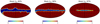Fig. 1. Apodized masks for fsky = 80, 90, and 97% (from left to right).

The power spectra were computed by using the http://www2.iap.fr/users/hivon/software/PolSpice/ estimator, which corrects for multipole-to-multipole coupling and for the mixing of the E- and B- modes due to the sky masking (Chon et al. 2004). We systematically computed the cross-power spectra to ensure we have no bias from any data noise. To compute power spectra at one given frequency, we used the so-called “half-mission” maps (hereafter “HM”). We note that most of the residual instrumental systematic effects evolve with time and are decorrelated between the two half-mission data sets. Throughout the paper, we use 𝒟_ℓ ≡ ℓ(ℓ + 1) 𝒞_ℓ/2π, where 𝒞_ℓ is the original angular power spectrum.

3. Reference models and data simulations

In our analysis of the Planck data, we make use of two reference models of the dust emission and of data simulations, introduced in this section.

3.1. Reference models

The Planck data analysis has shown that the MBB emission law fits well the SED of the dust emission for total intensity (Planck Collaboration XI 2014; Planck Collaboration X 2016) and polarization (Planck Collaboration XI 2020). This provides a convenient and commonly used parametrization of the dust SED:

$$\begin{array}{c}\hfill I_{\mathrm{d}}(\nu )=C_{\nu }^{{\mathrm{UC}}_{\mathrm{K}}}·C_{\nu }^{{\mathrm{CC}}_{\mathrm{d}}}({\beta }_{\mathrm{d}},T_{\mathrm{d}})·{\rho }_{\nu }·{\tau }_{{\nu }_0}{\left(\frac{\nu }{{\nu }_0}\right)}^{{\beta }_{\mathrm{d}}}·B_{\nu }(T_{\mathrm{d}})\end{array}$$(4)

where B_ν(T_d) is the Planck function; T_d, β_d, and τ_ν0 are the dust temperature, spectral index, and optical depth maps at the reference frequency, ν₀, respectively. The MBB emission is expressed in MJy sr⁻¹, whereas the data are given in thermodynamic units. The conversion between the two is accomplished by two factors. The first, $C_{\nu }^{{\text{UC}}_{\text{K}}}$, is a unit conversion from MJy sr⁻¹ to K_CMB for the reference spectral dependence: constant product νI_ν over the bandpass. The second, $C_{\nu }^{{\text{CC}}_{\text{d}}}({\beta }_{\text{d}},T_{\text{d}})$, is the color correction accounting for the difference between the reference spectral dependence and the MBB spectrum. This correction depends on the MBB parameters: β_d and T_d, which are taken to be equal to 1.53 and 19.6 K, respectively (Planck Collaboration XI 2020). The estimated values are presented in Table 1.

In Planck Collaboration III (2020), the polarization efficiencies have been adjusted, within the uncertainties of the ground calibration, in order to match the cosmological parameters derived from the CMB polarization with the ones obtained from CMB temperature (Planck Collaboration III 2020). The factor ρ_ν in Eq. (4) represents this correction to the polarization efficiencies. We use the same values as Planck Collaboration XI (2020), listed in Table 1. The uncertainty on ρ_ν is estimated to be 0.5% at ν = [100, 143, 217] GHz. The correction could not be estimated with the required accuracy at 353 GHz.

We applied Eq. (4) to two sets of MBB parameters derived from Planck component separations methods: i) the GNILC method using maps corrected for anisotropies of the cosmic infrared background and ii) the standard Bayesian analysis framework, implemented in the Commander code (Planck Collaboration X 2016). For GNILC, T_d, β_d, and τ_ν0 have been obtained by fitting a MBB model on the dust total intensity at the Planck frequencies 353, 545, and 857 GHz and IRAS 3000 GHz, while the Commander fit includes all Planck frequencies, together with the nine-year WMAP observations between 23 and 94 GHz (Bennett et al. 2013) and a 408 MHz survey map (Haslam et al. 1982).

To build our reference models, we assume that the dust SED is the same for the total intensity and polarization, an hypothesis supported by the close match between the total intensity and polarization SEDs (Planck Collaboration Int. XXII 2015; Planck Collaboration XI 2020), which we aim to further test in this paper. For GNILC, we also assume that the MBB fitted over the far-IR may be extrapolated to microwave frequencies (Planck Collaboration Int. XVII 2014). Within this framework, the Stokes parameters Q_d(ν) and U_d(ν) at ν = [100, 143, 217] GHz may be computed from the Planck maps at ν₀ = 353 GHz:

$$\begin{array}{cc}\hfill Q_{\mathrm{d}}(\nu )& =\frac{I_{\mathrm{d}}(\nu )}{I_{\mathrm{d}}({\nu }_0)}·(Q_{\mathrm{P}}({\nu }_0)-Q_{\mathrm{P},\mathrm{CMB}}),\hfill \\ \hfill U_{\mathrm{d}}(\nu )& =\frac{I_{\mathrm{d}}(\nu )}{I_{\mathrm{d}}({\nu }_0)}·(U_{\mathrm{P}}({\nu }_0)-U_{\mathrm{P},\mathrm{CMB}}),\hfill \end{array}$$(5)

where Q_P, CMB, and U_P, CMB are CMB Stokes maps from Planck. We use the Planck SMICA CMB maps (Planck Collaboration IV 2020). Our Commander and GNILC models are low-resolution versions of dust models in PySM (Thorne et al. 2017; Zonca et al. 2021), which are commonly used by the CMB community.

3.2. Data simulations

In order to account for the Planck satellite noise, including instrumental systematics and the CMB signal, we computed a set of simulated maps as:

$$\begin{array}{cc}\hfill Q_{\mathrm{sim}}^{\prime }(\nu )& =Q_{\mathrm{d}}(\nu )+Q_{\mathrm{noise}+\mathrm{syst}}(\nu )+Q_{\mathrm{CMB},}\hfill \\ \hfill U_{\mathrm{sim}}^{\prime }(\nu )& =U_{\mathrm{d}}(\nu )+U_{\mathrm{noise}+\mathrm{syst}}(\nu )+U_{\mathrm{CMB}},\hfill \end{array}$$(6)

where [Q_{noise + syst}, U_{noise + syst}] are the 200 SRoll2 simulations to which we subtract the Planck sky model that contain synchrotron, dust, and CMB in order to isolate Planck noise and systematics, (see Delouis et al. 2019, for more details). In addition, [Q_CMB, U_CMB] are 200 independent realizations of the CMB computed from the theoretical power spectra of the best-fit ΛCDM model to the Planck data² (Planck Collaboration VI 2020), with the r parameter equal to 0. Thus, Eq. (6) yields 200 realizations of the reference model maps.

In Fig. 2, we present one realization of the Commander $Q{\prime }_{\mathrm{sim}}$ and $U{\prime }_{\mathrm{sim}}$ maps at 100, 143, and 217 GHz. In Fig. 3, the power spectra of the dust model Commander, the synchrotron template at the two lowest frequencies, the CMB, and a simulation of the SRoll2 noise plus systematics are compared. The mean values ⟨𝒟_ℓ⟩_{ℓ = [4, 32]} for EE (diamonds) and BB (squares) spectra are plotted versus frequency for the three values of f_sky.

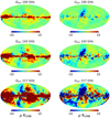Fig. 2. $Q{\prime }_{\mathrm{sim}}$ and $U{\prime }_{\mathrm{sim}}$ reference maps for 100 GHz (top), 143 GHz (middle), and 217 GHz (bottom) as obtained for the Commander reference model.

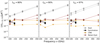Fig. 3. Amplitudes, averaged for 4 < ℓ < 32, of the 𝒟ℓEE (diamond) and BB (square) power spectra versus frequency. Each plot presents the spectra of the Commander dust model (gray), our synchrotron estimate at 100 and 143 GHz (black), the CMB (orange), and the SRoll2 noise plus systematics (light brown). The three plots from left to right correspond to fsky = 80, 90, and 97%.

4. Dust mean SED in polarization

In this section, we derive the mean SED of dust polarization. We use Planck polarization maps at 100, 143, 217, and 353 GHz. The SED values are normalized to the reference frequency, ν₀ = 353 GHz.

We follow earlier studies (Planck Collaboration Int. XXX 2016; Planck Collaboration XI 2020) using cross power spectra to determine the dust mean polarized SED for Planck data γ_P(ν), the reference models γ_d(ν), and the simulations γ_sim(ν) normalized to ν₀ as:

$$\begin{array}{cc}& {\gamma }_{\mathrm{P}}^{\mathrm{XX}}(\nu )={\rho }_{\nu }{\langle \frac{{\mathcal{D}}_{\ell }^{\mathrm{XX}}(\nu \times {\nu }_0)-{\mathcal{D}}_{\ell ,\mathrm{CMB}}^{\mathrm{XX}}}{{\mathcal{D}}_{\ell }^{\mathrm{XX}}({\nu }_0\times {\nu }_0)-{\mathcal{D}}_{\ell ,\mathrm{CMB}}^{\mathrm{XX}}}\rangle }_{{\ell }_{\min },{\ell }_{\max }},\hfill \\ \hfill & {\gamma }_{\mathrm{d}}^{\mathrm{XX}}(\nu )={\langle \frac{{\mathcal{D}}_{\ell ,\mathrm{d}}^{\mathrm{XX}}(\nu \times {\nu }_0)}{{\mathcal{D}}_{\ell ,\mathrm{d}}^{\mathrm{XX}}({\nu }_0\times {\nu }_0)}\rangle }_{{\ell }_{\min },{\ell }_{\max }}\hfill \\ \hfill & {\gamma }_{\mathrm{sim}}^{\mathrm{XX}}(\nu )={\rho }_{\nu }{\langle \frac{{\mathcal{D}}_{\ell ,\mathrm{sim}}^{\mathrm{XX}}(\nu \times {\nu }_0)-{\mathcal{D}}_{\ell ,\mathrm{CMB}}^{\mathrm{XX}}}{{\mathcal{D}}_{\ell ,\mathrm{sim}}^{\mathrm{XX}}({\nu }_0\times {\nu }_0)-{\mathcal{D}}_{\ell ,\mathrm{CMB}}^{\mathrm{XX}}}\rangle }_{{\ell }_{\min },{\ell }_{\max }},\hfill \end{array}$$(7)

where

$$\begin{array}{cc}& {{\mathcal{D}}_{\ell }}^{\mathrm{XX}}(\nu \times {\nu }_0)=[{Q_{\mathrm{P}}^{\prime }}^{\mathrm{HM}1}(\nu ),{U_{\mathrm{P}}^{\prime }}^{\mathrm{HM}1}(\nu )]\times [{Q_{\mathrm{P}}^{\prime }}^{\mathrm{HM}2}({\nu }_0),{U_{\mathrm{P}}^{\prime }}^{\mathrm{HM}2}({\nu }_0)],\hfill \\ \hfill & {{\mathcal{D}}_{\ell ,\mathrm{d}}}^{\mathrm{XX}}(\nu \times {\nu }_0)=[{Q_{\mathrm{d}}}^{\mathrm{HM}1}(\nu ),{U_{\mathrm{d}}}^{\mathrm{HM}1}(\nu )]\times [{Q_{\mathrm{d}}}^{\mathrm{HM}2}({\nu }_0),{U_{\mathrm{d}}}^{\mathrm{HM}2}({\nu }_0)],\hfill \\ \hfill & {{\mathcal{D}}_{\ell ,\mathrm{sim}}}^{\mathrm{XX}}(\nu \times {\nu }_0)=[Q_{\mathrm{sim}}^{\prime \mathrm{HM}1}(\nu ),U_{\mathrm{sim}}^{\prime \mathrm{HM}1}(\nu )]\times [Q_{\mathrm{sim}}^{\prime \mathrm{HM}2}({\nu }_0),U_{\mathrm{sim}}^{\prime \mathrm{HM}2}({\nu }_0)],\hfill \end{array}$$(8)

and ${\mathcal{D}}_{\ell ,\mathrm{CMB}}^{\mathrm{XX}}$ is the CMB power spectrum for the ΛCDM fiducial Planck model (Planck Collaboration VI 2020) with XX ∈ [EE, BB]. ${\mathcal{D}}_{\ell }^{\mathrm{XX}}({\nu }_0\times {\nu }_0)$ is computed with ν = ν₀ in Eq. (8). The symbol × indicates the cross-power spectrum operator and ⟨⟩ the arithmetic mean over the ℓ−range from ℓ_min = 4 to ℓ_max = 32. We note that in the denominator of the first and third equations of Eq. (7), we omit ρ_ν0 because it is equal to 1. Table 2 lists the SED values γ_P(ν) for the Planck data and γ_d(ν) for the reference models, for both EE and BB and for the three sky areas. The uncertainties σ_γP(ν) are derived from the standard deviation of the 200 Planck simulations. The uncertainty on the polarization efficiencies, ρ_ν, and the synchrotron spectral index, β_s, are propagated through our analysis and their contribution to the total error-bar are added to σ_γP.

The dust SEDs Planckγ_P are presented in Fig. 4. The values are normalized to a MBB SED with β_d = 1.53 and T_d = 19.6 K (Planck Collaboration Int. XVII 2014; Planck Collaboration Int. XXII 2015). We note that the value at 353 GHz is always equals to unity because it is the reference frequency considered for our analysis, see Eq. (7). The color corrections $C_{\nu }^{{\text{CC}}_{\text{d}}}({\beta }_{\text{d}}=1.53$ and T_d = 19.6 K) are those listed in Table 1. The figure shows that the γ_P(ν) values are consistent with the MBB used for normalization within 5%, in agreement with previous results (Planck Collaboration Int. XXII 2015; Planck Collaboration XI 2020). Some of the differences could be due to systematics that plagues PR3 data. We note that subtracting the synchrotron emission primarily affects the value of the EE signal to 100 GHz. Although its level is low, around 2–3%. For the mask at 97%, we observe a significant difference between ${\gamma }_{\mathrm{P}}^{\mathit{EE}}(\nu )$ and ${\gamma }_{\mathrm{P}}^{\mathit{BB}}(\nu )$ that we interpret as variations of the SED within the beam, which do not average in the same way for EE and BB. These variations depend also on the mask and could prove more important when the analysis includes a significant part of the Galactic plane.

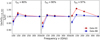Fig. 4. Dust-mean SED γP(ν) normalized by a modified black body function Id(ν) with fixed βd = 1.53 and Td = 19.6 K as given by Planck Collaboration XI (2020) and accounting for color corrections. The EE and BB values are shown in red and blue, respectively. From left to right: Results for fsky = [80, 90, 97]%.

Figure 5 shows the ratio between γ_d for the Commander (top) and GNILC (bottom) models and γ_P. For Commander, we observe a very close match between γ_P(ν) and γ_d(ν) at 143 and 217 GHz for f_sky = 80 and 90% and both EE and BB signals. For GNILC, the match is not as good – we observe in particular a significant difference for f_sky = 80% at 100 and 143 GHz. For f_sky = 97%, we observe a difference between the EE and BB values at 100 GHz. Apart for this latter difference, we observe that γ_d(ν) values are consistent within 5% with the γ_P(ν) values. All the differences between γ_P and γ_d may be due to averaging effects along the line of sight.

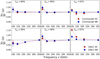Fig. 5. Dust mean SED γd(ν) computed for the reference models: Commander (top row) and GNILC (bottom row). EE and BB values are shown in red and blue, respectively. From left to right: Results for fsky = [80, 90, 97]%. All values are normalized by the γP(ν) values obtained from the data and shown in Fig. 4.

This analysis shows that assuming a reference model based on total intensity data could not completely reproduce the SED observed in polarization data, thus biasing any CMB polarization E-modes and B-modes signals if used as reference for component separation methods. In order to ensure an unbiased detection of the CMB polarization at the precision required from future CMB experiments, we need to address these very small spatial SED variations in the dust polarization emission.

5. Spatial variations in the polarization SED

In this section, we characterize the spatial variations in the dust SED in polarization and quantify the degree of correlation with variations in the dust SED in total intensity.

5.1. Residual maps

To quantify the spatial variations in the dust SED, we compute the differences between the Planck frequency maps at 100, 143, and 217 GHz and the 353 GHz scaled by the mean dust SED γ_P(ν) from Sect. 4, which we approximate as the value of ${\gamma }_{\mathrm{P}}^{\mathit{EE}}(\nu )$ because the dust polarization is dominated by E-modes. Figure 4 shows that ${\gamma }_{\mathrm{P}}^{\mathit{EE}}(\nu )\simeq {\gamma }_{\mathrm{P}}^{\mathit{BB}}(\nu )$ for f_sky = 80%, 90%. A difference between the two coefficients γ_P(ν) is instead detected for f_sky = 97%. This difference indicates a correlation between dust emission properties and the structure of the magnetized interstellar medium. However, we have checked that our approximation also does not significantly impact the results for this f_sky. The three maps, R_Q(ν) and R_U(ν), are then computed as:

$$\begin{array}{cc}\hfill R_{\mathrm{Q}}(\nu )& =Q_{\mathrm{P}}^{\prime }(\nu )-{\gamma }_{\mathrm{P}}(\nu )·Q_{\mathrm{P}}({\nu }_0),\hfill \\ \hfill R_{\mathrm{U}}(\nu )& =U_{\mathrm{P}}^{\prime }(\nu )-{\gamma }_{\mathrm{P}}(\nu )·U_{\mathrm{P}}({\nu }_0),\hfill \end{array}$$(9)

with ν = 100, 143 and 217 GHz, and ν₀ = 353 GHz, which we hereafter refer to as the residual maps and shown in Fig. 6. For comparison, we also compute difference maps for the reference models (see Eq. (10)) and simulations maps replacing γ_P(ν) by γ_d(ν) in Eq. (9):

$$\begin{array}{cc}& R_{{\mathrm{Q}}_{\mathrm{d}}}(\nu )=Q_{\mathrm{d}}(\nu )-{\gamma }_{\mathrm{d}}(\nu )·Q_{\mathrm{d}}({\nu }_0),\hfill \\ \hfill & R_{{\mathrm{U}}_{\mathrm{d}}}(\nu )=U_{\mathrm{d}}(\nu )-{\gamma }_{\mathrm{d}}(\nu )·U_{\mathrm{d}}({\nu }_0),\hfill \\ \hfill & R_{{\mathrm{Q}}_{\mathrm{sim}}^{\prime }}(\nu )=Q_{\mathrm{sim}}^{\prime }(\nu )-{\gamma }_{\mathrm{d}}(\nu )·Q_{\mathrm{sim}}^{\prime }({\nu }_0),\hfill \\ \hfill & R_{{\mathrm{U}}_{\mathrm{sim}}^{\prime }}(\nu )=U_{\mathrm{sim}}^{\prime }(\nu )-{\gamma }_{\mathrm{d}}(\nu )·U_{\mathrm{sim}}^{\prime }({\nu }_0).\hfill \end{array}$$(10)

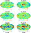Fig. 6. Residual maps RQ (left) and RU (right) at 100, 143, and 217 GHz (shown from top to bottom).

We note that for the purposes of illustration, all the residual maps shown in Figs. 6–8 consider a γ_P(ν) and γ_d(ν) in Eq. (9) computed for f_sky = 90%.

One set of simulation maps [R${}_{\mathrm{Q}{\prime }_{\mathrm{sim}}}$(ν), R${}_{\mathrm{U}{\prime }_{\mathrm{sim}}}$(ν)] for the Commander model is displayed in Fig. 7. The comparison between Figs. 6 and 7 is hampered by Planck data noise but we may notice some common features and some differences. In Fig. 6, we also note differences between frequencies among the R_Q and R_U residual maps, in contrast to what is observed for $R_{\mathrm{Q}{\prime }_{\mathrm{sim}}}$ and $R_{\mathrm{U}{\prime }_{\mathrm{sim}}}$ in Fig. 7. To illustrate that some of the structures are above data noise and uncorrected systematics, in Fig. 8 we present the independent R_Q and R_U residual half-mission HM1 and HM2 maps estimated at 217 GHz. This qualitative examination of the maps suggests that we observe SED variations in the residual R_Q(ν), R_U(ν) maps, which cannot be simply attributed to SED variations in the total intensity, as assumed in the reference models.

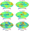Fig. 7. Residual maps for one realization of $R_{Q{\prime }_{\mathrm{sim}}}$ (left) and $R_{U{\prime }_{\mathrm{sim}}}$ (right) obtained for the Commander reference model, at 100, 143, 217 GHz respectively (shown from top to bottom).

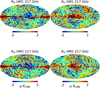Fig. 8. Residual maps RQ (left) and RU (right) at 217 GHz for two data sets HM1 (top), HM2 (bottom), respectively (shown from top to bottom).

5.2. Power-spectra analysis

To characterize the SED variations, we computed power spectra of residual maps and cross-power spectra with the reference models. We computed two cross-power spectra between (i) independent residual maps [$R_{\mathrm{Q}}^{\mathrm{HM}1,\mathrm{HM}2}(\nu )$, $R_{\mathrm{U}}^{\mathrm{HM}1,\mathrm{HM}2}(\nu )$] and (ii) between [$R_{\mathrm{Q}}^{\mathrm{HM}1}(\nu )$, $R_{\mathrm{U}}^{\mathrm{HM}1}(\nu )$] and the reference model residuals [$R_{{\text{Q}}_{\text{d}}}^{\text{HM2}}(\nu )$, $R_{{\text{U}}_{\text{d}}}^{\text{HM2}}(\nu )$]. The 200 simulations are used to assess the impact of data noise plus uncorrected systematics and of the CMB on our analysis.

$$\begin{array}{cc}& {\mathcal{D}}_{\ell ,\mathrm{res}}^{\mathrm{XX}}(\nu )=[R_{\mathrm{Q}}^{\mathrm{HM}1}(\nu ),R_{\mathrm{U}}^{\mathrm{HM}1}(\nu )]\times [R_{\mathrm{Q}}^{\mathrm{HM}2}(\nu ),R_{\mathrm{U}}^{\mathrm{HM}2}(\nu )],\hfill \\ \hfill & {\mathcal{D}}_{\ell ,\mathrm{d},\mathrm{res}}^{\mathrm{XX}}(\nu )=[R_{\mathrm{Q}}^{\mathrm{HM}1}(\nu ),R_{\mathrm{U}}^{\mathrm{HM}1}(\nu )]\times [R_{{\mathrm{Q}}_{\mathrm{d}}}^{\mathrm{HM}2}(\nu ),R_{{\mathrm{U}}_{\mathrm{d}}}^{\mathrm{HM}2}(\nu )],\hfill \\ \hfill & {\mathcal{D}}_{\ell ,\mathrm{sim},\mathrm{res}}^{\mathrm{XX}}(\nu )=[R_{{\mathrm{Q}}_{\mathrm{sim}}^{\prime }}^{\mathrm{HM}1}(\nu ),R_{{\mathrm{U}}_{\mathrm{sim}}^{\prime }}^{\mathrm{HM}1}(\nu )]\times [R_{{\mathrm{Q}}_{\mathrm{sim}}^{\prime }}^{\mathrm{HM}2}(\nu ),R_{{\mathrm{U}}_{\mathrm{sim}}^{\prime }}^{\mathrm{HM}2}(\nu )],\hfill \end{array}$$(11)

where XX ∈ [EE, BB]. Figure 9 shows both sets of cross power spectra for EE (red) and BB (blue) at 100, 143, and 217 GHz for f_sky = 90%. The data points over the ℓ-range 4–32 are compared with the 1σ and 2σ dispersion (dark and light gray shades) obtained with the 200 simulations, including noise and CMB anisotropies (see Sect. 3.2). In all plots, individual data points have a low S/N and it is necessary to average them to quantify mean amplitudes and their frequency dependence.

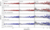Fig. 9. Cross-power spectra correlation ${\mathcal{D}}_{\ell }^{\mathrm{XX}}(\nu )$ and ${\mathcal{D}}_{\ell ,\mathrm{d}}^{\mathrm{XX}}(\nu ),$ indicated as HM1 × HM2 and HM1 × Ref model HM2, respectively, in the labels. Results for fsky = 90% and the Commander reference model are shown. First two rows show the ${\mathcal{D}}_{\ell }^{\mathit{EE}}$ and the last two the ${\mathcal{D}}_{\ell }^{\mathit{BB}}$ cross power spectra, respectively (from top to bottom). Results at 100, 143, and 217 GHz are shown from left to right. The dark and light gray shades represent the 1σ and 2σ standard deviation computed from the data simulations.

The averaged cross power spectra values are computed as:

$$\begin{array}{cc}& A_{\mathrm{res}}(\nu )={\langle {\mathcal{D}}_{\ell ,\mathrm{res}}^{\mathrm{XX}}(\nu )-{(1-{\gamma }_{\mathrm{P}}(\nu ))}^2·{\mathcal{D}}_{\ell ,\mathrm{CMB}}^{\mathrm{XX}}\rangle }_{{\ell }_{\min },{\ell }_{\max }},\hfill \\ \hfill & A_{\mathrm{res},\mathrm{d}}(\nu )={\langle {\mathcal{D}}_{\ell ,\mathrm{d},res}^{\mathrm{XX}}(\nu )\rangle }_{{\ell }_{\min },{\ell }_{\max }},\hfill \\ \hfill & A_{\mathrm{res},\mathrm{sim}}(\nu )={\langle {\mathcal{D}}_{\ell ,\mathrm{res},sim}^{\mathrm{XX}}(\nu )-{(1-{\gamma }_{\mathrm{P}}(\nu ))}^2·{\mathcal{D}}_{\ell ,\mathrm{CMB}}^{\mathrm{XX}}\rangle }_{{\ell }_{\min },{\ell }_{\max }},\hfill \end{array}$$(12)

with XX ∈ [EE, BB]. Notice that the CMB has been partially subtracted in Eqs. (9) and (10). The remaining contribution is accounted for by the term ${(1-{\gamma }_{\mathrm{P}}(\nu ))}^2·{\mathcal{D}}_{\ell ,\mathrm{CMB}}^{\mathrm{XX}}$. In Fig. 10, we plot the amplitudes A_res(ν) normalized by the mean polarized intensity at reference frequency over each sky area defined as:

$$\begin{array}{c}\hfill P_{{\nu }_0}=\sqrt{|Q_{HM1}·Q_{HM2}+U_{HM1}·U_{HM2}|},\end{array}$$(13)

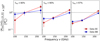Fig. 10. Amplitudes Ares(ν) for EE (red) and BB (blue), respectively. These values are averages over the ℓ-range 4–32 and normalized by the mean of $P_{{\nu }_0}^2$. Results for fsky = [80, 90, 97]% are shown (from left to right).

where HM1 and HM2 refer to the two half-mission maps. We checked that the bias on this estimator of the polarized intensity is negligible at 353 GHz for N_side = 32. This normalization allows us to compare the results for the three different masks. Absolute values of the residuals may be obtained by scaling the figure data points by $\langle P_{{\nu }_0}^2\rangle =[2453.6,5950.5,13814.3]{\text{K}}_{\text{CMB}}$ for f_sky = 80%, 90%, and 97% respectively. We discuss the frequency dependence later, here we focus on the comparison with the models. Figure 11 shows the dust models residuals A_res, d(ν) normalized by A_res(ν). The mean amplitudes A_res, sim(ν) are also computed for each of the 200 simulations and their dispersion provides the error bars. For the 80 and 90% masks, the A_res(ν) are larger by a factor of about ten larger than A_res, d(ν). For these, uncertainties associated with the chance correlation between the CMB and the dust residuals may thus be somewhat underestimated. For the 97% mask, this difference is smaller. At 143 and 217 GHz, the amplitudes even coincide for the GNILC model. These results show that the reference model only accounts for a minor fraction of the total polarization SED variations in the 80 and 90% masks but a much more significant one for the brighter dust emission in the Galactic plane. Furthermore, Fig. 10 highlights the significant variation of BB residuals at 100 GHz toward higher galactic latitudes. Although both the EE and BB variations are very small, in the case of f_sky = 80%, we have $A_{\mathrm{res}}^{\mathit{BB}}$ representing 0.4% of the total amplitude with regard to the 0.1% detected for $A_{\mathrm{res}}^{\mathit{EE}}$. This feature does not match the residuals extrapolated from the models considered (see Fig. 11 for comparison).

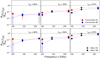Fig. 11. Residual amplitudes Ares, d(ν) obtained for the reference models Commander (top) and GNILC (bottom). Red and blue colors represent the EE and BB results, respectively. These values are estimated by averaging between ℓ-range 4–32 and normalizing to the amplitudes of the residuals obtained from the Planck data Ares(ν). See Eq. (12) for details. Results for fsky = [80, 90, 97]% are shown from left to right. The absolute value of BB negative results found at 100 GHz for fsky = 80% is shown in gray.

To give a more quantitative estimate, we translate the amplitude, A_res(ν), in terms of an effective dispersion of the dust spectral index, σ_β, using the following formula based on a first-order expansion of the MBB emission law in Mangilli et al. (2021):

$$\begin{array}{c}\hfill {\sigma }_{\beta }(\nu )={(A_{\mathrm{res}}^{\mathit{EE}}(\nu )+A_{\mathrm{res}}^{\mathit{BB}}(\nu ))}^{0.5}·{({\gamma }_{\mathrm{P}}(\nu )·P_{{\nu }_0}·|ln\left(\frac{\nu }{{\nu }_0}\right)|)}^{-1}.\end{array}$$(14)

The values of σ_β are listed in Table 3 for the three sky areas and frequencies. These numbers (of about 0.1) must be treated as an estimate of the variance of residuals in terms of pure variation of β. These results are consistent with previous studies at low latitude (Planck Collaboration Int. XLVIII 2016).

6. Residuals from polarization angles

In this section, we quantify the variations in the dust polarization angles as a function of frequency. To do this we introduce the following maps:

$$\begin{array}{cc}\hfill \stackrel{\sim }{Q}(\nu )& ={\gamma }_{\mathrm{P}}(\nu )·P({\nu }_0)\times cos(2\psi (\nu )),\hfill \\ \hfill \stackrel{\sim }{U}(\nu )& ={\gamma }_{\mathrm{P}}(\nu )·P({\nu }_0)\times sin(2\psi (\nu )),\hfill \end{array}$$(15)

where P(ν₀) is the polarized intensity as estimated in Eq. (13), and $\psi (\nu )=\frac{1}{2}arctan\left(\frac{U}{Q}\right)$ is the polarization angle. To assess the contribution of variations in terms of ψ to the total A_res(ν) values, we also computed residual maps for $\stackrel{\sim }{Q}(\nu )$ and $\stackrel{\sim }{U}(\nu )$ as:

$$\begin{array}{cc}\hfill {\stackrel{\sim }{R}}_{\mathrm{Q}}(\nu )& =\stackrel{\sim }{Q}(\nu )-{\gamma }_{\mathrm{P}}(\nu )·\stackrel{\sim }{Q}({\nu }_0),\hfill \\ \hfill {\stackrel{\sim }{R}}_{\mathrm{U}}(\nu )& =\stackrel{\sim }{U}(\nu )-{\gamma }_{\mathrm{P}}(\nu )·\stackrel{\sim }{U}({\nu }_0).\hfill \end{array}$$(16)

The power spectra analysis is performed with these residual maps as described in the previous section:

$$\begin{array}{cc}& {\stackrel{\sim }{\mathcal{D}}}_{\ell ,\mathrm{res}}^{\mathrm{XX}}(\nu )=[{\stackrel{\sim }{R}}_{\mathrm{Q}}^{\mathrm{HM}1}(\nu ),{\stackrel{\sim }{R}}_{\mathrm{U}}^{\mathrm{HM}1}(\nu )]\times [{\stackrel{\sim }{R}}_{\mathrm{Q}}^{\mathrm{HM}2}(\nu ),{\stackrel{\sim }{R}}_{\mathrm{U}}^{\mathrm{HM}2}(\nu )],\hfill \\ \hfill & {\stackrel{\sim }{\mathcal{D}}}_{\ell ,\mathrm{sim},\mathrm{res}}^{\mathrm{XX}}(\nu )=[{\stackrel{\sim }{R}}_{{\mathrm{Q}}_{\mathrm{sim}}^{\prime }}^{\mathrm{HM}1}(\nu ),{\stackrel{\sim }{R}}_{{\mathrm{U}}_{\mathrm{sim}}^{\prime }}^{\mathrm{HM}1}(\nu )]\times [{\stackrel{\sim }{R}}_{{\mathrm{Q}}_{\mathrm{sim}}^{\prime }}^{\mathrm{HM}2}(\nu ),{\stackrel{\sim }{R}}_{{\mathrm{U}}_{\mathrm{sim}}^{\prime }}^{\mathrm{HM}2}(\nu )].\hfill \end{array}$$(17)

And then the averaged amplitudes are defined as:

$$\begin{array}{c}\hfill {\stackrel{\sim }{A}}_{\mathrm{res}}(\nu )={\langle {\stackrel{\sim }{\mathcal{D}}}_{\ell ,\mathrm{res}}^{\mathrm{XX}}(\nu )-{\langle {\stackrel{\sim }{\mathcal{D}}}_{\ell ,\mathrm{sim},res}^{\mathrm{XX}}(\nu )\rangle }_{\mathrm{sim}}\rangle }_{{\ell }_{\min },{\ell }_{\max }},\end{array}$$(18)

where the second term is used for the CMB and residual noise and systematics debiasing. As in Sect. 5.2 for A_res, the uncertainties on ${\stackrel{\sim }{A}}_{\mathrm{res}}$ are derived from the dispersion of the values obtained for the simulations.

Figure 12 compares the ${\stackrel{\sim }{A}}_{\mathrm{res}}(\nu )$ values to A_res(ν). We find that variations of the polarization angle contribute significantly to the total polarization residuals. The differences observed with f_sky may result from the integration along the line of sight or from the limit of our debiasing method (or both). Indeed, for decreasing Galactic latitudes, the line of sight crosses an increasing number of coherent turbulent cells and the impact of the magnetic field structure on observed polarization angles may average out.

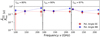Fig. 12. Amplitudes of the residuals ${\stackrel{\sim }{A}}_{\mathrm{res}}(\nu )$ obtained by isolating the effect of the polarization angle variation are shown for EE in red and BB in blue (see Eq. (18)). These values are normalized to the residual amplitudes obtained from the Planck data analysis Ares(ν). Values for fsky = 80, 90, and 97 % are shown from left to right.

To express the amplitude, ${\stackrel{\sim }{A}}_{\mathrm{res}}(\nu ),$ in terms of an effective angle variation, δ_ψ, we assume that the residuals results from a systematic angle change over the full sky area. This calculation is solely indicative because we do not believe that this is a valid assumption. Using equations detailed in Abitbol et al. (2016), we obtain:

$$\begin{array}{c}\hfill sin{\delta }_{\psi }(\nu )=0.5{({\stackrel{\sim }{A}}_{\mathrm{res}}^{\mathit{EE}}(\nu )+{\stackrel{\sim }{A}}_{\mathrm{res}}^{\mathit{BB}}(\nu ))}^{0.5}{\gamma }_{\mathrm{P}}^{-1}(\nu ){(⟨P_{{\nu }_0}^2⟩)}^{-0.5}.\end{array}$$(19)

The values of δ_ψ are listed in Table 3 for three sky areas and frequencies. These values are small but still larger than the 1° uncertainty on the ground calibration of the Planck absolute polarization angle (Rosset et al. 2010) at both 100 and 143 GHz. The analysis of the Planck data confirms this upper limit of 1° (see Fig. 20 in Delouis et al. 2019).

7. Frequency dependence

In this section, we discuss the frequency dependence of the amplitudes of the residuals power spectra plotted in Fig. 10. We follow earlier studies (Chluba et al. 2017; Désert 2022) using a Taylor expansion of the MBB emission law to model the residuals. The moment expansion has been applied to dust power spectra in total intensity by Mangilli et al. (2021) and to dust B-modes power spectra considered as an intensity by Azzoni et al. (2021) and Vacher et al. (2022b). Within this framework, the power spectra of the residual maps are modeled using the first-order expansion as:

$$\begin{array}{cc}\hfill {\mathcal{D}}_{\ell }(\nu )& ={\gamma }_{\mathrm{P}}{(\nu )}^2·\{\hfill \\ \hfill 1\mathrm{st}\text{order}\beta & \{\begin{array}{c}+{\mathcal{D}}_{\ell }^{{\omega }_1^{\beta }\times {\omega }_1^{\beta }}ln{\left(\frac{\nu }{{\nu }_0}\right)}^2,\hfill \end{array}\hfill \\ \hfill 1\mathrm{st}\text{order}T& \{\begin{array}{c}+{\mathcal{D}}_{\ell }^{{\omega }_1^T\times {\omega }_1^T}{({\mathrm{\Theta }}_{\nu }(T_{\mathrm{d}})-{\mathrm{\Theta }}_{{\nu }_0}(T_{\mathrm{d}}))}^2,\hfill \end{array}\hfill \\ \hfill 1\mathrm{st}\text{order}T\mathrm{x}\beta & \{\begin{array}{c}+2{\mathcal{D}}_{\ell }^{{\omega }_1^{\beta }\times {\omega }_1^T}ln\left(\frac{\nu }{{\nu }_0}\right)·({\mathrm{\Theta }}_{\nu }(T_{\mathrm{d}})-{\mathrm{\Theta }}_{{\nu }_0}(T_{\mathrm{d}}))\}.\hfill \end{array}\hfill \end{array}$$(20)

Here, ${\mathcal{D}}_{\mathcal{l}}^{\text{a}\times \text{b}}$ represents three moment coefficients introduced by Mangilli et al. (2021) and Vacher et al. (2022b), which are associated with spatial variations of the dust spectral index and temperature and correlated variations of these two MBB parameters. The Θ_ν(T_d) function is the derivative of the logarithm of the black-body spectrum with respect to temperature T_d:

$$\begin{array}{c}\hfill {\mathrm{\Theta }}_{\nu }(T_{\mathrm{d}})=\frac{x}{T_{\mathrm{d}}}\frac{e^x}{e^x-1},\end{array}$$(21)

where $x=\frac{h\nu }{k_{\mathrm{B}}{T}_{\mathrm{d}}}$. The temperature, T_d, is the one used to normalize γ_P(ν) in Fig. 4.

Ichiki et al. (2019) – and even more extensively Vacher et al. (2023) – have extended the moment expansion to polarization to model the frequency dependence of Stokes Q and U maps. In the formalism introduced by Vacher et al. (2023), the moments are spin-2 objects that characterize the frequency dependence of both polarized intensity and polarization angle. This formalism has not yet been applied to EE and BB power spectra. Qualitatively, we would expect that variations of polarization angles induce an exchange of power between E- and B-modes that is not symmetric due to the E-B asymmetry of dust polarization. The frequency dependence of EE and BB power spectra of residuals maps are thus coupled – but not necessarily identical.

In Fig. 13, we present fits of the $A_{\mathrm{res}}^{\mathit{EE}}(\nu )$ with the three terms in Eq. (20), which we refer to as f₁, f₂ and f₃ for β, T and Txβ, respectively. Over the frequency range of our data analysis from 100 to 217 GHz, these three functions differ only slightly. The f₁ function provides the best fit, especially for f_sky = 97%, but the fits do not allow us to disentangle the contributions from variations of β_d, T_d and their correlation to the power spectra of the residual maps.

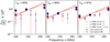Fig. 13. Residual amplitudes Ares(ν), (dark markers) EE (red) and BB (blue) for fsky = [80, 90, 97]%, are shown from left to right. A fit to the data EE accounting for the three components of the moment expansion modeling separately, is described in Eq. (20) and is shown as a dashed line. A cross-power spectra correlation between pair of frequencies: 100 × 143, 100 × 217 and 143 × 217 is shown in smaller and lightened markers.

It is satisfactory to find that the moments’ expansion to the first order provides a good model for the EE power-spectra of residual maps. This result suggests that the residuals follow mainly from variations of dust spectral parameters. However, we can see in the figure that the fits would not be as good for the BB amplitudes, in particular for f_sky = 80%, where the amplitudes do not increase with increasing frequency.

Figure 13 includes amplitudes derived from the 100 × 143, 100 × 217, and 143 × 217 cross-spectra that are plotted with smaller symbols. These data points were not used in the fit because their values depend on frequency decorrelation. We do find that the residual maps at the three frequencies are not fully correlated. The 143 × 217 (and to a lesser extent the 100 × 217) amplitudes lie under the model fit. Part of this mismatch could result from a miscalibration of the absolute polarization angle at 217 GHz. To investigate this possibility, we performed the following test. We rotated the reference frame of the $Q{\prime }_{\mathrm{P}}$, and $U{\prime }_{\mathrm{P}}$ maps at 217 GHz by an angle ψ = ±1°, which is an upper limit based on the Planck polarization absolute angle uncertainty (Delouis et al. 2019). We repeated our analysis with these rotated Stokes maps at 217 GHz for both the Planck data and the simulations to correct for the impact of the rotation on the CMB signal. We found that the amplitudes of 100 × 217 and 143 × 217 do not change in any marked way for either EE and BB, nor for the three masks considered. We conclude from this test that the mismatch between the spectral model and the cross-spectra amplitudes cannot be explained by a miscalibration of the polarization angle in the Planck 217 GHz data.

8. Conclusions

Power spectra of the Planck data were used to characterize spatial variations of the polarized dust SED. We improved the sensitivity of previous studies by using the newly released SRoll2 maps and extending the analysis to regions near the Galactic plane. Our analysis focuses on the lowest multipoles between ℓ = 4 and 32, and three sky areas with f_sky =  80%, 90%, and 97%. Maps of MBB parameters from the Commander and GNILC component separation methods applied to the Planck total intensity data are used as reference models. The main results of our analysis are as follows.

• We confirm earlier studies finding that the mean SED for dust polarization from 100 to 353 GHz is very close to that for the total intensity, as well as to a MBB spectrum with a spectral index of β_d = 1.53 for an assumed dust temperature of T_d = 19.6 K.

• The mean SED and the 353 GHz Q and U maps are used to compute residual maps at 100, 143, and 217 GHz, which quantify spatial variations of the dust polarization SED. Residuals are detected at the three frequencies for the three sky areas. The EE and BB spectra of the residual maps are of comparable amplitude. They do not reproduce the E − B asymmetry that has been observed for the total dust power.

• The residual maps are correlated with the reference Commander and GNILC models, but this correlation accounts for only a fraction of the residuals amplitude. Furthermore, we find that this fraction decreases toward high Galactic latitudes (i.e., for a decreasing f_sky). This result shows that models based on total intensity data are underestimating the complexity of dust polarized CMB foreground. Possibly, future developments of Commander and GNILC models, also accounting for the latest releases of the Planck data, could improve the comparison with polarized data.

• To gain insights into the origin of SED variations, we quantify the variations in the polarization angle. For f_sky  =  80% and 90%, we find that the contribution of polarization angles to the residuals is dominant, in particular for the BB signal. These results emphasize the importance of considering the geometrical properties of Galactic polarization in component separation.

• The frequency dependence of the EE and BB residual amplitudes yields further insights. We find that the moments’ expansion to the first order of the MBB spectrum provides a good fit to the EE amplitudes. This result suggests that the residuals follow mainly from variations of dust spectral parameters (temperature and spectral index). However, this conclusion is challenged by the BB results, particularly for f_sky = 80%, and by cross-spectra that show that the residuals maps at the three frequencies are not fully correlated. Further work (e.g., Vacher et al. 2022a) is needed to model theoretically the impact of polarization angle variations on EE and BB power spectra of residual maps, which we expect to depend on the correlation between the dust emission properties and the structure of the magnetized interstellar medium.

Our analysis of Planck data brings out significant differences between the dust polarization EE and BB SEDs, and with respect to total intensity, setting new requirements for simulations of the dust polarized foreground and component separation methods. A significant refinement to dust modeling is necessary to ensure an unbiased detection of CMB primordial B-modes at the precision required by future CMB experiments.

Acknowledgments

A.R. acknowledges financial support from the French space agency (Centre National d’Etudes Spatiales, CNES) and the Italian Ministry of University and Research - Project Proposal CIR01_00010. F.B. acknowledges support from the Agence Nationale de la Recherche (project BxB: ANR-17-CE31-0022) and CNES. The authors would like to thank the anonymous referee for a thorough reading of the article and for all suggestions and comments that significantly improved the understanding of the text.

References

All Tables

All Figures

	Fig. 1. Apodized masks for fsky = 80, 90, and 97% (from left to right).
In the text

	Fig. 2. $Q{\prime }_{\mathrm{sim}}$ and $U{\prime }_{\mathrm{sim}}$ reference maps for 100 GHz (top), 143 GHz (middle), and 217 GHz (bottom) as obtained for the Commander reference model.
In the text

	Fig. 3. Amplitudes, averaged for 4 < ℓ < 32, of the 𝒟ℓEE (diamond) and BB (square) power spectra versus frequency. Each plot presents the spectra of the Commander dust model (gray), our synchrotron estimate at 100 and 143 GHz (black), the CMB (orange), and the SRoll2 noise plus systematics (light brown). The three plots from left to right correspond to fsky = 80, 90, and 97%.
In the text

	Fig. 4. Dust-mean SED γP(ν) normalized by a modified black body function Id(ν) with fixed βd = 1.53 and Td = 19.6 K as given by Planck Collaboration XI (2020) and accounting for color corrections. The EE and BB values are shown in red and blue, respectively. From left to right: Results for fsky = [80, 90, 97]%.
In the text

	Fig. 5. Dust mean SED γd(ν) computed for the reference models: Commander (top row) and GNILC (bottom row). EE and BB values are shown in red and blue, respectively. From left to right: Results for fsky = [80, 90, 97]%. All values are normalized by the γP(ν) values obtained from the data and shown in Fig. 4.
In the text

	Fig. 6. Residual maps RQ (left) and RU (right) at 100, 143, and 217 GHz (shown from top to bottom).
In the text

	Fig. 7. Residual maps for one realization of $R_{Q{\prime }_{\mathrm{sim}}}$ (left) and $R_{U{\prime }_{\mathrm{sim}}}$ (right) obtained for the Commander reference model, at 100, 143, 217 GHz respectively (shown from top to bottom).
In the text

	Fig. 8. Residual maps RQ (left) and RU (right) at 217 GHz for two data sets HM1 (top), HM2 (bottom), respectively (shown from top to bottom).
In the text

Fig. 9. Cross-power spectra correlation ${\mathcal{D}}_{\ell }^{\mathrm{XX}}(\nu )$ and ${\mathcal{D}}_{\ell ,\mathrm{d}}^{\mathrm{XX}}(\nu ),$ indicated as HM1 × HM2 and HM1 × Ref model HM2, respectively, in the labels. Results for fsky = 90% and the Commander reference model are shown. First two rows show the ${\mathcal{D}}_{\ell }^{\mathit{EE}}$ and the last two the ${\mathcal{D}}_{\ell }^{\mathit{BB}}$ cross power spectra, respectively (from top to bottom). Results at 100, 143, and 217 GHz are shown from left to right. The dark and light gray shades represent the 1σ and 2σ standard deviation computed from the data simulations.

In the text

	Fig. 10. Amplitudes Ares(ν) for EE (red) and BB (blue), respectively. These values are averages over the ℓ-range 4–32 and normalized by the mean of $P_{{\nu }_0}^2$. Results for fsky = [80, 90, 97]% are shown (from left to right).
In the text

Fig. 11. Residual amplitudes Ares, d(ν) obtained for the reference models Commander (top) and GNILC (bottom). Red and blue colors represent the EE and BB results, respectively. These values are estimated by averaging between ℓ-range 4–32 and normalizing to the amplitudes of the residuals obtained from the Planck data Ares(ν). See Eq. (12) for details. Results for fsky = [80, 90, 97]% are shown from left to right. The absolute value of BB negative results found at 100 GHz for fsky = 80% is shown in gray.

In the text

	Fig. 12. Amplitudes of the residuals ${\stackrel{\sim }{A}}_{\mathrm{res}}(\nu )$ obtained by isolating the effect of the polarization angle variation are shown for EE in red and BB in blue (see Eq. (18)). These values are normalized to the residual amplitudes obtained from the Planck data analysis Ares(ν). Values for fsky = 80, 90, and 97 % are shown from left to right.
In the text

Fig. 13. Residual amplitudes Ares(ν), (dark markers) EE (red) and BB (blue) for fsky = [80, 90, 97]%, are shown from left to right. A fit to the data EE accounting for the three components of the moment expansion modeling separately, is described in Eq. (20) and is shown as a dashed line. A cross-power spectra correlation between pair of frequencies: 100 × 143, 100 × 217 and 143 × 217 is shown in smaller and lightened markers.

In the text

References

- Abazajian, K. N., Adshead, P., Ahmed, Z., et al. 2016, ArXiv e-prints [arXiv:1610.02743] [Google Scholar]
- Abitbol, M. H., Hill, J. C., & Johnson, B. R. 2016, MNRAS, 457, 1796 [Google Scholar]
- Ade, P. A. R., Aguirre, J., Ahmed, Z., et al. 2019, JCAP, 2019, 056 [CrossRef] [Google Scholar]
- Ade, P. A. R., Ahmed, Z., Amiri, M., et al. 2022, ApJ, 927, 77 [NASA ADS] [CrossRef] [Google Scholar]
- Ashton, P. C., Ade, P. A. R., Angilè, F. E., et al. 2018, ApJ, 857, 10 [Google Scholar]
- Azzoni, S., Abitbol, M. H., Alonso, D., et al. 2021, JCAP, 2021, 047 [CrossRef] [Google Scholar]
- Benabed, K., Cardoso, J. F., Prunet, S., & Hivon, E. 2009, MNRAS, 400, 219 [NASA ADS] [CrossRef] [Google Scholar]
- Bennett, C. L., Larson, D., Weiland, J. L., et al. 2013, ApJS, 208, 20 [Google Scholar]
- Chluba, J., Hill, J. C., & Abitbol, M. H. 2017, MNRAS, 472, 1195 [NASA ADS] [CrossRef] [Google Scholar]
- Chon, G., Challinor, A., Prunet, S., Hivon, E., & Szapudi, I. 2004, MNRAS, 350, 914 [Google Scholar]
- de la Hoz, E. 2022, ArXiv e-prints [arXiv:2203.04861] [Google Scholar]
- Delouis, J. M., Pagano, L., Mottet, S., Puget, J. L., & Vibert, L. 2019, A&A, 629, A38 [NASA ADS] [CrossRef] [EDP Sciences] [Google Scholar]
- Désert, F.-X. 2022, A&A, 659, A70 [NASA ADS] [CrossRef] [EDP Sciences] [Google Scholar]
- Fixsen, D. J., Bennett, C. L., & Mather, J. C. 1999, ApJ, 526, 207 [Google Scholar]
- Górski, K. M., Hivon, E., Banday, A. J., et al. 2005, ApJ, 622, 759 [Google Scholar]
- Guillet, V., Fanciullo, L., Verstraete, L., et al. 2018, A&A, 610, A16 [NASA ADS] [CrossRef] [EDP Sciences] [Google Scholar]
- Guth, A. H. 1981, Phys. Rev. D, 23, 347 [Google Scholar]
- Haslam, C. G. T., Salter, C. J., Stoffel, H., & Wilson, W. E. 1982, A&AS, 47, 1 [NASA ADS] [Google Scholar]
- Hensley, B. S., & Bull, P. 2018, ApJ, 853, 127 [NASA ADS] [CrossRef] [Google Scholar]
- Hensley, B. S., & Draine, B. T. 2022, ApJ, submitted [arXiv:2208.12365] [Google Scholar]
- Ichiki, K., Kanai, H., Katayama, N., & Komatsu, E. 2019, Prog. Theor. Exp. Phys., 2019, 033E01 [CrossRef] [Google Scholar]
- Kamionkowski, M., & Kovetz, E. D. 2016, ARA&A, 54, 227 [NASA ADS] [CrossRef] [Google Scholar]
- Krachmalnicoff, N., Carretti, E., Baccigalupi, C., et al. 2018, A&A, 618, A166 [NASA ADS] [CrossRef] [EDP Sciences] [Google Scholar]
- Linde, A. 1982, Phys. Lett. B, 116, 335 [NASA ADS] [CrossRef] [Google Scholar]
- LiteBIRD Collaboration (Allys, E., et al.) 2022, ArXiv e-prints [arXiv:2202.02773] [Google Scholar]
- Mangilli, A., Aumont, J., Rotti, A., et al. 2021, A&A, 647, A52 [NASA ADS] [CrossRef] [EDP Sciences] [Google Scholar]
- Martire, F. A., Barreiro, R. B., & Martínez-González, E. 2022, JCAP, 2022, 003 [CrossRef] [Google Scholar]
- Mennella, A., Bersanelli, M., Butler, R. C., et al. 2011, A&A, 536, A3 [NASA ADS] [CrossRef] [EDP Sciences] [Google Scholar]
- Osumi, K., Weiland, J. L., Addison, G. E., & Bennett, C. L. 2021, ApJ, 921, 175 [NASA ADS] [CrossRef] [Google Scholar]
- Pelgrims, V., Clark, S. E., Hensley, B. S., et al. 2021, A&A, 647, A16 [NASA ADS] [CrossRef] [EDP Sciences] [Google Scholar]
- Planck Collaboration IX. 2014, A&A, 571, A9 [NASA ADS] [CrossRef] [EDP Sciences] [Google Scholar]
- Planck Collaboration XI. 2014, A&A, 571, A11 [NASA ADS] [CrossRef] [EDP Sciences] [Google Scholar]
- Planck Collaboration Int. XVII. 2014, A&A, 566, A55 [NASA ADS] [CrossRef] [EDP Sciences] [Google Scholar]
- Planck Collaboration Int. XXII. 2015, A&A, 576, A107 [NASA ADS] [CrossRef] [EDP Sciences] [Google Scholar]
- Planck Collaboration VIII. 2016, A&A, 594, A8 [NASA ADS] [CrossRef] [EDP Sciences] [Google Scholar]
- Planck Collaboration X. 2016, A&A, 594, A10 [NASA ADS] [CrossRef] [EDP Sciences] [Google Scholar]
- Planck Collaboration Int. XXX. 2016, A&A, 586, A133 [NASA ADS] [CrossRef] [EDP Sciences] [Google Scholar]
- Planck Collaboration Int. XLVI. 2016, A&A, 596, A107 [NASA ADS] [CrossRef] [EDP Sciences] [Google Scholar]
- Planck Collaboration Int. XLVIII. 2016, A&A, 596, A109 [NASA ADS] [CrossRef] [EDP Sciences] [Google Scholar]
- Planck Collaboration Int. L. 2017, A&A, 599, A51 [NASA ADS] [CrossRef] [EDP Sciences] [Google Scholar]
- Planck Collaboration III. 2020, A&A, 641, A3 [NASA ADS] [CrossRef] [EDP Sciences] [Google Scholar]
- Planck Collaboration IV. 2020, A&A, 641, A4 [NASA ADS] [CrossRef] [EDP Sciences] [Google Scholar]
- Planck Collaboration V. 2020, A&A, 641, A5 [NASA ADS] [CrossRef] [EDP Sciences] [Google Scholar]
- Planck Collaboration VI. 2020, A&A, 641, A6 [NASA ADS] [CrossRef] [EDP Sciences] [Google Scholar]
- Planck Collaboration XI. 2020, A&A, 641, A11 [NASA ADS] [CrossRef] [EDP Sciences] [Google Scholar]
- Planck HFI Core Team 2011, A&A, 536, A4 [NASA ADS] [CrossRef] [EDP Sciences] [Google Scholar]
- Puglisi, G., Fabbian, G., & Baccigalupi, C. 2017, MNRAS, 469, 2982 [NASA ADS] [CrossRef] [Google Scholar]
- Rosset, C., Tristram, M., Ponthieu, N., et al. 2010, A&A, 520, A13 [NASA ADS] [CrossRef] [EDP Sciences] [Google Scholar]
- Svalheim, T. L., Andersen, K. J., Aurlien, R., et al. 2023, A&A, in press, https://doi.org/10.1051/0004-6361/202243160 [Google Scholar]
- Tassis, K., & Pavlidou, V. 2015, MNRAS, 451, L90 [NASA ADS] [CrossRef] [Google Scholar]
- Thorne, B., Dunkley, J., Alonso, D., & Næss, S. 2017, MNRAS, 469, 2821 [Google Scholar]
- Vacher, L., Aumont, J., Boulanger, F., et al. 2022a, A&A, submitted [arXiv:2210.14768] [NASA ADS] [CrossRef] [EDP Sciences] [Google Scholar]
- Vacher, L., Aumont, J., Montier, L., et al. 2022b, A&A, 660, A111 [NASA ADS] [CrossRef] [EDP Sciences] [Google Scholar]
- Vacher, L., Chluba, J., Aumont, J., Rotti, A., & Montier, L. 2023, A&A, 669, A5 [NASA ADS] [CrossRef] [EDP Sciences] [Google Scholar]
- Weiland, J. L., Addison, G. E., Bennett, C. L., Halpern, M., & Hinshaw, G. 2022, ApJ, 936, 24 [NASA ADS] [CrossRef] [Google Scholar]
- Zonca, A., Thorne, B., Krachmalnicoff, N., & Borrill, J. 2021, J. Open Source Softw., 6, 3783 [NASA ADS] [CrossRef] [Google Scholar]
All Tables
Unit conversions and color corrections, , taken from Planck Collaboration IX (2014).
Dust mean SED values for the Planck polarization data γP(ν) and the reference models γd(ν).
Effective dispersion of the dust spectral index σβ and effective angle variation δψ.