| Issue |
A&A
Volume 669, January 2023
|
|
|---|---|---|
| Article Number | A119 | |
| Number of page(s) | 25 | |
| Section | Galactic structure, stellar clusters and populations | |
| DOI | https://doi.org/10.1051/0004-6361/202244957 | |
| Published online | 20 January 2023 | |
The Gaia-ESO survey: Mapping the shape and evolution of the radial abundance gradients with open clusters
1
INAF – Osservatorio Astrofisico di Arcetri, Largo E. Fermi 5, 50125 Firenze, Italy
e-mail: This email address is being protected from spambots. You need JavaScript enabled to view it.
2
Institute of Theoretical Physics and Astronomy, Vilnius University, Sauletekio av. 3, 10257 Vilnius, Lithuania
3
INAF – Padova Observatory, Vicolo dell’Osservatorio 5, 35122 Padova, Italy
4
INAF – Osservatorio di Astrofisica e Scienza dello Spazio di Bologna, Via Gobetti 93/3, 40129 Bologna, Italy
5
Université Côte d’Azur, Observatoire de la Côte d’Azur, CNRS, Laboratoire Lagrange, 06304 Nice, France
6
Research School of Astronomy and Astrophysics, Australian National University, Canberra, ACT 2611, Australia
7
ARC Centre of Excellence for Astronomy in Three Dimensions (ASTRO-3D), Canberra, ACT 2611, Australia
8
Dipartimento di Fisica, Università degli Studi di Roma Tor Vergata, Via della Ricerca scientifica 1, 00133 Roma, Italy
9
Leibniz-Institut für Astrophysik Potsdam (AIP), An der Sternwarte 16, 14482 Potsdam, Germany
10
Nicolaus Copernicus Astronomical Center, Polish Academy of Sciences, ul. Bartycka 18, 00-716 Warsaw, Poland
11
ESO, Karl Schwarzschild Strasse 2, 85748 Garching, Germany
12
Dipartimento di Fisica e Astronomia, Università degli studi di Bologna, Via Gobetti 93/2, 40129 Bologna, Italy
13
Lund Observatory, Department of Astronomy and Theoretical Physics, Box 43, 221 00 Lund, Sweden
14
Space Science Data Center – agenzia Spaziale Italiana, Via del Politecnico, s.n.c., 00133 Roma, Italy
15
Observational Astrophysics, Department of Physics and Astronomy, Uppsala University, Box 516, 75120 Uppsala, Sweden
16
INAF – Rome Observatory, Via Frascati, 33, Monte Porzio Catone, (RM), Italy
17
Institute of Astronomy, University of Cambridge, Madingley Road, Cambridge CB3 0HA, UK
18
Max Planck Institute for Astronomy, Konigstuhl 17, 69117 Heidelberg, Germany
19
Niels Bohr International Academy, Niels Bohr Institute, University of Copenhagen, Blegdamsvej 17, 2100 Copenhagen, Denmark
Received:
12
September
2022
Accepted:
26
October
2022
Abstract
Context. The spatial distribution of elemental abundances and their time evolution are among the major constraints to disentangling the scenarios of formation and evolution of the Galaxy.
Aims. In this paper we used the sample of open clusters available in the final release of the Gaia-ESO survey to trace the Galactic radial abundance and abundance-to-iron ratio gradients, and their time evolution.
Methods. We selected member stars in 62 open clusters, with ages from 0.1 to about 7 Gyr, located in the Galactic thin disc at galactocentric radii (RGC) from about 6 to 21 kpc. We analysed the shape of the resulting [Fe/H] gradient, the average gradients [El/H] and [El/Fe] combining elements belonging to four different nucleosynthesis channels, and their individual abundance and abundance ratio gradients. We also investigated the time evolution of the gradients dividing open clusters in three age bins.
Results. The [Fe/H] gradient has a slope of −0.054 dex kpc−1. It can be better approximated with a two-slope shape, steeper for RGC ≤ 11.2 kpc and flatter in the outer regions. We saw different behaviours for elements belonging to different channels. For the time evolution of the gradient, we found that the youngest clusters (age < 1 Gyr) in the inner disc have lower metallicity than their older counterparts and that they outline a flatter gradient. We considered some possible explanations, including the effects of gas inflow and migration. We suggest that the most likely one may be related to a bias introduced by the standard spectroscopic analysis producing lower metallicities in the analysis of low-gravity stars.
Conclusions. To delineate the shape of the ‘true’ gradient, we should most likely limit our analysis to stars with low surface gravity log g > 2.5 and microturbulent parameter ξ < 1.8 km s−1. Based on this reduced sample, we can conclude that the gradient has minimally evolved over the time-frame outlined by the open clusters, indicating a slow and stationary formation of the thin disc over the last 3 Gyr. We found a secondary role of cluster migration in shaping the gradient, with a more prominent role of migration for the oldest clusters.
Key words: stars: abundances / stars: evolution / open clusters and associations: general / Galaxy: evolution
© The Authors 2023
 Open Access article, published by EDP Sciences, under the terms of the Creative Commons Attribution License (https://creativecommons.org/licenses/by/4.0), which permits unrestricted use, distribution, and reproduction in any medium, provided the original work is properly cited.
This article is published in open access under the Subscribe-to-Open model. This email address is being protected from spambots. You need JavaScript enabled to view it. to support open access publication.
1. Introduction
Open clusters (OCs) are considered excellent tracers of the chemical properties of the thin-disc stellar populations of our Galaxy, including the spatial distribution of elemental abundances. Since the end of the 1970s, several works have exploited the use of OCs to trace the radial distribution, initially of metallicity and then of individual elements (see e.g. Mayor 1976; Janes 1979; Janes et al. 1988; Friel & Janes 1993; Carraro & Chiosi 1994; Friel 1995; Twarog et al. 1997; Friel et al. 2002). Considered on their own, or appropriately combined with other stellar and nebular Galactic tracers that correspond to different epochs in the evolution of our Galaxy, such as H II regions (e.g. Peimbert et al. 1978; Balser et al. 2011; Esteban et al. 2017; Arellano-Córdova et al. 2020; Méndez-Delgado et al. 2022), young massive O and B stars (e.g. Daflon & Cunha 2004; Rolleston et al. 2000; Bragança et al. 2019), young late-type stars (e.g. Padgett 1996; Cunha et al. 1998; Biazzo et al. 2011), Cepheid variable stars (e.g. Pedicelli et al. 2009; Lemasle et al. 2007, 2008, 2013; Genovali et al. 2014, 2015; Luck 2018; da Silva et al. 2022; Kovtyukh et al. 2022), and planetary nebulae (e.g. Maciel et al. 2003; Perinotto & Morbidelli 2006; Henry et al. 2010; Stanghellini & Haywood 2010, 2018), OCs have broadened our understanding of the processes of thin disc formation and evolution.
The best use of OCs as tracers of chemical evolution is possible when spectroscopic observations at high spectral resolution are available, from which detailed elemental abundances of cluster member stars can be derived. In the past many spectroscopic observations were performed with a single slit or fibre, thus observing one star at a time, as in the Bologna Open Cluster Chemical Evolution (BOCCE) project (Bragaglia 2008; Donati et al. 2012, 2014; Ahumada et al. 2013) and other studies (e.g. Yong et al. 2005, 2012; Casamiquela et al. 2016, 2017, 2019). Subsequently, the employment of new multi-fibre instruments such as Hydra-WIYN (von Hippel & Sarajedini 1998) and the FLAMES instrument on the ESO VLT (Pasquini et al. 2002) made it possible to study many members of the same cluster simultaneously. The exploitation of FLAMES at the VLT favoured the realisation of many large programmes dedicated to the study of open clusters (Randich et al. 2003, 2005, 2006; Randich et al. 2007; Sestito et al. 2003, 2004, 2006; Sestito et al. 2007, 2008a,b). The following years were witness to an enlargement of the sample of OCs with high-resolution spectroscopic observations, providing innovative information on both the inner disc (e.g. Magrini et al. 2010; Reddy et al. 2016; Jacobson et al. 2016; Casamiquela et al. 2019) and the outer disc (e.g. Carraro et al. 2007; Yong et al. 2012). A few years later, the era of large spectroscopic surveys started, also aimed at complementing the subsequent exploitation of the data coming from the Gaia satellite, which was launched in 2013 (Gaia Collaboration 2016b,a, 2018; Gaia Collaboration 2021). Among these the Gaia-ESO survey (Gilmore et al. 2012, 2022; Randich et al. 2013, 2022), the only one performed on a 8 m class telescope, put a specific focus on the Galactic population of OCs; Gaia-ESO targeted OCs over a wide range of ages, distances, masses, and metallicities, observing large unbiased samples of cluster candidates, with a well-defined selection function (Bragaglia et al. 2022; Randich et al. 2022).
Although focused on the Milky Way field, the other two large surveys at medium to high spectral resolution, GALactic Archeology with HERMES (GALAH; De Silva et al. 2015) and Apache Point Observatory Galactic Evolution Experiment (APOGEE; Majewski et al. 2017), also include several clusters in their samples that allowed them to address the issue of the radial distribution of chemical abundances (e.g. Donor et al. 2018, 2020; Spina et al. 2021; Myers et al. 2022). There is also an important contribution from the lower-resolution spectroscopic survey performed by the Large sky Area Multi-Object fiber Spectroscopic Telescope (LAMOST; Zhao et al. 2012), whose data, combined with those from the Gaia mission, helped define the shape of the gradient (e.g. Chen et al. 2009; Zhong et al. 2020; Fu et al. 2022). The contribution of Gaia with its elemental abundances measured from spectra taken with the onboard RVS spectrograph is adding further constraints and has already delineated the Galactic gradient with its DR3 (Gaia Collaboration 2023). Many more clusters will be included in the coming years thanks to instruments dedicated to spectroscopic surveys, such as WEAVE (Dalton et al. 2018) and 4MOST (de Jong et al. 2019). A review of the state of the art of the radial [Fe/H] gradient, obtained combining and homogenising the data of open clusters from the three main high-resolution spectroscopic surveys (Gaia-ESO, APOGEE, and GALAH) is presented in Spina et al. (2022). However, there are numerous questions that are not completely resolved and on which full consensus has not been reached yet, such as whether there is a time evolution of the gradient traced by clusters in different age bins and if the gradient is flattening or steepening with time; whether clusters are affected by migration as much as isolated stars; and, finally, if there is a global relationship between age and metallicity for clusters or whether such a relationship exists only when considering limited intervals in galactocentric distance. In this paper we use the sample of OCs observed by the Gaia-ESO survey (excluding the youngest ones with ages < 100 Myr) to investigate some aspects of the above-mentioned open issues, in particular those related to the abundance gradients, namely the shape of the abundance gradients and their link with the different nucleosynthesis channels; their temporal change with its implication for Galactic chemical evolution, the role of migration, and the possible effects due to spectral analysis; and the impact of the disc warp, with its variation with time, on the shape and evolution of the gradients. The structure of the paper is as follows. In Sect. 2 we describe the abundance analysis and sample selection. In Sect. 3 we analyse the shape of the [Fe/H] and elemental abundance gradients. In Sect. 4 we present the time-evolution of the gradients, and in Sect. 5 we discuss its possible origins. In Sect. 6, we select an unbiased sample of stars to trace the time-evolution of the gradient. Finally, in Sect. 7 we provide our summary and conclusions.
2. Abundance analysis and sample selection
2.1. Elemental abundance determination in the Gaia-ESO UVES spectra
In this work we adopted the final data release of the Gaia-ESO Survey, selecting only the stellar parameters and abundances from the high-resolution UVES spectra (resolving power R = 47 000), covering the spectral range 480.0−680.0 nm. In particular, we considered only the spectra analysed by Working Group 11 (WG 11), which is in charge of the analysis of UVES spectra of FGK stars in the field and clusters. The structure of the Gaia-ESO WGs is described in Gilmore et al. (2022). The data reduction and analysis were performed by the Gaia-ESO consortium, as described in Sacco et al. (2014), Smiljanic et al. (2014), Randich et al. (2022) and Gilmore et al. (2022), among others. The main steps for the analysis of the UVES spectra are as follows: (i) data reduction, including radial and rotational velocity determinations carried out at the Istituto Nazionale di Astrofisica (INAF) for UVES using the FLAMES-UVES ESO public pipeline (Sacco et al. 2014); (ii) spectral analysis with a multi-pipeline strategy, shared within the same WG, among different nodes, and internally homogenised (see Smiljanic et al. 2014; Randich et al. 2022, for details); (iii) homogenisation of the WG results on a common scale, and production of the final database using, as calibrators, benchmark stars, open clusters, and globular clusters (see Pancino et al. 2017; Hourihane et al. 2022, for a description of the strategy and its application). The recommended parameters and abundances are distributed in the IDR6 catalogue, including those used in the present work: atmospheric stellar parameters Teff, log g, [Fe/H], elemental abundances, and radial velocities (RVs). The catalogue is also publicly available in the ESO archive1.
2.2. Elemental abundances
For this work we considered a total of 25 chemical elements, including iron, from different nucleosynthesis processes. We used the following abundances: (i) O, Mg, Si, Ca, Ti, considered representative of the class of the α elements, produced by massive stars (e.g. Woosley & Weaver 1995); (ii) two odd-Z elements, namely Na and Al, which show a similar evolution as the α elements (see Smiljanic et al. 2016, for a description of the main astrophysical sites for the production of these elements); (iii) several iron-peak elements, namely Sc, V, Cr, Mn, Co, Fe, and Ni; (iv) Cu and Zn, which have a more uncertain origin; most Cu production on Galactic scales might be due to the weak s-process acting in massive stars (Romano & Matteucci 2007), and large fractions of Zn at low metallicities may come from hypernovae or pair-instability supernovae (SNe; Kobayashi et al. 2020), while the situation at high metallicities is less clear; and (v) a number of neutron-capture elements, whose availability is unique compared to other large spectroscopic surveys, thanks to the higher resolution and spectral coverage of Gaia-ESO. Among the elements whose origin is dominated by the slow (s) process we used Y, Zr, Ba, La, and Ce, and among those dominated by the rapid (r) process we used Mo, Pr, Nd, and Eu.
2.3. Solar scale normalisation
Most of the stars observed in our sample of OCs are in the giant phase (∼75%); specifically, they are red giant branch or red clump stars. In some of the clusters Gaia-ESO also observed dwarf stars in the main sequence (MS) phase (see Randich et al. 2022; Bragaglia et al. 2022). To produce solar-scaled abundances, we adopted a normalisation procedure based on the abundances of giant and dwarf stars in the open cluster M67 known to have a composition very similar to the solar one (see e.g. Önehag et al. 2011; Liu et al. 2016).
In Table A.1 we show the solar abundances in Gaia-ESO IDR6; the solar abundances of Grevesse et al. (2007), which are the reference for the input model atmospheres and the synthetic spectra in Gaia-ESO; the average abundances of M67; and those for its giant (log g < 3.5) and dwarf (log g ≥ 3.5) member stars (from the Gaia-ESO IDR6). For the membership analysis we refer to Magrini et al. (2021a). The agreement between the solar and average M67 Gaia-ESO abundances and those of Grevesse et al. (2007) is very good, within 1σ for most elements. A slightly worse agreement, within 2σ, is obtained for some elements (O, Al, Ca, Si, Cu, Ce). The differences between abundances in dwarf and giant stars can be attributed both to physical effects, such as stellar diffusion, and to spectral analysis issues (cf. Önehag et al. 2014; Bertelli Motta et al. 2018; Souto et al. 2019). In our analysis we adopted the two sets of abundances to normalise, respectively, the sample of giant and dwarf stars in OCs. This choice has some impact for elements more influenced by changes when measured in dwarfs or giants (Mg, Si, Ca, Na, Al), but also for some of the neutron capture elements (e.g. Zr, La, Ce).
2.4. Open cluster sample
Here we considered the 62 OCs older than 100 Myr, as in Viscasillas Vázquez et al. (2022). Abundances in stars belonging to younger clusters might need a specific analysis (Baratella et al. 2020, 2021; Spina et al. 2021; Zhang et al. 2021a), since they can be affected by magnetic activity and rotation, influencing the determination of the microturbulent parameter, ξ, and, in turn, of the whole set of stellar parameters and abundances. In addition, these clusters represent only the latest instants in the global Galactic chemical evolution, characterised by negligible variations with respect to the total timescale. For these reasons, we did not include them in this work. For the distribution in age and distances of our sample clusters we refer to Viscasillas Vázquez et al. (2022, see their Fig. 1), and for a general description of the open cluster sample in Gaia-ESO to Randich et al. (2022) and Bragaglia et al. (2022).
For each cluster we performed the membership analysis as in Magrini et al. (2021a) and in Viscasillas Vázquez et al. (2022). Specifically, for 41 clusters we used the membership probability provided by Jackson et al. (2022), while for the remaining clusters we adopted the analysis of Magrini et al. (2021a). Both membership analyses are based on three-dimensional kinematics, complementing the RVs from Gaia-ESO with proper motions and parallaxes from GaiaEDR3 (Gaia Collaboration 2021). Since for clusters we rely on the average abundances of all members, it is not necessary to introduce a cutoff on the abundances of each individual member based on the signal-to-noise ratio or the errors on parameters. We only discarded stars with high errors on abundance ≥0.1 dex. In addition, for each cluster we used the interquartile range rule to detect potential outliers that fall outside of the overall abundance pattern.
We provide in Tables A.2–A.6 the global metallicity of each cluster from Randich et al. (2022) together with the galactocentric distances, RGC; the age (Cantat-Gaudin et al. 2020); and the abundance ratios used throughout the paper. For clusters whose [Fe/H] was not available in Randich et al. (2022), we computed the average [Fe/H] using the cluster members adopted in the present work. In Table A.7 we provide the number of member stars used to compute the abundance ratios per cluster and per element.
3. Shape of radial abundance and abundance ratio gradients
The shape of the metallicity gradient is an important observational constraint for defining the timescales of the formation of the Galactic thin disc, the radial variations of the star formation rate, of its efficiency and of the gas infall. Open clusters have been used to track the gradient for many decades (see e.g. Janes 1979), and many papers have highlighted the bimodal nature of the gradient, with a break in abundances at around RGC ∼ 10 − 12 kpc, beyond which the gradient becomes flatter (e.g. Bragaglia et al. 2008; Sestito et al. 2008a; Friel et al. 2010; Pancino et al. 2010; Carrera & Pancino 2011; Yong et al. 2012; Frinchaboy et al. 2013; Reddy et al. 2016; Magrini et al. 2017; Casamiquela et al. 2019; Donor et al. 2020; Zhang et al. 2021b; Netopil et al. 2022; Spina et al. 2022; Myers et al. 2022). There is a general agreement for the existence of a steeper gradient in the inner disc and an extended plateau in the outer regions, although there is no substantial difference in the goodness of the fits done with a single slope compared to those with two slopes.
In Table 1 we present some recent determinations of the slope of the radial [Fe/H] gradient with OCs. The global slope of the gradient in the literature varies from −0.054 to −0.077 dex kpc−1. Samples that contain mainly inner clusters have a steeper slope (see e.g. Carrera et al. 2019; Spina et al. 2021; Myers et al. 2022; Donor et al. 2020; Zhang et al. 2021b), while samples reaching the Galaxy outskirts have flat global gradients (see e.g. Spina et al. 2022; Netopil et al. 2022). The gradient sampled by the Gaia Collaboration (2023) is an exception since it is limited to the regions between RGC ∼ 5 to 12 kpc, but it is quite flat, −0.054 dex kpc−1. In the last row of the table, we put as reference the gradient of the Cepheids, computed with the high-quality sample of Genovali et al. (2014).
Slopes of the [Fe/H] gradient from open cluster samples, from the recent literature.
3.1. Shape of [Fe/H] gradient
In the next sections we discuss our determination of the shape of the [Fe/H] and elemental abundance gradients. We adopted two different approaches to fit the data: a locally weighted linear regression (LOWESS), estimated using a non-parametric regression method that combines multiple regression models in a k-nearest-neighbour-based meta-model, and a classical linear regression model fit with its confidence interval. The former allowed us to follow the behaviour of the data better, while the latter allowed us to compare with linear fits available in the literature, and to compare with our results with the slopes provided in previous works.
In Fig. 1 we show the radial distribution of [Fe/H] as traced by our sample of OCs, with the results of the two fitting procedures. In this figure we plot together clusters of all ages. There is a non-negligible scatter at each RGC related to several aspects that we expand on in the next sections. In the upper panel we present a global fit of the sample over the whole radial range. There is a clear downward trend; the inner clusters reach [Fe/H] values up to about +0.4, and the outer clusters reach [Fe/H] ∼ −0.4. The scatter increases in the transition region, from the steeper inner gradient to the flatter one, by around 10–12 kpc, but it is also quite high in the inner regions. Considering a weighted single-slope fit, the shape of the gradient is
![Mathematical equation: $$ \begin{aligned} \mathrm{[Fe/H]}= -0.054(\pm 0.004)\times R_{\rm GC}+0.474(\pm 0.045) \end{aligned} $$](/articles/aa/full_html/2023/01/aa44957-22/aa44957-22-eq1.gif) (1)
(1)
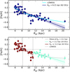 |
Fig. 1. Shape of radial [Fe/H] gradient. Upper panel: [Fe/H] vs RGC of our sample clusters. The blue line is a weighted linear regression model fit to the global trend and the shaded area shows the confidence interval. The cyan curve is the lowess fit. Bottom panel: [Fe/H] vs RGC with weighted linear regression model fits in two radial ranges, RGC ≤ 11.2 kpc (in brown) and RGC > 11.2 kpc (in turquoise). The shaded areas show the confidence intervals of the two fits and the dashed grey curves are the lowess models in the two intervals. The vertical grey line indicates the slope change point calculated by the elbow method. The dashed vertical and horizontal lines mark the location and abundance of the Sun. |
with a Pearson correlation coefficient (PCC) of −0.85. In the bottom panel of Fig. 1 we consider a two-slope fit, separating the inner and the outer regions. To choose the radius that separates the two regions, we applied the ELBOW method2 to find the critical point where the slope changes from high to low. Using the KNEEDLE algorithm (Satopaa et al. 2011), we found that the cutoff point is at RGC ∼ 11.2 kpc. The two-slope fitting provides a better representation of the behaviour of the outer clusters; however, because they are dominated by the inner clusters, the PCCs of the one-slope fit and of the inner part of the two-slope fit are very close, as shown below. Considering the two radial regions, RGC ≤ 11.2 kpc and RGC > 11.2 kpc, we obtain a steeper inner gradient
![Mathematical equation: $$ \begin{aligned} \mathrm{[Fe/H]} = -0.081(\pm 0.008)\times R_{\rm GC}+0.692(\pm 0.068) \end{aligned} $$](/articles/aa/full_html/2023/01/aa44957-22/aa44957-22-eq2.gif) (2)
(2)
with PCC = −0.86, and a much flatter outer plateau
![Mathematical equation: $$ \begin{aligned} \mathrm{[Fe/H]} = -0.044(\pm 0.014)\times R_{\rm GC}+0.376(\pm 0.178) \end{aligned} $$](/articles/aa/full_html/2023/01/aa44957-22/aa44957-22-eq3.gif) (3)
(3)
with a correlation coefficient PCC = −0.61. Our results are also reported in Table 1 to compare them with literature results. Our global slope is in good agreement with other works covering large radial regions, such as Netopil et al. (2022) and Spina et al. (2022). Our slope for the inner gradient, −0.081 dex kpc−1, is in agreement, within the uncertainties, with the gradients mapping the inner regions (Carrera et al. 2019; Spina et al. 2021; Myers et al. 2022; Donor et al. 2020; Zhang et al. 2021a).
3.2. Shape of average radial gradients per nucleosynthesis channel
Here and in the next sections we follow a purely observational approach to describe the elemental abundance and abundance ratio gradients. In comparing the gradients of the various elements, we expect different behaviour because they are sensitive to the timescales of the element production and to the variation in star formation histories and efficiencies along the disc extent, in particular the inside-out formation of the disc. Chemical evolution models can predict these variations accurately by taking into account, in a quantitative way, different channels of nucleosynthesis. An example is shown in Fig. 10 of Minchev et al. (2014), where the combination of the inside-out formation of the disc and the different timescales of the production of iron and of the α elements produces the growth in [α/Fe] in the outer parts of the disc. We plan a detailed comparison of the data presented in this paper with the predictions of a chemical evolution model (Molero et al. in prep.).
In Fig. 2 we present the radial distribution per group of elements. In each panel we computed the average abundance of the elements belonging to different groups, characterised by similar nucleosynthesis origins. This is clearly a rough approximation because even elements with similar origins (e.g. O and Mg) show differences (see discussion in McWilliam et al. 2008; Van der Swaelmen et al. 2023), but this approach can give us an idea of the average behaviour of each element class. In the figure we show the gradients of both [El/H] and [El/Fe]. In the first group, the α elements, we average the abundances of O, Mg, Ca, Si, and Ti. In this group we include Ti, not properly an α elements, but obtained from 48Cr, its radioactive α-element progenitor (see e.g. Clayton 2003). We exclude Na and Al, odd-Z elements synthesised in massive stars like the α elements, whose abundances might be altered by stellar evolution (Smiljanic et al. 2016). The overall α gradient is only slightly flatter than the [Fe/H] gradient, and, in the [α/Fe] versus RGC diagram, it shows a slight tendency to rise in the outer Galaxy, combined with a slight descent and high scatter in the inner disc. In the second group, the iron-peak elements, we considered Sc, V, Cr, Mn, Co, Ni, and Zn. For these elements we expect a behaviour similar to that of iron, and indeed the gradient [iron-peak/Fe] is quite flat reflecting the common production sites of Fe and these elements (cf. Myers et al. 2022). The apparent increase is due only to the outermost cluster. In the third group we combined the five s-process elements available in the final data release, namely Y, Zr, Ba, Ce, and La. Their cumulative gradient is slightly flatter than the [Fe/H] gradient. The strong metallicity dependence of the yields of the s-process elements comes into play, depressing the production with respect to iron in the inner Galaxy and increasing it in the outer Galaxy. Finally, in the fourth group we included the four r-process dominated elements (Eu, Nd, Mo, Pr), which are expected to be produced, in different percentages, by magnetically driven core collapse SNe or by compact binary mergers, such as neutron star-neutron star, neutron star-black hole, and black hole-black hole mergers (see Matteucci 2014), or by a combination of the two (see e.g. Simonetti et al. 2019; Molero et al. 2021; Van der Swaelmen et al. 2023). In both cases, the timescales of their production are short, as is shown by their flat [r/H] gradient and by the increasing trend of [r/Fe] versus RGC.
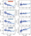 |
Fig. 2. Radial elemental gradients and average abundances for elements belonging to five nucleosynthesis channels as a function of RGC. The blue lines are the linear regression model fits, and the translucent bands around the regression lines are the confidence intervals for the regression estimate. The cyan curves are the lowess models. |
3.3. Shape of individual element gradients
In Figs. 3 and 4 we show the radial [El/H] and [El/Fe] gradients of all the individual elements grouped by their main nucleosynthesis channels. In Tables A.8 and A.9 we provide the coefficients of the weighted linear fits and the PCCs of the radial abundance ([El/H]) and abundance ratio ([El/Fe]) gradients for the whole radial range, and in the two radial regions (RGC ≤ 11.2 kpc and RGC > 11.2 kpc). Generally, the PCC is much larger for the steeper inner gradients and tends to be smaller for the flatter outer gradients.
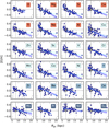 |
Fig. 3. Radial elemental gradients [El/H] as a function of RGC. The blue lines are linear regression model fits, the translucent bands around the regression lines describe a 95% bootstrap confidence interval, and the cyan curves are the lowess models. Each panel is colour-coded according to the nucleosynthesis channel (red: α and odd-Z elements; light cyan: iron-peak elements; cyan: s-process elements; dark cyan: r-process elements). |
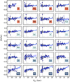 |
Fig. 4. Radial abundance ratio gradients [El/Fe] as a function of RGC. Symbols and colours are as in Fig. 3. |
α and odd-Z elements. In Fig. 3 and Table A.8, among the gradients of the first group (O, Mg, Ca, Si, Ti, Na, and Al) the gradient of [O/H] (RGC ≤ 11.2 kpc) is the flatter one. In that radial region, the slope of the [O/H] gradient is also flatter than that of Mg, the only other element in our sample expected to be produced by massive stars alone. As discussed in McWilliam et al. (2008), although the two elements are both produced by massive stars, they have different nucleosynthesis mechanisms with different impacts from stellar winds in their production. Oxygen is produced mostly during hydrostatic burning and expelled through stellar winds. Hence, its yield is expected to have a stronger dependence on the metallicity than the yields of the other α elements (e.g. Mg), which are synthesised mostly in the explosive phases. These differences are indeed confirmed by their gradients. In addition, for the other elements (e.g. Si, Ca, and Ti) there is a non-negligible fraction of their production in SN Ia (see e.g. Kobayashi et al. 2020). The last two elements of the group, Na and Al, are produced by massive stars, as are O and Mg (Kobayashi et al. 2020), but they also have a non-negligible contribution from low- and intermediate-mass stars, and, as discussed above, they might be affected by stellar evolution effects. In Fig. 4 we show the behaviour of the radial abundance gradients in the [El/Fe] versus RGC planes. Among the α elements, [O/Fe] shows the greatest growth towards the outer regions of the Galaxy, as expected by the inside-out formation of the Galactic disc. The other α elements and the two odd-Z elements have rather flat [El/Fe] gradients, since they have a non-negligible production in SN Ia, and thus similar timescales to iron.
Iron-peak elements. The group of iron-peak elements (Sc, V, Cr, Mn, Co, Ni, Zn) has a quite homogeneous behaviour in the [El/H]–RGC plane. The slopes of their gradients are very similar, around −0.08 dex kpc−1 for RGC ≤ 11.2 kpc and −0.025 dex kpc−1 for RGC > 11.2 kpc (see Table A.8). In the [El/Fe]–RGC plane, they are almost flat (see slopes in Table A.9 and Fig. 4). The abundances of Cu I are the most problematic values, as shown by the higher scatter of the results.
s-process elements. The s-process elements (Y, Zr, Ba, Ce, and La) have the most complex behaviour. In the [El/H]–RGC plane there is a non-negligible scatter in their gradients, as traced with clusters of all ages. Their overall gradients have typical slopes around −0.04 dex kpc−1, close to those of the α element gradients. In the [El/Fe]–RGC plane there is slight increase in the positive slope in the inner regions (RGC ≤ 11.2 kpc), and an almost flat trend for RGC > 11.2 kpc, with a decreasing trend for Zr and Ba.
r-process elements. The r-process elements (Eu, Nd, Mo, Pr) have mild overall gradients in the [El/H]–RGC plane, with typical slopes of ∼ − 0.02 dex kpc−1. In the [El/Fe]–RGC plane they have typical slopes of ∼+0.03 dex kpc−1, indicating for these elements shorter production timescales than those of iron. They are mainly produced by magnetically driven core collapse SNe or by compact binary mergers (Matteucci 2014), both on shorter timescales with respect to SN Ia.
4. Time evolution of radial abundance and abundance ratio gradients
Several stellar populations have been used to study the time evolution of the gradient: planetary nebulae (PNe), separated into age classes or combined with abundances of H II regions (e.g. Maciel et al. 2003, 2005; Stanghellini & Haywood 2010, 2018; Magrini et al. 2016); stars of different ages, in particular those with accurate age determination from asteroseismic observations (e.g. Anders et al. 2017). However, compared to other tracers, OCs have the advantage of being a homogeneous population whose ages and distances can be accurately determined, thereby resulting in an excellent tool to follow the time evolution of the abundance gradients.
Open clusters have been widely used to trace the changes in time of the Galactic metallicity and of its radial distribution (see e.g. Janes 1979; Twarog et al. 1997; Carraro et al. 1998; Friel et al. 2002; Chen et al. 2003; Magrini et al. 2009; Yong et al. 2012; Frinchaboy et al. 2013; Cunha et al. 2016; Spina et al. 2017, 2021; Donor et al. 2020; Zhong et al. 2020; Zhang et al. 2021a; Netopil et al. 2022; Myers et al. 2022). However, a common agreement on the time evolution of the gradient has not been reached to date, either because the cluster samples used in the past were small or because inhomogeneous data were often combined. The use of homogeneous data from large spectroscopic surveys proved to be fundamental (Spina et al. 2022; Myers et al. 2022). In Table 2 we show some recent literature results for the time evolution of the slope of the radial [Fe/H] gradient from open clusters. On average, the gradient shows a limited time evolution, with a slightly flatter gradient for the younger populations. The differences in the results presented in Table 2 are mainly due to the differences in the sampled radial regions and the considered age intervals, and when the younger clusters are included in the samples (see also Table 1).
Literature [Fe/H] gradients of open cluster samples divided in age bins.
Here we have the opportunity to revisit this issue with one of the largest samples of open clusters whose high-resolution spectra were homogeneously analysed.
4.1. Time evolution of [Fe/H] gradient
In Fig. 5, we present the radial [Fe/H] gradient of our open cluster sample, divided into three age bins. The age bins were chosen so as to have a similar number of clusters in each one. In Fig. 1 the dispersion observed in the overall [Fe/H] gradient, in particular in the inner part of the Galaxy, is mostly due to the mixing of clusters of different ages. For instance, between RGC 6.5–7.5 kpc the overall [Fe/H], including clusters of all ages, has a typical dispersion σ = 0.13 dex. The dispersion in metallicity of clusters belonging to each of the three age bins, at a given RGC, is smaller than the dispersion of the total sample (see Fig. 5). From Fig. 5 we see a remarkable evolution of the gradient with respect to what is suggested on the basis of simple chemical evolution arguments (i.e. the oldest populations should be less enriched than the youngest ones). In the radial range from RGC ∼ 6 to about 10 kpc the figure is evidence of a weird evolution of the gradient, where the youngest clusters more metal poor than the oldest ones. In addition, the gradient is flatter for the youngest clusters, while for RGC > 10 kpc the trend is reversed, and the younger clusters have similar [Fe/H] values to the older clusters. Similar conclusions were found in previous works based on open clusters (Carraro et al. 1998; Chen et al. 2003; Friel et al. 2002; Magrini et al. 2009; Spina et al. 2016; Randich et al. 2022, but see Netopil et al. 2022 for a contrasting result).
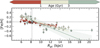 |
Fig. 5. Time evolution of radial [Fe/H] gradient. The circles are colour-coded by cluster ages. The three solid lines are the weighted linear regressions and the dashed curves are lowess models for the three age bins: age < 1 Gyr (red), 1 Gyr ≤ age < 3 Gyr (beige), and age ≥ 3 Gyr (green). |
The GaiaDR3 data also showed a similar behaviour. Recio-Blanco et al. (2023) presented two samples, the former composed of young field stars and the latter of stars in young open clusters. In both samples, they found a flattening of the gradient at recent epochs (a slope of −0.036 ± 0.002 dex kpc−1) in the sample of young and massive stars, to be compared with a slope of −0.055 ± 0.007 dex kpc−1 in the entire sample, in excellent agreement with our results (see Table 2 for more details about the gradient derived only with open clusters). Therefore, Recio-Blanco et al. (2023) concluded, from Gaia data alone, that both open clusters and field stars show a flattening of their radial [Fe/H] gradient in the more recent epochs of Milky Way evolution. On the other hand, the works of Spina et al. (2021), Netopil et al. (2022) and Myers et al. (2022) do not indicate large variations in the gradient slope with time (see Table 2), although the youngest clusters have lower [Fe/H] than the oldest ones. We discuss some hypotheses on the origin of the evolution of the gradient in Sect. 5.
4.2. Time evolution of average radial gradients per nucleosynthesis channel
In Fig. 6 we plot the radial abundance and abundance ratio gradients of the averaged elements in the four considered classes divided in the same age bins as Fig. 5. As above, Na, Al, and Cu are excluded from the average values. The [α/H] gradient has an evolution with time similar to the [Fe/H] gradient, but it is less pronounced: the oldest clusters are only slightly more enriched than the youngest ones. In addition, in the [α/Fe] versus RGC plot we find an important difference. For the older clusters (age > 1 Gyr), there is a slight decrease in the inner disc and a growth in the outer disc, as attested by the inside-out formation of the Galaxy and the different timescales of the formation of the α elements and Fe; instead, for the youngest clusters [α/Fe] is flat. For the iron-peak elements, we have, as for iron, a greater enrichment of [El/H] in the older clusters, while the youngest clusters have a flat gradient and are less enriched. Due to the common formation sites, the [El/Fe] gradients are almost flat at all ages. The situation of the s-process elements is more complex also with regard to their time evolution. The average [s/Fe] gradient does not show a remarkable variation with age in the inner region, while in the outer regions the youngest clusters are more enriched in s-process elements. This is likely due to the different timescales of their production and to the strong metallicity dependence of their yields (Casali et al. 2020b; Magrini et al. 2021b; Vescovi 2021; Viscasillas Vázquez et al. 2022). In the [s/Fe] plane the separation between the three age bins is clearer and is driven by the differences in [Fe/H] of the clusters. Finally, the r-process elements show a behaviour similar to that of the α elements, as expected due to their production on short timescales (see e.g. Matteucci 2014). On the [r/Fe] versus RGC plane the separation between the three age bins is likely driven by [Fe/H], as it is for the s-process elements.
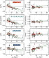 |
Fig. 6. Radial elemental gradients showing average abundances for elements belonging to four nucleosynthesis channels as a function of RGC. The lines are the linear regression model fit in every age bin, and the translucent bands around the regression lines show the confidence interval for the regression estimate. The dashed curves are the lowess models. The symbols and curves are colour-coded by cluster age as in Fig. 5. |
In summary, the average abundance and abundance ratio gradients of the four classes of elements considered have distinct time evolution. While for the iron-peak elements we recognise the same behaviour as [Fe/H], α elements and r-process elements have a limited time evolution of their [El/H] gradients, and their slopes remain almost constant with time. The behaviour of the s-process elements is the most complex, and their average gradient might hide this complexity. We describe the gradients element by element in Sect. 4.3.
4.3. Time evolution of individual element gradients
In Figs. 7 and 8 we present the abundance and abundance ratio gradients of all our sample elements, with open clusters divided into three age bins (0.1 Gyr < age < 1 Gyr, 1 Gyr ≤ age ≤ 3 Gyr, and age > 3 Gyr); in Fig. 9 we show the coefficients (slope-m1, y-intercept, and PCC) of the linear weighed fits (single slope) in the three age bins for the [El/H] gradients.
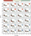 |
Fig. 7. [El/H] as a function of RGC. The clusters are divided into three age bins. The symbols and colours are as as in Fig. 5. |
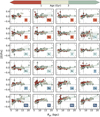 |
Fig. 8. [El/Fe] as a function of RGC. The clusters are divided into three age bins. The symbols and colours are as as in Fig. 5. |
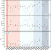 |
Fig. 9. Coefficients of the weighted linear fits of the abundance gradients: slope (top panel), intercepts (central panel), PCC (bottom panel). |
α elements. For the α and odd-Z elements our data show a limited time evolution of the slopes and intercepts of their gradients (see Fig. 9). In almost all cases, from O to Al, the shape of the gradient is basically unvaried with time in age range spanned by the youngest bin and the intermediate-age bin. The α elements do not appear to be significantly more abundant in either the youngest or the oldest population. In the two youngest age bins, the values of the intercepts of the gradients are in agreement within the uncertainties. In Fig. 8 the inner disc clusters at young ages show a flatter trend for their [α/Fe] with respect to the older clusters. The differences are mostly driven by variations in the denominator, Fe.
Iron-peak elements. In the group of the iron-peak elements, the time evolution is more marked. For Zn, Sc, V, Cr, Mn, Co, and Ni, the youngest clusters appear to be less enriched and they show a flatter gradient (see top and central panels of Fig. 9). The situation for Cu is less clear due to the high uncertainties on its abundance measurements and different nucleosynthetic origin. The [iron-peak/Fe] abundance ratios show almost flat gradients in the light of the common nucleosynthesis of iron and iron-peak elements.
s-process elements. The s-process elements are characterised by an inverse trend with respect to the α and iron-peak elements: the youngest clusters tend to have [El/H] abundances that are slightly higher than or equal to the older clusters. The s-process elements are mainly produced during He-shell burning in low-mass stars (1–3 M⊙; see e.g. Busso et al. 2001; Cristallo et al. 2011; Karakas & Lugaro 2016), which enrich the ISM at later times. Thus, the younger stellar populations formed from the ISM enriched by the products of low-mass stars will also be more abundant in s-process elements (see the values of the intercepts in the central panel of Fig. 9). In the gradients of [s/Fe] we recognise the strong age-dependence of those ratios (see e.g. D’Orazi et al. 2009; Maiorca et al. 2011, 2012). Unlike all the other gradients, for these abundance ratios we see a clear layering: the younger clusters have higher [s/Fe] and the older clusters are less enriched. This is particularly evident for [Y/Fe], [Ba/Fe], [La/Fe], and [Ce/Fe]; instead, [Zr/Fe] has a non-negligible r-process production and shows little time evolution in its [Zr/Fe] gradient.
r-process elements. Finally, similarly to α elements, r-process elements also do not show large variations with age for their gradient slopes and intercepts. For the r-process elements, the patterns are similar to those of the α elements, and they are mainly driven by the variations in Fe.
5. Origin of the gradient time evolution
From a purely observational point of view, our data confirm an extremely interesting result that is not immediately apparent. Focusing on Fig. 5 for the [Fe/H] gradient and on Fig. 7 for the individual abundance gradients, we can see a clear time evolution: older clusters (age > 1 Gyr) have steeper gradients and reach higher abundances, while younger clusters (age < 1 Gyr) have a flatter gradient with abundances below or equal to those of the older clusters. This evolution is peculiar in the context of chemical evolution, where we expect the chemical content to grow with time (in the closed-box approximation and in general in large galaxies, as our Milky Way, where the outflow is not considered dominant), and whose timescales generally do not predict such large changes in just 1 Gyr, especially during the latest phases of Galactic chemical evolution. Only a considerable infall of gas with lower metallicity could be invoked to explain the observations from a chemical evolution point of view (see e.g. the three infall models described in Spitoni et al. 2023).
In this section we investigate three hypotheses to explain the time evolution of the abundance gradients, evaluating some of their aspects. First, we discuss the infall of low-metallicity gas that triggered the latest episode of star formation in the thin disc (Ruiz-Lara et al. 2020) from which the youngest clusters were formed (Spitoni et al. 2019, 2023). Second, we look at migration and selective disruption effects (as suggested by e.g. Anders et al. 2017 and Spina et al. 2021, and more recently by Myers et al. 2022) in which the oldest clusters are more affected by migration, and preferentially originate in the inner disc where the typical metallicity is higher (see also Tarricq et al. 2022, for a characterisation of the orbits of clusters as a function of their age). Third, we consider artefacts due to spectral analysis in low-gravity giant stars (see e.g. Casali et al. 2020a; Zhang et al. 2021b; Spina et al. 2022; Carrera et al. 2022).
5.1. Effect of a recent infall
The work of Shanahan et al. (2019) claimed the discovery of compressed diffuse warm ionised medium in the spiral arm, upstream of the major star formation regions. Soler et al. (2020) found that the majority of the filamentary gas structures are aligned with the Galactic plane, although there are some significant exceptions of H I filaments mostly perpendicular to the Galactic plane. Perpendicular filaments correspond to locations in the disc where there is a significant accumulation of H II regions and supernova remnants. There is observational evidence of the presence of gas infall in the Galactic disc. The gas from outside can sustain the star formation in the spiral arms, and may have some effect on metallicity, diluting by the same amount the abundances of all elements and resulting in young stars with lower abundances in all elements. The chemical characteristics of the youngest and innermost clusters in the sample show a composition in α elements and r-process elements very similar to that of the oldest clusters of the sample and a depletion in the abundances of the iron-peak elements. These features can be informative in understanding the nature of the gas from which these clusters might have been formed. The dilution of the interstellar medium (ISM) with pristine gas causes a depletion of the same amount in all elements, as shown, for instance, in Spitoni et al. (2023) with their three-infall model. In this model, the thick disc originates from a first infall episode and the youngest thick-disc stars reach solar metallicities. A second infall, then, dilutes the gas, leading to a decrease in [Fe/H] and [El/H], while the [El/Fe] ratios remain substantially unchanged until the star formation activity resumes and new generations of SN II start polluting the ISM. Finally, a third recent infall episode is required that explains the chemical properties of the youngest metal-poor massive stars observed by Gaia (Gaia Collaboration 2023), while also being consistent with the recent enhanced star formation activity spotted by Ruiz-Lara et al. (2020) via an analysis of Gaia colour-magnitude diagrams. From the composition of our young clusters it can be inferred that the gas that formed them should have low metallicity (i.e. [Fe/H] < 0) at the solar radius. Furthermore, from Fig. 7 it appears that there is a diversification in the evolution with time of the gradients of the various elements. This seems to indicate that, if a large amount of gas infall is requested, it should also have a highly peculiar chemical composition. Full hydrodynamical simulations are required to investigate this scenario on a quantitative basis, both to identify the source of the gas and to explain its peculiar composition.
5.2. Migration and selection effects
Whether or not clusters are affected by radial migration as stars is not completely settled. Open clusters are more massive than single stars, and thus the effect of the interactions with perturbing structures, such as the spiral arms and the bar, might be different and less pronounced than for single stars (cf. Zhang et al. 2021a). Chemical evolution models have clearly pointed out that stellar migration has a non-negligible effect on the evolution with time of the gradient (see e.g. Minchev et al. 2013, 2014). Anders et al. (2017) attempted to explain the phenomenon of the time evolution of the gradient traced by open clusters by attributing the anomaly to the metallicities of the oldest clusters; their high metallicity for the current location was explained on the basis of their inner birth radius and the preferential migration direction from the inner to the outer disc. As discussed in Anders et al. (2017), Spina et al. (2021), Myers et al. (2022) and Gaia Collaboration (2023), metal-rich old clusters formed in the inner disc can survive only if they migrate outwards where the Galactic potential is less destructive, while those migrating inwards are quickly disrupted. Selection effects and migration might indeed affect the older populations, including clusters with age ≥ 3 Gyr, increasing the scatter in the gradient outlined by them and favouring the survival of metal-rich clusters moving from inner to outer disc regions. However, while stellar migration might have played a role for the oldest clusters, the intermediate-age clusters show a well-defined gradient, with small scatter along the whole disc, suggesting a very low probability that they have all migrated from the inner disc (see Fig. 5). Hence, the migration of old clusters can explain the higher abundances and the steeper gradient of the older populations, but it could hardly explain the differences between the gradients of the clusters in the young and intermediate-age bins, which had less time to migrate (see Frankel et al. 2018, and references therein).
5.3. Artefacts of spectral analysis in giants with low surface gravity
The unexpected shape of the gradient in the inner disc outlined by the youngest clusters is driven mainly by the metallicity derived in clusters that host only or mainly giant stars with low log g. The giant phase for young massive stars is characterised by high luminosities and low log g. In these stars, particularly those with high metallicity, spectral analysis is often prone to strong systematic effects that lead to a greater underestimation of metallicity, the lower the gravity. Casali et al. (2020a) carefully evaluated a number of possibilities to explain the origin of this issue, for example testing the use of photometric parameters instead of spectroscopic ones, the impact of non-local thermodynamic equilibrium (NLTE), the choice of the line list, the use of different atmosphere models, and the definition of the pseudo-continuum. In Fig. 10 we show [Fe/H] as a function of log g in a sample of OCs in which we observed numerous giant stars in a wide range of log g. The general trend indicates a decrease in [Fe/H] for stars with lower gravities. A clear example is shown by member stars in the cluster Trumpler 20, where stars with log g > 2.5 have [Fe/H] around 0.15, while those with lower gravity have [Fe/H] between 0 and 0.1. Therefore, when the number of stars with log g > 2.5 dominates, we have smaller effects in determining the average cluster abundance. Instead, in the case of young clusters where only stars with low gravity are present (e.g. NGC 6067, NGC 6259, NGC 6705), their [Fe/H] is most likely underestimated by a factor that depends on the typical gravity of the observed stars. The separation shown in Fig. 10 at log g = 2.5 is quite arbitrary, and it likely varies with metallicity, and it is set just to guide the eye. In addition, the effect may act differently for specific elements, due to the different photospheric regions in which their spectral lines forms and their relation with gravity.
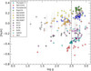 |
Fig. 10. [Fe/H] as a function of log g in giant star members of a sub-sample of OCs. The vertical line marks log g = 2.5. |
The trend of [Fe/H] versus log g is not specific to the analysis performed by Gaia-ESO but it is also found in the APOGEE and GALAH surveys, as shown in the Appendix (see Figs. A.1 and A.2), so it seems to be related to basic aspects, such as the treatment of opacity in model atmospheres or the use of semplified one-dimensional models. In Fig. A.3 we also show the comparison with the Gaia calibrated spectroscopic results, which are in excellent agreement with the Gaia-ESO data; however, as they are calibrated on open clusters, they display [Fe/H] values for young clusters similar to those of Gaia-ESO. In a forthcoming paper we will analyse the effects of the one-dimensional and three-dimensional approximations, and the possible impact of magnetic activity in young low-gravity giants by also studying its effects on various elements.
5.4. Giant stars in the youngest clusters
In the youngest clusters in our sample, we also observe a systematic increase in the measured microturbulent parameter (see Fig. 11). The origin of this phenomenon is still unknown; however, it closely resembles the effect that chromospheric activity has on the analysis of dwarf stars. Recent studies on solar twins have shown that strong absorption lines are intensified at high activity levels (Yana Galarza et al. 2019; Spina et al. 2020). This effect might be ascribed to the Zeeman broadening of absorption lines that form near the top of the stellar photosphere or even to the presence of cold stellar spots. However, other physical phenomena may be at work (Baratella et al. 2020, 2021). In any case, whatever the origin of this effect, the systemic rise in the microturbulent parameter for younger ages may cause biases in the abundance determinations for the youngest stars in our sample. Overestimating ξ implies underestimating both the effective temperature and the abundances of many elements, including Fe. To test this effect, we reanalysed the stars of the youngest cluster in our sample, NGC 6067. A recent work by Alonso-Santiago et al. (2017) gives for the giant stars in this cluster an average metallicity [Fe/H] = +0.19±0.05 consistent with the Galactic metallicity gradient. In their spectral analysis, the microturbulent parameter is set at the theoretical value of Adibekyan et al. (2012). We then re-analysed our sample of stars in NGC 6067, keeping ξ fixed at its theoretical value, and using the recommended parameters of Teff and log g from Gaia-ESO. In agreement with Alonso-Santiago et al. (2017), we obtain a super-solar metallicity, much higher than the recommended Gaia-ESO value, where ξ was derived from the spectral analysis and is higher than the theoretical value. Thus, the problem is most likely due to the determination of ξ, the physical origin of which might be linked to the magnetic activity of these stars.
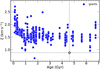 |
Fig. 11. Microturbulent parameter ξ as a function of the age of the cluster for individual giant cluster members. |
At present, however, there is scarce information about magnetic activity in giant stars that can lead us to firmly conclude that the effect is related to it. Recent results seem to support the possibility of a phase of enhanced activity for the most massive giant stars: following Schröder et al. (2018), we expect that chromospheric heating undergoes a remarkable reversal and revival as giant luminosity increases, and it becomes more important in young massive giants. In addition, these authors found the effect is enhanced in the most massive (and young) giant stars, which are generally more active. Similarly Konstantinova-Antova et al. (2014) found no evidence for magnetic giants below 1.7 M⊙, but they detect magnetic G and K giants with M > 1.7 M⊙ in the upper part of the RGB and in the AGB phase in more than 50% of their sample. In our sample, the youngest clusters with cool giants with log g < 2.5 have masses between 3.2 and 4.5 M⊙, thus all possibly hosting magnetic activity.
6. The true gradient
In this section our aim is to select stars for which the standard analysis, as performed by Gaia-ESO and other spectroscopic surveys, produces unbiased results. Moreover, we test the role of stellar dynamics, such as the Galactic warp and the cluster orbits.
6.1. Effect of biases introduced by spectral analysis
In Fig. 12 we show three versions of the gradient, limiting the samples to the inner radial region. In the top panel the gradient is drawn considering all clusters (equivalent to Fig. 5, but with symbols proportional to the number of members in each cluster and excluding clusters with fewer than three observed members). In the central panel we removed giant stars with log g < 2.5 in computing the cluster average metallicity. In the bottom panel of Fig. 12 we removed member giant stars with microturbulent velocity ξ > 1.8 km s−1. The results shown in the central and bottom panels are quite similar since the two removal conditions have similar effects, acting especially for clusters in which only low log g stars were observed (i.e. the youngest ones), which also have high ξ. The results of the linear fits are also shown in Table 3. The final effect is a gradient for the youngest populations which is very close to that of OCs with ages between 1 and 3 Gyr, pointing to a very limited evolution of the gradient in this amount of time. The intercept of the gradients of the young clusters rises in the two cases where stars have been removed for their log g or ξ with respect to the gradient computed with the full sample, thus solving the issue of the lack of enrichment of young populations. The limited evolution with time of the gradient might be a signature of the slow evolution and the lack of major interactions of the Milky Way with other galaxies in the latest few Gyr (see e.g. Sillero et al. 2017). The radial [Fe/H] gradient of their simulated galaxies, which are not experiencing strong disturbances, evolves smoothly without strong changes. The gradient of the oldest clusters (age > 3 Gyr) is almost unchanged by the removal of stars with low log g and high ξ. It remains steeper than that of the youngest populations, and with a positive offset towards higher metallicities, likely because of preferential cluster radial migration from metal-rich regions towards the Galaxy outskirts.
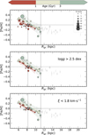 |
Fig. 12. Radial [Fe/H] gradient with all sample clusters divided into age bins (top panel), for members with log g > 2.5 (central panel), and for cluster members with ξ < 1.8 km s−1 (bottom panel). Open clusters are sized by the number of members and only clusters with three or more members are considered. The symbols and curves are colour-coded by cluster age as in Fig. 5. |
Radial gradients within 11.2 kpc with different restrictions (clusters with more than three members).
6.2. Effect of the warp
The outer part of the Galactic disc is not flat, but it is warping upwards in the north and downwards in the south. The warp of the Milky Way is not unique, but it is a typical characteristic of disc galaxies: about 50% of spiral galaxies have a warped disc (Reshetnikov & Combes 1998; Guijarro et al. 2010; Reshetnikov et al. 2016). Amôres et al. (2017) studied the time dependence of the structural parameters of the outer disc, including warp, flare, and disc truncation. They found evidence of time variation of the thin-disc scale length and of the shapes of the warp and flare (see also López-Corredoira et al. 2007). The reasons can be searched for in the misalignment between the disc and the dark halo surrounding the Galaxy or in the interaction with the Magellanic Clouds. As done in Spina et al. (2022), we corrected the RGC of our sample clusters considering the effect of the warp and its time dependence. The final effect is that older clusters suffer a larger radial correction than the younger ones because the disc of the Galaxy was shorter and more curved in the past. In Fig. 13 we show the radial [Fe/H] gradients in three age bins, with RGC corrected for the time-dependent shape of the warp. There is some reduction in the scatter in the region of the change in slope of the gradient, but still some old clusters have a remarkably low metallicity for their position at RGC∼10–12 kpc. Finally, the time-dependent correction for the Galactic warp has rather unrealistically moved the two outermost clusters of more than 20 kpc away from the Galactic centre. This is so because the correction for warp of older clusters is based on the model of the shape evolution of the Galaxy of Amôres et al. (2017), which has considerable uncertainties going back in time.
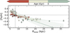 |
Fig. 13. Radial [Fe/H] gradients with all the sample clusters, colour-coded by the three age bins (one-slope linear weighted regressions, with the confidence levels indicated by the shaded areas). Their RGC are corrected for the time-dependent warp, as in Amôres et al. (2017). The dashed lines are the lowess fits. The symbols and curves are colour-coded by cluster age as in Fig. 5. |
6.3. Effect of radial migration (blurring)
We estimated the impact of radial migration, which, among its various effects, can also change the stellar or cluster orbits from circular to perturbed, with a relevant epicyclic component (blurring). Stars on perturbed orbits maintain their guiding radius and their angular momentum, but they can be found at different RGC along their orbits (Bird et al. 2012). Local encounters with molecular clouds (e.g. Spitzer & Schwarzschild 1953) or Lindblad resonance scattering between stars and spiral waves (e.g. Sellwood & Binney 2002) can also produce a change in the angular momentum and consequently in the stellar guiding radius. This effect is more difficult to evaluate, and probably affects to a lesser extent clusters that are more massive than individual stars (cf. Gustafsson et al. 2016).
We calculated the orbits of our cluster sample using the GALPY code, with the axisymmetric potential MWPOTENTIAL2014 (Bovy 2015). From the cluster orbits we computed their guiding radius, Rmean, defined as the average between the minimum and maximum radius (see e.g. Halle et al. 2015). We used Rmean to recompute the overall [Fe/H] gradients and their time evolution, considering the three age bins. The results are shown in Fig. 14. The high dispersion between 10 and 12 kpc is reduced using Rmean since some clusters located in that regions are likely coming from the outer regions.
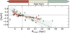 |
Fig. 14. Radial [Fe/H] gradients with all the sample clusters, colour-coded into three age bins, with Rmean obtained from orbit computation. The lines are the one-slope linear weighed regressions, with the confidence levels indicated by the shaded areas. The dashed lines are the lowess fits. The symbols and curves are colour-coded by cluster age as in Fig. 5. |
In Table 4 we report the three implementations of the [Fe/H] gradients: with the present-time RGC, with Rmean and with Rwarp. We provide both the overall gradient and the gradients in the three age bins. While the correction that takes into account the time-variable warp tends to flatten the gradients, especially for the sample of the oldest clusters, the gradients computed using Rmean are slightly steeper. It is likely that the model-dependent correction, which should reduce the effect of the warp, tends to overestimate the changes in the radius of the outer-disc old clusters, thus artificially flattening the slope. On the other hand, the gradients computed with RGC and Rmean are consistent within the errors, and also have similar PCCs (see Myers et al. 2022), indicating a secondary role of cluster migration in shaping the gradient. In the oldest bin, the effect of using Rmean improves the PCC of the fit, indicating, as expected, a more prominent role of migration for the oldest clusters.
Fitting coefficients of [Fe/H] = m1 ⋅ R + c for the total open cluster sample, and in the three investigated age bins, with RGC, Rwarp, and Rmean.
7. Summary and conclusions
In this paper we used the final data release of the Gaia-ESO survey to investigate the spatial distribution of the abundances and abundance ratios and their time evolution, as traced by open clusters (OCs). We can summarise our results in the following points:
-
Our sample of OCs traces a well-defined [Fe/H] gradient, which can be approximated with a single-slope fit [Fe/H] = −0.054(±0.004)×RGC + 0.474(±0.045), or with a two-slope fit, separating the inner region (RGC ≤ 11.2 kpc) and the outer one. Considering the two radial regions, we have an inner gradient, [Fe/H] = −0.081(±0.008)×RGC + 0.692(±0.068), and an outer plateau [Fe/H] = −0.044(±0.014)×RGC + 0.376(±0.178).
-
We derived radial abundance [El/H] and abundance ratio [El/Fe] gradients for additional 24 elements. We analysed both ratios in groups considering the average gradients of the α, iron-peak, s-process, and r-process elements, and for each individual element. All groups of elements and individual elements show negative [El/H] gradients. In the [El/Fe] versus RGC plane, α elements and r-process elements present slightly increasing trends, while iron-peak elements are almost flat. We find that s-process elements have a complex behaviour related to their nucleosynthesis.
-
We investigated the time evolution of the gradients, dividing the clusters into three age bins: age < 0.1 Gyr, 1 Gyr ≤ age ≤ 3 Gyr, and age > 3 Gyr. We found that the [Fe/H] of the youngest bin is characterised by a flatter slope, and for RGC ≤ 11.2 kpc by a lower metallicity. For the other elements, iron-peak elements have flatter gradients for the youngest clusters, while for α element and r-process elements the gradients are almost constant with age. The youngest clusters are more enhanced in s-process elements than the older ones, and have flatter gradients. We proposed some ideas to explain this evolution trend, for example chemical evolution and infall of metal-poor gas and stellar migration and selective disruptive events; finally, we considered the possible problem of the standard spectral analysis of low-gravity giant stars, as anticipated by Casali et al. (2020a) and Spina et al. (2022). We found that in the analysis of giants (log g < 2.5) we are likely to underestimate [Fe/H]. In addition, in the youngest giants at low log g, we might also overestimate the microturbulent velocity due to the possibly enhanced magnetic activity.
-
We evaluated the effect of the Galactic warp, considering also its shape in the past epochs, following Amôres et al. (2017). The gradients computed with distances deprojected in the warped disc tend to be flatter, especially for the older clusters. We also took into account stellar migration, computing the orbits of OCs. Using their Rmean instead of RGC, we computed the gradients. The scatter in the critical region around 10–12 kpc is reduced, but the overall shape of the gradient is almost unvaried within the errors.
We conclude that the radial [Fe/H] gradient as traced by OCs contains much important information on Galactic and stellar physics. Dividing clusters into age bins and carefully excluding young cool low-gravity giants allows us to trace the time-evolution of the radial metallicity gradient, which is very limited in time indicating a slow and stationary formation and evolution of the thin disc. The older clusters (age > 3 Gyr) still show a slightly steeper gradient, with an offset towards higher [Fe/H], likely related to preferential cluster migration from the inner to the outer disc. Upcoming instruments dedicated to spectroscopic surveys, such as WEAVE and 4MOST, will increase the number of clusters with a metallicity determination, but for the moment the Gaia-ESO data remains unbeaten in terms of spectral range and resolution, and consequently the number of measured chemical elements.
Acknowledgments
We would like to thank the referee for her/his careful reading and useful suggestions. Based on data products from observations made with ESO Telescopes at the La Silla Paranal Observatory under programmes 188.B-3002, 193.B-0936, and 197.B-1074. These data products have been processed by the Cambridge Astronomy Survey Unit (CASU) at the Institute of Astronomy, University of Cambridge, and by the FLAMES/UVES reduction team at INAF/Osservatorio Astrofisico di Arcetri. These data have been obtained from the Gaia-ESO Survey Data Archive, prepared and hosted by the Wide Field Astronomy Unit, Institute for Astronomy, University of Edinburgh, which is funded by the UK Science and Technology Facilities Council. This work was partly supported by the European Union FP7 programme through ERC grant number 320360 and by the Leverhulme Trust through grant RPG-2012-541.We acknowledge the support from INAF and Ministero dell’Istruzione, dell’Università e della Ricerca (MIUR) in the form of the grant “Premiale VLT 2012”. The results presented here benefit from discussions held during the Gaia-ESO workshops and conferences supported by the ESF (European Science Foundation) through the GREAT Research Network Programme. LM, SR, EF, GC, MVdS, GGS, AB acknowledges partial support from Premiale 2016 MITiC. MLLD and RS acknowledge support by the National Science Centre, Poland, project 2019/34/E/ST9/00133. MB is supported through the Lise Meitner grant from the Max Planck Society. We acknowledge support by the Collaborative Research centre SFB 881 (projects A5, A10), Heidelberg University, of the Deutsche Forschungsgemeinschaft (DFG, German Research Foundation). This project has received funding from the European Research Council (ERC) under the European Union’s Horizon 2020 research and innovation programme (Grant agreement No. 949173). TB was supported by grant No. 2018-04857 from the Swedish Research Council. UH acknowledges support from the Swedish National Space Agency (SNSA/Rymdstyrelsen). GC acknowledges support from the European Research Council Consolidator Grant funding scheme (project ASTEROCHRONOMETRY, G.A. n. 772293, http://www.asterochronometry.eu). CVV acknowledges support from “Direzione Generale per la diplomazia pubblica e culturale” of the “Ministero degli Affari Esteri e della Cooperazione Internazionale” and the “Istituto Italiano di Cultura in Vilnius”.
References
- Adibekyan, V. Z., Delgado Mena, E., Sousa, S. G., et al. 2012, A&A, 547, A36 [NASA ADS] [CrossRef] [EDP Sciences] [Google Scholar]
- Ahumada, A. V., Cignoni, M., Bragaglia, A., et al. 2013, MNRAS, 430, 221 [NASA ADS] [CrossRef] [Google Scholar]
- Alonso-Santiago, J., Negueruela, I., Marco, A., et al. 2017, MNRAS, 469, 1330 [NASA ADS] [CrossRef] [Google Scholar]
- Amôres, E. B., Robin, A. C., & Reylé, C. 2017, A&A, 602, A67 [NASA ADS] [CrossRef] [EDP Sciences] [Google Scholar]
- Anders, F., Chiappini, C., Minchev, I., et al. 2017, A&A, 600, A70 [NASA ADS] [CrossRef] [EDP Sciences] [Google Scholar]
- Arellano-Córdova, K. Z., Esteban, C., García-Rojas, J., & Méndez-Delgado, J. E. 2020, MNRAS, 496, 1051 [Google Scholar]
- Balser, D. S., Rood, R. T., Bania, T. M., & Anderson, L. D. 2011, ApJ, 738, 27 [NASA ADS] [CrossRef] [Google Scholar]
- Baratella, M., D’Orazi, V., Carraro, G., et al. 2020, A&A, 634, A34 [NASA ADS] [CrossRef] [EDP Sciences] [Google Scholar]
- Baratella, M., D’Orazi, V., Sheminova, V., et al. 2021, A&A, 653, A67 [NASA ADS] [CrossRef] [EDP Sciences] [Google Scholar]
- Bertelli Motta, C., Pasquali, A., Caffau, E., & Grebel, E. K. 2018, MNRAS, 480, 4314 [NASA ADS] [CrossRef] [Google Scholar]
- Biazzo, K., Randich, S., & Palla, F. 2011, A&A, 525, A35 [NASA ADS] [CrossRef] [EDP Sciences] [Google Scholar]
- Bird, J. C., Kazantzidis, S., & Weinberg, D. H. 2012, MNRAS, 420, 913 [NASA ADS] [CrossRef] [Google Scholar]
- Bovy, J. 2015, ApJS, 216, 29 [NASA ADS] [CrossRef] [Google Scholar]
- Bragaglia, A. 2008, Mem. Soc. Astron. It., 79, 365 [Google Scholar]
- Bragaglia, A., Sestito, P., Villanova, S., et al. 2008, A&A, 480, 79 [NASA ADS] [CrossRef] [EDP Sciences] [Google Scholar]
- Bragaglia, A., Alfaro, E. J., Flaccomio, E., et al. 2022, A&A, 659, A200 [NASA ADS] [CrossRef] [EDP Sciences] [Google Scholar]
- Bragança, G. A., Daflon, S., Lanz, T., et al. 2019, A&A, 625, A120 [NASA ADS] [CrossRef] [EDP Sciences] [Google Scholar]
- Busso, M., Gallino, R., Lambert, D. L., Travaglio, C., & Smith, V. V. 2001, ApJ, 557, 802 [CrossRef] [Google Scholar]
- Cantat-Gaudin, T., Anders, F., Castro-Ginard, A., et al. 2020, A&A, 640, A1 [NASA ADS] [CrossRef] [EDP Sciences] [Google Scholar]
- Carraro, G., & Chiosi, C. 1994, A&A, 287, 761 [NASA ADS] [Google Scholar]
- Carraro, G., Ng, Y. K., & Portinari, L. 1998, MNRAS, 296, 1045 [NASA ADS] [CrossRef] [Google Scholar]
- Carraro, G., Geisler, D., Villanova, S., Frinchaboy, P. M., & Majewski, S. R. 2007, A&A, 476, 217 [NASA ADS] [CrossRef] [EDP Sciences] [Google Scholar]
- Carrera, R., & Pancino, E. 2011, A&A, 535, A30 [NASA ADS] [CrossRef] [EDP Sciences] [Google Scholar]
- Carrera, R., Bragaglia, A., Cantat-Gaudin, T., et al. 2019, A&A, 623, A80 [NASA ADS] [CrossRef] [EDP Sciences] [Google Scholar]
- Carrera, R., Casamiquela, L., Bragaglia, A., et al. 2022, A&A, 663, A148 [NASA ADS] [CrossRef] [EDP Sciences] [Google Scholar]
- Casali, G., Magrini, L., Frasca, A., et al. 2020a, A&A, 643, A12 [NASA ADS] [CrossRef] [EDP Sciences] [Google Scholar]
- Casali, G., Spina, L., Magrini, L., et al. 2020b, A&A, 639, A127 [NASA ADS] [CrossRef] [EDP Sciences] [Google Scholar]
- Casamiquela, L., Carrera, R., Jordi, C., et al. 2016, MNRAS, 458, 3150 [NASA ADS] [CrossRef] [Google Scholar]
- Casamiquela, L., Carrera, R., Blanco-Cuaresma, S., et al. 2017, MNRAS, 470, 4363 [NASA ADS] [CrossRef] [Google Scholar]
- Casamiquela, L., Blanco-Cuaresma, S., Carrera, R., et al. 2019, MNRAS, 490, 1821 [NASA ADS] [CrossRef] [Google Scholar]
- Chen, L., & Hou, J. L. 2009, ASP Conf. Ser., 404, 343 [NASA ADS] [Google Scholar]
- Chen, L., Hou, J. L., & Wang, J. J. 2003, AJ, 125, 1397 [NASA ADS] [CrossRef] [Google Scholar]
- Clayton, D. 2003, Handbook of Isotopes in the Cosmos (Cambridge University Press) [Google Scholar]
- Cristallo, S., Piersanti, L., Straniero, O., et al. 2011, ApJS, 197, 17 [NASA ADS] [CrossRef] [Google Scholar]
- Cunha, K., Smith, V. V., & Lambert, D. L. 1998, ApJ, 493, 195 [NASA ADS] [CrossRef] [Google Scholar]
- Cunha, K., Frinchaboy, P. M., Souto, D., et al. 2016, Astron. Nachr., 337, 922 [NASA ADS] [CrossRef] [Google Scholar]
- da Silva, R., Crestani, J., Bono, G., et al. 2022, A&A, 661, A104 [NASA ADS] [CrossRef] [EDP Sciences] [Google Scholar]
- Daflon, S., & Cunha, K. 2004, ApJ, 617, 1115 [NASA ADS] [CrossRef] [Google Scholar]
- Dalton, G., Trager, S., Abrams, D. C., et al. 2018, SPIE, 10702, 388 [Google Scholar]
- de Jong, R. S., Agertz, O., Berbel, A. A., et al. 2019, The Messenger, 175, 3 [NASA ADS] [Google Scholar]
- De Silva, G. M., Freeman, K. C., Bland-Hawthorn, J., et al. 2015, MNRAS, 449, 2604 [NASA ADS] [CrossRef] [Google Scholar]
- Donati, P., Bragaglia, A., Cignoni, M., Cocozza, G., & Tosi, M. 2012, MNRAS, 424, 1132 [NASA ADS] [CrossRef] [Google Scholar]
- Donati, P., Beccari, G., Bragaglia, A., Cignoni, M., & Tosi, M. 2014, MNRAS, 437, 1241 [NASA ADS] [CrossRef] [Google Scholar]
- Donor, J., Frinchaboy, P. M., Cunha, K., et al. 2018, AJ, 156, 142 [NASA ADS] [CrossRef] [Google Scholar]
- Donor, J., Frinchaboy, P. M., Cunha, K., et al. 2020, AJ, 159, 199 [NASA ADS] [CrossRef] [Google Scholar]
- D’Orazi, V., Magrini, L., Randich, S., et al. 2009, ApJ, 693, L31 [Google Scholar]
- Esteban, C., Fang, X., García-Rojas, J., & Toribio San Cipriano, L. 2017, MNRAS, 471, 987 [NASA ADS] [CrossRef] [Google Scholar]
- Frankel, N., Rix, H.-W., Ting, Y.-S., Ness, M., & Hogg, D. W. 2018, ApJ, 865, 96 [NASA ADS] [CrossRef] [Google Scholar]
- Friel, E. D. 1995, ARA&A, 33, 381 [Google Scholar]
- Friel, E. D., & Janes, K. A. 1993, A&A, 267, 75 [NASA ADS] [Google Scholar]
- Friel, E. D., Janes, K. A., Tavarez, M., et al. 2002, AJ, 124, 2693 [NASA ADS] [CrossRef] [Google Scholar]
- Friel, E. D., Jacobson, H. R., & Pilachowski, C. A. 2010, AJ, 139, 1942 [NASA ADS] [CrossRef] [Google Scholar]
- Frinchaboy, P. M., Thompson, B., Jackson, K. M., et al. 2013, ApJ, 777, L1 [NASA ADS] [CrossRef] [Google Scholar]
- Fu, X., Bragaglia, A., Liu, C., et al. 2022, A&A, 668, A4 [NASA ADS] [CrossRef] [EDP Sciences] [Google Scholar]
- Gaia Collaboration (Brown, A. G. A., et al.) 2016a, A&A, 595, A2 [NASA ADS] [CrossRef] [EDP Sciences] [Google Scholar]
- Gaia Collaboration (Prusti, T., et al.) 2016b, A&A, 595, A1 [NASA ADS] [CrossRef] [EDP Sciences] [Google Scholar]
- Gaia Collaboration (Brown, A. G. A., et al.) 2018, A&A, 616, A1 [NASA ADS] [CrossRef] [EDP Sciences] [Google Scholar]
- Gaia Collaboration (Brown, A. G. A., et al.) 2021, A&A, 649, A1 [NASA ADS] [CrossRef] [EDP Sciences] [Google Scholar]
- Gaia Collaboration (Recio-Blanco, A., et al.) 2023, A&A, in press, https://doi.org/10.1051/0004-6361/202243511 [Google Scholar]
- Genovali, K., Lemasle, B., Bono, G., et al. 2014, A&A, 566, A37 [NASA ADS] [CrossRef] [EDP Sciences] [Google Scholar]
- Genovali, K., Lemasle, B., da Silva, R., et al. 2015, A&A, 580, A17 [NASA ADS] [CrossRef] [EDP Sciences] [Google Scholar]
- Gilmore, G., Randich, S., Asplund, M., et al. 2012, The Messenger, 147, 25 [NASA ADS] [Google Scholar]
- Gilmore, G., Randich, S., Worley, C. C., et al. 2022, A&A, 666, A120 [NASA ADS] [CrossRef] [EDP Sciences] [Google Scholar]
- Grevesse, N., Asplund, M., & Sauval, A. J. 2007, Space Sci. Rev., 130, 105 [Google Scholar]
- Guijarro, A., Peletier, R. F., Battaner, E., et al. 2010, A&A, 519, A53 [NASA ADS] [CrossRef] [EDP Sciences] [Google Scholar]
- Gustafsson, B., Church, R. P., Davies, M. B., & Rickman, H. 2016, A&A, 593, A85 [NASA ADS] [CrossRef] [EDP Sciences] [Google Scholar]
- Halle, A., Di Matteo, P., Haywood, M., & Combes, F. 2015, A&A, 578, A58 [NASA ADS] [CrossRef] [EDP Sciences] [Google Scholar]
- Henry, R. B. C., Kwitter, K. B., Jaskot, A. E., et al. 2010, ApJ, 724, 748 [NASA ADS] [CrossRef] [Google Scholar]
- Hourihane, A. P., Franis, P., Worley, C. C., Magrini, L., & Gaia-ESO Consortium 2022, A&A, in press [Google Scholar]
- Jackson, R. J., Jeffries, R. D., Wright, N. J., et al. 2022, MNRAS, 509, 1664 [Google Scholar]
- Jacobson, H. R., Friel, E. D., Jílková, L., et al. 2016, A&A, 591, A37 [NASA ADS] [CrossRef] [EDP Sciences] [Google Scholar]
- Janes, K. A. 1979, ApJS, 39, 135 [NASA ADS] [CrossRef] [Google Scholar]
- Janes, K. A., Tilley, C., & Lynga, G. 1988, AJ, 95, 771 [NASA ADS] [CrossRef] [Google Scholar]
- Karakas, A. I., & Lugaro, M. 2016, ApJ, 825, 26 [NASA ADS] [CrossRef] [Google Scholar]
- Kobayashi, C., Karakas, A. I., & Lugaro, M. 2020, ApJ, 900, 179 [Google Scholar]
- Konstantinova-Antova, R., Aurière, M., Charbonnel, C., et al. 2014, in Magnetic Fields throughout Stellar Evolution, eds. P. Petit, M. Jardine, & H. C. Spruit, 302, 373 [NASA ADS] [Google Scholar]
- Kovtyukh, V., Lemasle, B., Bono, G., et al. 2022, MNRAS, 510, 1894 [Google Scholar]
- Lemasle, B., François, P., Bono, G., et al. 2007, A&A, 467, 283 [NASA ADS] [CrossRef] [EDP Sciences] [Google Scholar]
- Lemasle, B., François, P., Piersimoni, A., et al. 2008, A&A, 490, 613 [NASA ADS] [CrossRef] [EDP Sciences] [Google Scholar]
- Lemasle, B., François, P., Genovali, K., et al. 2013, A&A, 558, A31 [NASA ADS] [CrossRef] [EDP Sciences] [Google Scholar]
- Liu, F., Asplund, M., Yong, D., et al. 2016, MNRAS, 463, 696 [NASA ADS] [CrossRef] [Google Scholar]
- López-Corredoira, M., Momany, Y., Zaggia, S., & Cabrera-Lavers, A. 2007, A&A, 472, L47 [NASA ADS] [CrossRef] [EDP Sciences] [Google Scholar]
- Luck, R. E. 2018, AJ, 156, 171 [Google Scholar]
- Maciel, W. J., Costa, R. D. D., & Uchida, M. M. M. 2003, A&A, 397, 667 [NASA ADS] [CrossRef] [EDP Sciences] [Google Scholar]
- Maciel, W. J., Lago, L. G., & Costa, R. D. D. 2005, A&A, 433, 127 [NASA ADS] [CrossRef] [EDP Sciences] [Google Scholar]
- Magrini, L., Sestito, P., Randich, S., & Galli, D. 2009, A&A, 494, 95 [NASA ADS] [CrossRef] [EDP Sciences] [Google Scholar]
- Magrini, L., Randich, S., Zoccali, M., et al. 2010, A&A, 523, A11 [NASA ADS] [CrossRef] [EDP Sciences] [Google Scholar]
- Magrini, L., Coccato, L., Stanghellini, L., Casasola, V., & Galli, D. 2016, A&A, 588, A91 [NASA ADS] [CrossRef] [EDP Sciences] [Google Scholar]
- Magrini, L., Randich, S., Kordopatis, G., et al. 2017, A&A, 603, A2 [NASA ADS] [CrossRef] [EDP Sciences] [Google Scholar]
- Magrini, L., Lagarde, N., Charbonnel, C., et al. 2021a, A&A, 651, A84 [NASA ADS] [CrossRef] [EDP Sciences] [Google Scholar]
- Magrini, L., Vescovi, D., Casali, G., et al. 2021b, A&A, 646, L2 [EDP Sciences] [Google Scholar]
- Maiorca, E., Randich, S., Busso, M., Magrini, L., & Palmerini, S. 2011, ApJ, 736, 120 [NASA ADS] [CrossRef] [Google Scholar]
- Maiorca, E., Magrini, L., Busso, M., et al. 2012, ApJ, 747, 53 [Google Scholar]
- Majewski, S. R., Schiavon, R. P., Frinchaboy, P. M., et al. 2017, AJ, 154, 94 [NASA ADS] [CrossRef] [Google Scholar]
- Matteucci, F. 2014, The Origin of the Galaxy and Local Group, Saas-Fee Advanced Course (Berlin, Heidelberg: Springer-Verlag), 37, 145 [NASA ADS] [CrossRef] [Google Scholar]
- Mayor, M. 1976, A&A, 48, 301 [NASA ADS] [Google Scholar]
- McWilliam, A., Matteucci, F., Ballero, S., et al. 2008, AJ, 136, 367 [NASA ADS] [CrossRef] [Google Scholar]
- Méndez-Delgado, J. E., Amayo, A., Arellano-Córdova, K. Z., et al. 2022, MNRAS, 510, 4436 [CrossRef] [Google Scholar]
- Minchev, I., Chiappini, C., & Martig, M. 2013, A&A, 558, A9 [CrossRef] [EDP Sciences] [Google Scholar]
- Minchev, I., Chiappini, C., & Martig, M. 2014, A&A, 572, A92 [CrossRef] [EDP Sciences] [Google Scholar]
- Molero, M., Simonetti, P., Matteucci, F., & della Valle, M. 2021, MNRAS, 500, 1071 [Google Scholar]
- Myers, N., Donor, J., Spoo, T., et al. 2022, AJ, 164, 85 [NASA ADS] [CrossRef] [Google Scholar]
- Netopil, M., Oralhan, İ. A., Çakmak, H., Michel, R., & Karataş, Y. 2022, MNRAS, 509, 421 [Google Scholar]
- Önehag, A., Korn, A., Gustafsson, B., Stempels, E., & Vandenberg, D. A. 2011, A&A, 528, A85 [NASA ADS] [CrossRef] [EDP Sciences] [Google Scholar]
- Önehag, A., Gustafsson, B., & Korn, A. 2014, A&A, 562, A102 [NASA ADS] [CrossRef] [EDP Sciences] [Google Scholar]
- Padgett, D. L. 1996, ApJ, 471, 847 [NASA ADS] [CrossRef] [Google Scholar]
- Pancino, E., Carrera, R., Rossetti, E., & Gallart, C. 2010, A&A, 511, A56 [NASA ADS] [CrossRef] [EDP Sciences] [Google Scholar]
- Pancino, E., Lardo, C., Altavilla, G., et al. 2017, A&A, 598, A5 [NASA ADS] [CrossRef] [EDP Sciences] [Google Scholar]
- Pasquini, L., Avila, G., Blecha, A., et al. 2002, The Messenger, 110, 1 [Google Scholar]
- Pedicelli, S., Bono, G., Lemasle, B., et al. 2009, A&A, 504, 81 [NASA ADS] [CrossRef] [EDP Sciences] [Google Scholar]
- Peimbert, M., Torres-Peimbert, S., & Rayo, J. F. 1978, ApJ, 220, 516 [NASA ADS] [CrossRef] [Google Scholar]
- Perinotto, M., & Morbidelli, L. 2006, MNRAS, 372, 45 [NASA ADS] [CrossRef] [Google Scholar]
- Randich, S., Sestito, P., & Pallavicini, R. 2003, A&A, 399, 133 [NASA ADS] [CrossRef] [EDP Sciences] [Google Scholar]
- Randich, S., Bragaglia, A., Pastori, L., et al. 2005, The Messenger, 121, 18 [NASA ADS] [Google Scholar]
- Randich, S., Sestito, P., Primas, F., Pallavicini, R., & Pasquini, L. 2006, A&A, 450, 557 [NASA ADS] [CrossRef] [EDP Sciences] [Google Scholar]
- Randich, S., Primas, F., Pasquini, L., Sestito, P., & Pallavicini, R. 2007, A&A, 469, 163 [NASA ADS] [CrossRef] [EDP Sciences] [Google Scholar]
- Randich, S., Gilmore, G., & Gaia-ESO, C. 2013, The Messenger, 154, 47 [NASA ADS] [Google Scholar]
- Randich, S., Gilmore, G., Magrini, L., et al. 2022, A&A, 666, A121 [NASA ADS] [CrossRef] [EDP Sciences] [Google Scholar]
- Recio-Blanco, A., de Laverny, P., Palicio, P. A., et al. 2023, A&A, in press https://doi.org/10.1051/0004-6361/202243750 [Google Scholar]
- Reddy, A. B. S., Lambert, D. L., & Giridhar, S. 2016, MNRAS, 463, 4366 [NASA ADS] [CrossRef] [Google Scholar]
- Reshetnikov, V., & Combes, F. 1998, A&A, 337, 9 [NASA ADS] [Google Scholar]
- Reshetnikov, V. P., Mosenkov, A. V., Moiseev, A. V., Kotov, S. S., & Savchenko, S. S. 2016, MNRAS, 461, 4233 [NASA ADS] [CrossRef] [Google Scholar]
- Rolleston, W. R. J., Smartt, S. J., Dufton, P. L., & Ryans, R. S. I. 2000, A&A, 363, 537 [NASA ADS] [Google Scholar]
- Romano, D., & Matteucci, F. 2007, MNRAS, 378, L59 [NASA ADS] [Google Scholar]
- Ruiz-Lara, T., Gallart, C., Bernard, E. J., & Cassisi, S. 2020, Nat. Astron., 4, 965 [NASA ADS] [CrossRef] [Google Scholar]
- Sacco, G. G., Morbidelli, L., Franciosini, E., et al. 2014, A&A, 565, A113 [NASA ADS] [CrossRef] [EDP Sciences] [Google Scholar]
- Satopaa, V., Albrecht, J., Irwin, D., & Raghavan, B. 2011, in 2011 31st International Conference on Distributed Computing Systems Workshops, 166 [CrossRef] [Google Scholar]
- Schröder, K. P., Schmitt, J. H. M. M., Mittag, M., Gómez Trejo, V., & Jack, D. 2018, MNRAS, 480, 2137 [CrossRef] [Google Scholar]
- Sellwood, J. A., & Binney, J. J. 2002, MNRAS, 336, 785 [Google Scholar]
- Sestito, P., Randich, S., Mermilliod, J. C., & Pallavicini, R. 2003, A&A, 407, 289 [NASA ADS] [CrossRef] [EDP Sciences] [Google Scholar]
- Sestito, P., Randich, S., & Pallavicini, R. 2004, A&A, 426, 809 [NASA ADS] [CrossRef] [EDP Sciences] [Google Scholar]
- Sestito, P., Randich, S., & Pallavicini, R. 2006, in Chemical Abundances and Mixing in Stars in the Milky Way and its Satellites, 179 [CrossRef] [Google Scholar]
- Sestito, P., Randich, S., & Bragaglia, A. 2007, A&A, 465, 185 [NASA ADS] [CrossRef] [EDP Sciences] [Google Scholar]
- Sestito, P., Palla, F., & Randich, S. 2008a, A&A, 487, 965 [NASA ADS] [CrossRef] [EDP Sciences] [Google Scholar]
- Sestito, P., Bragaglia, A., Randich, S., et al. 2008b, A&A, 488, 943 [NASA ADS] [CrossRef] [EDP Sciences] [Google Scholar]
- Shanahan, R., Lemmer, S. J., Stil, J. M., et al. 2019, ApJ, 887, L7 [NASA ADS] [CrossRef] [Google Scholar]
- Sillero, E., Tissera, P. B., Lambas, D. G., & Michel-Dansac, L. 2017, MNRAS, 472, 4404 [NASA ADS] [CrossRef] [Google Scholar]
- Simonetti, P., Matteucci, F., Greggio, L., & Cescutti, G. 2019, MNRAS, 486, 2896 [NASA ADS] [CrossRef] [Google Scholar]
- Smiljanic, R., Korn, A. J., Bergemann, M., et al. 2014, A&A, 570, A122 [NASA ADS] [CrossRef] [EDP Sciences] [Google Scholar]
- Smiljanic, R., Romano, D., Bragaglia, A., et al. 2016, A&A, 589, A115 [NASA ADS] [CrossRef] [EDP Sciences] [Google Scholar]
- Soler, J. D., Beuther, H., Syed, J., et al. 2020, A&A, 642, A163 [NASA ADS] [CrossRef] [EDP Sciences] [Google Scholar]
- Souto, D., Allende Prieto, C., Cunha, K., et al. 2019, ApJ, 874, 97 [NASA ADS] [CrossRef] [Google Scholar]
- Spina, L., Meléndez, J., Karakas, A. I., et al. 2016, A&A, 593, A125 [NASA ADS] [CrossRef] [EDP Sciences] [Google Scholar]
- Spina, L., Randich, S., Magrini, L., et al. 2017, A&A, 601, A70 [NASA ADS] [CrossRef] [EDP Sciences] [Google Scholar]
- Spina, L., Nordlander, T., Casey, A. R., et al. 2020, ApJ, 895, 52 [Google Scholar]
- Spina, L., Ting, Y. S., De Silva, G. M., et al. 2021, MNRAS, 503, 3279 [CrossRef] [Google Scholar]
- Spina, L., Magrini, L., & Cunha, K. 2022, Universe, 8, 87 [NASA ADS] [CrossRef] [Google Scholar]
- Spitoni, E., Silva Aguirre, V., Matteucci, F., Calura, F., & Grisoni, V. 2019, A&A, 623, A60 [NASA ADS] [CrossRef] [EDP Sciences] [Google Scholar]
- Spitoni, E., Recio-Blanco, A., de Laverny, P., et al. 2023, A&A, in press https://doi.org/10.1051/0004-6361/202244349 [Google Scholar]
- Spitzer, L. J., & Schwarzschild, M. 1953, ApJ, 118, 106 [NASA ADS] [CrossRef] [Google Scholar]
- Stanghellini, L., & Haywood, M. 2010, ApJ, 714, 1096 [NASA ADS] [CrossRef] [Google Scholar]
- Stanghellini, L., & Haywood, M. 2018, ApJ, 862, 45 [Google Scholar]
- Tarricq, Y., Soubiran, C., Casamiquela, L., et al. 2022, A&A, 659, A59 [NASA ADS] [CrossRef] [EDP Sciences] [Google Scholar]
- Twarog, B. A., Ashman, K. M., & Anthony-Twarog, B. J. 1997, AJ, 114, 2556 [NASA ADS] [CrossRef] [Google Scholar]
- Van der Swaelmen, M., Viscasillas Vázquez, C., Cescutti, G., et al. 2023, A&A, in press https://doi.org/10.1051/0004-6361/202243764 [NASA ADS] [CrossRef] [EDP Sciences] [Google Scholar]
- Vescovi, D. 2021, Universe, 8, 16 [NASA ADS] [CrossRef] [Google Scholar]
- Viscasillas Vázquez, C., Magrini, L., Casali, G., et al. 2022, A&A, 660, A135 [NASA ADS] [CrossRef] [EDP Sciences] [Google Scholar]
- von Hippel, T., & Sarajedini, A. 1998, AJ, 116, 1789 [NASA ADS] [CrossRef] [Google Scholar]
- Woosley, S. E., & Weaver, T. A. 1995, ApJS, 101, 181 [Google Scholar]
- Yana Galarza, J., Meléndez, J., Lorenzo-Oliveira, D., et al. 2019, MNRAS, 490, L86 [Google Scholar]
- Yong, D., Carney, B. W., & Teixera de Almeida, M. L. 2005, AJ, 130, 597 [Google Scholar]
- Yong, D., Carney, B. W., & Friel, E. D. 2012, AJ, 144, 95 [Google Scholar]
- Zhang, H., Chen, Y., & Zhao, G. 2021a, ApJ, 919, 52 [NASA ADS] [CrossRef] [Google Scholar]
- Zhang, R., Lucatello, S., Bragaglia, A., et al. 2021b, A&A, 654, A77 [NASA ADS] [CrossRef] [EDP Sciences] [Google Scholar]
- Zhao, G., Zhao, Y.-H., Chu, Y.-Q., Jing, Y.-P., & Deng, L.-C. 2012, Res. Astron. Astrophys., 12, 723 [NASA ADS] [CrossRef] [Google Scholar]
- Zhong, J., Chen, L., Wu, D., et al. 2020, A&A, 640, A127 [NASA ADS] [CrossRef] [EDP Sciences] [Google Scholar]
Appendix A: Additional material
A.1. Effect of analysis of low-gravity giants in other spectroscopic surveys
In this section, we show the metallicity as a function of log g for a sample of members of open clusters in common between Gaia-ESO and GALAH DR3 and between Gaia-ESO and APOGEE DR17. In Fig. A.1 we present the results of GALAH and in Fig. A.2 the results of APOGEE DR17. In both figures a trend of decreasing metallicity as gravity declines can be seen. In Fig. A.3 we plot the results of Gaia RVS (Recio-Blanco et al. 2023) for stars in common with Gaia-ESO.
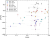 |
Fig. A.1. Metallicity vs gravity of a sample of stars in clusters in common between Gaia-ESO and GALAH DR3. The [Fe/H] and log g vlaues from GALAH DR3 and from Gaia-ESO are shown with different symbols, as indicated in the legend. |
A.2. Individual element gradients: Abundances and parameters of linear weighed regressions fits
In this section we provide tables with the solar and M67 abundances (Table A.1), with coefficients of the linear weighed regressions fitting for the two radial regions (Tables A.8 and A.9) and for the three age bins (Tables A.10 and A.11).
The average [El/H] and [El/Fe] of our cluster sample for the α elements are listed in Table A.2, for the odd elements in Table A.3, for the iron-peak elements in Table A.4, for the s-process elements in Table A.5, and for the r-process elements in Table A.6. In Table A.7 we show the number of member stars whose abundances have been used in each cluster per element.
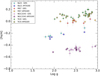 |
Fig. A.2. Metallicity vs gravity of a sample of stars in clusters in common between Gaia-ESO and APOGEE DR17. The [Fe/H] and log g values from APOGEE DR17 and from Gaia-ESO are shown with different symbols, as indicated in the legend. |
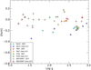 |
Fig. A.3. Metallicity vs gravity of a sample of stars in clusters in common between Gaia-ESO and Gaia RVS (Recio-Blanco et al. 2023). The [Fe/H] and log g values from Gaia and from Gaia-ESO are shown with different symbols, as indicated in the legend. |
IDR6 solar and M67 abundances.
Average [α/H] and [α/Fe] for our sample of open clusters. The age (Gyr) and RGC (kpc) are from Cantat-Gaudin et al. (2020) and [Fe/H] is from Randich et al. (2022).
Average [odd/H] and [odd/Fe] for our sample of open clusters. The age (Gyr) and RGC (kpc) are from Cantat-Gaudin et al. (2020) and [Fe/H] is from Randich et al. (2022).
Average [iron peak/H] and [iron peak/Fe] for our sample of open clusters. The age (Gyr) and RGC (kpc) are from Cantat-Gaudin et al. (2020) and [Fe/H] is from Randich et al. (2022).
Average [s/H] and [s/Fe] for our sample of open clusters. The age (Gyr) and RGC (kpc) are from Cantat-Gaudin et al. (2020) and [Fe/H] is from Randich et al. (2022).
Average [r/H] and [r/Fe] for our sample of open clusters. The age (Gyr) and RGC (kpc) are from Cantat-Gaudin et al. (2020) and [Fe/H] is from Randich et al. (2022).
Number of member stars in each cluster and for each element used in this work.
Linear weighed regression fitting coefficients of [El/H] = m1 ⋅ RGC + c for the open clusters in the two investigated galactocentric regions and in the whole distance range.
Linear weighed regression fitting coefficients of [El/Fe] = m1 ⋅ RGC + c for the open clusters in the two investigated galactocentric regions and in the whole distance range.
Linear weighed regression fitting coefficients of [El/H] = m1 ⋅ RGC + c for the open clusters in the three investigated age bins.
Linear weighed regression fitting coefficients of [El/Fe] = m1 ⋅ RGC + c for the open clusters in the three investigated age bins.
All Tables
Slopes of the [Fe/H] gradient from open cluster samples, from the recent literature.
Radial gradients within 11.2 kpc with different restrictions (clusters with more than three members).
Fitting coefficients of [Fe/H] = m1 ⋅ R + c for the total open cluster sample, and in the three investigated age bins, with RGC, Rwarp, and Rmean.
Average [α/H] and [α/Fe] for our sample of open clusters. The age (Gyr) and RGC (kpc) are from Cantat-Gaudin et al. (2020) and [Fe/H] is from Randich et al. (2022).
Average [odd/H] and [odd/Fe] for our sample of open clusters. The age (Gyr) and RGC (kpc) are from Cantat-Gaudin et al. (2020) and [Fe/H] is from Randich et al. (2022).
Average [iron peak/H] and [iron peak/Fe] for our sample of open clusters. The age (Gyr) and RGC (kpc) are from Cantat-Gaudin et al. (2020) and [Fe/H] is from Randich et al. (2022).
Average [s/H] and [s/Fe] for our sample of open clusters. The age (Gyr) and RGC (kpc) are from Cantat-Gaudin et al. (2020) and [Fe/H] is from Randich et al. (2022).
Average [r/H] and [r/Fe] for our sample of open clusters. The age (Gyr) and RGC (kpc) are from Cantat-Gaudin et al. (2020) and [Fe/H] is from Randich et al. (2022).
Number of member stars in each cluster and for each element used in this work.
Linear weighed regression fitting coefficients of [El/H] = m1 ⋅ RGC + c for the open clusters in the two investigated galactocentric regions and in the whole distance range.
Linear weighed regression fitting coefficients of [El/Fe] = m1 ⋅ RGC + c for the open clusters in the two investigated galactocentric regions and in the whole distance range.
Linear weighed regression fitting coefficients of [El/H] = m1 ⋅ RGC + c for the open clusters in the three investigated age bins.
Linear weighed regression fitting coefficients of [El/Fe] = m1 ⋅ RGC + c for the open clusters in the three investigated age bins.
All Figures
|
Fig. 1. Shape of radial [Fe/H] gradient. Upper panel: [Fe/H] vs RGC of our sample clusters. The blue line is a weighted linear regression model fit to the global trend and the shaded area shows the confidence interval. The cyan curve is the lowess fit. Bottom panel: [Fe/H] vs RGC with weighted linear regression model fits in two radial ranges, RGC ≤ 11.2 kpc (in brown) and RGC > 11.2 kpc (in turquoise). The shaded areas show the confidence intervals of the two fits and the dashed grey curves are the lowess models in the two intervals. The vertical grey line indicates the slope change point calculated by the elbow method. The dashed vertical and horizontal lines mark the location and abundance of the Sun. |
| In the text | |
|
Fig. 2. Radial elemental gradients and average abundances for elements belonging to five nucleosynthesis channels as a function of RGC. The blue lines are the linear regression model fits, and the translucent bands around the regression lines are the confidence intervals for the regression estimate. The cyan curves are the lowess models. |
| In the text | |
|
Fig. 3. Radial elemental gradients [El/H] as a function of RGC. The blue lines are linear regression model fits, the translucent bands around the regression lines describe a 95% bootstrap confidence interval, and the cyan curves are the lowess models. Each panel is colour-coded according to the nucleosynthesis channel (red: α and odd-Z elements; light cyan: iron-peak elements; cyan: s-process elements; dark cyan: r-process elements). |
| In the text | |
|
Fig. 4. Radial abundance ratio gradients [El/Fe] as a function of RGC. Symbols and colours are as in Fig. 3. |
| In the text | |
|
Fig. 5. Time evolution of radial [Fe/H] gradient. The circles are colour-coded by cluster ages. The three solid lines are the weighted linear regressions and the dashed curves are lowess models for the three age bins: age < 1 Gyr (red), 1 Gyr ≤ age < 3 Gyr (beige), and age ≥ 3 Gyr (green). |
| In the text | |
|
Fig. 6. Radial elemental gradients showing average abundances for elements belonging to four nucleosynthesis channels as a function of RGC. The lines are the linear regression model fit in every age bin, and the translucent bands around the regression lines show the confidence interval for the regression estimate. The dashed curves are the lowess models. The symbols and curves are colour-coded by cluster age as in Fig. 5. |
| In the text | |
|
Fig. 7. [El/H] as a function of RGC. The clusters are divided into three age bins. The symbols and colours are as as in Fig. 5. |
| In the text | |
|
Fig. 8. [El/Fe] as a function of RGC. The clusters are divided into three age bins. The symbols and colours are as as in Fig. 5. |
| In the text | |
|
Fig. 9. Coefficients of the weighted linear fits of the abundance gradients: slope (top panel), intercepts (central panel), PCC (bottom panel). |
| In the text | |
|
Fig. 10. [Fe/H] as a function of log g in giant star members of a sub-sample of OCs. The vertical line marks log g = 2.5. |
| In the text | |
|
Fig. 11. Microturbulent parameter ξ as a function of the age of the cluster for individual giant cluster members. |
| In the text | |
|
Fig. 12. Radial [Fe/H] gradient with all sample clusters divided into age bins (top panel), for members with log g > 2.5 (central panel), and for cluster members with ξ < 1.8 km s−1 (bottom panel). Open clusters are sized by the number of members and only clusters with three or more members are considered. The symbols and curves are colour-coded by cluster age as in Fig. 5. |
| In the text | |
|
Fig. 13. Radial [Fe/H] gradients with all the sample clusters, colour-coded by the three age bins (one-slope linear weighted regressions, with the confidence levels indicated by the shaded areas). Their RGC are corrected for the time-dependent warp, as in Amôres et al. (2017). The dashed lines are the lowess fits. The symbols and curves are colour-coded by cluster age as in Fig. 5. |
| In the text | |
|
Fig. 14. Radial [Fe/H] gradients with all the sample clusters, colour-coded into three age bins, with Rmean obtained from orbit computation. The lines are the one-slope linear weighed regressions, with the confidence levels indicated by the shaded areas. The dashed lines are the lowess fits. The symbols and curves are colour-coded by cluster age as in Fig. 5. |
| In the text | |
|
Fig. A.1. Metallicity vs gravity of a sample of stars in clusters in common between Gaia-ESO and GALAH DR3. The [Fe/H] and log g vlaues from GALAH DR3 and from Gaia-ESO are shown with different symbols, as indicated in the legend. |
| In the text | |
|
Fig. A.2. Metallicity vs gravity of a sample of stars in clusters in common between Gaia-ESO and APOGEE DR17. The [Fe/H] and log g values from APOGEE DR17 and from Gaia-ESO are shown with different symbols, as indicated in the legend. |
| In the text | |
|
Fig. A.3. Metallicity vs gravity of a sample of stars in clusters in common between Gaia-ESO and Gaia RVS (Recio-Blanco et al. 2023). The [Fe/H] and log g values from Gaia and from Gaia-ESO are shown with different symbols, as indicated in the legend. |
| In the text | |
Current usage metrics show cumulative count of Article Views (full-text article views including HTML views, PDF and ePub downloads, according to the available data) and Abstracts Views on Vision4Press platform.
Data correspond to usage on the plateform after 2015. The current usage metrics is available 48-96 hours after online publication and is updated daily on week days.
Initial download of the metrics may take a while.