| Issue |
A&A
Volume 669, January 2023
|
|
|---|---|---|
| Article Number | A117 | |
| Number of page(s) | 19 | |
| Section | Planets and planetary systems | |
| DOI | https://doi.org/10.1051/0004-6361/202244132 | |
| Published online | 20 January 2023 | |
Removing biases on the density of sub-Neptunes characterised via transit timing variations
Update on the mass-radius relationship of 34 Kepler planets★
1
Observatoire de Genève, Université de Genève,
Chemin Pegasi, 51,
1290
Versoix, Switzerland
e-mail: This email address is being protected from spambots. You need JavaScript enabled to view it.
2
School of Physics and Astronomy, Monash University,
Victoria
3800, Australia
3
Laboratoire de Météorologie Dynamique/IPSL, CNRS, Sorbonne Université, École Normale Supérieure, PSL Research University,
École Polytechnique,
75005
Paris, France
4
Physikalisches Institut, Universität Bern,
Gesellschaftsstr. 6,
3012
Bern, Switzerland
5
DISAITEK,
10 rue Achille Antheaume,
95190
Fontenay-en-Parisis, France
Received:
27
May
2022
Accepted:
13
July
2022
Abstract
Transit timing variations (TTVs) can provide useful information on compact multi-planetary systems observed by transits by setting constraints on the masses and eccentricities of the observed planets. This is especially helpful when the host star is not bright enough for a radial velocity (RV) follow-up. However, in the past decade, a number of works have shown that TTV-characterised planets tend to have lower densities than planets characterised on the basis of RVs. Re-analysing 34 Kepler planets in the super-Earth to sub-Neptunes range using the RIVERS approach, we show that at least some of these discrepancies were due to the way transit timings were extracted from the light curve, as a result of their tendency to underestimate the TTV amplitudes. We recovered robust mass estimates (i.e. with low prior dependency) for 23 of the planets. We compared these planets the RV-characterised population and found that a large fraction of those that previously had unusually low density estimates were adjusted, allowing them to occupy a place on the mass-radius diagram much closer to the bulk of known planets. However, a slight shift toward lower densities remains, which could indicate that the compact multi-planetary systems characterised by TTVs are indeed composed of planets that are different from the bulk of the RV-characterised population. These results are especially important in the context of obtaining an unbiased view of the compact multi-planetary systems detected by Kepler, TESS, and the upcoming PLATO mission.
Key words: planets and satellites: fundamental parameters / methods: data analysis / techniques: photometric -celestial mechanics / planets and satellites: general
Data are only available at the CDS via anonymous ftp to cdsarc.cds.unistra.fr (130.79.128.5) or via https://cdsarc.cds.unistra.fr/viz-bin/cat/J/A+A/669/A117
© The Authors 2023
 Open Access article, published by EDP Sciences, under the terms of the Creative Commons Attribution License (https://creativecommons.org/licenses/by/4.0), which permits unrestricted use, distribution, and reproduction in any medium, provided the original work is properly cited.
This article is published in open access under the Subscribe-to-Open model. This email address is being protected from spambots. You need JavaScript enabled to view it. to support open access publication.
1 Introduction
The most high-yield technique for detecting exoplanets is the transit method, which is based on the fact that when a planet passes in front of a star, the flux received from that star decreases. This forms the basis for numerous past, present, and future space missions such as CoRoT, Kepler/K2, TESS, and PLATO, with the aim of detecting planets in large areas of the sky. When a single planet orbits a single star, its orbit is periodic, with the implication that its transit is repeating itself over a fixed time interval. This constraint is used to detect planets when their individual transits are too faint with respect to the noise of the data: using algorithms such as boxed least squares (BLS, Kovács et al. 2002), the data-reduction pipelines of the transit survey missions fold each light curve over a large number of different periods and look for transits in the folded data (Jenkins et al. 2010, 2016). This folding of the light curve increases the number of observations per phase and, therefore, the signal-to-noise ratio (S/N) of the transit as well.
As soon as two or more planets are orbiting around the same star, their orbits cease to be strictly periodic. In some cases, the gravitational interaction of planets can generate relatively short-term transit-timing variations (TTVs): transits no longer occur at a fixed period (Dobrovolskis & Borucki 1996; Agol et al. 2005). The amplitude, frequencies, and overall shape of these TTVs depend on the orbital parameters and masses of the planets involved (see e.g. Lithwick et al. 2012; Nesvorný & Vokrouhlický 2014; Agol & Deck 2016). As the planet-planet interactions that generate TTVs typically occur on timescales that are longer than the orbital periods, space missions with longer baselines such as Kepler and PLATO are more likely to observe such effects. Over the last decade, a number of efforts have been made to estimate the TTVs of Kepler objects of interest (KOIs; Mazeh et al. 2013; Rowe & Thompson 2015; Holczer et al. 2016; Kane et al. 2019).
Transit-timing variations are a gold mine for our understanding of planetary systems: they can constrain the existence of non-transiting planets, adding missing pieces to the architecture of the systems (Xie et al. 2014; Zhu et al. 2018) and allowing for a better comparison with synthetic planetary-system population studies (see e.g. Mordasini et al. 2009; Alibert et al. 2013; Mordasini 2018; Coleman et al. 2019; Emsenhuber et al. 2021). They can also be used to constrain the masses of the planets involved (see e.g. Nesvorný et al. 2013) and, thus, their density, which ultimately offers constraints on their internal structure, as in the case of the Trappist-1 system (Grimm et al. 2018; Agol et al. 2021). Detections of individual dynamically active systems also help set valuable constraints on planetary system formation theory, as the current orbital state of a system has the capacity to display markers of its evolution (see e.g. Batygin & Morbidelli 2013; Delisle 2017). Orbital interactions also impact the possible rotation state of the planets (Delisle et al. 2017) and, thus, their atmospheres (Leconte et al. 2015; Auclair-Desrotour et al. 2017).
However, if TTVs with amplitudes comparable to (or greater than) the duration of the transit occur on a timescale comparable to (or shorter than) the mission duration, there is no unique period that will successfully stack the transits of the planet. Fitting an orbit with a fixed orbital period to a planet with TTVs results in estimations of a shallower, longer transit, biasing the determined planet radii toward lower values (García-Melendo & López-Morales 2011). This erroneous transit shape is then commonly used for a first estimation of the planet transit timings (e.g. Rowe et al. 2014, 2015; Holczer et al. 2016). In Rowe et al. (2014, 2015), the transit shape is updated, correcting for TTVs in a second fit of the transit timings only when they find significant TTVs in the first estimation. In Holczer et al. (2016), the authors recomputed the transit shape while looking for TTVs only if the S/N of individual transit is above 10, which is not the case for a large part of the sub-Neptune population detected by the Kepler mission (noting that only 1 planet out of the 34 we re-analyse in this paper would satisfy this criterion). For both methods, the lower the S/N values of individual transits, the harder it is to fit the individual transits in the light curve, sometimes resulting in fitting background noise instead. All these effect combined can lead to incorrect timings estimations. For the smallest planets, the TTV signal can be completely missed, resulting in an erroneous estimation of planetary parameters or even mistaking the planet for a false positive (Leleu et al. 2021b, 2022). The correct planet parameters can be recovered using the photo-dynamical model of the light curve Ragozzine & Holman (2010), where planet-planet interactions are modelled to account for TTVs (e.g. Kepler-223, Kepler-444, Kepler-138; Mills et al. 2016; Mills & Fabrycky 2017; Almenara et al. 2018). However, for shallow transits and large TTVs, these photo-dynamical fits will struggle to converge if not initialised very close to the solution. In Leleu et al. (2021b), we show how to tackle this problem using neural networks.
Numerous studies (e.g. Wu & Lithwick 2013; Weiss & Marcy 2014; Mills & Mazeh 2017; Hadden & Lithwick 2017; Cubillos et al. 2017) have discussed the difference in density between the planets characterised by TTVs and radial velocities (RV). In particular, Hadden & Lithwick (2017) re-analysed the TTVs of over 140 Kepler Objects of Interest (KOI) and showed that the subpopulation of planets whose masses were estimated by TTVs are less dense than the sub-population of planets for which the masses were estimated through RV. This can be partially due to the bias inherent to each method: RVs tend to detect heavier planets and transits larger ones. In addition, for planets in the Earth to the mini-Neptune range; thus far TTVs tend to estimate masses further away from the host star, where the planets might be less subject to atmospheric escape. It is also possible that the observed populations are intrinsically different, as planets characterised by TTVs are embedded in compact multi-planetary systems that could undergo different formation and migration mechanisms, which is not necessarily the case for RV planets (e.g. missing planets in compact systems Delisle et al. 2018). However, part of this discrepancy might be due to the difficulty in recovering the transit timings of small planets.
In this paper, we explore the result of applying the method known as recognition of interval variations in exoplanet recovery surveys (RIVERS) to 15 systems that were previously characterised using pre-extracted transit timings. The RIVERS method, described in detail in Leleu et al. (2021b), consists of applying a neural network to recover a proxy for the transit timings of each planet, followed by a photo-dynamical fit of the light curve. We first describe the method in Sect. 2. We then describe and discuss the newly obtained masses, radii and eccentricities in Sect. 3. A discussion and the conclusions can be found in Sect. 4.
2 Method
2.1 Selection of the targets
In this paper, we compare the output of a photodynamical fit of the lightcurve to the output of the fit of pre-extracted transit timings. To do so, we compare our results to those published in Hadden & Lithwick (2017). We focus on systems of (nearly-)resonant sub-Neptune objects exhibiting significant TTVs. The peak-to-peak amplitude of TTVs for each planet is estimated by taking the highest harmonics in the periodogram of the TTVs published by Rowe et al. (2015). Out of the 55 systems studied by Hadden & Lithwick (2017), we selected our systems as follows: systems composed only of planets with radius below 3.5 R⊕ and with the sum of the peak-to-peak TTV amplitudes of all the planets above 40 min. We excluded systems of four or more (near-)resonant planets for simplicity. We also excluded Kepler-138, which was already studied by a photodynamical analysis (Almenara et al. 2018), as well as Kepler-29 that have been re-analysed by Vissapragada et al. (2020), along with an additional transit from WIRC. We ended up with 34 planets in 15 multi-planetary systems for the current analysis.
2.2 Stellar parameters
The stellar parameters reported in Table 1 are taken from Berger et al. (2020), with the exception of the two targets indicated by an asterisk. The stellar parameters of these two stars (KIC 11512246 and KIC 8077137) could indeed be refined thanks to the asteroseismic analysis of Huber et al. (2013).
2.3 Extraction of a transit-timing proxy using RIVERS.deep
The RIVERS.deep method, introduced in detail in Leleu et al. (2021b), is based on the recognition of the track of a planet in a river diagram (Carter et al. 2012). Figure 1 shows the example of Kepler-128 c, zoomed-in on the track of the planet. A river diagram displays the light curve in a 2-D matrix, where each row shows one transit of the planet. The bottom row displays the first orbital period of the planet (22.8030 day in the case of Kepler-128 c), the second row displays the following orbital period, etc. The color code represents the normalised flux.
The RIVERS.deep algorithm takes this 2D array as input and produces two outputs: (1) confidence matrix, an array of the same size as the input containing (for each pixel) the confidence that this pixel belongs to a transit. This task is performed by the ‘semantic segmentation’ (pixel-level vetting) subnetwork (Jégou et al. 2017); (2) global prediction, a value between 0 and 1 which quantifies the model confidence that the output of the semantic segmentation module is due to the presence of a planet. This task is performed by the classification subnetwork.
For the purposes of this paper, we already know the existence of the planets, so we only used the output of the semantic segmentation. The right panel of Fig. 1 shows a zoom-in on the track of the planet in the confidence matrix. The blue curve highlights the path of highest confidence. The red errorbars show the transit timings extracted by Rowe et al. (2015). The TTVs associated with the red curve appears to be of lower amplitude than what we recover using RIVERS.deep. This is discussed further in Sect. 3.1.1.
Stellar parameters.
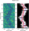 |
Fig. 1 Zoom on the track of Kepler-128 c in a river diagram with a folding period of 22.8030 days. The left panel shows the detrended data with a clipping at 3σ. The right panel shows the corresponding confidence matrix which is the output of the RIVERS.deep algorithm. Black indicates noise or missing data; white indicates the track of a planet. The track having the highest confidence is highlighted in blue. For comparison, the transit timings reported by Rowe et al. (2015) are shown in red. See Fig. 4 for further comparisons. |
2.4 Data pre-processing
For each star, the raw PDCSAP flux was downloaded using the lightkurve1 package. Long-cadence and short-cadence data were downloaded and pre-processed separately. The preprocessing steps are as follows. We started by checking for gaps longer than 2.5 h. Such gaps were commonly produced by the monthly data downlinks. After repointing the spacecraft, there was usually a photometric offset produced due to thermal changes in the telescope. We therefore removed all data points 6 h prior, and 12 h after such an interruption. We then created a copy of each light curve in which we removed in-transit data for all the known planets in the system (a window of three times the transit duration was centred on the transit timing predicted by the output of RIVERS.deep) and applied a B-spline detrending on the remaining data using keplersplinev22. We used the ‘choosekeplersplinev2’ function, forcing the timescale τ to remain larger than three times the longest transit duration of the planets in the system, with a limit of 1.5 days. The best τ (minimising the Bayesian information criterion) was then saved for use during the photo-dynamical fit (see Sect. 2.5). We then checked the mean value of the detrended light curve within a sliding window of five hours. If this mean value departs from 1 by more than once the standard deviation of the light curve for the long-cadence data (and a third of the standard deviation for the short cadence data), it implies that the local behaviour of the light curve cannot be modelled by the B-splines. In this case, we flag all data point that are within the five-hour window ±τ. We then used the raw data from which only the data near the downlinks were removed and we additionally removed the data points we flagged. This is the raw data that is used in Sect. 2.5.
2.5 Photo-dynamical fit of the light curve
The fits of the light curves were performed using a similar setup to the one presented in Leleu et al. (2021b). For each system, we used the adaptive MCMC sampler samsam3 (see Delisle et al. 2018), which learns the covariance of the target distribution from previous samples to improve the subsequent sampling efficiency. The transit timings of the planets were modelled using the TTVfast algorithm (Deck et al. 2014). The approximate initial conditions for the orbital elements and masses of these planets were obtained by a preliminary fit of the transit timings to the timing proxy obtained from the application of RIVERS.deep (Sect. 2.3, blue curve in Fig. 1). We modelled the transit of each planet with the batman package (Kreidberg 2015). For the long-cadence data, we used a supersampling parameter set to 29.42 min to account for the long exposure of the dataset. The effective temperature, log ɡ, and metallicity of the star (see Sect. 2.2) were used to compute the quadratic limb-darkening coefficients, u1 and u2, and their error bars were adapted to the Kepler spacecraft using LDCU (Deline et al. 2022). Based on the limb-darkening package (Espinoza & Jordán 2015), LDCU uses two libraries of stellar atmosphere models, ATLAS9 (Kurucz 1979) and PHOENIX (Husser et al. 2013), to compute stellar intensity profiles for a given pass-band.
We worked directly with the raw (non-normalized) fluxes obtained in Sect. 2.4 and modelled them as the product of the normalized transit model and a low-frequency component which may account for both stellar variations and instrumental systematics. This low-frequency component is modelled through a cubic B-spline (see Appendix C for more details). Our model for the raw flux, f, thus takes the following form:
 (1)
(1)
where m is the normalized transit model with parameters, 9, and b is the B-spline with parameters, η. We assumed Gaussian white noise for the measurement errors, but we quadratically added a free jitter term, σjit., to the measurements error, σi. The full set of parameters of the model is (θ, η, σjit.) and the likelihood of the model is:
 (2)
(2)
where  is the (diagonal) covariance matrix of the noise and y represents the observations. We are mostly interested here in the transit related part of the model and consider the B-spline parameters η as nuisance parameters. Thus, we analytically marginalized the likelihood over η to obtain:
 (3)
(3)
The details of this procedure which allows for very efficient evaluations of the marginal likelihood are explained in Appendix C.
2.6 Masses, eccentricities, and longitudes of periastron degeneracies
Taking Pin (resp. Pout) to be the period of the inner (resp. outer) planet, these planets are close to two-planet mean motion resonance (MMR) when Pout /Pin ~ (k + q)/k, where k and q are integers, with q as the order of the resonance. All the systems we study in this paper are close to first-order MMR (see Sect. 3.3), except Kepler-60, whose three planets are pairwise within firstorder MMRs and Kepler-26 which is near a second-order MMR (q = 2). Nesvorný & Vokrouhlický (2016) described the TTVs induced by first-order MMRs using an analytical model at first order in eccentricities, based on the 1-degree-of-freedom model proposed by Henrard & Lemaitre (1983). The changes of variables from the 4-degrees-of-freedom Hamiltonian of the two planets coplanar case to the 1-D model involves complex coordinates linked to the quantities:
 (4)
(4)
and
 (5)
(5)
where ein is the eccentricity of the inner planet, ϖin its longitude of periastron (resp. eout and ϖout for the outer planet), and f27 and f31 are functions of the Laplace coefficients that depend on k and α = ain/aout, with ain (resp. aout) as the semi-major axis of the inner planet (resp. outer) and min (resp. mout) is the mass of the inner planet (resp. outer). 𝒵 evolves during the resonant motion and is linked to the TTV signal near (Lithwick et al. 2012) or inside first-order MMRs (Nesvorný & Vokrouhlický 2016), while 𝒵2 has been shown to be a constant of motion at first order in eccentricities (Henrard & Lemaitre 1983; Nesvorný & Vokrouhlický 2016).
Hadden & Lithwick (2016) developed a model at second order in eccentricities, valid as long as the two planets are not too close to the resonance (see Nesvorný & Vokrouhlický 2016; Mardling 2022, in prep.). In this case, the TTV signal of near-resonant pair of planets can be split into three terms (Hadden & Lithwick 2016): the first term, called ‘fundamental’, which appears for pairs near first-order MMRs, is a sinusoidal signal whose frequency is associated with the super period:
 (6)
(6)
The secondary term is a sinusoid with twice this frequency, and the third term is the high-frequency 'chopping' signal. The chopping signal depends only on the masses, while the fundamental and secondary terms both depend on the masses and 𝒵 Observing only the fundamental term is thus not enough to disentangle 𝒵 from the planetary masses: the chopping signal or the secondary term have to be observed as well.
For planets closer to or inside the MMR, recovering the masses requires observing either the secondary harmonics in the amplitude of libration of the resonant angle or the observation of a second, lower frequency signal (Nesvorný & Vokrouhlický 2016; Mardling 2022, in prep.).
Good constraints on the masses hence generally translate to good constraints on the quantity 𝒵, however the constant 𝒵2 needs to be determined to access the eccentricity and longitude of the periastron of the planets. The full determination of the orbits hence requires recovering signals beyond the first order of eccentricities of the two-planet model4.
As we show in Sect. 3, in some cases, the non-fundamental harmonics can be constrained well enough to estimate 𝒵2 as well. However, when 𝒵2 remains unconstrained, the posterior of the variables (ein, ϖin, eout, ϖout) is highly degenerate. Low-eccentricity solutions in the posterior distribution tend to correspond to small values of  and anti-aligned longitudes of periastra (see Fig. 11 of Leleu et al. 2021b), while higher-eccentricity solutions tend to correspond to larger values of
  and to aligned longitudes of periastra. Such a peculiar posterior shape has also been found for resonant systems (e.g. Panichi et al. 2019; Leleu et al. 2021b, 2022). In this case, a large value of
  can lead to a precession of the longitude of the periastra of the planets, which can lead to a circulation of the resonant angles of the pair despite the fact that the orbit is formally resonant.
The dependence of the analytical TTV expression on 𝒵 only suggests that the degeneracies discussed above may be best explored via the coordinate ei cos ϖi, and ei sin ϖi (which themselves are linear combinations of the real and imaginary parts of 𝒵 and 𝒵2). Indeed, this choice produces elliptic-shaped correlations between these parameters, while others such as (ei, ϖi) or  produce contorted correlations (see Fig. 2) and may prevent our MCMC from adequately exploring the parameter space.
 |
Fig. 2 Examples of correlation between parameters of the posterior of Kepler-345 (see Sect. 3). These correlation appears when |
2.7 Priors
We used wide, flat priors for the mean longitude, period, impact parameter, jitter, and ratio of the radius of the planet over the radius of the star, Rp/R⋆. The stellar density and limb-darkening parameters have Gaussian priors. In order to test for the mass-eccentricity degeneracy inherent to pairs of planets near mean-motion resonances (Boué et al. 2012; Lithwick et al. 2012), Hadden & Lithwick (2017) fitted the transits using different priors for masses and eccentricities. Their ‘default’ prior is log-uniform in planet masses and uniform in eccentricities. Their ‘high-mass’ prior is uniform in planet masses and loguniform in eccentricities. We used the same choice of priors in order to be able to compare the posteriors of the photo-dynamical fit to their fit of pre-extracted transit timings. In addition, we performed a third fit, using log-uniform mass prior and the Kipping (2013) prior for the eccentricity: a β-distribution of parameters α = 0.697 and β = 3.27. The posterior associated with this set of prior is referred to as the ‘final’ posterior.
3 Results
The transit timings estimated for each planet, as well as 300 samples of the final posterior for each system, can be found at the CDS.
3.1 Pre-extracted transit timings or photo-dynamical analysis: Effect on the mass-radius relationship of exoplanets
In the introduction to this paper, we explain how the use of pre-extracted transit timings (e.g. Rowe et al. 2014, 2015; Holczer et al. 2016) might not be ideal when the S/N of individual transits (S/Ni, which we define as the S/N reported by the Kepler team divided by the square root of the number of transits reported by the Kepler team) is too low: adding an additional free parameter per transit might not fully recover the information from the light curve when individual transits are below the noise level. In this section, we compare the posterior of the fit of pre-extracted transit timings to the posterior of a photo-dynamical fit. For this comparison, we used the default set of priors for masses and eccentricities from Hadden & Lithwick (2017). We illustrate in Fig. 3 the difference in the posterior of the masses and radii of exoplanets depending on the use of pre-extract transit timings (see Hadden & Lithwick 2017, for the posterior of the masses and references therein for the radii) in black or photo-dynamical analysis (this paper) in green. The five most degenerate mass posteriors were removed from this plot to highlight the trend (see Table 2). The bulk of the previous radius estimates had rather large uncertainties, making it hard to distinguish a clear trend in the shift of the radius of the planets. The masses, however, shift toward a larger value as a result of the photo-dynamical analysis. The photo-dynamical posterior of Kepler-128 exhibits a shift from ~0.7 M⊕ for both planets to masses in the 3–4 M⊕ range, which is highlighted in purple in Fig. 3. Two causes were identified to explain such a difference: the pre-extracted transit timings yield lower-amplitude TTVs compared to those which are recovered with the photo-dynamical fit and the photo-dynamical fit can constrain TTVs beyond the first harmonic, allowing the mass-eccentricity degeneracy to be broken (Lithwick et al. 2012; Hadden & Lithwick 2017).
3.1.1 Amplitude of recovered TTV signals
To illustrate the effect that pre-extracting the TTVs exerts on the recovered TTV amplitude, we begin with Kepler-128 (Fig. 4). The pre-extracted transit timings are shown in black with error bars (Rowe et al. 2015), while the curves going through the bestfit TTVs of the photo-dynamical model are shown in blue. Its main frequency is extracted. Then, a linear trend and a sinusoid of that frequency is fit to the pre-extracted transit timings in red (dashed) and to the TTVs of the best fit in green (dashed). In this example, the sinusoidal approximations of the pre-extracted TTVs and of the photo-dynamical model show strong differences. The S/Ni of both planets of Kepler-128 are rather small (~2.7 and 3.1) and as a result, their pre-extracted transit timings appears to not be efficiently recovered. If we assume that the two-planet model is correct, it also appears that the error-bars of the pre-extracted transit timings are underestimated. Another system, Kepler-60 is one of the rare system known in Laplace resonance and is hence of particular interest. With three known planets with S/Nis in the range 1.68 (Kepler-60 d) to 2.41 (Kepler-60 c), we show the effect of the TTV pre-extraction in Fig. 5. While the sinusoidal approximation may be less valid in this case, the first hundred days of Kepler-60 d shows what might be the result of the initialisation for the search of TTVs: the individual transit timings are initialised on a fixed-period ephemeride, then allowed to vary. Some of the transit timings caught the real planet track (three points near −150 min of TTV), while others (three points near 0 mins of TTV) probably became trapped in a local minimum closer to 0 mins TTVs, namely, their initialisation. More generally, the pre-extracted TTVs of the three planets of Kepler-60, as in the case of the two planets of Kepler-128, shows numerous outliers, implying that the local search for each transit timings found noise structures that were preferred over the actual transit.
The effect of the S/Ni on the recovered TTV amplitude may be validated by an analysis of the whole dataset. Figure 6 shows the difference between the peak-to-peak TTV amplitude for the sinusoid approximation and the pre-extracted transit timings (in black) and photo-dynamical analysis (coloured). In all cases where S/Ni ≳ 3.5, the recovered amplitude of TTVs varies by a few minutes at most, while the amplitude can differ by several tens of minutes for lower S/Nis. This effect is further highlighted in Fig. 7. In that figure, we show the pre-extracted TTVs from Rowe et al. (2015) that are used by Hadden & Lithwick (2017). We also show the timings of Holczer et al. (2016) that were extracted by a different method. The top panel shows the difference in amplitude of the sinusoidal approximation, while the bottom panel shows the reduced chi-squared  of the published transit timings and their error with respect to the timings of our best photodynamical fit (blue curves in Figs. 4 and 5). The two databases display different behaviours: the timings from Rowe et al. (2015) appear to miss most of the large amplitude TTVs for low S/Ni, but have a relatively lower
  , while the timings from Holczer et al. (2016) appear to have a relatively better estimation of the overall TTV amplitudes, but with a relatively larger fraction of outliers (larger
  ). Interestingly, even planets with relatively high S/Ni (Kepler-176 c, S/Ni = 13.1) have a large number of outliers. These differences can be explained by their different approaches: the method of Rowe et al. (2015) is ‘local’: they first initialise the transit timings along a fixed-period ephemeride, then, if significant TTVs are observed, they update the transit shape and recompute the transit times. In some cases, they use two transit timing measurements to linearly extrapolate an estimate of the next transit time to initialize the fitter (Rowe et al. 2014). This leads to successive updates of an initially flat TTV curve. Holczer et al. (2016) conducted a broader search by systematically looking through a grid of timings around the expected transit time; hence, each transit a better chance of recovering the correct timing regardless of the other transits. At the same time, a broader search would also increase the risk of fitting background noise, which can explain the larger
  . We note that three of the smallest S/Ni values (Kepler-345 b: S Ni = 0.89, Kepler-60 b: S/Ni = 1.98, and Kepler-60 d: S/Ni = 1.68) are not included in the Holczer et al. (2016) database.
In order to recover robust planetary masses, both the main TTV amplitude and the lower amplitude-higher frequency signals are important: in the case of systems outside of MMR, the main TTV amplitude is directly linked to the estimated mass of the planets, while higher harmonics help to break the mass-eccentricity degeneracy (see Sect. 2.6).
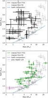 |
Fig. 3 Posteriors of the mass-radius relation for a subset of the Kepler planetary systems studied in this paper. Black bars show the radii and masses resulting from the analysis of pre-extracted transit timings (Hadden & Lithwick 2017). Green bars show the outcome of RIVERS (RIVERS.deep + the photo-dynamical fit). The priors on masses and eccentricities are set to the default prior and identical in both studies. The blue line shows the earth's composition. The position of Kepler-128 from the top panel is also shown on the bottom panel in purple, with a purple line showing its shift in the mass-radius diagram. |
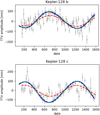 |
Fig. 4 TTVs of the near-resonant pair Kepler-128 b,c. Black bars show the pre-extracted transit timings from Rowe et al. (2015), while blue bars show the best photodynamical fit. Dashed red and green curves show sinusoidal approximations for the pre-extracted transits and the photo-dynamical analysis respectively. |
Final posterior value for 34 Kepler planets.
3.1.2 Mitigation of the mass-eccentricity degeneracy
Following Hadden & Lithwick (2017), we explored the mass-eccentricity degeneracy intrinsic to systems close to but outside MMRs (Lithwick et al. 2012). The choice of priors is detailed in Sect. 2.7. Figure 8 reports the mass posteriors of each planet resulting from the RIVERS analysis (RIVERS.deep + photo-dynamical analysis) in green and blue (this study), and the posteriors obtained by adjusting pre-extracted transit timings from Rowe et al. (2015) by Hadden & Lithwick (2016) in black and grey. The default prior tends to draw the posterior towards lower masses and larger eccentricities, while the high-mass prior draws the posterior toward larger masses. The closer these two posteriors are to one another, the less the posterior depends on the prior and the more robust the mass estimate. Figure 8 shows that the photo-dynamic analysis tends to significantly reduce the discrepancies between the posteriors, providing a more robust mass estimation. This is explained by the ability of the photo-dynamical analysis to better constrain the higher harmonics of the TTV signals (see Sect. 2.6). In addition to setting better constraints on the amplitude of the dominant harmonic of the TTVs as shown in Fig. 8, the photo-dynamical fit also better constrains the chopping or secondary term in several systems, reducing the mass-eccentricity degeneracy. Figure 9 shows the TTVs of Kepler-57, highlighting the recovery of a strong nonfundamental harmonic (see the blue curve). The relative size of the TTV harmonics, computed from the analytical model of Hadden & Lithwick (2016), are shown and discussed in Appendix B.
To provide our masses estimates, we chose to run a fit with the third set of priors, labelled as ‘final’ and shown in blue in Fig. 8, which has the same log-uniform mass prior as the Hadden & Lithwick (2017) ‘default’ prior. However, the ‘default’ prior is uniform in eccentricity. We chose the ‘final’ prior to being somewhat skewed toward lower eccentricities, as we deem it to be more realistic (see Sect. 2.7). We then quantified the degeneracy impacting each mass estimate using the quantity:
 (7)
(7)
Here,
 (8)
(8)
where mhigh,0 is the maximum of the default and high-mass posterior medians, mfinal,0 is the median of the final posterior, and mfinal,+σ is the 0.84 quantile of the final posterior, while
 (9)
(9)
where mlow,0 is the minimum of the default and high-mass posterior medians, and mfinal,-σ is the 0.16 quantile of the final posterior. We then set an arbitrary threshold of Δdegen = 1.3, below which we consider the masses to be constrained enough to be of use to the community. The masses and radii for all planets are reported in Table 2. For the planets which satisfy Δdegen ≤ 1.3, the final mass and density posterior is given. For planets where Δdegen > 1.3, an interval is given for the mass, with bounds corresponding to the lowest 0.16 and highest 0.84 quantiles of the three posteriors. The eccentricity is treated in the same way, with the definition of Δe reported in Table 2. The reported radius comes from the final posterior, although its value is always consistent across all three posteriors.
Hadden & Lithwick (2017) considered a mass estimation robust if the median of the high-mass posterior lay within the 0.16–0.84 quantile interval of the default posterior. Out of the re-analysed systems, only Kepler-26 c, Kepler-49 b and c, and Kepler-60 d were robust in their analysis (see the overlap of the black and grey errorbars in Fig. 8). For these planets, we find very similar results across all our posteriors, implying that the two-priors test proposed by Hadden & Lithwick (2017) is able to properly identify which masses are robust and which are not, regardless of the quality of the pre-extracted transit timings. In other words, poorly-determined transit timings did not ‘mimic’ strongly constrained planetary masses in their analysis.
The systems we analysed also partly overlap with those studied by Jontof-Hutter et al. (2016). To estimate the robustness of their solution, they also performed several tests including different eccentricity priors. Amongst the measurements labelled as ‘precise’ are Kepler-26, with  and
and  , and Kepler-60:
  ,
,  and
and  M⊕. These estimations are mostly 1 − σ compatible with our results presented in Table 2, except for Kepler-60 b where the difference is of ~2σ. Amongst their ‘less secure’ solutions are Kepler 57 with
  and
and  and Kepler-49 with
  and
and  M⊕. Although our result somewhat agrees for Kepler-57, we obtain a robust mass estimation that strongly disagrees with their solution for Kepler-49. Our results hence also agree with the robustness tests of Jontof-Hutter et al. (2016).
From this analysis, we have drawn two main conclusions: (1) tests such as those presented in Hadden & Lithwick (2017), Jontof-Hutter et al. (2016) or this paper are necessary to ensure the robustness of TTV-characterised masses and (2) the recovery of the TTV signal (here using RIVERS.deep) and the photo-dynamical fit of the light curve can significantly increase the robustness of mass estimations.
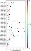 |
Fig. 6 Peak-to-peak TTV amplitudes of the sinusoidal approximation of all of the planets that were analysed in this study. Black points are fits to the pre-extracted timings published by Rowe et al. (2015), which for Kepler-128 and Kepler-60 correspond to the red-dashed curves in Figs. 4 and 5. The coloured diamonds show the peak-to-peak amplitude of the sinusoidal approximation of the best fit of the photo-dynamical model (the green dashed curves in Figs. 4 and 5). The colour indicates the S/Ni of the planet. The agreement between pre-extracted timings and photo-dynamical fit is reduced for lower S/Ni. This is further highlighted in Fig. 7. |
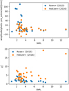 |
Fig. 7 Difference between the amplitude of the sinusoidal approximation of both the best solution of the photo-dynamical analysis and pre-extracted transit timings (top). The blue dots correspond to the timings from Rowe et al. (2015), and in orange from Holczer et al. (2016). Reduced chi-squared between the published transit timings and the best solution of the photo-dynamical fit (bottom). |
3.1.3 Addition of a third planet
Here, we discuss the example of Kepler-24 with four known planets. Hadden & Lithwick (2017) only considered Kepler-24 b and c at 8 14 and 12 33 day. The inner planet at 4 24 day is too far from any significant MMR with the other planets to have significant TTVs. Kepler-24 e, however, with an orbital period of 19.00 days, has a period ratio of ~1.54 with Kepler-24 c. Due to its small S/Ni (≈1.8), no clear TTV signal is recognisable in the pre-extracted transit timings (see the top panel of Fig. 10). However, using RIVERS, we were able to recover TTVs of ~50 min of peak-to-peak amplitude. The bottom panel of Fig. 10 show the difference in the mass determination of Kepler-24 between the two- and three-planet model. In the three-planet model, Kepler-24 e is unconstrained, but its TTVs help to break the degeneracy on the inner part of the system. A similar test was performed for Kepler-23: the addition of Kepler-23 d helped to better constrain the whole system, also shifting the masses of Kepler-23 b and Kepler-23 c toward larger values, while remaining consistent within 1–2σ with the two-planet solution.
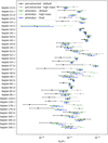 |
Fig. 8 In black and grey, the default and high-mass posteriors of the fit of pre-extracted TTVs from Rowe et al. (2015) by Hadden & Lithwick (2017). In green and blue, we give the posteriors from the RIVERS analysis. Dark green shows the default posterior, light green the high-mass posterior, and blue the final posterior. The full photo-dynamical analysis reduces the prior dependency, thereby increasing massestimate robustness, for most planets of the sample. |
3.2 Masses, radii, and densities
Here we compare the mass-radius relationship of the sample of re-analysed Kepler planets to the samples of exoplanets for which the mass was estimated by the radial-velocity technique. We use the DACE database5 (Otegi et al. 2020) and select only the planets for which the mass uncertainty is below 50% and the radius uncertainty below 30%. The mass-radius measurements of this population is shown in grey in Fig. 11. The figure shows the posterior of the final photo-dynamical fit, with the mass degeneracy indicator, ΔM, colour-coded. The mass-radius measurements are also compared to various theoretical mass-radius relationships in Fig. 12. This includes (1) pure solid interiors (pure iron, terrestrial Earth-like, pure MgSiO3 rocky), taken from Zeng et al. (2016); (2) terrestrial interiors with H2/He envelopes, taken from Zeng et al. (2019); (3) terrestrial interiors with H2O steam envelopes, taken from Aguichine et al. (2021). The steam mass-radius relationships are the most appropriate here for water (with respect to liquid and icy interiors) given all planets of the sample are more irradiated than the runaway greenhouse limit (Turbet et al. 2020). Mass-radius relationships with H2 and H2O envelopes are arbitrarily plotted for various temperatures (500 K, 700 K, 1000 K; from the smallest to the largest radius) which are representative of the equilibrium temperatures of our sample of planets.
Firstly, we notice in Fig. 11 that the low-mass-and-large-radius population amongst the re-analysed planets (Kepler-24 e, Kepler-176 c and d) is not, in fact, robust. This is a reassuring result, as these planets should theoretically not be able to maintain a stable hydrogen envelope, given their low mass and the high irradiation they receive. These planets are indeed located in the part of the mass-radius diagram where the radius of a H2-rich planet increases as the mass of the planet decreases (see Fig. 12). This is symptomatic of the fact that the gravity of the planet is insufficient to guarantee the hydrostatic equilibrium of a H2/He envelope.
Secondly, we notice that the robust TTV-characterized planets (in this work) exhibit a tendency toward a lower density than the RV-characterised planets, in particular, the cluster of planets of masses between 2 and 3 M⊕ and radius below 2 R⊕. Most of the TTV-characterized planets lie above the pure rock (100% MgSiO3, black curve in Fig. 12), indicating that they must have a H2-rich or a volatile (e.g. water) envelope (Zeng et al. 2019; Bean et al. 2021). The mass-radius relationships alone do not lift the degeneracy between either of these two scenarios, at least for most planets of our sample. It is still not clear whether the tendency toward lower density of TTV planets (compared to RV planets) is due to the sensibility of the RV method toward more massive planets (RV planets for which the mass is known with better than 50% are plotted in Figs. 11 and 12, while low-mass planet have a tendency of having a lower precision on their mass) or if, in fact, it testifies to their distinct formation and evolution histories. We notice that the TTV planets have on average a lower equilibrium temperature than RV planets (Teq = 768 ± 246K for the TTVs samples and 1193 ± 616K for the RV sample), which could favor the stability of H2 or H2O envelopes, and thus increase the share of planets present in the large-radius peak of the so-called radius gap (Fulton et al. 2017). This is particularly relevant for the cluster of TTV planets near 2–3 M⊕ which have moderate equilibrium temperatures.
To quantitatively explore the differences in composition between the RV and TTV planet populations, we used a Bayesian inference method to characterise further the gas mass fraction of both populations. We hypothesize for this calculation that it is the gas envelope (H2/He) that drives the observed variations in density between the planets. The full model is described in detail in (Leleu et al. 2021a) and based on (Dorn et al. 2017). More details on the method are given in Appendix D.
The results from our analysis are shown in Fig. 13. It shows (Fig. 13, left panel) the gas mass fraction (more precisely the median of the posterior distribution of the gas mass fraction as derived from the Bayesian analysis) of the modelled planets from both samples in relation to their position in a radius and equilibrium temperature diagram. In general, for both populations, the larger the radius, the larger the median of the gas mass fraction. However, for equilibrium temperatures smaller than 1000 K and radii between 1.5 and 2.5 R⊕, the re-analysed set of Kepler planets shows, on average, a much higher gas content. Indeed, the majority of RV-characterised planets have a gas mass fraction smaller than 10−6, whereas we see a significant fraction of Kepler planets with a gas mass fraction as large as 10−4. The same can be observed when looking at the corresponding mass and equilibrium temperature diagram (Fig. 13, right panel) for masses below 3 M⊕. This suggests that the equilibrium temperature difference between the RV and TTV planets alone cannot explain the differences in the gas content.
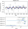 |
Fig. 10 TTVs of Kepler-24 e at the top. Details are the same as in Fig. 4. Bottom panel shows the mass posteriors of the planets of Kepler-24, depending on the addition of Kepler-24 e to the model; see Fig. 8 for a description. Adding Kepler-24 e helps to better constrain the masses of Kepler-24 b and Kepler-24 c, despite having a highly degenerate mass itself. |
3.3 Eccentricities and resonant states
The architecture of (nearly) resonant systems contains information on their formation and evolution, such as migration in the proto-planetary disc (e.g. Nesvorny et al. 2022) and tidal evolution (e.g. Lee et al. 2013). Table 3 indicates the value of the parameter Γ′ for each pair of planets. Γ′ is the parameter of the one degree of freedom model of the first order MMRs, which describes the position of a pair of planets with respect to the closest first-order MMR6 (Henrard & Lemaitre 1983; Deck et al. 2013). The power of this 1-degree of freedom model is that it allows comparing pairs of planets of different orbital periods and masses with respect to any of the first order MMRs. The resonance formally appears for Γ′≥1.5. Hence, if Γ′< 1.5, the pair cannot be resonant (although its resonant angles can librate around a given value), and Γ′ gives an estimate of the distance to the resonance. For Γ′ > 1.5, an additional test is required to check if the system lies inside the resonance, which we will not describe here. For resonant systems, Γ′ describes how ‘deep’ the pair is in the MMR. Breaking the degeneracy between the masses of the planets and 𝒵 hence does not only provide good mass estimates for the planets involved, but can also provide valuable information about their resonant state, which can in turn be linked to their proto-planetary disc or the inner planet’s internal structure. Out of all the pairs studied, only Kepler-60 b and c and Kepler-60 c and d are inside the 2-body MMRs, forming a Laplace resonant chain (Goździewski et al. 2016). We obtained good constraints on Γ′ for several of the pairs; the implications for the dissipative evolution of these systems will be the subject of a future study. Systems with large uncertainties on F, such as Kepler-128, were checked to see that they have all of their posterior outside of the resonance.
We obtain robust eccentricity estimates for 19 planets. Often the errors remain quite large, with medians of a few percent and uncertainties of similar amplitude. However some eccentricities are different from zero at more than 80-, such as Kepler-57 b and c and Kepler-60 c (see Table 2). This implies that we were able to constrain the TTVs beyond the effects of first-order in eccentricities (see Sect. 3.1.2). This results in good constraints on 𝒵2(see Table 3).
 |
Fig. 11 Mass-radius relationship of the re-analysed set of Kepler planets with the final posterior. The colour shows the degeneracy metric defined above Eq. (7): black-purple corresponds to well-constrained masses (low prior dependency), while red-yellow shows poorly constrained masses (high prior dependency). The grey background is the mass-radius relationship from RV-estimated masses. |
 |
Fig. 12 Mass-radius relationship of the robust set of Kepler planets. The colour code shows the equilibrium temperature of the planet, taken from the exoplanet archive (computed assuming a bond albedo of 0.3). |
 |
Fig. 13 Radius (left) and mass (right) as function of equilibrium temperature of both the re-analysed set of Kepler planets (larger circles with green outline) and the RV-characterised planets. Colour code shows the modelled gas mass fraction of the planets in a logarithmic scale. |
Dynamical state of 19 Kepler pairs.
4 Summary and conclusion
We re-analysed a sample of 34 Kepler planets in the super-Earth to mini-Neptune range in 15 multi-planetary systems. Most of these planets were known to have TTVs, with transit timings available in current databases Rowe et al. (2015); Holczer et al. (2016). These systems were previously characterised by fitting these pre-extracted transit timings (e.g. Jontof-Hutter et al. 2016; Hadden & Lithwick 2017). Our analysis used the RIVERS method, which first estimates the transit timings of the planets using the RIVERS.deep algorithm (CNN-based image recognition; see Sect. 2.3), then uses a photo-dynamical fit of the light curve (see Sect. 2.5).
Firstly, we showed that the transit timings resulting from our analysis often differ by several tens of percent in amplitude from the published values, introducing a systematic bias in estimates of the associated planet masses. We have shown that the amplitude of this difference is strongly anti-correlated with the signal-to-noise ratio (S/N) of individual transits of the planets, indicating that the classical approach of fitting the lightcurve, with individual transit timings as free parameters to recover the TTVs, gives poor results when the individual transit S/N is below ~4.
Secondly, using the default prior identical to the one used by Hadden & Lithwick (2017), we consistently recovered masses that were higher than those obtained by fitting pre-extracted transit timings. This difference, which can be more than 4σ as in the case of Kepler-128 (Hadden & Lithwick 2016), is explained not only by the difference in TTV amplitude, but also by the capacity of the photo-dynamic analysis to recover additional harmonics (especially when short-cadence data is available), allowing us to break the mass-eccentricity degeneracy inherent to nearly resonant pairs of planets. For the three-planet systems Kepler-23 and Kepler 24, we also tried fitting only two planets; in both cases, the three-planet study yielded larger and better constrained masses for the two planets that were present in both analyses. This highlights the model dependency inherent to the TTV method, and imply that non-transiting planets can also be responsible for underestimations of the masses of planets.
Out of the 34 planets analysed, we robustly determined the mass of 23 planets (low prior dependency; see the robustness criterion described in Sect. 3.1.2), 13 of which have a precision on the mass better than 20%. Comparing the newly-characterised planets to the RV-characterised population from (Otegi et al. 2020), it appears that some of the TTV-characterised planets still have a lower density than their RV counterparts, which is in agreement with the robustly-characterised samples of Hadden & Lithwick (2017). In terms of internal structure, this lower density translates to a larger mass fraction of gas, as derived from internal structure modeling. Although the TTV-characterized planets we study here have, on average, a lower equilibrium temperature than RV-characterized planets (which would help stabilize a gas or volatile envelope), we notice that this property alone cannot explain the observed differences in density. The difference could be due to the bias inherent to the method used to obtain the mass: higher masses make a planet easier to adequately characterise using RVs, while deeper transits allow for better transit timing estimates. Another explanation could be related to the fact that planetary systems characterised by TTVs are necessarily compact multi-planetary systems. The difference in density could therefore be related to the formation and evolution history of the systems. More studies, comparing larger samples and correcting the effect of observational biases, are required in order to decipher the origin of the differences between the two populations. We also leave to a future study the re-analysis of super-puff planets such as Kepler-79 (Jontof-Hutter et al. 2014), found not robust by Hadden & Lithwick (2017); and Kepler-51 (Masuda 2014; Libby-Roberts et al. 2020), found robust by Hadden & Lithwick (2017).
We constrained the eccentricities of most planets to a few percent at most, with errors on the same order. The exceptions were Kepler-57 b and c and Kepler-60 c, for which the analysis provided relatively precise estimates of the individual eccentricities, which in itself is of particular interest given that it requires adequate power in the non-dominant harmonics and because it is especially difficult to measure such small eccentricities with radial velocities. Breaking the mass-eccentricity degeneracy has also often allowed us to have a better view on the resonant state of the systems. For systems whose inner planet is far-enough from the star (typically >10 days), this will allow us to constrain the local shape of the proto-planetary disc prior to its dispersal (e.g. Nesvorny et al. 2022). For systems whose inner planet is closer to the star, the observed resonant state can allow us to constrain the tidal dissipation in the inner planets (e.g. Lee et al. 2013).
Finally, we want to stress that all of the robustly characterised planets in this study occupy a ‘believable’ position in the massradius diagram, while a single analysis of pre-extracted transit timings would often have resulted in a strong underestimation of the planetary masses. Since the quality of pre-extracted transit timings is strongly correlated with the transit S/N (hence, the planetary radius), this bias mostly affects systems of small (typically sub-Neptune) planets, which can impede the characterisation of these systems in the Kepler, TESS, and upcoming PLATO data.
Our results, combined with those of Hadden & Lithwick (2017), strongly advocate the use of several priors to explore the mass-eccentricity degeneracy, as well as the systematic use of photo-dynamical analysis to recover higher small-amplitude harmonics of the TTVs signals. Since the long baselines of the Kepler data, near-polar observations of TESS and PLATO allow for the detection of planets whose individual transits are below the noise level, recovering individual transits to initialise the photo-dynamical fit might be challenging. In this case, we have shown that the use of RIVERS.deep, based on the the recognition of the track of a planet in a river diagram using a neural network, could recover the transit timings of such planets.
Acknowledgements
This work has been carried out within the framework of the National Centre of Competence in Research PlanetS supported by the Swiss National Science Foundation and benefited from the seed-funding program of the Technology Platform of PlanetS. The authors acknowledge the financial support of the SNSF.
Appendix A Eccentricity and longitude of periastron posterior shapes
Figure A.1 shows the correlation between parameters for various choices of coordinates.
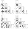 |
Fig. A.1 Corner plots of the eccentricities and longitudes of periastron of the default posterior of Kepler-345 b and c. The top-left corner shows the real and imaginary part of 𝒵 and 𝒵2, top-right corner shows the ki = ei cos ϖi and hi = ei sin ϖi variables, bottom left corner shows the ei and ϖi variables, and the bottom right corner shows the |
Appendix B Analytical modeling of TTVs
TTV amplitude of 19 Kepler pairs
Table B.1 shows the peak-to-peak amplitude of the sinusoidal approximation of the best fit of the photo-dynamical model (Sect. 3.1.1). The table also shows the different TTVs contributions from the analytical model of Hadden & Lithwick (2016), valid outside first- or second-order MMRs. These coefficients are computed as follows: we randomly selected 400 samples of the final posterior. For each of these initial conditions, we computed the analytical TTVs for each subsequent pair of planets. We computed the fundamental, secondary, and chopping signal separately based on Appendix B of Hadden & Lithwick (2016) (see Sect. 2.6 for a discussion on these terms). For the chopping signal, we computed the first ten terms of the series based on Eqs. (39) and (54) of (Hadden & Lithwick 2016). Then, for the fundamental, secondary, and the sum of the chopping terms, we computed the amplitudes by subtracting their minimum value from their maximum value over the duration of the Kepler mission. This resulted in 400 estimations of amplitude for each term. In the table, we display the median and .16 and .84 quantiles error for each amplitude across these 400 samples.
We do not display the results for Kepler-60, since the planets are inside the MMRs and therefore the model is not valid. We also note that the model does not work properly for Kepler-57, which might be strongly affected by the proximity of the resonance or require the consideration of additional terms in eccentricity. For all other pairs, the amplitude of the sinusoidal approximation is similar to the estimated amplitude of the fundamental harmonic. The table gives an idea of the relative size of the secondary and chopping terms that need to be constrained in order to break the mass-eccentricity degeneracy. However, the interpretation of these results is not straightforward. Firstly, the difficulty in detecting a harmonic depend not only on its amplitude but also strongly on the S/Ni of the planet and the availability of short cadence data. Secondly, the analytical TTV model was not directly fit to the data: small errors on secondary and chopping signals do not necessarily imply that we were able to measure these contributions with high precision, but that the overall constraints we got on the system allowed to give a precise estimation of what should be the amplitude of these terms. For example, the small uncertainties on the chopping terms of Kepler-57 illustrate this point. Thirdly, the model only considers a pair of planets.
Appendix C B-splines and marginalization of the likelihood
In this appendix, we describe the B-spline model used to account for stellar variations and instrumental systematics, as well as the method we use to efficiently compute the likelihood marginalized over the B-spline parameters. A cubic B-spline is a piecewise third order polynomial that is twice as continuously differentiable everywhere. We assume here regularly spaced knots and denote, using τ, the time lag between two knots. The value of τ is chosen in order to avoid over-fitting short term variations associated with the transits but still model as much as possible of stellar variations and instrumental systematics. The procedure used to select the value of τ is described in Sect. 2.4. For a time series with large interruptions (Δt > 4τ), the B-splines over each of the segments of continuous observations are independent from each other. Thus, the full marginal likelihood is simply the product of the marginal likelihoods over each segment. We thus consider here a single segment with continuous observations (Δt < 4τ). For a segment with time span T, we have N = [T/τ] pieces (N + 1 knots). We centre the time series in the sense that we set the positions (τk) of the knots such that the lag between the first knot and the first measurement (t1 − τ1) is the same as the lag between the last measurement and the last knot (τN+1−tn). The B-spline is defined as a linear combination of N + 3 splines. Each piece is modeled as a combination of four splines and, reciprocally, each spline is defined over four consecutive pieces (except on the edges). The parameters η of the model are the N + 3 coefficients appearing in the linear combination of the splines. For t ϵ [τk,τk+1], we have:
 (C.1)
(C.1)
where δ = t − τk. The time series b(η, t) thus takes the form:
 (C.2)
(C.2)
where B is the (n × (N + 3)) matrix defined as
 (C.3)
(C.3)
with nk the index of the last measurement that lies in the range [τk,τk+1] and
 (C.4)
(C.4)
The matrix B can thus be stored in an efficient manner in the form of the (n × 4) matrix β.
We now aim at computing the marginal likelihood of Eq. (3). For this purpose, we first need to set a prior on the parameters η. We assume for η a centred Gaussian prior with covariance Λ, which is independent of the other parameters (θ, σjit.)
 (C.5)
(C.5)
We additionally assume Λ to be diagonal in the following. For a given set of parameters θ, we can compute the transit model m(θ, t), and define
 (C.6)
(C.6)
where * denotes the Hadamard (element-wise) product of each column of B by the vector m. The matrix A possesses the exact same structure as B and can be stored using the n × 4 matrix a = m * β. The marginal likelihood of Eq. (3) can then be rewritten as
 (C.7)
(C.7)

which can be integrated as
 (C.8)
(C.8)
with
 (C.9)
(C.9)
This expression could be further simplified using the Woodbury identity to obtain a simple Gaussian distribution for y (e.g. Luger et al. 2017):
 (C.10)
where
 (C.11)
However, while this latter expression is more compact, evaluating the marginal likelihood using it requires to compute the determinant of S and to solve for yTS−1y, with S a (n × n) matrix. Thus, the cost of a likelihood evaluation typically scales as O(n3). For Σ and A diagonal, the matrix S is actually banded with bandwidth w = maxk(nk+3 − nk−1). This structure might allow us to improve performances (scaling in O(w2n)), but since the number of measurements is usually much larger than the number of pieces (n » N), the bandwidth w is still a large fraction of n. In such a case, a more efficient method is to keep the marginal likelihood in the form of Eq. (C.8). Indeed, for Σ and A diagonal, C−1 is a symmetric banded matrix with bandwidth 3, and the cost of likelihood evaluations can be reduced to 𝒪(n). We first define
 (C.12)
with  . With these new notations, we have
 (C.13)
We additionally introduce the piecewise notations
 (C.14)
and for each piece we compute the (4 × 4) matrix:
 (C.15)
and the vector of size 4,
 (C.16)
We then obtain the lower banded representation of the matrix GTG with
 (C.17)
and the vector x with
 (C.18)
for i ϵ [1, N + 3] and d ϵ [0,3]. Since A is assumed to be diagonal, the lower banded representation of C−1 is straightforward to compute from Eq. (C.17). Finally, we compute the Cholesky decomposition C−1 = LLT in lower banded form which allows to straightforwardly compute the determinant of C and to solve for xTCx = (L−1 x)T(L−1 x). Using algorithms dedicated to banded matrices, both the Cholesky decomposition and the solving have a computational cost scaling as 𝒪(n).
In practical computations, we assume that the priors on the B-spline parameters η are sufficiently broad (i.e. the diagonal entries of Λ are sufficiently large) such that C−1 ≈ GTG. Moreover, we additionally ignore the determinant of A in Eq. (C.8) since it is a constant renormalization factor which does not have any impact in our analyses. These approximations are equivalent to assuming a uniform prior for the parameters η with unspecified very large bounds.
Appendix D Internal structure model
For both the sample of re-analysed Kepler planets and the sample of RV-characterised planets, we used a Bayesian inference method to characterise the internal structure of the planets. The full model is described in detail in (Leleu et al. 2021a) and based on (Dorn et al. 2017).
We assume that the planets are spherically symmetric and consist of four fully differentiated layers (iron core, silicate mantle, water, and H/He atmosphere). In terms of equations of state, we use Hakim et al. (2018) for the iron core, Sotin et al. (2007) for the silicate mantle, and Haldemann et al. (2020) for the water layer, along with the atmosphere model of Lopez & Fortney (2014). We further assume that the H/He atmosphere is independent of the rest of the planet and fix the temperature and pressure at the gas-water boundary. We thereby neglect effects of the gas layer on the solid part of the planet, such as atmospheric pressure or thermal insulation.
In the sample of RV-characterised planets, for many planets, at least some of the stellar observables are unknown. Therefore, we limit the stellar input parameters of the Bayesian model to the observables that are known for all planets from both samples: mass, radius, and the effective temperature of the star. For these values, we assume an error of 5%, since reliable error bars are not generally available. Furthermore, we assume the stars to be of Solar composition, also within error bars of 5%. For the age of the stars, we assume it is unconstrained (5 ± 5 Gyr). The planetary input parameters of the model are the mass and radius values with the respective errors and the period with an assumed error of 0.1%. Additionally, the model assumes that the composition of the modelled planet matches the one of the star exactly (see (Thiabaud et al. 2015)). We note that the evidence for this is not quite conclusive; in addition, Adibekyan et al. (2021) recently showed that the correlation might in fact not be a 1:1 relationship.
We stress that the results from the Bayesian inference model depend to some extent on the chosen priors and would differ if very different priors were chosen. Again following the method detailed in (Leleu et al. 2021a), we assume a log-uniform prior for the gas mass and a prior that is uniform on the simplex for the iron core, mantle, and water mass fractions with respect to the solid planet. However, we assume we choose an upper limit of 50% for the water mass fraction (see (Thiabaud et al. 2014) and (Marboeuf et al. 2014)). The results from our analysis are shown in Figure 13.
References
- Adibekyan, V., Dorn, C., Sousa, S. G., et al. 2021, Science, 374, 330 [NASA ADS] [CrossRef] [Google Scholar]
- Agol, E., & Deck, K. 2016, ApJ, 818, 177 [Google Scholar]
- Agol, E., Steffen, J., Sari, R., & Clarkson, W. 2005, MNRAS, 359, 567 [Google Scholar]
- Agol, E., Dorn, C., Grimm, S. L., et al. 2021, Planet. Sci. J., 2, 1 [NASA ADS] [CrossRef] [Google Scholar]
- Aguichine, A., Mousis, O., Deleuil, M., & Marcq, E. 2021, ApJ, 914, 84 [NASA ADS] [CrossRef] [Google Scholar]
- Alibert, Y., Carron, F., Fortier, A., et al. 2013, A&A, 558, A109 [NASA ADS] [CrossRef] [EDP Sciences] [Google Scholar]
- Almenara, J. M., Díaz, R. F., Dorn, C., Bonfils, X., & Udry, S. 2018, MNRAS, 478, 460 [CrossRef] [Google Scholar]
- Auclair-Desrotour, P., Laskar, J., Mathis, S., & Correia, A. C. M. 2017, A&A, 603, A108 [NASA ADS] [CrossRef] [EDP Sciences] [Google Scholar]
- Batygin, K., & Morbidelli, A. 2013, A&A, 556, A28 [NASA ADS] [CrossRef] [EDP Sciences] [Google Scholar]
- Bean, J. L., Raymond, S. N., & Owen, J. E. 2021, J. Geophys. Res. Planets, 126, e06639 [NASA ADS] [CrossRef] [Google Scholar]
- Berger, T. A., Huber, D., van Saders, J. L., et al. 2020, AJ, 159, 280 [Google Scholar]
- Boué, G., Oshagh, M., Montalto, M., & Santos, N. C. 2012, MNRAS, 422, L57 [NASA ADS] [Google Scholar]
- Carter, J. A., Agol, E., Chaplin, W. J., et al. 2012, Science, 337, 556 [Google Scholar]
- Coleman, G. A. L., Leleu, A., Alibert, Y., & Benz, W. 2019, A&A, 631, A7 [NASA ADS] [CrossRef] [EDP Sciences] [Google Scholar]
- Cubillos, P., Erkaev, N. V., Juvan, I., et al. 2017, MNRAS, 466, 1868 [Google Scholar]
- Deck, K. M., Payne, M., & Holman, M. J. 2013, ApJ, 774, 129 [Google Scholar]
- Deck, K. M., Agol, E., Holman, M. J., & Nesvorný, D. 2014, ApJ, 787, 132 [CrossRef] [Google Scholar]
- Deline, A., Hooton, M. J., Lendl, M., et al. 2022, A&A, 659, A74 [NASA ADS] [CrossRef] [EDP Sciences] [Google Scholar]
- Delisle, J.-B. 2017, A&A, 605, A96 [NASA ADS] [CrossRef] [EDP Sciences] [Google Scholar]
- Delisle, J.-B., Correia, A. C. M., Leleu, A., & Robutel, P. 2017, A&A, 605, A37 [NASA ADS] [CrossRef] [EDP Sciences] [Google Scholar]
- Delisle, J.-B., Ségransan, D., Dumusque, X., et al. 2018, A&A, 614, A133 [NASA ADS] [CrossRef] [EDP Sciences] [Google Scholar]
- Dobrovolskis, A. R., & Borucki, W. J. 1996, BAAS, 28, 1112 [NASA ADS] [Google Scholar]
- Dorn, C., Venturini, J., Khan, A., et al. 2017, A&A, 597, A37 [NASA ADS] [CrossRef] [EDP Sciences] [Google Scholar]
- Emsenhuber, A., Mordasini, C., Burn, R., et al. 2021, A&A, 656, A69 [NASA ADS] [CrossRef] [EDP Sciences] [Google Scholar]
- Espinoza, N., & Jordán, A. 2015, MNRAS, 450, 1879 [Google Scholar]
- Fulton, B. J., Petigura, E. A., Howard, A. W., et al. 2017, AJ, 154, 109 [Google Scholar]
- García-Melendo, E., & López-Morales, M. 2011, MNRAS, 417, L16 [NASA ADS] [Google Scholar]
- Gozdziewski, K., Migaszewski, C., Panichi, F., & Szuszkiewicz, E. 2016, MNRAS, 455, L104 [Google Scholar]
- Grimm, S. L., Demory, B.-O., Gillon, M., et al. 2018, A&A, 613, A68 [NASA ADS] [CrossRef] [EDP Sciences] [Google Scholar]
- Hadden, S., & Lithwick, Y. 2016, ApJ, 828, 44 [NASA ADS] [CrossRef] [Google Scholar]
- Hadden, S., & Lithwick, Y. 2017, AJ, 154, 5 [Google Scholar]
- Hakim, K., Rivoldini, A., Van Hoolst, T., et al. 2018, Icarus, 313, 61 [Google Scholar]
- Haldemann, J., Alibert, Y., Mordasini, C., & Benz, W. 2020, A&A, 643, A105 [NASA ADS] [CrossRef] [EDP Sciences] [Google Scholar]
- Henrard, J., & Lemaitre, A. 1983, Celest. Mech., 30, 197 [Google Scholar]
- Holczer, T., Mazeh, T., Nachmani, G., et al. 2016, ApJS, 225, 9 [Google Scholar]
- Huber, D., Chaplin, W. J., Christensen-Dalsgaard, J., et al. 2013, ApJ, 767, 127 [Google Scholar]
- Husser, T. O., Wende-von Berg, S., Dreizler, S., et al. 2013, A&A, 553, A6 [NASA ADS] [CrossRef] [EDP Sciences] [Google Scholar]
- Jégou, S., Drozdzal, M., Vazquez, D., Romero, A., & Bengio, Y. 2017, in Proceedings of the IEEE Conference on Computer Vision and Pattern Recognition (CVPR) Workshops, 11 [Google Scholar]
- Jenkins, J. M., Caldwell, D. A., Chandrasekaran, H., et al. 2010, ApJ, 713, L87 [Google Scholar]
- Jenkins, J. M., Twicken, J. D., McCauliff, S., et al. 2016, Proc. SPIE, 9913, 99133E [Google Scholar]
- Jontof-Hutter, D., Lissauer, J. J., Rowe, J. F., & Fabrycky, D. C. 2014, ApJ, 785, 15 [NASA ADS] [CrossRef] [Google Scholar]
- Jontof-Hutter, D., Ford, E. B., Rowe, J. F., et al. 2016, ApJ, 820, 39 [Google Scholar]
- Kane, M., Ragozzine, D., Flowers, X., et al. 2019, AJ, 157, 171 [NASA ADS] [CrossRef] [Google Scholar]
- Kipping, D. M. 2013, MNRAS, 434, L51 [Google Scholar]
- Kovács, G., Zucker, S., & Mazeh, T. 2002, A&A, 391, 369 [Google Scholar]
- Kreidberg, L. 2015, PASP, 127, 1161 [Google Scholar]
- Kurucz, R. L. 1979, ApJS, 40, 1 [NASA ADS] [CrossRef] [Google Scholar]
- Leconte, J., Wu, H., Menou, K., & Murray, N. 2015, Science, 347, 632 [NASA ADS] [CrossRef] [Google Scholar]
- Lee, M. H., Fabrycky, D., & Lin, D. N. C. 2013, ApJ, 774, 52 [NASA ADS] [CrossRef] [Google Scholar]
- Leleu, A., Alibert, Y., Hara, N. C., et al. 2021a, A&A, 649, A26 [NASA ADS] [CrossRef] [EDP Sciences] [Google Scholar]
- Leleu, A., Chatel, G., Udry, S., et al. 2021b, A&A, 655, A66 [CrossRef] [Google Scholar]
- Leleu, A., Delisle, J. B., Mardling, R., et al. 2022, A&A, 661, A141 [NASA ADS] [CrossRef] [EDP Sciences] [Google Scholar]
- Libby-Roberts, J. E., Berta-Thompson, Z. K., Désert, J.-M., et al. 2020, AJ, 159, 57 [Google Scholar]
- Lithwick, Y., Xie, J., & Wu, Y. 2012, ApJ, 761, 122 [Google Scholar]
- Lopez, E. D., & Fortney, J. J. 2014, ApJ, 792, 1 [Google Scholar]
- Luger, R., Foreman-Mackey, D., & Hogg, D. W. 2017, Res. Notes Am. Astron. Soc., 1, 7 [Google Scholar]
- Marboeuf, U., Thiabaud, A., Alibert, Y., Cabral, N., & Benz, W. 2014, A&A, 570, A36 [NASA ADS] [CrossRef] [EDP Sciences] [Google Scholar]
- Masuda, K. 2014, ApJ, 783, 53 [Google Scholar]
- Mazeh, T., Nachmani, G., Holczer, T., et al. 2013, ApJS, 208, 16 [Google Scholar]
- Mills, S. M., & Fabrycky, D. C. 2017, ApJ, 838, L11 [Google Scholar]
- Mills, S. M., & Mazeh, T. 2017, ApJ, 839, L8 [Google Scholar]
- Mills, S. M., Fabrycky, D. C., Migaszewski, C., et al. 2016, Nature, 533, 509 [Google Scholar]
- Mordasini, C. 2018, Planetary Population Synthesis (Berlin: Springer), 143 [Google Scholar]
- Mordasini, C., Alibert, Y., Benz, W., & Naef, D. 2009, A&A, 501, 1161 [NASA ADS] [CrossRef] [EDP Sciences] [Google Scholar]
- Nesvorný, D., & Vokrouhlický, D. 2014, ApJ, 790, 58 [CrossRef] [Google Scholar]
- Nesvorný, D., & Vokrouhlický, D. 2016, ApJ, 823, 72 [Google Scholar]
- Nesvorný, D., Kipping, D., Terrell, D., et al. 2013, ApJ, 777, 3 [CrossRef] [Google Scholar]
- Nesvorny, D., Chrenko, O., & Flock, M. 2022, ApJ, 925, 38 [NASA ADS] [CrossRef] [Google Scholar]
- Otegi, J. F., Bouchy, F., & Helled, R. 2020, A&A, 634, A43 [NASA ADS] [CrossRef] [EDP Sciences] [Google Scholar]
- Panichi, F., Migaszewski, C., & Gozdziewski, K. 2019, MNRAS, 485, 4601 [NASA ADS] [CrossRef] [Google Scholar]
- Ragozzine, D., & Holman, M. J. 2010, ArXiv e-prints [arXiv: 1006.3727] [Google Scholar]
- Rowe, J. F., & Thompson, S. E. 2015, ArXiv e-prints [arXiv: 1504.00707] [Google Scholar]
- Rowe, J. F., Bryson, S. T., Marcy, G. W., et al. 2014, ApJ, 784, 45 [Google Scholar]
- Rowe, J. F., Coughlin, J. L., Antoci, V., et al. 2015, ApJS, 217, 16 [NASA ADS] [CrossRef] [Google Scholar]
- Sotin, C., Grasset, O., & Mocquet, A. 2007, Icarus, 191, 337 [Google Scholar]
- Thiabaud, A., Marboeuf, U., Alibert, Y., et al. 2014, A&A, 562, A27 [NASA ADS] [CrossRef] [EDP Sciences] [Google Scholar]
- Thiabaud, A., Marboeuf, U., Alibert, Y., Leya, I., & Mezger, K. 2015, A&A, 580, A30 [NASA ADS] [CrossRef] [EDP Sciences] [Google Scholar]
- Turbet, M., Bolmont, E., Ehrenreich, D., et al. 2020, A&A, 638, A41 [NASA ADS] [CrossRef] [EDP Sciences] [Google Scholar]
- Vissapragada, S., Jontof-Hutter, D., Shporer, A., et al. 2020, AJ, 159, 108 [NASA ADS] [CrossRef] [Google Scholar]
- Weiss, L. M., & Marcy, G. W. 2014, ApJ, 783, L6 [Google Scholar]
- Wu, Y., & Lithwick, Y. 2013, ApJ, 772, 74 [Google Scholar]
- Xie, J.-W., Wu, Y., & Lithwick, Y. 2014, ApJ, 789, 165 [NASA ADS] [CrossRef] [Google Scholar]
- Zeng, L., Sasselov, D. D., & Jacobsen, S. B. 2016, ApJ, 819, 127 [Google Scholar]
- Zeng, L., Jacobsen, S. B., Sasselov, D. D., et al. 2019, Proc. Natl. Acad. Sci., 116, 9723 [Google Scholar]
- Zhu, W., Petrovich, C., Wu, Y., Dong, S., & Xie, J. 2018, ApJ, 860, 101 [Google Scholar]
The absence of the dependence of the secondary term on 𝒵2 is an approximation, as shown by Hadden & Lithwick (2016). A well-constrained secondary term could hence help to constrain 𝒵2 as well.
Numerous equivalent versions of the model exist in the literature, and we chose F from (Deck et al. 2013) for consistency with Leleu et al. (2021b, 2022).
All Tables
All Figures
 |
Fig. 1 Zoom on the track of Kepler-128 c in a river diagram with a folding period of 22.8030 days. The left panel shows the detrended data with a clipping at 3σ. The right panel shows the corresponding confidence matrix which is the output of the RIVERS.deep algorithm. Black indicates noise or missing data; white indicates the track of a planet. The track having the highest confidence is highlighted in blue. For comparison, the transit timings reported by Rowe et al. (2015) are shown in red. See Fig. 4 for further comparisons. |
| In the text | |
 |
Fig. 2 Examples of correlation between parameters of the posterior of Kepler-345 (see Sect. 3). These correlation appears when |
| In the text | |
 |
Fig. 3 Posteriors of the mass-radius relation for a subset of the Kepler planetary systems studied in this paper. Black bars show the radii and masses resulting from the analysis of pre-extracted transit timings (Hadden & Lithwick 2017). Green bars show the outcome of RIVERS (RIVERS.deep + the photo-dynamical fit). The priors on masses and eccentricities are set to the default prior and identical in both studies. The blue line shows the earth's composition. The position of Kepler-128 from the top panel is also shown on the bottom panel in purple, with a purple line showing its shift in the mass-radius diagram. |
| In the text | |
 |
Fig. 4 TTVs of the near-resonant pair Kepler-128 b,c. Black bars show the pre-extracted transit timings from Rowe et al. (2015), while blue bars show the best photodynamical fit. Dashed red and green curves show sinusoidal approximations for the pre-extracted transits and the photo-dynamical analysis respectively. |
| In the text | |
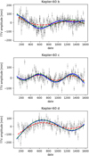 |
Fig. 5 TTVs of the Laplace-resonant chain Kepler-60. See Fig. 4 for the description. |
| In the text | |
 |
Fig. 6 Peak-to-peak TTV amplitudes of the sinusoidal approximation of all of the planets that were analysed in this study. Black points are fits to the pre-extracted timings published by Rowe et al. (2015), which for Kepler-128 and Kepler-60 correspond to the red-dashed curves in Figs. 4 and 5. The coloured diamonds show the peak-to-peak amplitude of the sinusoidal approximation of the best fit of the photo-dynamical model (the green dashed curves in Figs. 4 and 5). The colour indicates the S/Ni of the planet. The agreement between pre-extracted timings and photo-dynamical fit is reduced for lower S/Ni. This is further highlighted in Fig. 7. |
| In the text | |
 |
Fig. 7 Difference between the amplitude of the sinusoidal approximation of both the best solution of the photo-dynamical analysis and pre-extracted transit timings (top). The blue dots correspond to the timings from Rowe et al. (2015), and in orange from Holczer et al. (2016). Reduced chi-squared between the published transit timings and the best solution of the photo-dynamical fit (bottom). |
| In the text | |
 |
Fig. 8 In black and grey, the default and high-mass posteriors of the fit of pre-extracted TTVs from Rowe et al. (2015) by Hadden & Lithwick (2017). In green and blue, we give the posteriors from the RIVERS analysis. Dark green shows the default posterior, light green the high-mass posterior, and blue the final posterior. The full photo-dynamical analysis reduces the prior dependency, thereby increasing massestimate robustness, for most planets of the sample. |
| In the text | |
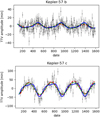 |
Fig. 9 TTVs of the near-resonant system Kepler-57. See Fig. 4 for details. |
| In the text | |
 |
Fig. 10 TTVs of Kepler-24 e at the top. Details are the same as in Fig. 4. Bottom panel shows the mass posteriors of the planets of Kepler-24, depending on the addition of Kepler-24 e to the model; see Fig. 8 for a description. Adding Kepler-24 e helps to better constrain the masses of Kepler-24 b and Kepler-24 c, despite having a highly degenerate mass itself. |
| In the text | |
 |
Fig. 11 Mass-radius relationship of the re-analysed set of Kepler planets with the final posterior. The colour shows the degeneracy metric defined above Eq. (7): black-purple corresponds to well-constrained masses (low prior dependency), while red-yellow shows poorly constrained masses (high prior dependency). The grey background is the mass-radius relationship from RV-estimated masses. |
| In the text | |
 |
Fig. 12 Mass-radius relationship of the robust set of Kepler planets. The colour code shows the equilibrium temperature of the planet, taken from the exoplanet archive (computed assuming a bond albedo of 0.3). |
| In the text | |
 |
Fig. 13 Radius (left) and mass (right) as function of equilibrium temperature of both the re-analysed set of Kepler planets (larger circles with green outline) and the RV-characterised planets. Colour code shows the modelled gas mass fraction of the planets in a logarithmic scale. |
| In the text | |
 |
Fig. A.1 Corner plots of the eccentricities and longitudes of periastron of the default posterior of Kepler-345 b and c. The top-left corner shows the real and imaginary part of 𝒵 and 𝒵2, top-right corner shows the ki = ei cos ϖi and hi = ei sin ϖi variables, bottom left corner shows the ei and ϖi variables, and the bottom right corner shows the |
| In the text | |
Current usage metrics show cumulative count of Article Views (full-text article views including HTML views, PDF and ePub downloads, according to the available data) and Abstracts Views on Vision4Press platform.
Data correspond to usage on the plateform after 2015. The current usage metrics is available 48-96 hours after online publication and is updated daily on week days.
Initial download of the metrics may take a while.


