| Issue |
A&A
Volume 688, August 2024
|
|
|---|---|---|
| Article Number | A211 | |
| Number of page(s) | 21 | |
| Section | Planets and planetary systems | |
| DOI | https://doi.org/10.1051/0004-6361/202450212 | |
| Published online | 26 August 2024 | |
Photo-dynamical characterisation of the TOI-178 resonant chain
Exploring the robustness of transit-timing variations and radial velocity mass characterisations★,★★
1
Observatoire astronomique de l’Université de Genève,
Chemin Pegasi 51,
1290
Versoix,
Switzerland
e-mail: This email address is being protected from spambots. You need JavaScript enabled to view it.
2
Space Research and Planetary Sciences, Physics Institute, University of Bern,
Gesellschaftsstrasse 6,
3012
Bern,
Switzerland
3
Astrobiology Research Unit, Université de Liège,
Allée du 6 Août 19C,
4000
Liège,
Belgium
4
Space sciences, Technologies and Astrophysics Research (STAR) Institute, Université de Liège,
Allée du 6 Août 19C,
4000
Liège,
Belgium
5
Institute of Astronomy, KU Leuven,
Celestijnenlaan 200D,
3001
Leuven,
Belgium
6
Mullard Space Science Laboratory, University College London,
Holmbury St Mary, Dorking,
Surrey
RH5 6NT,
UK
7
Department of Astronomy, Stockholm University,
AlbaNova University Center,
10691
Stockholm,
Sweden
8
Center for Space and Habitability, University of Bern,
Gesellschaftsstrasse 6,
3012
Bern,
Switzerland
9
Department of Physics and Kavli Institute for Astrophysics and Space Research, Massachusetts Institute of Technology,
Cambridge,
MA
02139,
USA
10
Department of Physics, University of Warwick,
Gibbet Hill Road,
Coventry
CV4 7AL,
UK
11
Centre Vie dans l’Univers, Faculté des sciences, Université de Genève,
Quai Ernest-Ansermet 30,
1211
Genève 4,
Switzerland
12
Observatoire Astronomique de l’Université de Genève,
Chemin Pegasi 51,
CH-1290
Versoix,
Switzerland
13
European Space Agency (ESA), European Space Research and Technology Centre (ESTEC),
Keplerlaan 1,
2201 AZ
Noordwijk,
The Netherlands
14
Cavendish Laboratory,
JJ Thomson Avenue,
Cambridge
CB3 0HE,
UK
15
Instituto de Astrofísica de Canarias,
Vía Láctea s/n,
38200
La Laguna,
Tenerife,
Spain
16
Departamento de Astrofísica, Universidad de La Laguna,
Astrofísico Francisco Sanchez s/n,
38206
La Laguna,
Tenerife,
Spain
17
Departamento de Astronomía, Universidad de Chile,
Casilla 36-D,
Santiago,
Chile
18
Instituto de Astronomía, Universidad Católica del Norte,
Angamos 0610,
Antofagasta
1270709,
Chile
19
Admatis,
5. Kandó Kálmán Street,
3534
Miskolc,
Hungary
20
Depto. de Astrofísica, Centro de Astrobiología (CSIC-INTA),
ESAC campus,
28692
Villanueva de la Cañada (Madrid),
Spain
21
Instituto de Astrofisica e Ciencias do Espaco, Universidade do Porto, CAUP,
Rua das Estrelas,
4150-762
Porto,
Portugal
22
Departamento de Fisica e Astronomia, Faculdade de Ciencias, Universidade do Porto,
Rua do Campo Alegre,
4169-007
Porto,
Portugal
23
Space Research Institute, Austrian Academy of Sciences,
Schmiedlstrasse 6,
8042
Graz,
Austria
24
INAF, Osservatorio Astronomico di Padova,
Vicolo dell’Osservatorio 5,
35122
Padova,
Italy
25
Centre for Exoplanet Research, School of Physics and Astronomy, University of Leicester,
Leicester
LE1 7RH,
UK
26
Centre for Exoplanet Science, SUPA School of Physics and Astronomy, University of St Andrews,
North Haugh,
St Andrews
KY16 9SS,
UK
27
CFisUC, Departamento de Física, Universidade de Coimbra,
3004-516
Coimbra,
Portugal
28
Institute of Planetary Research, German Aerospace Center (DLR),
Rutherfordstrasse 2,
12489
Berlin,
Germany
29
INAF, Osservatorio Astrofisico di Torino,
Via Osservatorio, 20,
10025
Pino Torinese To,
Italy
30
Centre for Mathematical Sciences, Lund University,
Box 118,
221 00
Lund,
Sweden
31
Aix-Marseille Université, CNRS, CNES, LAM,
38 rue Frédéric Joliot-Curie,
13388
Marseille,
France
32
ELTE Gothard Astrophysical Observatory,
9700
Szombathely,
Szent Imre h. u. 112,
Hungary
33
SRON Netherlands Institute for Space Research,
Niels Bohrweg 4,
2333 CA
Leiden,
The Netherlands
34
Leiden Observatory, University of Leiden,
PO Box 9513,
2300 RA
Leiden,
The Netherlands
35
Department of Space, Earth and Environment, Chalmers University of Technology,
Onsala Space Observatory,
439 92
Onsala,
Sweden
36
Dipartimento di Fisica, Università degli Studi di Torino,
via Pietro Giuria 1,
10125,
Torino,
Italy
37
National and Kapodistrian University of Athens, Department of Physics,
University Campus, Zografos
157 84,
Athens,
Greece
38
Astronomy Unit, Queen Mary University of London,
Mile End Road,
London
E1 4NS,
UK
39
Department of Astrophysics, University of Vienna,
Türkenschanzstrasse 17,
1180
Vienna,
Austria
40
Institute for Theoretical Physics and Computational Physics, Graz University of Technology,
Petersgasse 16,
8010
Graz,
Austria
41
Instituto de Estudios Astrofísicos, Facultad de Ingeniería y Ciencias, Universidad Diego Portales,
Av. Ejército Libertador 441,
Santiago,
Chile
42
NASA Ames Research Center,
Moffett Field,
CA
94035,
USA
43
Konkoly Observatory, Research Centre for Astronomy and Earth Sciences,
1121
Budapest,
Konkoly Thege Miklós út 15-17,
Hungary
44
ELTE Eötvös Loránd University, Institute of Physics,
Pázmány Péter sétány 1/A,
1117
Budapest,
Hungary
45
Lund Observatory, Division of Astrophysics, Department of Physics, Lund University,
Box 118,
22100
Lund,
Sweden
46
IMCCE, UMR8028 CNRS, Observatoire de Paris, PSL Univ., Sorbonne Univ.,
77 av. Denfert-Rochereau,
75014
Paris,
France
47
Center for Astrophysics, Harvard and Smithsonian,
60 Garden Street,
Cambridge,
MA
02138,
USA
48
Institut d’Astrophysique de Paris, UMR7095 CNRS, Université Pierre & Marie Curie,
98bis blvd. Arago,
75014
Paris,
France
49
Astrophysics Group, Lennard Jones Building, Keele University,
Staffordshire
ST5 5BG,
UK
50
Department of Physics and Astronomy, McMaster University,
1280 Main Street West,
Hamilton,
Ontario
L8S 4L8,
UK
51
INAF, Osservatorio Astrofisico di Catania,
Via S. Sofia 78,
95123
Catania,
Italy
52
Institute of Optical Sensor Systems, German Aerospace Center (DLR),
Rutherfordstrasse 2,
12489
Berlin,
Germany
53
Dipartimento di Fisica e Astronomia “Galileo Galilei”, Università degli Studi di Padova,
Vicolo dell’Osservatorio 3,
35122
Padova,
Italy
54
ETH Zurich, Department of Physics,
Wolfgang-Pauli-Strasse 2,
8093
Zurich,
Switzerland
55
Institut fuer Geologische Wissenschaften, Freie Universitaet Berlin,
Maltheserstrasse 74-100,
12249
Berlin,
Germany
56
Institut de Ciencies de l’Espai (ICE, CSIC),
Campus UAB, Can Magrans s/n,
08193
Bellaterra,
Spain
57
Institut d’Estudis Espacials de Catalunya (IEEC),
08860
Castelldefels (Barcelona),
Spain
58
Department of Earth, Atmospheric and Planetary Sciences, Massachusetts Institute of Technology,
Cambridge,
MA
02139,
USA
59
Department of Aeronautics and Astronautics,
MIT, 77 Massachusetts Avenue,
Cambridge,
MA
02139,
USA
60
HUN-REN-ELTE Exoplanet Research Group,
Szent Imre h. u. 112.,
Szombathely
9700,
Hungary
61
Institute of Astronomy, University of Cambridge,
Madingley Road,
Cambridge
CB3 0HA,
UK
62
Department of Astrophysical Sciences, Princeton University,
Princeton,
NJ
08544,
USA
63
Centro de Astrofísica y Tecnologías Afines (CATA),
Casilla 36-D,
Santiago,
Chile
Received:
2
April
2024
Accepted:
23
May
2024
Abstract
Context. The TOI-178 system consists of a nearby, late-K-dwarf with six transiting planets in the super-Earth to mini-Neptune regime, with radii ranging from to 2.9 R⊕ and orbital periods between 1.9 and 20.7 days. All the planets, but the innermost one, form a chain of Laplace resonances. The fine-tuning and fragility of such orbital configurations ensure that no significant scattering or collision event has taken place since the formation and migration of the planets in the protoplanetary disc, thereby providing important anchors for planet formation models.
Aims. We aim to improve the characterisation of the architecture of this key system and, in particular, the masses and radii of its planets. In addition, since this system is one of the few resonant chains that can be characterised by both photometry and radial velocities, we propose to use it as a test bench for the robustness of the planetary mass determination with each technique.
Methods. We performed a global analysis of all the available photometry from CHEOPS, TESS and NGTS, and radial velocity from ESPRESSO, using a photo-dynamical modelling of the light curve. We also tried different sets of priors on the masses and eccentricity, as well as different stellar activity models, to study their effects on the masses estimated by transit-timing variations (TTVs) and radial velocities (RVs).
Results. We demonstrate how stellar activity prevents a robust mass estimation for the three outer planets using radial velocity data alone. We also show that our joint photo-dynamical and radial velocity analysis has resulted in a robust mass determination for planets c to 𝑔, with precision of ~ 12% for the mass of planet c, and better than 10% for planets d to 𝑔. The new precisions on the radii range from 2 to 3%. The understanding of this synergy between photometric and radial velocity measurements will be valuable for the PLATO mission. We also show that TOI-178 is indeed currently locked in the resonant configuration, librating around an equilibrium of the chain.
Key words: methods: data analysis / techniques: photometric / techniques: radial velocities / planets and satellites: detection / planets and satellites: gaseous planets
The reduced CHEOPS lightcurves are available at the CDS via anonymous ftp to cdsarc.cds.unistra.fr (130.79.128.5) or via https://cdsarc.cds.unistra.fr/viz-bin/cat/J/A+A/688/A211
This study uses CHEOPS data observed as part of the Guaranteed Time Observervation (GTO) programmes CH_PR100031, CH_PR120053 and CH_PR140080.
© The Authors 2024
 Open Access article, published by EDP Sciences, under the terms of the Creative Commons Attribution License (https://creativecommons.org/licenses/by/4.0), which permits unrestricted use, distribution, and reproduction in any medium, provided the original work is properly cited.
This article is published in open access under the Subscribe to Open model. This email address is being protected from spambots. You need JavaScript enabled to view it. to support open access publication.
1 Introduction
The observed architecture of planetary systems, defined as the orbit and composition of their planets, is the outcome of their formation in their proto-planetary disc and long-term evolution (typically on scales of Gyr) after its dispersal. In this context, planetary systems observed in chains of Laplace resonances, where each consecutive pair of planets are in (or close to) a two- body mean-motion resonance (MMR), are of particular interest. Indeed, the fine-tuning and fragility of such orbital configurations ensure that no significant scattering or collision event has taken place since the end of the migration of the planets in the protoplanetary disc (e.g. Mills et al. 2016; Izidoro et al. 2017). Hence, these systems are especially valuable for constraining the outcome of protoplanetary discs and provide important floats for planet formation models.
To date, chains of Laplace resonances have only been observed for a few systems: GJ 876 (Rivera et al. 2010), Kepler-60 (Goździewski et al. 2016), Kepler-80 (MacDonald et al. 2016), Kepler-223 (Mills et al. 2016), TRAPPIST-1 (Gillon et al. 2017; Luger et al. 2017), K2-138 (Lopez et al. 2019), TOI-178 (Leleu et al. 2021a, hereafter L21), TOI-1136 (Dai et al. 2023), and HD 110067 (Luque et al. 2023). All these systems, except GJ 876, are transiting, which provides an opportunity to observe the effect of planet-planet gravitational interactions and, thus, to constrain the masses and eccentricities of the planets via their transit-timing variations (TTVs). For stars that are bright enough, it is also possible to obtain radial velocity (RV) measurements, which can provide complementary constraints on the planetary masses and orbital parameters. Out of the transiting systems cited above, only K2-138, TOI-178, TOI-1136, and HD 110067 have had their RV measurements published so far, while the stars are too faint in the visible (V -mag ≳ 14). Having the possibility to measure planetary masses independently from RVs and TTVs is especially valuable to our understanding of how the choices of noise models and degeneracies between parameters affect the robustness of mass measurements for each technique.
Using data from Transiting Exoplanet Survey Satellite (TESS, Ricker et al. 2015), CHaracterising ExOPlanets Satellite (CHEOPS, Benz et al. 2021; Fortier et al. 2024), and Next Generation Transit Survey (NGTS, Wheatley et al. 2018), L21 reported that the nearby (~63 pc) late-K-type star TOI-178 is a compact system of at least six transiting planets in the superEarth to mini-Neptune regime, with radii ranging from ~1.1 to 2.9 R⊕ and orbital periods of 1.91, 3.24, 6.56, 9.96, 15.23, and 20.71 days. The planetary radii were later refined by Delrez et al. (2023), hereafter D23. The five outer planets form a 2:4:6:9:12 chain of Laplace resonances, while the innermost planets b and c are just wide of the 3:5 MMR, which could indicate that it was previously part of the chain but was then pulled away, possibly by tidal forces (L21).
Using RV measurements obtained with the Echelle SPectrograph for Rocky Exoplanets and Stable Spectroscopic Observations (ESPRESSO, Pepe et al. 2021) installed at ESO’s Very Large Telescope (VLT), L21 were also able to derive preliminary estimates for the masses of the planets, and, thus, their bulk densities (when combined with the radii inferred from the transit photometry). The planetary densities that they found show important variations from planet to planet, jumping for example from ∼1 to 0.2 ρ⊕ between planets c and d. By performing a Bayesian internal structure analysis, they showed that the two innermost planets are likely to be mostly rocky, which could indicate that they have lost their primordial gas envelope through atmospheric escape, while all the other planets appear to contain significant amounts of water and/or gas (see also the independent internal structure analysis by Acuña et al. 2022). However, the planetary densities on which these results were based were constrained by a relatively low number of RV points (46 ESPRESSO points).
In this paper, we re-analyse the data presented in L21 and D23, together with additional CHEOPS observations taken in 2021, 2022, and 2023, TESS sector 69 (2023), and NGTS observations taken in 2021, as described in Sect. 2. The whole analysis was performed by a photo-dynamical fit of all available photometry joint with the fit of available RV measurements, as detailed in Sect. 3. We present the result of our analysis in Sect. 4. In particular, we discuss the robustness of the extracted masses, exploring the effect of the mass-eccentricity degeneracy in TTVs and the effect of activity modelling in RV. Finally, we present our conclusions in Sect. 5.
2 Data
In this study, we used the TESS, CHEOPS, ESPRESSO, and NGTS data presented in L21 and D23. In addition, we used 27 new CHEOPS visits, 8 new NGTS observations, and 4 EulerCam observations that were taken in order to monitor the TTVs of the five outer planets of TOI-178. The new data are available at the CDS. We also added the new data from TESS sector 69.
2.1 CHEOPS
Following D23, the raw data of each visit were reduced with PIPE1 (Brandeker et al. 2022), a point spread function (PSF) photometry package developed specifically for CHEOPS. PIPE first uses a principal component analysis (PCA) approach to derive a PSF template library from the data series. The first five principal components (PCs) together with a constant background are then used to fit the individual PSFs of each image using a least-squares minimisation and measure the target’s flux. The number of PCs to use is a trade-off between following systematic PSF changes and overfitting the noise. For faint stars such as TOI-178, the mean PSF (first PC) is sufficient for a good extraction, and attempts to model the PSF better with more PCs usually introduce noise in the extracted light curve. Some advantages of using PSF photometry rather than aperture photometry for faint targets are as follows: (1) the contributions to the signal of each pixel over the PSF are weighted according to noise so that higher S/N photometry can be extracted; (2) cosmic rays and bad pixels (both hot and telegraphic) are easier to filter out or give lower weight in the fitting process; (3) PSF photometry is less sensitive to contamination from nearby background stars; (4) the background is fit simultaneously with the PSF for the same pixels, which can be an advantage if there is some spatial structure. For each visit, we then filter out all the data for which the background contamination rises above 300 [electrons/pixel/exposure]. The raw data can be found on DACE2. The detrended data are shown in Fig. 1, and the details of the CHEOPS visit can be found in Tables A.1 and A.2.
2.2 TESS
TESS observed TOI-178 for the first time during Cycle 1+Sec- tor 2 of its primary mission (22 August to 20 September 2018). These data, obtained with a 2-min cadence, were previously presented in L21 and we include them in our global analysis. TESS observed again TOI-178 during Cycle 3+Sec- tor 29 and Cycle 5+Sector 69 of its extended mission, from 26 August to 22 September 2020 (presented in D23) and from 25 August to 20 September 2023. The data were processed with the TESS Science Processing Operations Center (SPOC) pipeline (Jenkins et al. 2016) at NASA Ames Research Center. We retrieved the 2-min cadence Pre-search Data Conditioning Simple Aperture Photometry (PDCSAP, Stumpe et al. 2012, 2014; Smith et al. 2012) from the Mikulski Archive for Space Telescopes3 (MAST), using the default quality bitmask. The detrended data are shown in Fig. 2.
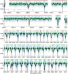 |
Fig. 1 Detrended light curves from CHEOPS as described in Sects. 2.1 and 3.3 The unbinned data are shown as blue points and the data from the 30 min bins are shown as green circles. The best fitting transit model for the system is shown in black; the associated parameter values are from the final posterior shown in Tables 2 and 3. Vertical lines indicate the planet that is transiting, unflagged transits are caused by planet b. Each line contains about six days of observation. Data published in L21 are indicated by a red upper line, the one published in D23 by an orange upper line, and new data by a green upper line. The raw and detrended data are available at the CDS. |
2.3 NGTS
We also included in our global analysis the light curves obtained with the NGTS that were previously published in L21, as well as eight additional transit observations that were obtained between the dates of 23 June 2021 and 3 November 2021. The NGTS photometric facility consists of 12 independently operated robotic telescopes each with a 20 cm diameter aperture and a field-of-view of 8 square-degrees. Using multiple NGTS telescopes to simultaneously observe the same star has been shown to yield vast improvements in the photometric precision compared to observing with a single telescope (Smith et al. 2020; Bryant et al. 2020) and TOI-178 was observed using this high-precision multi-telescope observing mode. We observed three transits of TOI-178d, two transits of TOI-178e, two transits of TOI-178f, and one transit of TOI-178g. The NGTS observations were all performed using the custom NGTS filter (520–890 nm) at a cadence of 13 s and were reduced using a custom aperture photometry pipeline, which utilises the SEP package (Bertin & Arnouts 1996; Barbary 2016) to perform the source extraction and also automatically selects comparison stars which are similar to TOI-178 in magnitude, colour, and CCD position using Gaia DR2 (Gaia Collaboration 2018). For more details on the reduction, we refer to Bryant et al. (2020). The NGTS light curves used are displayed in Fig. 3. We refer to L21 and references therein for more information about the previously published NGTS data and their reduction.
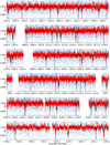 |
Fig. 2 Detrended light curves from TESS as described in Sects. 2.2 and 3.3. The unbinned data are shown as blue points and the data from the 30 min bins are shown as red circles. The best fitting transit model for the system is shown in black; the associated parameter values are from the final posterior shown in Tables 2 and 3. Each line contains about 11 days of observation. The detrended data are available at the CDS. |
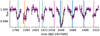 |
Fig. 3 Detrended light curves from NGTS as described in Sects. 2.3 and 3.3. Data in 30 min bins are shown as purple circles. The best-fitting transit model for the system is shown in black; the associated parameter values are from the final posterior shown in Tables 2 and 3. The line contains about two days of observation, each visit containing the data taken by respectively 7, 4, 3, 4, 4, 4, 3, 4, and 5 of the NGTS telescopes. The unbinned data are not shown because the scatter is much larger than the than the flux range shown here. The raw and detrended data are available at the CDS. |
2.4 EulerCam
Multiple transits of planets d, e, and f were observed with the EulerCam instrument between 2021-08-11 and 2021-10-20. EulerCam is a CCD imager installed at the Cassegrain focus of the 1.2m Leonhard Euler telescope at La Silla observatory (Lendl et al. 2012). We used the broadband NGTS filter for our observations to maximise the signal-to-noise ratio (S/N). The data were reduced using the standard EulerCam pipeline, which performs basic image calibration and relative aperture photometry. The optimal aperture and reference stars are selected by minimising the residual RMS of the final light curve. The EulerCam observations took place simultaneously to CHEOPS and (as expected for ground-based data) show much lower precision (RMS in the 900–1800 ppm range). We eventually excluded them from our final analysis, but we show them in Fig. B.1 for completeness.
2.5 ESPRESSO
The RV data, presented in L21, consist of 46 ESPRESSO points. Each measurement was taken in high resolution (HR) mode with an integration time of 20 min using a single telescope (UT) and slow read-out (HR 21). The source on fibre B is the Fabry– Perot interferometer. Observations were made with a maximum airmass of 1.8 and a minimum 30° separation from the Moon.
3 Data analysis
3.1 Stellar properties
In this study, we use the stellar properties that were updated by D23. These properties are summarized in Table 1.
3.2 Approach
The transit timing variations expected for TOI-178 were explained in Sect. 6.4 and illustrated in Fig. 14 of L21. A dominant feature of these TTVs is the effect of the proximity of two-body MMRs (Lithwick et al. 2012), which induce sinusoidal TTVs with a period of ≈260 days (called super-period) on the five planets that are part of the resonant chain (planets c to g). Transit timing variations due to the proximity of two-body MMRs are known to present a mass-eccentricity degeneracy at first order in the eccentricities (Boué et al. 2012; Lithwick et al. 2012). This degeneracy may be broken if either higher harmonics of the super-period (Hadden & Lithwick 2016), the short-term chopping effect (Deck & Agol 2015), or the long-term evolution in the resonance can be constrained.
To check the robustness of the masses we derive, we followed Hadden & Lithwick (2017) and try out priors that pull the solution toward opposite directions of the degeneracy. We used their ‘default’ prior, which is log-uniform in planet masses and uniform in eccentricities, and their ‘high-mass’ prior, which is uniform in planet masses and log-uniform in eccentricities. In addition, following Leleu et al. (2023), we performed a third fit, using log-uniform mass prior and the Kipping (2013) prior for the eccentricity: a β-distribution of parameters α = 0.697 and β = 3.27. The posterior associated with this set of priors is referred to as the ‘final’ posterior. Then, following Leleu et al. (2023), we quantify the robustness of the mass determination by studying the difference between the mass posteriors using the quantity, ΔM:
 (1)
(1)
which estimates the departure of the median of the ‘default’ and ‘high-mass’ posteriors from the median of the ‘final’ posterior, in units of the error bars of the ‘final’ posterior. More precisely:
 (2)
(2)
where mhigh,0 is the maximum between the medians of the ‘default’ and ‘high-mass’ posterior, mfinal,0 is the median of the ‘final’ posterior, and mtinal,+σ is the 0.84 quantile of the ‘final’ posterior. ∆M+ = 0 if mhigh,0.
 (3)
(3)
where mlow,0 is the minimum of the default and high-mass posterior medians, and mfinal −σ is the 0.16 quantile of the final posterior. ∆M2212= 0if mlow,0 >mfinal,0. The values of ∆M obtained for each planet is given in Tables 2 and 3, and discussed in Sect. 4.3.
Transit timing variations can be studied by pre-extracting all the transit timings of the planets, then fitting these transit timings. Alternatively, we can analyse TTVs using a photo-dynamical model (Ragozzine & Holman 2010); in which the ideal light-curve, accounting for TTVs, is modelled and then fit to the data. Leleu et al. (2023) showed that photo-dynamical analysis often allows for a more robust mass estimate, especially for systems harbouring planets whose individual transit S/N is low (typically ≲ 3.5). We therefore performed a photo-dynamical analysis of the data.
Properties of the host star TOI-178.
Fitted and derived properties of the planets of TOI-178.
Fitted and derived properties of the planets of TOI-178.
3.3 Data modelling
We performed a joint analysis of all available transit events as well as the RV data. The gravitational interaction of the five resonant planets (c to g) was also taken into account. For these planets, we used wide, flat priors for the mean longitude, period, impact parameter, and ratio of the radius of the planet over the radius of the star, Rp/R★. The mass, e cos ϖ, and e sin ϖ priors were given in Sect. 3.2. The stellar density and radius have Gaussian priors, with values given in Table 1.
3.3.1 Photometry
The photo-dynamical model of the planetary signals, presented in detail in Leleu et al. (2021b, 2023), is computed by predicting transit timings using the TTVfast package (Deck et al. 2014) for the outer five planets and a circular orbit for TOI-178b, as well as modeling the transits of each planet using the batman package Kreidberg (2015). We modelled the instrumental sys-tematics as well as stellar activity using a linear combination of indicators and B-splines. We used B-splines as functions of time for all photometric data and an additional B-spline is added with respect to the roll-angle for each CHEOPS visit. The temporal B-splines have nodes separated by 0.4 days for all photometry and the periodic B-splines on the roll angle for CHEOPS have nodes separated by 0.1 radian. For CHEOPS, we used as indicators the telescope tube temperature, the position of the centroid along the Y direction, and the background contamination. For NGTS, we used the airmass. For TESS, the light curves were pre-detrended so no indicator were used. This model (indicators and B-splines) only introduces linear parameters. To accelerate the exploration of the parameter space, we compute the likelihood marginalized over these linear parameters, using the linmarg4 python package (Leleu et al. 2023). The limb-darkening parameters have Gaussian priors computed by LDCU (Deline et al. 2022) for each photometric instrument. In addition, a jitter term was added per instrument with a flat prior.
3.3.2 Radial velocities
The RV model of the planetary signals is also computed using the TTVfast package (Deck & Agol 2016) for the five outer planets and a circular model for TOI-178b. We fitted these data by modeling the planets’ orbits as well as stellar activity using a Gaussian process (GP) model trained simultaneously on the RVs and ancillary activity indicators using the spleaf5 package with the FENRlR two modes - four harmonics – Matérn 1/2 kernel; see Appendix D and Hara & Delisle (2023). The GP is trained simultaneously on the RVs, the FWHM, and the Hα activity indicators.
4 Results of the data analysis
In total, the photodynamical+RV fit has 96 free parameters. For the ‘final’ posterior, the MCMC ran for 4.2 × 10⁶ steps. To estimate the convergence of the fit, we computed the integrated auto correlation time of all parameters. Our convergence criterion is that the length of the chain is at least 300 times the longest integrated auto correlation time. For the ‘final’ posterior, we used a burn-in of 7 × 10⁵ samples. The remaining chain is 426 times longer than the longest integrated auto correlation time.
The transit timings estimated for each planet, as well as 300 samples of the final posterior, can be found at the CDS. In particular, the transit timings are propagated until 2030, to be usable for follow-up observations of the system.
4.1 Recovered TTV signal
Figures 4 and 5 show the TTVs of the full fit model for both the ‘default’ and ‘highmass’ sets of priors, along with estimations of individual transit timings for each instrument. In these TTV plots, in addition to the super-period at ~260 days visible for all planets, the long-term evolution of the resonant angles start to be visible for planets c, d, and e. The saw-tooth shape of the chopping effect (Deck & Agol 2015) can be seen on the posterior of planets f and 𝑔.
We also fit the individual transit timings to illustrate how each portion of the TTVs curve is constrained. These individual transit timings were estimated by additional fits of the light curves, fixing all parameters but the transit timings at their values in the best sample of the ‘final’ posterior. Then, for each half of the TESS sectors, CHEOPS visit, and NGTS observation, we fit the transit timings of the planet along with the noise model. The timings are initialised at their position in the best fit of the ‘final’ posterior, with a Gaussian prior centred on that value and a standard deviation of 30 min. These individual transit timings are shown as colored circles in Figs. 4 and 5. While individual transit timings follow the TTV pattern recovered by the photo-dynamical fit for planets d to g. For planet c, the median error of the transit timings is larger than the amplitude of the TTV signal. The median standard deviation of the timing derived from the photo-dynamical model (0.86 min) highlights the necessity of using photo-dynamical modelling for planets with low-S/N transits (Leleu et al. 2023).
A downside of the photo-dynamical analysis is its model dependency: we have to choose a priori how many planets we are considering in the modelling of the light curves, as well as the effect of potential missed planets can be hard to identify on the light curve residuals. Having the individual transit timings also allows us to check if there are hints of additional planets in the resonant chain, for example, at orbital periods larger than Pg = 20.7 days. Indeed, the effect of this additional planet, which is not modelled by the five-resonant planet model, could become apparent when subtracting the timing from the photo-dynamical analysis to the individual transit timings. However, we did not find strong evidence of a planet significantly impacting the TTVs of the observed planets.
4.2 Recovered planetary parameters
The planetary masses, radii, transit parameters and Jacobi orbital elements at epoch 1352.55018 [BJD-2457000] are given in Tables 2 and 3 for the ‘final’ posterior of the photo-dynamical fit and the combined photo-dynamical and radial-velocity fits, while Tables C.1 and C.2 shows the fitted stellar and noise parameters.
In this joint analysis, the final posterior reaches a precision of 12% for the mass of planet c, while the precision on the mass of planets d to 𝑔 is better than 10%. The precision we reach for planet b remains similar to the one published in L21, since the planet does not induce any significant TTVs on the other planets of the system. The precision on the planetary radius ranges from ≈3% for planet b to better than 2% for the largest planet of the system. Figure 6 shows the mass-radius relation of the TOI-178 planets derived in this study with respect to the planets whose mass was characterised by either TTVs (green) or RV (blue). These reference planets were chosen for their robustness to the choice of prior for the TTV population and for their precision for the RV population. The RV-characterised planets appear to be denser than the TTV-characterised ones, although we note that selecting RV-characterised planets based on their precision might bias that population toward denser mass-radius combinations. The apparent discrepancy between the TTV and RV-characterised planets has been heavily discussed (e.g. Wu & Lithwick 2013; Weiss & Marcy 2014; Mills & Mazeh 2017; Hadden & Lithwick 2017; Cubillos et al. 2017; Millholland et al. 2020; Leleu et al. 2023; Adibekyan et al. 2024). In particular, Hadden & Lithwick (2017) put forward as a possible explanation a selection bias, since TTVs tend to allow the characterisation of small planets on larger orbital periods and, thus, cooler orbits, than the bulk of the RV characterisation. It has also been proposed that the systems formed in different environments, such as a different amount of available iron during the planets’ formation (Adibekyan et al. 2024). The gaseous planets of TOI-178 appear to be on the lower end of density for their respective radius, more akin to the sub-population that was characterised using TTVs. The possibility to characterise TOI-178 both by RV and TTVs makes this system especially relevant to study this discrepancy. With the preliminary masses obtained by the RV data, L21 showed that the density of the planets appeared to not evolve monotonically with respect to the equilibrium temperature of the planets. With our updated planetary masses and radii, we retrieved a similar trend, as seen in Fig. 7.
Finally, L21 claimed that the system is in a chain of Laplace resonances. Using the preliminary mass determination, averaged periods and assuming zero initial eccentricities, they showed that the system was within the stability domain of the three-body resonance chain. Thanks to the joint photo-dynamical and RV fit, we now have estimations of the instantaneous orbital elements of each planet at a given date, see Tables 2 and 3. Using 300 randomly-selected samples of the final posterior, we can simulate the future evolution of the Laplace angles ψ1 = 1λc − 4λd + 3λe, ψ2 = 2λd − 5λe + 3λf, and ψ3 = 1λe − 3λf + 2λ𝑔, where λ is the mean longitude of the planet. Figure 8 shows the three-sigma envelope of the evolution of these angles over the next 1000 yr. Although we lose the information on the phase of the libration after a few decades, we can see that our full posterior yields librating angles, confirming that the system is indeed currently librating in the chain of Laplace resonances, around the equilibrium described in Table 6 of L21.
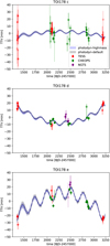 |
Fig. 4 Transit timing variations observed for TOI-178 c, d and e. The filled area correspond to the 1σ posterior of the photo-dynamical fits presented in Sect. 3.2. The error bars show an estimation of the 1σ interval for the mid-transit timing of individual transits for each instrument, with transparency depending on the precision of the timings. See the text for more details. |
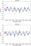 |
Fig. 5 Mass-radius relationship of the TOI-178 planets (final posterior), compared with the super-Earth to Mini-Neptune populations for which the mass was derived through RV (Otegi et al. 2020) and TTVs (Hadden & Lithwick 2017; Leleu et al. 2023). The composition lines ‘terrestrial Earth-like’, in solid brown, and pure MgSiO3 ‘rocky’, in dashed brown, are taken from Zeng et al. (2016). |
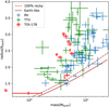 |
Fig. 6 Mass-radius relationship of the TOI-178 planets (final posterior), compared with the super-Earth to Mini-Neptune populations for which the mass was derived through RV (Otegi et al. 2020) and TTVs (Hadden & Lithwick 2017; Leleu et al. 2023). The composition lines ‘terrestrial Earth-like’, in solid brown, and pure MgSiO3 ‘rocky’, in dashed brown, are taken from Zeng et al. (2016). |
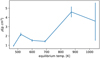 |
Fig. 7 Mean density of the TOI-178 planets as a function of their equilibrium temperature. |
4.3 Robustness of the retrieved masses
To estimate the robustness of mass determination with each technique, we performed RV fits, photo-dynamical fits and joint fits with the sets of priors defined in Sect. 3.2. We note that for the RV fit, the eccentricity of the planets is set to zero and therefore the ‘default’ and ‘final’ sets of priors are identical. For the RV fits, we additionally tested several activity models (see Appendix D), as they could have an impact on the mass determination (e.g. Bonfils et al. 2018; Ahrer et al. 2021).
We show in Fig. 9 a summary of the mass posteriors from these analyses. We can see from Fig. 9 that the RV mass determination (black and gray) is robust for the three inner planets, in the sense that the posteriors for the default and the high-mass priors agree well. The three outer planets’ masses are more sensitive to the priors. We also note that these planets’ masses are also more sensitive to a change of stellar activity model (see Appendix D). We recall that the stellar rotation period was estimated to be about 35 d by L21, and that we only have 46 RV measurements over 113 days. It is thus very challenging to train a GP at the same time as fitting for the six planets’ masses on these data. Since we noticed a strong model sensitivity for the three outer planets’ mass, we selected one of the activity models that exhibited large uncertainties for these three parameters for the subsequent analyses (joint fit), to avoid biasing the final mass estimates for these planets (see Appendix D). This does not mean that the chosen activity model is intrinsically better, and better constraining the activity model and the planets’ masses from RV would require more measurements.
The posteriors of the masses from the photo-dynamical fit for the different sets of priors are shown in blue in Figs. 9. As explained in Sect. 3.2, the ∆M criterion quantifies the prior-dependency of these masses. Also, ∆M = 0 indicates that the posteriors of the default, high-mass, and final fit all perfectly agree, while ∆M = 1 indicates that the median of the default or high-mass posteriors lies exactly at 1 – σ from the median of the final posterior. Leleu et al. (2023) set an arbitrary limit at ∆M = 1.3 to estimate if the retrieved mass was degenerate or not. From the photo-dynamical fit alone, planets c, d, e, and f have robust masses, with values of ∆M = 0.72, 0.84, 0.54, and 0.93, while the mass of planet g shows a greater dependency on priors, with ΔM = 1.34 (see Tables 2 and 3).
Overall, the photo-dynamical model gives better mass precision than the RV fit for planets d to e, while having a much lower prior dependency for the three outer planets. The mass of TOI-178c is fully consistent between the two techniques, which is important to note, since this mass is also the least sensitive to the choice of activity model or mass prior in the RV analysis (see Appendix D). For TOI-178d the median of the ‘default’ photo-dynamic posterior is 3-σ away from the RV ‘default’ posterior. However, while the posteriors shown in Fig. 9 display a low dependency on the mass prior, the dependency to the choice of activity model is bigger, see Appendix D.
When looking at the posteriors of the joint fit, in green in Fig. 9, we can see that most of the constraints on the mass come from the photo-dynamical model, as the joint mass posteriors (green) remain close to the photo-dynamical posteriors (blue). We nonetheless note a general improvement in the robustness of the determined mass, as the prior dependency (ΔM in Tables 2 and 3) is generally smaller in the joint fit than in the photo-dynamical fit alone, beside a slight increase to 1.15 for TOI-178f.
Finally, we estimated the robustness of the derived masses to the existence of a seventh planet in the resonant chain, with more details given in Appendix E. The outcome of this test is reported by the cyan error bars in Fig. 9. Overall, adding an additional planet to the model does not significantly change the derived mass for the six known planets. These results are in agreement with the findings of Leleu et al. (2023), namely, that having the proper TTV model (number of planets in the system) goes hand-in-hand with having a low prior dependency (low value of ΔM) for the retrieved masses of the system.
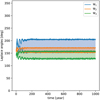 |
Fig. 8 Three-sigma envelope of the evolution of the Laplace angles Ψ1, Ψ2, and Ψ3 over 1000 yr for the final posterior. |
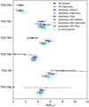 |
Fig. 9 Mass determinations for different datasets and choices of priors. In black: the posterior from the RV analysis with the FENRIR two modes – four harmonics – Matérn 1/2 model (see Appendix D). The blue posteriors are from the photo-dynamical model alone, while the green posteriors are from the joint photo-dynamical and RV fits. The ‘default’, ‘high-mass’, and ‘final’ set of priors are defined in Sect. 3.2. The cyan posterior synthesise the best fits of all our models with additional planets in the resonant chain, see Appendix E. The photodyn ‘final’ and photodyn+RV ‘final’ are the cases reported in Tables 2 and 3. |
5 Summary and conclusion
In this study, we present a joint analysis of all available data for the TOI-178 system. We combined a photo-dynamical analysis of the data taken by TESS, CHEOPS, and NGTS, with the RVs taken by ESPRESSO. In addition, we explore the robustness of the derived masses by comparing the results of the joint fit to the mass constraints obtained by RV and photometry independently.
We show that the available RVs on their own do not enable us to fully distinguish the planetary signal from stellar activity for the three outer planets. In particular, for planet g, when fitting the RV data with different activity models and mass priors, it results in a large range of unphysical mass measurements, an issue that was also reported for example by Lopez et al. (2019) in the case of K2-138f. Arguably, the case of TOI-178d is the most intriguing, with all activity models and choice of priors giving relatively consistent masses using the RV data alone. These masses are at least 2 σ away from the results of the photo-dynamical fit. On the other hand, the techniques fully agree for the mass of TOI-178c, which is reassuring since it is the mass that is the most robust to the choice of activity model and mass prior across all our tests (see Appendix D).
We show that the photo-dynamical analysis is able to retrieve robust masses on its own (low dependency on the chosen set of priors) for planets c to f, and our joint photo-dynamical+RV analysis is able to retrieve robust masses for planets c to g. This highlights the need for thorough follow-up campaigns for the characterisation of multi-planetary systems, as well as the development and calibration of robustness criteria for the derived planetary masses. For these criteria, bright resonant systems such as TOI-178 have an important role to play since its planetary masses can be obtained independently by both RV and TTVs. Obtaining these two independent mass measurements for the same planets can ensure the accuracy of these measurements and therefore help with the calibration of the robustness criteria. In the case of TOI-178, additional transit measurements would further increase our confidence in the robustness of the TTV masses, while additional RV measurements are necessary both to obtain better constraints on planet b (which is outside of the chain). In addition, it would be helpful to distinguish the signal of the three outer planets from the stellar activity. These observations also enable a better understanding of the synergies between photometric and RV measurements on a given system, which will be key to achieve the full potential of the upcoming PLATO mission (Rauer et al. 2014).
Thanks to the intensive follow-up effort, TOI-178 now has one of the best characterised architectures of resonant chains of sub-Neptunes. We were able to show that the system is indeed librating inside the Laplace resonant chain, around the equilibrium that was described in Sect. 6.2 of L21. We also reached a precision of ~12% for the mass of planet c, and better than 10% for planets d, e, f, and g. The new precisions on the radii range from ≈3% for planet b to better than 2% for planet g. We note that we were not able to improve the mass of planet b as it is not interacting with the resonant chain. The newly derived mass and radius of c appear to depart from the 100% rocky composition that was favoured in L21, implying that a gaseous envelope is necessary to reproduce the observed density. Planet d to g remain akin to the TTV-characterised Mini-Neptunes (see Fig. 6), making of TOI-178 a key system in the study of the apparent mass-radius discrepancy between TTV and RV-characterised population (Wu & Lithwick 2013; Weiss & Marcy 2014; Mills & Mazeh 2017; Cubillos et al. 2017; Hadden & Lithwick 2017; Millholland et al. 2020; Leleu et al. 2023; Adibekyan et al. 2024). We also retrieve the non-monotonous density variations as function as the distance to the star that was hinted at by L21.
These new constraints will allow for better comparisons with models of the formation and evolution of planetary systems (e.g. Emsenhuber et al. 2021; Izidoro et al. 2022), as well as enabling the exploitation of the JWST transmission spectrum of the system to their full potential.
Acknowledgements
CHEOPS is an ESA mission in partnership with Switzerland with important contributions to the payload and the ground segment from Austria, Belgium, France, Germany, Hungary, Italy, Portugal, Spain, Sweden, and the United Kingdom. The CHEOPS Consortium would like to gratefully acknowledge the support received by all the agencies, offices, universities, and industries involved. Their flexibility and willingness to explore new approaches were essential to the success of this mission. CHEOPS data analysed in this article will be made available in the CHEOPS mission archive (https://cheops.unige.ch/archive_browser/). This work has been carried out within the framework of the NCCR PlanetS supported by the Swiss National Science Foundation under grants 51NF40_182901 and 51NF40_205606. A.L. acknowledges support of the Swiss National Science Foundation under grant number TMSGI2_211697. The Belgian participation to CHEOPS has been supported by the Belgian Federal Science Policy Office (BELSPO) in the framework of the PRODEX Program, and by the University of Liège through an ARC grant for Concerted Research Actions financed by the Wallonia-Brussels Federation. L.D. thanks the Belgian Federal Science Policy Office (BELSPO) for the provision of financial support in the framework of the PRODEX Programme of the European Space Agency (ESA) under contract number 4000142531. The contributions at the Mullard Space Science Laboratory by E.M.B. have been supported by STFC through the consolidated grant ST/W001136/1. A.Br. was supported by the SNSA. This work has been carried out within the framework of the NCCR PlanetS supported by the Swiss National Science Foundation under grants 51NF40_182901 and 51NF40_205606. T.Wi. acknowledges support from the UKSA and the University of Warwick. M.L. acknowledges support of the Swiss National Science Foundation under grant number PCEFP2_194576. This project has received funding from the Swiss National Science Foundation for project 200021_200726. It has also been carried out within the framework of the National Centre of Competence in Research PlanetS supported by the Swiss National Science Foundation under grant 51NF40_205606. The authors acknowledge the financial support of the SNSF. M.L. and H.C. acknowledge support of the Swiss National Science Foundation under grant number PCEFP2_194576. M.N.G. is the ESA CHEOPS Project Scientist and Mission Representative, and as such also responsible for the Guest Observers (GO) Programme. MNG does not relay proprietary information between the GO and Guaranteed Time Observation (GTO) Programmes, and does not decide on the definition and target selection of the GTO Programme. Y.Al. acknowledges support from the Swiss National Science Foundation (SNSF) under grant 200020_192038. We acknowledge financial support from the Agencia Estatal de Investigación of the Ministerio de Ciencia e Innovación MCIN/AEI/10.13039/501100011033 and the ERDF “A way of making Europe” through projects PID2019-107061GB-C61, PID2019-107061GB-C66, PID2021-125627OB-C31, and PID2021-125627OB-C32, from the Centre of Excellence “Severo Ochoa” award to the Instituto de Astrofísica de Canarias (CEX2019-000920-S), from the Centre of Excellence “María de Maeztu” award to the Institut de Ciències de l’Espai (CEX2020-001058-M), and from the Generalitat de Catalunya/CERCA programme. This research was funded in whole or in part by the UKRI, (Grants ST/X001121/1, EP/X027562/1). We acknowledge financial support from the Agencia Estatal de Investigación of the Ministerio de Ciencia e Innovación MCIN/AEI/10.13039/501100011033 and the ERDF “A way of making Europe” through projects PID2019-107061GB-C61, PID2019-107061GB-C66, PID2021-125627OB-C31, and PID2021-125627OB-C32, from the Centre of Excellence “Severo Ochoa” award to the Instituto de Astrofísica de Canarias (CEX2019-000920-S), from the Centre of Excellence “María de Maeztu” award to the Institut de Ciències de l’Espai (CEX2020-001058-M), and from the Generalitat de Catalunya/CERCA programme. S.C.C.B. acknowledges support from FCT through FCT contracts nr. IF/01312/2014/CP1215/CT0004. The contributions from MPB were carried out within the framework of the National Centre of Competence in Research PlanetS supported by the Swiss National Science Foundation under grants 51NF40_182901 and 51NF40_205606. The authors acknowledge the financial support of the SNSF. L.Bo., G.Br., V.Na., I.Pa., G.Pi., R.Ra., G.Sc., V.Si., and T.Zi. acknowledge support from CHEOPS ASI-INAF agreement n. 2019-29-HH.0. C.B. acknowledges support from the Swiss Space Office through the ESA PRODEX program. A.C.C. acknowledges support from STFC consolidated grant number ST/V000861/1, and UKSA grant number ST/X002217/1. P.E.C. is funded by the Austrian Science Fund (FWF) Erwin Schroedinger Fellowship, program J4595-N. This project was supported by the CNES. This work was supported by FCT - Fundação para a Ciência e a Tecnologia through national funds and by FEDER through COM-PETE2020 through the research grants UIDB/04434/2020, UIDP/04434/2020, 2022.06962.PTDC. O.D.S.D. is supported in the form of work contract (DL 57/2016/CP1364/CT0004) funded by national funds through FCT. B.-O.D. acknowledges support from the Swiss State Secretariat for Education, Research and Innovation (SERI) under contract number MB22.00046. M.F. and C.M.P. gratefully acknowledge the support of the Swedish National Space Agency (DNR 65/19, 174/18). DG gratefully acknowledges financial support from the CRT foundation under Grant No. 2018.2323 “Gaseous or rocky? Unveiling the nature of small worlds”. E.G. gratefully acknowledges support from the UK Science and Technology Facilities Council (STFC. project reference ST/W001047/1). M.G. is an F.R.S.-FNRS Senior Research Associate. F.H. is supported by an STFC studentship. C.He. acknowledges support from the European Union H2020-MSCA-ITN-2019 under Grant Agreement no. 860470 (CHAMELEON). KGI is the ESA CHEOPS Project Scientist and is responsible for the ESA CHEOPS Guest Observers Programme. She does not participate in, or contribute to, the definition of the Guaranteed Time Programme of the CHEOPS mission through which observations described in this paper have been taken, nor to any aspect of target selection for the programme. J.S.J. greatfully acknowledges support by FONDE-CYT grant 1201371 and from the ANID BASAL project FB210003. K.W.F.L. was supported by Deutsche Forschungsgemeinschaft grants RA714/14-1 within the DFG Schwerpunkt SPP 1992, Exploring the Diversity of Extrasolar Planets. This work was granted access to the HPC resources of MesoPSL financed by the Région Île-de-France and the project Equip@Meso (reference ANR-10-EQPX-29-01) of the programme Investissements d’Avenir supervised by the Agence Nationale pour la Recherche. P.M. acknowledges support from STFC research grant number ST/R000638/1. This work was also partially supported by a grant from the Simons Foundation (PI Queloz, grant number 327127). N.C.Sa. acknowledges funding by the European Union (ERC, FIERCE, 101052347). Views and opinions expressed are however those of the author(s) only and do not necessarily reflect those of the European Union or the European Research Council. Neither the European Union nor the granting authority can be held responsible for them. A.S. acknowledges support from the Swiss Space Office through the ESA PRODEX program. S.G.S. acknowledge support from FCT through FCT contract nr. CEECIND/00826/2018 and POPH/FSE (EC). The Portuguese team thanks the Portuguese Space Agency for the provision of financial support in the framework of the PRODEX Programme of the European Space Agency (ESA) under contract number 4000142255. Gy.M.Sz. acknowledges the support of the Hungarian National Research, Development and Innovation Office (NKFIH) grant K-125015, a a PRODEX Experiment Agreement No. 4000137122, the Lendulet LP2018-7/2021 grant of the Hungarian Academy of Science and the support of the city of Szombathely. V.V.G. is an F.R.S.-FNRS Research Associate. J.V. acknowledges support from the Swiss National Science Foundation (SNSF) under grant PZ00P2_208945. N.A.W. acknowledges UKSA grant ST/R004838/1. This work is based in part on data collected under the NGTS project at the ESO La Silla Paranal Observatory. The NGTS facility is operated by a consortium institutes with support from the UK Science and Technology Facilities Council (STFC) under projects ST/M001962/1, ST/S002642/1 and ST/W003163/1 A.C.M.C. acknowledges support from the FCT, Portugal, through the CFisUC projects UIDB/04564/2020 and UIDP/04564/2020, with DOI identifiers 10.54499/UIDB/04564/2020 and 10.54499/UIDP/04564/2020, respectively. C.M. acknowledges support from the Swiss National Science Foundation under grant 200021_204847 “PlanetsInTime”.
Appendix A CHEOPS
The logs of the CHEOPS visit used in this study are given in Tables A.1 and A.2.
log of CHEOPS visits
CHEOPS visits
Appendix B EulerCam
The detrended Eulercam data are shown in Fig. B.1
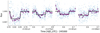 |
Fig. B.1 Detrended light curves from EulerCam as described in Sect. 2.4. The unbinned data are shown as blue points and the data from the 30 min bins are shown as purple circles. The best-fitting transit model for the system is shown in black. |
Appendix C Posteriors of the stellar and noise parameters
The posteriors of the stellar and noise parameters are given in Tables C.1 and C.2.
Fitted properties of the star and noise parameters
Fitted properties of the star and noise parameters
Appendix D Robustness of the RV mass estimation and activity modelling
Poorly modelled noise sources can introduce biases, in particular in parameters which are always positive such as mass and eccentricity (Hara et al. 2019). To test the robustness of the mass estimates of the six planets obtained from the ESPRESSO RVs, we analyzed the RV time series using different activity models and different mass priors. The results are shown in Fig. D.1. In all cases, we fixed the periods and phases of the planets to the values of Delrez et al. (2023, median values from Tables 3 and 4). We assumed circular orbits and only let the semi-amplitudes of the RV signals to vary. We tested each activity model with a log-uniform (default) prior on the semi-amplitudes and with a uniform (high-mass) prior. In the case of the high-mass prior, we also allow for negative semi-amplitudes (hence, negative planetary masses). A negative semi-amplitude means that the signal is found in opposite phase with what is expected from the transit. We allow for this to better assess the reliability of the mass constraints we get from RVs and the dependency of the results with respect to the activity model and the mass prior. We used the spleaf GP package (Delisle et al. 2020), with either the ESP kernel (Delisle et al. 2022) or the FENRIR kernel (Hara & Delisle 2023). In both cases, the GP is trained simultaneously on the RVs, FWHM, and the Hα activity indicators.
The ESP kernel is an approximation of the widely spread SEP (squared-exponential periodic) kernel (e.g. Aigrain et al. 2012). The approximation is truncated at a given number of harmonics of the rotation period. We used between two (rotation period + semi-period) and five harmonics.
The FENRIR kernel is, in its data-driven form that we used here, a more flexible kernel which is also decomposed into harmonics of the rotation period, but with free coefficients. As for the ESP kernel, we used between two and five harmonics.
We also tested different decay envelopes (Matérn 1/2 and 3/2), as well as one or two modes. Having two modes is equivalent to having two independent FENRIR processes with the same hyper-parameters but different amplitudes. It is thus a much more flexible model than the one-mode FENRIR kernel.
From Fig. D.1, we conclude that the mass of the three inner planets seems robust to changes in the activity model and in the mass prior. The mass of planet e is more prior-dependent. Finally, planets f and g are both dependent on the priors and the activity model. The mass of planet g seems especially challenging to constraint from the existing RV data. Some models (e.g. ESP kernel, FENRIR with a Matérn 3/2 envelope) prefer a negative mass for planet g, which means that they probably use the planetary signal in opposite phase to model a component of the stellar activity. When only allowing for positive masses, the mass posteriors for these models is still pushed toward zero. Obtaining a negative mass is a clear diagnostic that the model is not behaving correctly, but a bias in the opposite direction (i.e. artificially increasing the planet mass) is much more difficult to detect. Planet f might be in this latter case (i.e. overestimated mass).
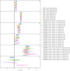 |
Fig. D.1 Comparison of RV mass estimates for various activity models and priors. |
In order to avoid biasing the final mass estimates for the combined RV + photodynamical fit, but still benefiting from the RV constraints, we selected from this analysis the FEN-RIR two modes, four harm, Matérn 1/2 activity model. Indeed, for the most model-sensitive planets (e, f, and g) this model exhibits large uncertainties on the mass posteriors and strong prior-sensitivity, which reflects the overall lack of constraint we have on these masses rather well. However, this does not mean that this an intrinsically better model for stellar activity. In particular, we noticed that the rotation period is not well constrained with this model as it reaches the upper bound of the prior interval. We stress here the need for additional RV measurements to better constrain the masses and activity model.
Appendix E Adding a planet in the chain
Here, we check whether additional planets in the resonant chain, on an external orbit to the known planet g, could either better explain the available data or invalidate the masses that we found for the six-planet solution. We considered a set of first- and second-order mean-motion resonances and computed what their orbital period should be to fit in the resonant chain. For each of these potential periods for planet h, we ran 10 fits of the individual transit timings shown in Figs. 4 and 5. Each of these fits were initialised as follow: the orbital parameters and masses of the planets c to g were set to the best fit of the photo-dynamical analysis, the mean longitude of planet h was randomly picked in the [0°,360°] range, the period was randomly picked in order to continue the chain with a super-period of 260 ± 20 days (see Eq.C.6 of L21). The expressions kh = eh cos ϖh and hh = eh sin ϖh were initially set at 3 10−4 and Mh /M was initially set to 6 10−7. The set of priors is identical to the ‘high-mass’ case described in Sect. 3.2. Once these fits converged, the best solution of each fit was used to initialise a joint photo-dynamical+RV fit, identical in all points to those presented in Sect. 3.2, only adding the additional planet.
In Fig. E.1, we show the best solution of each of these fits, as a function of the MMR near to the g-h pair, the mass of planet h, and the logprob of the solution. From these, we find that several resonances have similar probabilities, with the general trend that the larger Ph, the more massive mh. Such a degeneracy is well understood when considering the TTV induced at the super-period for nearly resonant pair of planets (e.g. Lithwick et al. 2012; Hadden & Lithwick 2016). However, there are additional arguments that could have allowed us to favour some solutions with respect to others. Indeed, small period ratios can also lead to short-term sawtooth-like TTVs known as chopping (Deck & Agol 2015, e.g.), that could better explain the TTVs of planet g. In addition, some of the tried periods for h are also close to significant MMR with planet f: for example, g and h close to a 3:2 or a 5:4 MMR implies that f and h are close to a 2 : 1 or a 5:3 MMR, which could also impact the overall goodness of the fit.
Our best solutions are for an additional planet between a 5/4 and 3/2 MMR with planet g, and masses of the order of 1MEarth or less. We would like to point out that the parameter space for this potential additional planet is much larger than the ones explored here; therefore, we cannot exclude that an additional more massive planet is orbiting TOI-178, especially if it is not in direct continuation of the resonant chain. Nonetheless, this preliminary study allows us to draw two conclusions: there are no obvious signals in the available data for an additional planet in the chain and the best fits of the available data with the additional planet do not significantly impact the derived mass for the known planets in the system. Indeed, we aggregated the mass of the planets b to g for the best fits of the configurations where the added planet has a period in either 5/4, 4/3, 7/5, or 3/2 MMR with planet g. These aggregated results are represented in cyan in the Fig. 9. As we can see, these aggregated masses remain close to the six-planet solution with the high-mass prior.
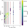 |
Fig. E.1 Best solutions of the joint photo–dynamical + RV fit when adding an hypothetical planet h near various MMR with respect to planet ɡ. |
References
- Acuña, L., Lopez, T. A., Morel, T., et al. 2022, A&A, 660, A102 [NASA ADS] [CrossRef] [EDP Sciences] [Google Scholar]
- Adibekyan, V., Sousa, S. G., Barros, S. C. C., et al. 2024, A&A, 683, A159 [NASA ADS] [CrossRef] [EDP Sciences] [Google Scholar]
- Ahrer, E., Queloz, D., Rajpaul, V. M., et al. 2021, MNRAS, 503, 1248 [NASA ADS] [CrossRef] [Google Scholar]
- Aigrain, S., Pont, F., & Zucker, S. 2012, MNRAS, 419, 3147 [NASA ADS] [CrossRef] [Google Scholar]
- Barbary, K. 2016, J. Open Source Softw., 1, 58 [Google Scholar]
- Benz, W., Broeg, C., Fortier, A., et al. 2021, Exp. Astron., 51, 109 [Google Scholar]
- Bertin, E., & Arnouts, S. 1996, A&AS, 117, 393 [NASA ADS] [CrossRef] [EDP Sciences] [Google Scholar]
- Bonfils, X., Astudillo-Defru, N., Díaz, R., et al. 2018, A&A, 613, A25 [NASA ADS] [CrossRef] [EDP Sciences] [Google Scholar]
- Boué, G., Oshagh, M., Montalto, M., & Santos, N. C. 2012, MNRAS, 422, L57 [NASA ADS] [Google Scholar]
- Brandeker, A., Heng, K., Lendl, M., et al. 2022, A&A, 659, A4 [Google Scholar]
- Bryant, E. M., Bayliss, D., McCormac, J., et al. 2020, MNRAS, 494, 5872 [Google Scholar]
- Cubillos, P., Erkaev, N. V., Juvan, I., et al. 2017, MNRAS, 466, 1868 [Google Scholar]
- Dai, F., Masuda, K., Beard, C., et al. 2023, AJ, 165, 33 [NASA ADS] [CrossRef] [Google Scholar]
- Deck, K. M., & Agol, E. 2015, ApJ, 802, 116 [NASA ADS] [CrossRef] [Google Scholar]
- Deck, K. M., & Agol, E. 2016, ApJ, 821, 96 [CrossRef] [Google Scholar]
- Deck, K. M., Agol, E., Holman, M. J., & Nesvorný, D. 2014, ApJ, 787, 132 [CrossRef] [Google Scholar]
- Deline, A., Hooton, M. J., Lendl, M., et al. 2022, A&A, 659, A74 [NASA ADS] [CrossRef] [EDP Sciences] [Google Scholar]
- Delisle, J. B., Hara, N., & Ségransan, D. 2020, A&A, 638, A95 [EDP Sciences] [Google Scholar]
- Delisle, J. B., Unger, N., Hara, N. C., & Ségransan, D. 2022, A&A, 659, A182 [NASA ADS] [CrossRef] [EDP Sciences] [Google Scholar]
- Delrez, L., Leleu, A., Brandeker, A., et al. 2023, A&A, 678, A200 [NASA ADS] [CrossRef] [EDP Sciences] [Google Scholar]
- Emsenhuber, A., Mordasini, C., Burn, R., et al. 2021, A&A, 656, A69 [NASA ADS] [CrossRef] [EDP Sciences] [Google Scholar]
- Fortier, A. Simon, A. E., Broeg, C., et al. 2024, A&A, 687, A302 [NASA ADS] [CrossRef] [EDP Sciences] [Google Scholar]
- Gaia Collaboration (Brown, A. G. A., et al.) 2018, A&A, 616, A1 [NASA ADS] [CrossRef] [EDP Sciences] [Google Scholar]
- Gaia Collaboration (Brown, A. G. A., et al.) 2021, A&A, 649, A1 [NASA ADS] [CrossRef] [EDP Sciences] [Google Scholar]
- Gillon, M., Triaud, A. H. M. J., Demory, B.-O., et al. 2017, Nature, 542, 456 [NASA ADS] [CrossRef] [Google Scholar]
- Goździewski, K., Migaszewski, C., Panichi, F., & Szuszkiewicz, E. 2016, MNRAS, 455, L104 [Google Scholar]
- Hadden, S., & Lithwick, Y. 2016, ApJ, 828, 44 [NASA ADS] [CrossRef] [Google Scholar]
- Hadden, S., & Lithwick, Y. 2017, AJ, 154, 5 [Google Scholar]
- Hara, N. C., & Delisle, J.-B. 2023, arXiv e-prints [arXiv:2304.08489] [Google Scholar]
- Hara, N. C., Boué, G., Laskar, J., Delisle, J. B., & Unger, N. 2019, MNRAS, 489, 738 [Google Scholar]
- Izidoro, A., Ogihara, M., Raymond, S. N., et al. 2017, MNRAS, 470, 1750 [Google Scholar]
- Izidoro, A., Schlichting, H. E., Isella, A., et al. 2022, ApJ, 939, L19 [NASA ADS] [CrossRef] [Google Scholar]
- Jenkins, J. M., Twicken, J. D., McCauliff, S., et al. 2016, SPIE Conf. Ser., 9913, 99133E [Google Scholar]
- Kipping, D. M. 2013, MNRAS, 434, L51 [Google Scholar]
- Kreidberg, L. 2015, PASP, 127, 1161 [Google Scholar]
- Leleu, A., Alibert, Y., Hara, N. C., et al. 2021a, A&A, 649, A26 [NASA ADS] [CrossRef] [EDP Sciences] [Google Scholar]
- Leleu, A., Chatel, G., Udry, S., et al. 2021b, A&A, 655, A66 [CrossRef] [Google Scholar]
- Leleu, A., Delisle, J. B., Udry, S., et al. 2023, A&A, 669, A117 [NASA ADS] [CrossRef] [EDP Sciences] [Google Scholar]
- Lendl, M., Anderson, D. R., Collier-Cameron, A., et al. 2012, A&A, 544, A72 [NASA ADS] [CrossRef] [EDP Sciences] [Google Scholar]
- Lithwick, Y., Xie, J., & Wu, Y. 2012, ApJ, 761, 122 [Google Scholar]
- Lopez, T. A., Barros, S. C. C., Santerne, A., et al. 2019, A&A, 631, A90 [NASA ADS] [CrossRef] [EDP Sciences] [Google Scholar]
- Luger, R., Sestovic, M., Kruse, E., et al. 2017, Nat. Astron., 1, 0129 [Google Scholar]
- Luque, R., Osborn, H. P., Leleu, A., et al. 2023, Nature, 623, 932 [NASA ADS] [CrossRef] [Google Scholar]
- MacDonald, M. G., Ragozzine, D., Fabrycky, D. C., et al. 2016, AJ, 152, 105 [Google Scholar]
- Millholland, S., Petigura, E., & Batygin, K. 2020, ApJ, 897, 7 [NASA ADS] [CrossRef] [Google Scholar]
- Mills, S. M., Fabrycky, D. C., Migaszewski, C., et al. 2016, Nature, 533, 509 [Google Scholar]
- Mills, S. M., & Mazeh, T. 2017, ApJ, 839, L8 [Google Scholar]
- Otegi, J. F., Bouchy, F., & Helled, R. 2020, A&A, 634, A43 [NASA ADS] [CrossRef] [EDP Sciences] [Google Scholar]
- Pepe, F., Cristiani, S., Rebolo, R., et al. 2021, A&A, 645, A96 [NASA ADS] [CrossRef] [EDP Sciences] [Google Scholar]
- Ragozzine, D., & Holman, M. J. 2010, ApJ, submitted [arXiv: 1006.3727] [Google Scholar]
- Rauer, H., Catala, C., Aerts, C., et al. 2014, Exp. Astron., 38, 249 [Google Scholar]
- Ricker, G. R., Winn, J. N., Vanderspek, R., et al. 2015, J. Astron. Telescopes Instrum. Syst., 1, 014003 [Google Scholar]
- Rivera, E. J., Laughlin, G., Butler, R. P., et al. 2010, ApJ, 719, 890 [Google Scholar]
- Skrutskie, M. F., Cutri, R. M., Stiening, R., et al. 2006, AJ, 131, 1163 [NASA ADS] [CrossRef] [Google Scholar]
- Smith, A. M. S., Eigmüller, P., Gurumoorthy, R., et al. 2020, Astron. Nachr., 341, 273 [Google Scholar]
- Smith, J. C., Stumpe, M. C., Van Cleve, J. E., et al. 2012, PASP, 124, 1000 [Google Scholar]
- Stumpe, M. C., Smith, J. C., Van Cleve, J. E., et al. 2012, PASP, 124, 985 [Google Scholar]
- Stumpe, M. C., Smith, J. C., Catanzarite, J. H., et al. 2014, PASP, 126, 100 [Google Scholar]
- Weiss, L. M., & Marcy, G. W. 2014, ApJ, 783, L6 [Google Scholar]
- Wheatley, P. J., West, R. G., Goad, M. R., et al. 2018, MNRAS, 475, 4476 [Google Scholar]
- Wright, E. L., Eisenhardt, P. R. M., Mainzer, A. K., et al. 2010, AJ, 140, 1868 [Google Scholar]
- Wu, Y., & Lithwick, Y. 2013, ApJ, 772, 74 [Google Scholar]
- Zeng, L., Sasselov, D. D., & Jacobsen, S. B. 2016, ApJ, 819, 127 [Google Scholar]
All Tables
All Figures
|
Fig. 1 Detrended light curves from CHEOPS as described in Sects. 2.1 and 3.3 The unbinned data are shown as blue points and the data from the 30 min bins are shown as green circles. The best fitting transit model for the system is shown in black; the associated parameter values are from the final posterior shown in Tables 2 and 3. Vertical lines indicate the planet that is transiting, unflagged transits are caused by planet b. Each line contains about six days of observation. Data published in L21 are indicated by a red upper line, the one published in D23 by an orange upper line, and new data by a green upper line. The raw and detrended data are available at the CDS. |
| In the text | |
|
Fig. 2 Detrended light curves from TESS as described in Sects. 2.2 and 3.3. The unbinned data are shown as blue points and the data from the 30 min bins are shown as red circles. The best fitting transit model for the system is shown in black; the associated parameter values are from the final posterior shown in Tables 2 and 3. Each line contains about 11 days of observation. The detrended data are available at the CDS. |
| In the text | |
|
Fig. 3 Detrended light curves from NGTS as described in Sects. 2.3 and 3.3. Data in 30 min bins are shown as purple circles. The best-fitting transit model for the system is shown in black; the associated parameter values are from the final posterior shown in Tables 2 and 3. The line contains about two days of observation, each visit containing the data taken by respectively 7, 4, 3, 4, 4, 4, 3, 4, and 5 of the NGTS telescopes. The unbinned data are not shown because the scatter is much larger than the than the flux range shown here. The raw and detrended data are available at the CDS. |
| In the text | |
|
Fig. 4 Transit timing variations observed for TOI-178 c, d and e. The filled area correspond to the 1σ posterior of the photo-dynamical fits presented in Sect. 3.2. The error bars show an estimation of the 1σ interval for the mid-transit timing of individual transits for each instrument, with transparency depending on the precision of the timings. See the text for more details. |
| In the text | |
|
Fig. 5 Mass-radius relationship of the TOI-178 planets (final posterior), compared with the super-Earth to Mini-Neptune populations for which the mass was derived through RV (Otegi et al. 2020) and TTVs (Hadden & Lithwick 2017; Leleu et al. 2023). The composition lines ‘terrestrial Earth-like’, in solid brown, and pure MgSiO3 ‘rocky’, in dashed brown, are taken from Zeng et al. (2016). |
| In the text | |
|
Fig. 6 Mass-radius relationship of the TOI-178 planets (final posterior), compared with the super-Earth to Mini-Neptune populations for which the mass was derived through RV (Otegi et al. 2020) and TTVs (Hadden & Lithwick 2017; Leleu et al. 2023). The composition lines ‘terrestrial Earth-like’, in solid brown, and pure MgSiO3 ‘rocky’, in dashed brown, are taken from Zeng et al. (2016). |
| In the text | |
|
Fig. 7 Mean density of the TOI-178 planets as a function of their equilibrium temperature. |
| In the text | |
|
Fig. 8 Three-sigma envelope of the evolution of the Laplace angles Ψ1, Ψ2, and Ψ3 over 1000 yr for the final posterior. |
| In the text | |
|
Fig. 9 Mass determinations for different datasets and choices of priors. In black: the posterior from the RV analysis with the FENRIR two modes – four harmonics – Matérn 1/2 model (see Appendix D). The blue posteriors are from the photo-dynamical model alone, while the green posteriors are from the joint photo-dynamical and RV fits. The ‘default’, ‘high-mass’, and ‘final’ set of priors are defined in Sect. 3.2. The cyan posterior synthesise the best fits of all our models with additional planets in the resonant chain, see Appendix E. The photodyn ‘final’ and photodyn+RV ‘final’ are the cases reported in Tables 2 and 3. |
| In the text | |
|
Fig. B.1 Detrended light curves from EulerCam as described in Sect. 2.4. The unbinned data are shown as blue points and the data from the 30 min bins are shown as purple circles. The best-fitting transit model for the system is shown in black. |
| In the text | |
|
Fig. D.1 Comparison of RV mass estimates for various activity models and priors. |
| In the text | |
|
Fig. E.1 Best solutions of the joint photo–dynamical + RV fit when adding an hypothetical planet h near various MMR with respect to planet ɡ. |
| In the text | |
Current usage metrics show cumulative count of Article Views (full-text article views including HTML views, PDF and ePub downloads, according to the available data) and Abstracts Views on Vision4Press platform.
Data correspond to usage on the plateform after 2015. The current usage metrics is available 48-96 hours after online publication and is updated daily on week days.
Initial download of the metrics may take a while.