| Issue |
A&A
Volume 668, December 2022
|
|
|---|---|---|
| Article Number | A162 | |
| Number of page(s) | 28 | |
| Section | Extragalactic astronomy | |
| DOI | https://doi.org/10.1051/0004-6361/202243600 | |
| Published online | 15 December 2022 | |
Constraining the multi-scale dark-matter distribution in CASSOWARY 31 with strong gravitational lensing and stellar dynamics⋆
1
Max-Planck-Institut für Astrophysik, Karl-Schwarzschild-Str. 1, 85748 Garching, Germany
e-mail: This email address is being protected from spambots. You need JavaScript enabled to view it.
2
Technische Universität München, Physik Department, James-Franck Str. 1, 85748 Garching, Germany
3
Academia Sinica Institute of Astronomy and Astrophysics (ASIAA), 11F of ASMAB, No. 1, Section 4, Roosevelt Road, Taipei 10617, Taiwan
4
Cosmic Dawn Center, Niels Bohr Institute, Univ. of Copenhagen, Jagtvej 128, 2200 Copenhagen, Denmark
5
Dipartimento di Fisica, Università degli Studi di Milano, Via Celoria 16, 20133 Milano, Italy
6
INAF-IASF Milano, Via A. Corti 12, 20133 Milano, Italy
Received:
21
March
2022
Accepted:
5
October
2022
Abstract
We study the inner structure of the group-scale lens CASSOWARY 31 (CSWA 31) by adopting both strong lensing and dynamical modeling. CSWA 31 is a peculiar lens system. The brightest group galaxy (BGG) is an ultra-massive elliptical galaxy at z = 0.683 with a weighted mean velocity dispersion of σ = 432 ± 31 km s−1. It is surrounded by group members and several lensed arcs probing up to ≃150 kpc in projection. Our results significantly improve on previous analyses of CSWA 31 thanks to the new HST imaging and MUSE integral-field spectroscopy. From the secure identification of five sets of multiple images and measurements of the spatially resolved stellar kinematics of the BGG, we conduct a detailed analysis of the multi-scale mass distribution using various modeling approaches, in both the single and multiple lens-plane scenarios. Our best-fit mass models reproduce the positions of multiple images and provide robust reconstructions for two background galaxies at z = 1.4869 and z = 2.763. Despite small variations related to the different sets of input constraints, the relative contributions from the BGG and group-scale halo are remarkably consistent in our three reference models, demonstrating the self-consistency between strong lensing analyses based on image position and extended image modeling. We find that the ultra-massive BGG dominates the projected total mass profiles within 20 kpc, while the group-scale halo dominates at larger radii. The total projected mass enclosed within Reff = 27.2 kpc is 1.10−0.04+0.02 × 10¹³ M⊙. We find that CSWA 31 is a peculiar fossil group, strongly dark-matter dominated toward the central region, and with a projected total mass profile similar to higher-mass cluster-scale halos. The total mass-density slope within the effective radius is shallower than isothermal, consistent with previous analyses of early-type galaxies in overdense environments.
Key words: gravitational lensing: strong / galaxies: elliptical and lenticular / cD / galaxies: groups: general / galaxies: kinematics and dynamics / galaxies: structure
Full Table B.1 is only available at the CDS via anonymous ftp to cdsarc.cds.unistra.fr (130.79.128.5) or via https://cdsarc.cds.unistra.fr/viz-bin/cat/J/A+A/668/A162
© The Authors 2022
 Open Access article, published by EDP Sciences, under the terms of the Creative Commons Attribution License (https://creativecommons.org/licenses/by/4.0), which permits unrestricted use, distribution, and reproduction in any medium, provided the original work is properly cited.
This article is published in open access under the Subscribe-to-Open model.
Open access funding provided by Max Planck Society.
1. Introduction
In the Λ cold-dark-matter (CDM) paradigm, dark-matter halos evolve and grow hierarchically by accretion of smaller halos (e.g., Subramanian et al. 2000), and higher-density environments collapse and form galaxies earlier. The evolution history of the most massive galaxies with M* > 1011 M⊙ is well described by this hierarchical model. This population formed on average earlier than lower-mass galaxies, during short bursts of intense star formation maintained over a few hundred megayears, which was followed by rapid quenching (e.g., Thomas et al. 2005; Pacifici et al. 2016; Tacchella et al. 2022). Large amounts of observations and simulations suggest that the main star formation episodes occurred at z > 2, and that active galactic nuclei are primarily responsible for the quenching phase (e.g., Springel et al. 2005; Croton et al. 2006); this leaves compact red quiescent galaxies at z ∼ 2 (e.g., Moster et al. 2020), which subsequently undergo dry mergers (e.g., Naab et al. 2007; Remus et al. 2013), grow in size (e.g., Naab et al. 2009; van der Wel et al. 2014), and form the massive elliptical galaxies in the local Universe. Each evolutionary process has a direct, traceable impact on the properties of the descendants observed at low redshift. For instance, higher-mass ellipticals are thought to have more violent merger histories, which lowers their stellar angular momentum compared to less massive counterparts (Emsellem et al. 2007). The properties of galaxies at the highest end of the mass distribution, with ultra-high stellar velocity dispersions (σ ∼ 500 km s−1), are particularly useful for further improving our understanding of this evolutionary sequence. At low redshifts, z ∼ 0, these systems are larger and redder than equivalents at lower masses (e.g., Bernardi et al. 2011). They are also extremely rare, and their precise number density can be related to key properties, such as the redshift of their main growth phase (e.g., Loeb & Peebles 2003).
On larger scales, the mass distribution of cluster-scale dark-matter halos has been extensively studied with various techniques, including galaxy kinematics, X-rays, and gravitational lensing. Detailed diagnostics have also been obtained for the baryonic and dark-matter content of massive ellipticals residing near the cores of such massive, dynamically relaxed clusters (e.g., Newman et al. 2013b,a). In addition, galaxy groups are the most common structures in the Universe and are believed to play a crucial role in the hierarchical formation of large-scale halos (e.g., Eke et al. 2004; Sommer-Larsen 2006). Despite successful searches in wide-field surveys (e.g., Belokurov et al. 2009; More et al. 2012), few galaxy groups have precise mass distribution measurements (Spiniello et al. 2011; Deason et al. 2013; Newman et al. 2015), which complicates the interpretation of the apparent diversity in their physical properties (e.g., Limousin et al. 2009a; Muñoz et al. 2013).
Standard CDM simulations predict universal mass-density profiles for dark-matter halos, independent of the total halo mass (Navarro et al. 1996, 1997). In reality, baryonic physics also plays a fundamental role, and the interplay between baryons and dark matter directly affects the total mass distributions. Gas cooling can result in the adiabatic contraction of dark-matter halos (Blumenthal et al. 1986), while, on the contrary, mergers and feedback from massive stars, supernovae, or active galactic nuclei can expand the dark-matter distributions (e.g., Nipoti et al. 2004; Pontzen & Governato 2012). Due to these competing processes, the inner mass-density slopes of dark-matter halos predicted by hydrodynamical simulations are either similar to the Navarro-Frenk-White (NFW) profile (e.g., Navarro et al. 1996; Schaller et al. 2015) or flatter (e.g., Martizzi et al. 2012), depending on the different prescriptions of feedback processes. Observational constraints on the halo properties can thus provide insights into the baryonic physics taking place during galaxy growth, and into their relative importance in setting the present-day dark-matter distributions.
Due to its sensitivity to all integrated mass along the line of sight, the strong gravitational lensing effect is very useful for robustly measuring mass distributions and exploring the relation between dark and luminous mass (e.g., Spiniello et al. 2011). The positions of multiple images can be used to calculate the deflection angles, and to determine the lens mass within the separation between observed images (i.e., within the Einstein radius, θE). Strong lensing studies have radically improved our understanding of the fundamental properties of galaxy and galaxy cluster dark-matter halos and subhalos (Vegetti et al. 2012). Since this effect is sensitive to the total mass on θE scales, generally on the order of the effective radius of the main foreground lens galaxy (e.g., Newman et al. 2015, and references therein), strong lensing is often complemented with stellar dynamics. The combination of strong lensing and spatially averaged stellar kinematics has tightly constrained the inner slope of the total mass-density profiles of isolated galaxies (Koopmans & Treu 2003; Treu & Koopmans 2004; Auger et al. 2009; Sonnenfeld et al. 2015) and that of massive ellipticals in overdense environments (e.g., Newman et al. 2013a) that act as deflectors. These probes did not reveal significant dark-matter contraction (e.g., Dutton & Treu 2014; Newman et al. 2015). For group- and cluster-scale lenses, these joint analyses have helped improve the mass model accuracies toward the central regions (e.g., Sand et al. 2008).
Combining strong lensing with spatially resolved stellar dynamics from integral-field-unit spectroscopy is particularly helpful for breaking the mass-sheet degeneracy (Falco et al. 1985), by constraining the amount of the mass sheet that is related to the main lens (e.g., Yıldırım et al. 2021). Combining these fine observational constraints with stellar population synthesis analyses is generally sufficient for disentangling the dark-matter and baryonic contributions to the total mass-density profiles. This leads to reliable measurements of the radial slopes of the dark-matter density profiles, which can be used to search for deviations from the standard NFW profile. Joint modeling of strong lensing and 2D stellar dynamics is relatively easy for galaxy groups or clusters in hydrostatic equilibrium, which are typically well de-blended and for which the stellar kinematics of the foreground lens have less source contamination.
In this work we present a detailed analysis of the inner mass structure of the group-scale lens CASSOWARY 31 (CSWA 31; see also Belokurov et al. 2009; Brewer et al. 2011; Stark et al. 2013). This strong gravitational lens reveals interesting perspectives that can be used to simultaneously constrain both the total and dark-matter mass distributions within a galaxy group at z = 0.683 and its ultra-massive central elliptical galaxy. CSWA 31 has a large Einstein radius of 70 kpc and shows several multiply imaged sources at various projected separations from the lens centroid (Grillo et al. 2013, and Fig. 1). In contrast to most group-scale lenses that have small image separations of ≤5″ (e.g., Auger et al. 2008; Limousin et al. 2009b; Newman et al. 2015), the peculiar configuration of CSWA 31 makes it well suited for characterizing the mass density slope of an extended group-scale halo beyond 100 kpc. In addition, combining strong lensing and stellar dynamics modeling of CSWA 31 has the potential to constrain the inner slope of the total mass-density profile and to robustly distinguish between the relative contributions from the central galaxy and the group-scale halo within 10 kpc (e.g., van de Ven et al. 2010; Barnabè et al. 2012). This system can therefore be used as a testbed to unveil the inner structure of massive ellipticals and their host galaxy groups at intermediate redshift. We use new high-quality imaging from the Hubble Space Telescope (HST) and integral-field spectroscopy from the Multi-Unit Spectroscopic Explorer (MUSE; Bacon et al. 2014) to extend previous studies of CSWA 31 with more detailed parametrizations of the lens mass distribution and to develop novel methods for separating the multi-scale components.
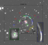 |
Fig. 1. HST/WFC3 image of CSWA 31 and its surrounding environment in the F160W band. The orientation is marked by the black arrows in the bottom-right of the figure, and the ruler indicates a physical scale of 150 kpc in the main lens plane at z = 0.683. The large black box marks the total 1′ × 1′ coverage of MUSE observations. The small 8″ × 8″ black box in the center shows the field of view considered for the dynamical analysis of the main lens galaxy, and the x′ and y′ arrows show the orientation adopted for the kinematic maps (see Sect. 5). The sets of spectroscopically confirmed multiple images used in our analysis are marked with circles, with a different color for each set. The image sets S0 and S1 are bright knots from the same spiral galaxy at z = 1.4869, with a zoomed-in image of S0(d) in the left inset. The right inset shows the bright arc from source galaxy S3 at z = 2.763. The multiple images of source 4 (S4) are identified with MUSE and undetected in this HST image. |
The paper is organized as follows. In Sect. 2 we briefly summarize previous analyses of CSWA 31, and we present the new imaging and spectroscopic observations, as well as redshift measurements. In Sect. 3 we provide an overview of the formalism of our strong lensing and stellar dynamics modeling, as well as the numerical methods for inferring the best-fit parameters of the mass models. We present the lensing-only models of CSWA 31 in Sect. 4 and the joint lensing and dynamics modeling in Sect. 5. In Sect. 6 we compare the best-fit mass models from previous sections, and we put the results in context with other group- and cluster-scale lenses in the literature. In Sect. 7 we summarize our results and give an outlook on general studies of galaxy groups. Throughout this work we assume H0 = 70 km s−1 Mpc−1, Ωm = 0.3, and ΩΛ = 0.7. Hence, 1″ corresponds to 7.08 kpc at the lens redshift of z = 0.683.
2. Observations
The CSWA 31 lens system was discovered in Sloan Digital Sky Survey (SDSS) imaging as part of the Cambridge And Sloan Survey Of Wide ARcs in the skY (CASSOWARY; Belokurov et al. 2009), and was analyzed by Brewer et al. (2011), Stark et al. (2013), and Grillo et al. (2013, hereafter G13). The main lens galaxy of CSWA 31 is located in the group center and will be referred to as the brightest group galaxy (BGG). This is an early-type galaxy at z = 0.683 with a very high stellar mass of about 3 × 10¹² M⊙ and an aperture-averaged stellar velocity dispersion of 450 ± 80 km s−1 from SDSS (G13), which suggests it is among the rarest ultra-massive elliptical galaxies at these redshifts (with comoving number densities ≲10−8 Mpc−3, Loeb & Peebles 2003). The BGG is surrounded by group members and by giant lensed arcs formed by a face-on spiral at z = 1.487. G13 used Gemini/GMOS imaging and VLT/X-shooter spectroscopy to characterize the lens total and stellar-to-total mass profiles, based on the four multiple images of this main background source1. They measured a total mass of 4 × 10¹³ M⊙ projected within the Einstein radius and found that CSWA 31 is strongly dark-matter dominated in its center. Subsequently, Leethochawalit et al. (2016) took advantage of the lensing magnifications to characterize the spatially resolved kinematics and gas-phase metallicity gradients within the background spiral galaxy based on Keck/OSIRIS integral-field spectroscopy. We present here the additional observables inferred from our new HST and MUSE data set.
2.1. HST/WFC3 imaging
We used high-resolution HST optical and near-infrared imaging in filters F438W and F160W over a field of view of ∼2′ × 2′ to resolve galaxies and lensed sources, and perform lens mass modeling. One-orbit exposures of ∼2400 s were taken in each of the two filters with the Wide Field Camera 3 in November 2018 (program GO-15253; PI: Cañameras). We re-drizzled the individual exposures with the DrizzlePac software package (Fruchter et al. 2010) with optimal sampling, using final_pixfrac = 0.6 and 0.033″ pix−1 in F438W, and final_pixfrac = 0.8 and 0.066″ pix−1 in F160W. We used flat fields from the WFC3/IR monitoring campaigns to correct the small regions with decreased sensitivity in the F160W image. After correcting the astrometry, both images were saved on the same grid using Scamp and SWarp (Bertin 2006, 2010). We built point spread function (PSF) models by stacking four bright, unsaturated stars in the field, and measured PSF of 0.09″ and 0.19″ in the reduced F438W and F160W images, respectively, about five times lower than ancillary ground-based imaging.
The WFC3 F160W image shown in Fig. 1 not only probes the bulk of the old stellar populations in the BGG, group members and other galaxies in the field, but also provides a sharp, high signal-to-noise ratio (S/N) image of the main lensed arc formed by the face-on spiral galaxy at z = 1.487, and detections of several additional faint arcs. The F438W band provides color information to help determine whether or not observed images are associated with the same background source. Sets of multiple images and selection of group members are then robustly confirmed with spectroscopy. Positions adopted in the modeling in Sects. 4 and 5 are given in pixel units, using a reference coordinate at RA = 9:21:19.349 and Dec = +18:10:52.50 (bottom-left corner of Fig. 1), and orientation following the (x, y) arrows in Fig. 1.
2.2. VLT/MUSE spectroscopy
This work uses MUSE data from program 0104.A-0830(A) (PI: Cañameras) in order to resolve the stellar velocity dispersion profile of the primary lens up to ∼10 kpc, and to secure the identification and redshift measurements of group members and multiple image candidates. Observations were carried out in December 2019 and January 2020, with seeing ≤1″, clear sky conditions, and airmass < 1.6, with the MUSE wide-field mode corresponding to 1′ × 1′ field of view and 0.2″ pix−1 spatial sampling. We divided the observations into five individual observation blocks (OBs), applying a dithering pattern and 90° rotations between each OB, and obtained a total on-source exposure time of 5 h.
The data were reduced with the standard MUSE pipeline (Weilbacher et al. 2014) following the procedure described in Caminha et al. (2019). After correcting raw exposures for the bias, flat fields and illumination frames, we applied wavelength and flux calibrations. The individual exposures were then combined into a stacked data cube. We optimized the sky subtraction with the ZAP software (Soto et al. 2016), and defined the astrometry with respect to the HST F160W image. The reduced MUSE data cube has a PSF full width at half maximum of 0.69″. The instrument spectral resolution ranging from 1770 at 4800 Å to 3590 at 9300 Å, and the constant 1.25 Å pix−1 sampling, make these data well-suited to reliably measure the lens stellar dynamics. In addition, the MUSE pointing shown in Fig. 1 encloses all arcs and multiple image candidates detected with HST, as well as the majority of galaxies within the foreground group covering about 450 kpc.
To measure source redshifts, we followed Caminha et al. (2017, 2019) by analyzing the MUSE data cube using two different methods. First, we extracted the spectra at the positions of sources detected in the HST F160W image, using circular or optimized apertures depending on the source morphology. Second, we adapted the line search for sources with faint stellar continuum, undetected with HST, by extracting sources from a continuum-subtracted MUSE data cube. We then inspected both the spatially averaged spectra and the spectra extracted along two perpendicular directions, in order to identify emission lines, absorption lines, or continuum breaks and measure redshifts. We also fitted templates to sources with bright stellar continuum to help infer their redshift. Finally, we assigned a quality flag (QF) to each object, by ranking the reliability of redshift measurements as QF = 3 (secure), 2 (likely), or 1 (not reliable). Redshifts inferred from single, but unambiguous line identifications such as the [OII] doublet are considered secure. We obtained a total of 121 spectroscopic redshifts with QF ≥ 2 (see Appendix B).
2.3. Identification of multiple images
From the MUSE redshift catalog, we identified a total of five sets of multiple images listed in Table 1 and shown in Fig. 1. The face-on spiral galaxy at z = 1.4869 forming the bright arc is labeled as S0. Its four counter-images were the only ones spectroscopically confirmed prior to our analysis, with S0(b) and S0(d) secured by Keck/DEIMOS and MMT spectroscopy in Stark et al. (2013), and S0(a) and S0(c) confirmed by G13. In addition to S0 centered on the galaxy bulge, we also find a doubly imaged blue star-forming clump within the disk of this spiral galaxy, which we mark as S1. The second brightest arc labeled S3(b) has a single counter-image S3(a), both at z = 2.763. The proposed counter images of S3(b) – that is, the radial image located between S0(a) and S0(d) and the tangentially elongated object southwest of S5(d) from G13 – have spectroscopic redshifts of z = 0.3296 (QF = 3) and z = 1.359 (QF = 3), respectively, and are therefore ruled out by our MUSE data. Moreover, the two merging images S5(a) and S5(b) of the faint, diffuse external arc have reliable redshifts of z = 4.205, as well as their counter-image S5(c). The redshift of S5(d) from a blind template fitting is z = 4.203 (QF = 3), but with higher uncertainties than for S5(a-c) due to the lower spectrum S/N (see Fig. B.1). In addition, its color is consistent with images S5(a-c), and its observed position and morphology match the expectations from simple lens models based on image families S1-S3. We therefore included S5(d) as a fourth counter-image and fixed its redshift to z = 4.205. We checked that the (F438W − F160W) aperture colors measured with SExtractor (Bertin & Arnouts 1996) are within 1σ uncertainties for all multiple images in these sets (Table 1).
Position, spectroscopic redshift, and (F438W − F160W) color for the BGG and multiple images used in the modeling.
Lastly, S4 is identified exclusively with MUSE, without stellar continuum counterpart in HST. We obtained three multiple image candidates with single emission lines interpreted as Lyα at z = 3.4280. Since the positions of S4(a-c) are consistent with the predictions of our strong lensing models based on the other image families, we also included this set in the analysis.
These five multiple-image families in the field of CSWA 31 provide a number of secure strong lensing constraints comparable with studies of galaxy clusters based on similarly deep HST images (shallower than for the Frontier Field program; e.g., Jauzac et al. 2019; Mahler et al. 2019; Caminha et al. 2019; Rescigno et al. 2020; Richard et al. 2021). This rich data set allows us to adopt a parametrized composite mass model to investigate the inner structure of this complex lens system in more details than previous analyses. It should be noted that we measured the positions of multiple images from our highest resolution F160W image with SExtractor, except for S4, which is only detected with MUSE and thus has a larger positional uncertainty. The MUSE 1D spectra are shown in the Appendix B together with the spectral features used to identify multiple image families.
2.4. Properties of the foreground galaxy group
To select group members we relied on our best redshift estimate of z = 0.6828 for the BGG. We then selected all galaxies from the MUSE spectroscopic catalog located within ±3000 km s−1 with respect to the rest frame of the BGG and we obtained a total of 46 group members (see Fig. 2). We measured robust redshifts for members down to K(AB) ∼ 23 mag, about 3 mag fainter than L* galaxies at z ∼ 0.7 (see, e.g., Fassbender et al. 2011), and we checked that their number is not sensitive to the exact velocity thresholds. The lack of spectroscopic coverage toward the group outer regions prevents us from inferring the total halo mass, M200, based on the line-of-sight velocities of satellite galaxies at 1−3 Mpc from the lens center (see, e.g., Munari et al. 2013; Deason et al. 2013). The MUSE data nonetheless cover the entire core region and provides valuable constraints to include the group members in our composite lens mass models.
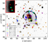 |
Fig. 2. HST F160W image showing the BGG (red star), group members (orange stars), the reference galaxy used in the scaling relations (purple star), and sets of multiple images (circles). We modeled the emission of group members 1, 2, 3, 4, and 5 (cyan filled stars) together with the BGG in order to minimize light contamination on the nearby lensed arcs. Given the significant contribution of group members 1, 2, 6, and 7 to the light deflection angles, their Einstein radius were optimized separately. The image positions predicted by models Img-SP (L) and Img-MP (L) are marked by plus and cross symbols, respectively. Similarly, the mean weighted source positions reconstructed by models Img-SP (L) and Img-MP (L) are indicated with bold plus and cross symbols, respectively. The solid purple line shows the critical curve of model Img-SP (L) with regards to S0. The upper-left inset zooms in on the 3.6″ × 4.9″ rectangle to highlight the intrinsic positions of S0, S1, and S5 in both models. The solid purple line shows the critical curve of model Img-MP(L) for z = 1.487, the redshift of S0. The critical curves of other reference models are shown in Appendix E. |
The number of members within the central 1′ × 1′ and their corrected isophotal magnitudes measured in F160W with SExtractor further suggest that CSWA 31 is a rich galaxy group. Sparse clusters in the Abell catalog have a minimum of 30 members within a magnitude range between m3 and m3+2, where m3 is the magnitude of the third brightest member, while confirmed members of CSWA 31 span ≃5.6 mag, and only 19 are between m3 and m3+2. This suggests that CSWA 31 is not rich enough to meet the criteria from Abell. While additional members could lie outside the MUSE field of view and within the 2.5 Mpc radius corresponding to the compactness criteria from the Abell catalog, our HST photometry indicates that their number is much lower than toward the core.
CSWA 31 has been identified as one of the most distant candidate fossil systems by G13 and Johnson et al. (2018), in which case the extreme brightness of the BGG (21 mag arcsec−2 in r-band) would result from the past, slow accretion of all surrounding group members of intermediate masses (e.g., Khosroshahi et al. 2007). Fossil systems are considered as the final evolutionary stages of galaxy groups and Johnson et al. (2018) showed that, due to their elevated halo concentration, they are more efficient gravitational lenses than standard groups. The positions and brightnesses of group members spectroscopically confirmed with our new observations further suggest that CSWA 31 meets the fossil criteria from Jones et al. (2003). However, additional data are still needed to confirm that CSWA 31 is a progenitor of fossil groups seen in the local Universe. In particular, weak lensing constraints would help measure R200 and, while G13 reported a non-detection in X-rays from the ROSAT All-Sky Survey (RASS), deeper X-ray observations would help characterize the hot gas and dynamical state of CSWA 31.
We estimated the stellar mass of the BGG by modeling its spectral energy distribution (SED) with the Code Investigating GAlaxy Emission (CIGALE; Burgarella et al. 2005; Noll et al. 2009; Boquien et al. 2019). We used a grid of models based on Bruzual & Charlot (2003) single stellar population templates, assuming delayed star formation histories with ages between 0.5 and 8 Gyr. We used the modified Charlot & Fall (2000) extinction law, a Salpeter (1955) stellar initial mass function, and a solar metallicity (see also Conroy et al. 2013; Gallazzi et al. 2014) to fit the Pan-STARRS and HST photometry. Varying the dust extinction during the fit results in elevated AV ≳ 3 mag, essentially due to the lack of data points at infrared wavelengths. Assuming low dust extinction, as expected for massive ellipticals, gives a comparable fit while changing the stellar mass by 0.1 dex, and results in M* = (1.6 ± 0.4)×1012 M⊙ (see Fig. A.1). This estimate is lower but consistent with the value reported in G13.
3. Methodology
In this work, we used the Gravitational Lens Efficient Explorer (GLEE; Suyu & Halkola 2010; Suyu et al. 2012) software to model the mass components and surface brightness of galaxies by adopting parametrized mass and light profiles. We also used Gravitational Lensing and Dynamics (GLaD, Chirivì et al. 2020; Yıldırım et al. 2020), an extension of GLEE to perform a joint lensing and stellar dynamics modeling. GLaD adopts the projected second-order velocity moment along the line of sight,  , as inputs for Jeans anisotropic modeling (JAM; Cappellari 2008) to estimate the dynamical parameters of galaxies. In Sect. 3.1, we present the strong lensing formalism in the single- and multi-plane scenarios (see also Blandford & Narayan 1986; Schneider 2006). In Sect. 3.2, we have a short overview of the dynamical modeling approach (see also Binney & Tremaine 1987; Cappellari 2008; Barnabè et al. 2012; Yıldırım et al. 2020). In Sect. 3.3, we summarize the sampling methods to infer the best-fitting parameters.
3.1. Strong lensing
In the general relativity paradigm, a light ray can be deflected differentially due to the deformation of space-time along the line of sight induced by massive clumps with potential ψ,
 (1)
(1)
where κ is the dimensionless surface mass density, so-called convergence, and θ is the lensed source position. The potential connects to the scaled deflection angle α via α = ∇ψ. This leads to the following relation between κ and α:
 (2)
(2)
The mass distributions of the deflectors are modeled using different parametrizations of the convergence κ. Firstly, we used the softened power-law elliptical mass distribution (SPEMD; Barkana 1998) with κ defined in Cartesian coordinates (x1, x2) as follows, for a source at redshift zs = ∞,
 (3)
(3)
where the amplitude E is related to the Einstein radius θE via
 (4)
(4)
The first two terms in Eq. (3) depict the elliptical shape of the mass distribution, q is the axis ratio, rcore is the core radius, and γ is the power-law slope, which is related to the 3D density slope γ′ as γ′ = 2γ + 1, where  . This corresponds to an isothermal mass profile for γ = 0.5 and γ′ = 2. Secondly, we also use the truncated dual pseudo-isothermal elliptical mass distribution (dPIE; Elíasdóttir et al. 2007; Suyu & Halkola 2010) defined as
 (5)
(5)
where rtr is the truncation radius, rcore is the core radius, θE is the Einstein radius, given rtr = ∞ and rcore = 0 and Rem is the elliptical mass radius related to the ellipticity e = (1 + q)/(1 + q), where q is the axis ratio, defined as
 (6)
(6)
The corresponding 3D density distribution is proportional to r−2 for rcore ≤ r < rtr, and drops as r−4 for r > rtr. This truncation can represent the tidal stripping of galaxy halos in dense group or cluster environments (e.g., Limousin et al. 2009a; Suyu & Halkola 2010). Both SPEMD and dPIE can be rotated by a position angle θPA to account for the orientation of the mass distribution.
Thirdly, we introduce a constant external shear to account for the tidal stretching from neighbor galaxies. The lens potential for an external shear is parametrized in polar coordinates as
 (7)
(7)
where γext represents the strength of the external shear, and the shear angle θext represents the stretching orientation of the images. The shear center can be selected arbitrarily because it corresponds to an unobservable constant shift in the source plane. The external shear does not contribute to the surface mass density of the lens due to the vanishing external convergence κext from  , but it affects the shape of the observed images. For shear position angles θext = 0° and θext = 90°, lensed image configurations are elongated along the horizontal and vertical axes, respectively.
We adopted the dPIE profile to model the total mass of individual lens galaxies such as the BGG and group members, and the SPEMD profile to model the dark-matter component in the group-halo and BGG. Further details on the mass parameters are given in Sects. 4 and 5.2.
To optimize the unknown parameters η (i.e., the parameters introduced in mass profiles) in the adopted κ, we used the observed multiple images as constraints via Eq. (2), the geometry relation between the background source position β, and the observed image positions θ. In the single plane, the light rays from the background source are deflected by a single deflector (lens), yielding the lens equation
 (8)
(8)
with the scaled deflection angle α expressed as
 (9)
(9)
where Dds, Ds, Dd are the angular diameter distances between lens and source, between observer and source, and between observer and lens, respectively. In the multi-plane scenario, the lens equation, Eq. (8), can be modified as follows to account for multiple deflections produced by a sequence of n − 1 lenses distributed at different redshifts along the line of sight:
 (10)
(10)
In this equation, θn represents the position of the light ray in the nth plane, namely the source plane, with respect to the position of the light ray in the first observed lens plane θ1. θi is the image of the lensed source in the ith plane,  is the deflection angle on the ith plane, Din is the angular diameter distance between the ith plane and nth plane, and Dn is the angular diameter distance between the observer and nth plane. The case n = 2 corresponds to a single lens plane and Eq. (10) reduces to Eq. (8).
For each lens model, we can calculate the lens surface mass density Σ via κ with a single lens plane, for a given source at redshift zs,
 (11)
(11)
with the critical surface mass density Σcrit defined as
 (12)
(12)
This results in a definition of Σ depending only on Dd:
 (13)
(13)
We can then deduce the total mass enclosed within a radial distance R from the defined lens center with
 (14)
(14)
For multiple lens planes, Σ becomes an effective surface mass density, corresponding to the gradient of the total deflection angle via Eq. (3) that includes the contributions from all lenses along the line of sight. In that case, while the quantity inferred from Eq. (14) is not physical, it remains a good approximation for the enclosed mass.
3.2. Stellar dynamics
Stellar dynamics can capture the inner mass distribution within the effective radius Reff by connecting the line-of-sight velocity, v, and the velocity dispersion, σ, to the mass potential. This probe is widely used in complement to strong gravitational lensing (e.g., van de Ven et al. 2010; Barnabè et al. 2012; Yıldırım et al. 2020).
The motion of a group of stars within a galaxy can be characterized by the Collisionless Boltzmann equation with phase-space density f(x, v) at the position x with velocity v,
 (15)
(15)
which describes stars embedded in a gravitational field ψD following phase-space density conservation. The phase-space density is not accessible for distant galaxies, and we can only extract the velocities along the line of sight, v, and velocity dispersions, σ. To properly adopt the Collisionless Boltzmann equation, we therefore multiply velocities vR, vz, vϕ with Eq. (15) and integrate over all velocity space in cylindrical coordinates (R, z, ϕ). Assuming the alignment of an axisymmetric velocity ellipsoid with the cylindrical coordinate system, we obtain the following two equations, so-called axisymmetric Jeans equation,
 (16)
(16)
 (17)
(17)
where the orbital anisotropy parameter,  , presents a flattening in the meridional plane. We used a simplified notation of the second-order velocity moments
  ,
,
 (18)
(18)
where λ is the intrinsic luminosity density of galaxies. The second-order velocity moments are projected onto the plane of sky with an inclination i, to obtain  as Eq. (20), which can be related with the measurable quantities v and σ as follows:
 (19)
(19)
![Mathematical equation: $$ \begin{aligned} &+\overline{v_z^2} \mathrm{cos}^2i]~\mathrm{d}z\prime = v^2 + \sigma ^2 = V^2_{\rm rms}. \end{aligned} $$](/articles/aa/full_html/2022/12/aa43600-22/aa43600-22-eq28.gif) (20)
(20)
In this equation,  is expressed in cartesian coordinates (x′,y′,z′), where x′ and y′ presents the coordinates on the plane of sky and z′ describes the direction along the line of sight. The observed surface brightness of galaxies μ is the intrinsic surface brightness λ projected onto the plane of sky with an inclination i. Both the surface brightnesses (λ, μ) and the potential ψD can be modeled with multiple 2D Gaussians. We can thus connect these components via the stellar mass-to-light luminosity ratio Γ = M*/L. The terms λ and ψD can be incorporated into the Jeans equations and Eq. (20) to infer the dynamical parameters of galaxies (βz, i, Γ) given the measured second-order moments Vrms.
3.3. Best-fitting parameters
Both GLEE and GLaD use parametrized profiles and the Bayesian method to infer the values of the free model parameters. The posterior distributions of parameters P(η|d) describe the probability of obtaining a set of parameters η given the data set d as
 (21)
(21)
where P(η) is the prior on the parameters, which we assumed to be uniform, except for the centroids of mass components that have Gaussian priors. P(d) is the evidence, and ℒ(d|η) is the likelihood presenting the probability that the measurements d are produced by η. It is related to the squared residuals χ2 between the modeled and observed data,
 (22)
(22)
and the maximal likelihood therefore corresponds to the minimal χ2. We note that η refers to parameters in the mass and light profiles in our lensing-only models, and to the mass, light, and dynamical parameters in our joint lensing and dynamical analysis. The input data d depend on the configuration of each model and will be introduced specifically in Sects. 4 and 5. The posterior distributions of parameters P(η|d), given the data d are sampled with Markov chain Monte Carlo (MCMC) methods, using the emcee ensemble sampling algorithm by Foreman-Mackey et al. (2013). We ensured that the MCMC chains converge to steady state distributions, which indicates that the posterior probability distribution functions (PDFs) of the free parameters are well sampled and can be used to find the maximum of P(η|d).
In practice, we computed the models in two steps. First of all, we assumed realistic measurement errors on the observed quantities, which are, depending on the model, the centroid positions of multiple images, the position of pixels along the extended arcs, the lens stellar kinematics per spatial bin, or a combination thereof. We tested various mass parametrizations, ran the parameter optimization for each model, and compared the output reduced χ2 per degrees of freedom (d.o.f.). The concrete χ2 form depending on the model will be introduced in Sects. 4 and 5. Secondly, a range of good mass models with low χ2/d.o.f. were selected and we ran MCMC chains to sample the posterior PDFs. For this step, we slightly increased the measurement errors in order to obtain a rescaled χ2/d.o.f. = 1 and to infer the realistic parameter uncertainties listed together with the best-fit and marginalized values in Sects. 4 and 5. This approach allowed for a direct comparison of models based on different sets of constraints or different mass parametrizations. Rescaling the χ2 also accounts for mass perturbations not represented by the parametric descriptions of the lens potentials, such as line-of-sight components, or asymmetries in the main lens plane.
4. Mass modeling with strong lensing
To begin, we modeled the total mass of the deflectors via the strong lensing technique. In Sect. 4.1 we present the modeling of the lens light distribution, which serves as an input for the lens mass modeling. In Sect. 4.2 we constrain the total mass of the deflectors using the observed centroid positions of multiple images, both in the single-plane and multi-plane scenarios. To describe the dense environment of CSWA 31, we first adopted composite mass models with a single lens plane at redshift z = 0.6828 to account for the BGG, group members, the extended group-scale dark-matter halo, and a constant external shear. Given that light rays from the most distant lensed source can be deflected by other mass components near the line of sight, we then conducted multi-plane modeling with a secondary lens at redshift z = 1.4869. In Sect. 4.3, we present the modeling of the extended lensed source emission. Since the surface brightness is conserved between the source and observed images, we exploited the information from the pixel light intensities of extended lensed arcs in order to refine the best-fit mass models obtained from image positions.
4.1. Lens light modeling
We characterized the stellar continuum emission of the brightest foreground galaxies using the high-S/N F160W image. Modeling the light distribution of the BGG and other individual lens galaxies helps us define priors for several parameters of our lens models such as the centroids, axis ratios, and position angles of the galaxy-scale mass components. In addition, some group members are in close proximity to the lensed arcs, and we need to subtract their light contamination before conducting the extended image modeling in Sect. 5.3. Lastly, light modeling is particularly useful to distinguish the baryonic mass component of the BGG from dark matter in Sect. 5.
For each galaxy, we adopted one or multiple light profiles to model the surface brightness of each galaxy Ij in pixel j, by convolving with our PSF model in F160W band described in Sect. 2.1. We minimized the sum of the offsets between the predicted Ij ⊗ PSF, and the observed Iobs, j intensities in Np pixels with the following χ2:
 (23)
(23)
where the term σtotal includes background noise σbg and Poisson noise σPoisson as
 (24)
(24)
We simultaneously fitted the light distribution of the BGG and of five group members indicated in Fig. 2 that are in proximity to the lensed images. Such early-type, elliptical galaxies are well described by Sérsic profiles (Sérsic 1963). Figure 2 shows that the light emission of the BGG has a prominent diffuse component toward the south, and we adopted two Sérsic profiles with different central positions to account for this asymmetry. To describe the surface brightness of the other five group members with symmetrical isophotes, we used a Sérsic and a Gaussian profile with linked centroids. During the fitting process, we masked out the flux from lensed arcs and other neighboring galaxies over the field.
The best-fit parameters 1σ (68% CI) uncertainties for the light distribution of the BGG shown in the Table 2 are the most probable values inferred from the peak of the joint posterior PDFs. We also listed the median and the 16th and 84th percentiles of the 1D marginalized posterior PDFs. The best-fit model and its normalized residual are shown in Fig. 3. We obtained  , which corresponds to a reduced
  . The BGG dominates the contributions to the global
  for the six galaxies, due to the strong central residual and slight under-fitting toward the south, and fitting only the BGG while masking other group members in the field leads to
  . We note that the central residuals are restricted to ≲0.5″ and do not alter the extended image modeling. The under-fitting of the BGG toward the south highlights the limitations of our parametrization with symmetrical Sérsic profiles, and does not significantly impact the surface brightness distribution of the lensed arcs. The emission from group members shows lower residuals (Fig. 3).
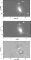 |
Fig. 3. Best-fit model for the light distribution of the BGG and five nearby group members. From top to bottom: observed HST F160W band image, the best-fit model, and the normalized residuals in the range −7σ to 7σ. In all three images, the constant areas are the masks covering the lensed arcs and other objects in the field. The panels cover a field of view of 36″ × 22″ and are oriented in the same way as in Fig. 1, with north approximately toward the bottom. |
Best-fit and marginalized values with 1σ uncertainties for the near-infrared light modeling of the BGG in CSWA 31.
The first Sérsic profile in Table 2 accounts for the majority of the light emission from the BGG and we used its effective radius, Reff = 27.2 kpc at z = 0.6828, as measurement of the BGG size. This value is consistent with the effective radius fitted with a single Sérsic component, with the estimate from G13, and matches the size of BGGs at lower-redshift (z ∼ 0.2 − 0.45; Newman et al. 2015). We also used the best-fit position, axis ratio q and position angle θPA of the first Sérsic profile to constrain the BGG mass potential in our lens models. As explained below, other group members in the field are described with simple spherical potentials fixed at the positions from our light modeling.
4.2. Image position modeling
Strong gravitational lensing provides tight constraints on the lens mass distribution over radial ranges where the lensed arcs emerge. In this section we present the lens mass modeling inferred from the peak positions of multiple images belonging to the six families presented in Sect. 2.3 and plotted in Fig. 2. These sets provided us with 36 constraints to build composite models of the lens mass distribution, and to fit a large number of parameters in the convergence κ. The cumulative 1D lens mass profiles were then computed via Eq. (14). After deducing the best-fit lens mass parameters, the intrinsic source positions retraced from each multiple image are expected to agree with each other. In practice, since residuals in our mass modeling introduces small shifts, we defined the intrinsic source position as the mean source position weighted by the magnification μ of the observed images.
4.2.1. Lens mass parametrization
To characterize the structure of CSWA 31 in detail and to separate the lens mass components on various scales, we used composite models including the BGG, group members, the dark-matter group halo, and a constant external shear for the dense environment around CSWA 31. Strong gravitational lensing and dynamical modeling of early-type galaxies have shown that their total mass density profiles are well described by nearly isothermal power-law models (Koopmans et al. 2006; Gavazzi et al. 2007; Barnabè et al. 2009; Sonnenfeld et al. 2013; Tortora et al. 2014; Cappellari et al. 2015). Consequently, we modeled the total mass of the BGG and group members with dPIE profiles. Due to the limited number of multiple images, we scaled the total mass of the group members to a member selected arbitrarily, the so-called reference galaxy, as commonly done in galaxy-cluster lens modeling (e.g., Richard et al. 2010; Grillo et al. 2016; Limousin et al. 2016; Caminha et al. 2019; Chirivì et al. 2018) and we assumed circular symmetry. Given that such galaxies lie on the fundamental plane, we assumed that their Einstein radius and truncation radius scale with their F160W band luminosities. We followed Grillo et al. (2015) and Chirivì et al. (2018) in setting the following scaling relations to ensure that total mass-to-light ratios follow the tilt of the fundamental plane
 (25)
(25)
where Li and Lref are the F160W band luminosities of group member i and reference galaxy, respectively. The mass of an arbitrary group member i in CSWA 31 can be characterized by θE, ref and rtr, ref, once we determined the light ratio Li/Lref between the group member i and the reference galaxy and plugged it into the scaling relation 25. Thus, the mass of an individual group member is regarded as a multiple of the reference galaxy. Instead of varying the individual mass profiles, we optimized the reference galaxy mass in terms of θE, ref and rtr, ref to reduce the number of optimized parameters.
Foreground galaxies in proximity to the lensed images have a significant impact on the deflection angle α of the light rays from the corresponding background source. To account for this, we fitted separately the Einstein radius θE of four group members (1, 2, 6, and 7 in Fig. 2). The truncation radius of these galaxies is comparable to their half-mass radius and typically larger than the scales where the multiple images emerge. Consequently, we do not expect good constraints on rtr from the strong lensing configuration of CSWA 31 and we kept their truncation radius rtr in the scaling relations. We note that the aforementioned group members 3, 4, 5 induce significant light contamination to the main arc, but their surface brightness in the F160W band suggests lower masses and hence smaller contributions to the light deflection. For both BGG and group members, we assumed vanishing core radii since the strong lensing constraints do not cover the inner region of these individual galaxies.
We chose the SPEMD to model the mass distribution of the underlying extended dark-matter halo. This profile has more flexibility than the NFW profile thanks to its variable surface mass-density slope γ. We imposed flat priors on the parameters of the group-scale SPEMD and, in particular, we restricted its core radius to rcore, GH = 6″ − 14″. This range is motivated by recent strong lensing studies of extended dark-matter halos (e.g., Richard et al. 2021) and using strict boundaries allowed us to exclude models with arbitrarily large SPEMD cores. In addition, other group members located out of the MUSE field of view are not part of the scaling relations. A constant external shear component was added to account for the tidal stretching to the multiple images induced by such neighboring galaxies and by other mass components in CSWA 31.
We then ran MCMC chains to sample the maximal posterior probability P (see Eq. (21)), which is presented in terms of priors and  defined as
 (26)
(26)
where Nset is the number of multiple image families (see Fig. 2), Nimg, i is the number of individual counter-images in family i,  is the observed position of image j from multiple image family i,
  is the predicted image position, and σj, i is the position uncertainty of image j from multiple image family i.
We introduced elliptical positional uncertainties for the multiple images with high magnification that form the extended arcs, and circular uncertainties for S0(d) and image set S4 (Table 1). For sets S0, S1 and S2, we fixed the positional uncertainties along the elliptical minor and major axes to one and two HST image pixels, respectively, with major axes oriented along the direction of the arcs. For S3(b), we used four pixels as positional error along the major axis given the diffuse morphology of this extended arc, and for S4 identified by MUSE, we also used larger errors (e.g., three pixels) due to the larger MUSE PSF. For set S5, we used larger errors along both elliptical axes because S5 is fainter than other image sets detected with HST. After comparing the χ2 of various models, we rescaled these uncertainties by a factor of three in order to get a  /d.o.f. = 1. This allowed us to derive realistic parameter uncertainties, to directly compare the models with different structures (e.g., single-plane versus multi-plane), and to account for the simplistic dark-matter halo parametrizations, the number of possible missing group members out of the field of MUSE, the possible asymmetries in the lens mass distribution, and other perturbations along the line of sight. Such perturbations include six galaxies detected with MUSE at z = 1.357, which are all distant from the BGG centroid and should therefore only produce a small perturbation in the lens mass modeling.
4.2.2. Results in the single- and multi-plane scenarios
First, we followed the single-plane modeling approach, considering that the light rays from all background sources are deflected once by the BGG, group members and extended dark-matter halo located within a single lens plane at redshift z = 0.6828, with negligible deflections from mass perturbations along the line of sight. An MCMC chain was run to minimize the  in Eq. (26), with the
  terms computed in the single-plane framework. Figure 2 shows that the observed positions of multiple images are well reproduced by this model, which we refer to as Img-SP (L), given the best-fit parameters η of the mass profiles and the best-fit source positions β. Before rescaling the reduced
  we obtained
  /d.o.f. = 14.76. The best-fit and marginalized parameter values with 1σ uncertainties are displayed in Table 3.
Best-fit and marginalized values with 1σ uncertainties for the parameters of our lensing-only models based on image positions, in the single-plane (Img-SP (L)) and multi-plane scenarios (Img-MP (L)).
Second, we expanded this model to multiple lens planes, as done in strong lens modeling of galaxies (e.g., Gavazzi et al. 2008) or galaxy clusters (e.g., D’Aloisio et al. 2014; Bayliss et al. 2014; Chirivì et al. 2018) to account for the line-of-sight mass distribution and reduce the offset between observed and predicted image positions. In CSWA 31, we observe that the weighted mean source positions of S0, S1 and S5 inferred from model Img-SP (L) have small projected separations (see Fig. 2). This means that light rays from S5 can be deflected substantially by S0 (and S1, which belongs to the same galaxy) in addition to the main lens potential at z = 0.6828. We thus conducted the multi-plane mass modeling with S0 as a secondary lens at z = 1.4869, using a spherical isothermal mass profile fixed at the best-fit source position from Img-SP (L). Other sources forming sets S2, S3, and S4 reside in between the observer and S5, but their weighted mean positions are poorly aligned with each other and with S5, and we therefore ignored their impact on the total deflection angles. We obtained  /d.o.f. = 8.87 for this model called Img-MP (L), which is a significant improvement with respect to Img-SP (L). The results are also listed in Table 3. The best-fit value of the Einstein radius of S0, θE, S0, is 4.36″, which indicates a non-negligible perturbation along the line of sight.
Model Img-MP (L) has smaller rms for all sets of multiple images compared to Img-SP (L), given the best-fit parameters η of the mass profiles and the source positions β. Multiple images of sources 0, 1, 2, 5 are accurately reproduced, within 0.2″ and 0.3″ on average in Img-MP (L) and Img-SP (L), respectively (see Fig. 2). Sets S3 and S4 show larger uncertainties and can be reproduced within 0.5″ in Img-MP (L) and within 0.6″ in Img-SP (L). Models Img-SP (L) and Img-MP(L) predict a third image for set S3, falling in the vicinity of the BGG centroid (see Fig. 2). This image is however de-magnified by factors μ = 5 × 10⁻⁵ and μ = 0.8 in Img-SP (L) and Img-MP (L), respectively, and it is not detected in our imaging and spectroscopic data due to strong blending with the BGG.
We conducted several tests to quantify the impact of the adopted parametrization and the selection of image constraints on the model results. Firstly, we added all group members, including those near the lensed arcs, to the scaling relations in order to model their mass exclusively via the parameters θE, ref and rtr, ref. Secondly, we tested the influence of the core radius of the group-scale halo on the overall analysis by fixing this parameter to rcore, GH = 0 during optimization. These two tests substantially increased the  /d.o.f., because the output mass models were unable to recover the image positions of the most distant source galaxy (S5) at z = 4.205. Lastly, S4 shows the largest offset between the predicted and observed image positions, and we determined the influence of S4 on the best-fit parameters by deriving new models excluding this set of multiple images. We found that the resulting best-fit parameters were within 1σ uncertainties compared to Img-SP (L) and Img-MP (L), and we therefore kept S4 as constraints in our models.
The marginalized parameter values given in Table 3 and the PDFs shown in Appendix C indicate that most parameters are constrained with similar precision for our two models, and consistent within 2σ. The values of θE are listed for sources at redshift z = ∞. After rescaling to the correct source redshifts, we obtained an Einstein radius for the BGG θE, BGG of about 3″ for z = 1.4869. This is comparable with Reff obtained in the lens light modeling and consistent with the range of θE, BGG measured for group-scale lenses in Newman et al. (2015). In contrast, we observe larger angular separations approaching ∼10″ for multiple images of S0 in the HST F160W frame. These separations are closer to the best-fit θE, GH for z = 1.4869 in both models and therefore likely primarily caused by the extended dark-matter halo. In addition, we find that some best-fit parameter values are more physical in model Img-MP (L), such as θE, ref = 0.44″, which converges to zero in model Img-SP (L). The core of the group-scale halo is more extended in model Img-SP (L), with a best-fit value approaching the prior upper limit, and which would diverge to unrealistically large cores rcore, GH ≫ 14″ for broader priors. For these reasons, and given that Img-MP (L) reproduces the image positions slightly better than Img-SP (L), we chose Img-MP (L) as the reference lens model based on image positions.
4.3. Extended image modeling
Most lensed background sources detected in our HST image exhibit extended morphologies. Moreover, the bright extended arc from image set S3 at z = 2.763 is diffuse and, contrary to source S0, the lack of structure introduces large uncertainties in our image position modeling of S3. To account for the source surface brightness distributions and to better constrain our mass models, we conducted the extended image modeling of CSWA 31 with GLEE. Given the surface brightness conservation I(θ) = I(β), the software reconstructs I(β) on a grid of pixels in the source plane, and then maps I(β) back to the image plane via the lens equation to obtain the predicted image morphology I(θ). We optimized the lens mass parameters by minimizing the offset between the predicted light intensity  and the observed light intensity dj in each pixel j of the extended arcs and foreground lens galaxies included in the fit. This is identical to minimizing
 (27)
(27)
where d includes the contributions of the lens galaxies and multiple images as d = dlens + dimage. The light intensity is written to a vector with length Nd, equal to the number of pixels from our F160W image included in the fit. CD is the image covariance matrix (Suyu et al. 2006) with diagonal terms only,
 (28)
(28)
where σtotal,j is derived from Eq. (23), N is the number of pixels. CD presents the noise correlation between adjacent pixels on the image plane, induced by charge transfer and drizzling. In this work, we adopt a robust assumption that the noise is uncorrelated in observed data for simplicity.
We modeled the extended images of sources S0 and S3, which have the highest S/N in our HST images, using their surface distribution in the F160W band. Source S5 at redshift z = 4.205 forms a fainter arc toward the outskirts of CSWA 31 and its S/N is insufficient to perform an extended image modeling. We kept the same parametrization of the foreground lens mass potential and, following our results in Sect. 4.2, we focused on the multi-plane scenario with a secondary lens at z = 1.4869. We fitted the light intensity of pixels forming the extended arcs from sets S0 and S3, which corresponds to ∼18 000 and ∼3000 pixels, respectively. In addition, we also included the positions of other multiple images in sets S2, S4, and S5 as constraints. Hence, we ran MCMC chains to minimize a combination of Eqs. (26) and (27) as follows:
 (29)
(29)
Our first model Esr2-MP (L) has a  before rescaling and fits the multiple images of S0 very well. This model however significantly over-fits the northern portion of the compact image S3 (a) in set S3 (see the left column of Fig. D.1). The counterimage of this region corresponds to the southern end of the extended arc S3(b), where the stellar continuum has a lower surface brightness. This faint and diffuse region extends up to image S0(c) and since it lacks a spectroscopic redshift from MUSE, the separation between the northern end of arc S0(c) and the southern end of S3(b) is ambiguous. Given the unverified redshift and the strong normalized residuals, it is also possible that this diffuse area is associated with a separate source instead of S3 at z = 2.763. To test, we ran a second model, Esr2-MPtest (L), based on an alternative mask focusing on the bright portion of the arc (see the right column of Fig. D.1). To account for the uncertainties in the mask design, we boosted the uncertainties at the mask boundary where the faint and bright regions blend with each other. This second model Esr2-MPtest (L) improves the fit of the counterimage of S3 and results in a lower χesr, img = 2.7 × 10⁴. The centroid, clumps and spiral arms of multiple images of S0 are well reproduced by both models despite the strong tangential distortions, as highlighted by the residuals in Fig. 4 for Esr2-MPtest (L). In both models, S0 and S3 are also well reconstructed on the source plane.
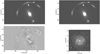 |
Fig. 4. Surface brightness reconstruction of source S0 at redshift z = 1.4869 from the best-fit model Esr2-MPtest (L). Two nearby group members are included in the modeling, while other objects within the gray regions are masked out. We show the observed HST F160W image over a field of view of 36″ × 22″ (top left), the best-fit model of the main arc, BGG and group members (top right), the normalized residual (bottom left) in the range −7σ to 7σ, and the source-plane reconstruction of S0 over a field of 2.1″ × 2.1″ (bottom right). The arc is well fitted and does not show significant residuals in the image plane. S0 has a clear spiral shape in the source plane. It is well reconstructed in all our lens models, with an intrinsic morphology consistent with our reference model Esr2-MPtest (L). |
The best-fit and marginalized parameter values of these two mass models are given in Table 4. Some of the parameters – θPA, GH, rcore, GH, γGH, rtr, BGG, and θE, 6 – differ by > 3σ between Esr2-MP (L) and Esr2-MPtest (L) and others are consistent within 3σ uncertainties. All parameters remain consistent with the 1σ contours from our image position reference model Img-MP (L). The strongest variation concerns the best-fit Einstein radius of S0 in the secondary lens plane, which decreases from 4.36″ in Img-MP (L) to ≃1.7″ in our extended image models. As mentioned above, Esr2-MP (L) and Esr2-MPtest (L) fit the image positions of other lensed sources (S2, S4, S5) together with the surface brightness distribution of S0 and S3. The constraints from these image positions are nonetheless overwhelmed by the constraints from the pixel intensities on the extended arcs. This effect explains the deviations in the best-fit values of Tables 3 and 4. Due to this weighting, both extended image models also lead to larger offsets between the observed and predicted positions of images in sets S2, S4, and S5, which are on average ≃0.9″. In the end, we chose the model Esr2-MPtest (L) with lower  and minor residuals as our reference lens model based on image morphologies.
Best-fit and marginalized values with 1σ uncertainties for the parameters of our lensing-only models based on the extended surface brightness distribution of sources S0 and S3 and on the positions of multiple images from other sets.
5. Mass modeling with strong lensing and stellar dynamics
Our constraints on the mass distribution of CSWA 31 can be significantly improved toward the lens center by jointly modeling the strong lensing observables with the lens stellar dynamics. In this section we use the spatially resolved kinematics of the BGG as additional information to constrain the mass components within the inner few kiloparsecs. In Sect. 5.1, we describe the extraction of stellar kinematics from the MUSE data cube. In Sect. 5.2, we present a joint dynamics and strong lens modeling assuming a parametrization identical to our previous models. In Sect. 5.3, we attempt to separate the total dark-matter contribution in CSWA 31 from the baryonic mass components inferred from the near-infrared surface brightness of galaxies.
5.1. Stellar kinematics of the BGG
We used the 2D spectra over a central 8″ × 8″ field of view extracted from our MUSE data cube (see Fig. 1) in order to measure the spatially resolved stellar kinematics of the BGG, namely the line-of-sight velocities, v, and the projected stellar velocity dispersions σ. We extensively tested the estimation of stellar kinematics from spectra with various S/N, and found that velocity dispersions tend to be overestimated for low and moderate S/N, in particular for massive early-type galaxies with broader absorption lines (Cañameras et al., in prep.). To optimize the S/N, we first binned the cube in the spectral dimension to a wavelength resolution of 3.75 Å pix−1. We then conducted Voronoi tessellations (Cappellari & Copin 2003) of the MUSE data cube to obtain a binned map with adequate S/N while preserving sufficient spatial information. We used a target S/N of 35 per spectral bin over the 3800−4400 Å rest-frame range where the main absorption lines emerge. This threshold ensures robust measurements for the BGG (see also Yıldırım et al. 2021) and results in a total of 17 resolution elements.
The kinematic information was extracted with spectral fitting, using the Penalized PiXel-Fitting (pPXF) method (Cappellari & Emsellem 2004). We selected a subset of the 105 stellar templates from the National Optical Astronomy Observatory library (Valdes et al. 2004), by focusing on G, K, and M spectral classes to match the typical stellar populations of early-type galaxies. These stellar templates cover a wavelength range from 3465 Å to 9469 Å, with an intrinsic spectral resolution of 1.35 Å, sufficient to fit the MUSE data. The spectra in each bin were fitted in the rest-frame range 3600−5100 Å with pPXF, to obtain v, σ, and the Gauss-Hermite moments of the line-of-sight velocity distributions h3 and h4. Firstly, we followed an iterative method to calibrate the BGG redshift in order to get unbiased line-of-sight velocities. We derived the best-fit redshifts for the 17 bins with pPXF, used the mean value to update the BGG redshift, and repeated the fitting procedure until the mean value stayed within < 10−6. The final BGG redshift is z = 0.6828. Secondly, we fixed the redshift to estimate the best-fit values of v, σ, h3, and h4 per bin together with their 1σ uncertainties. Six bins toward the galaxy outskirts do not meet our target S/N and have significantly larger parameter uncertainties. We focused on the 11 remaining bins within the central 2″ × 2″ to obtain reliable stellar kinematics for our joint lensing and dynamical modeling.
The maps of the best-fit v, σ, and second velocity moments  are shown in Fig. 5 for the 11 bins. We obtained the 1σ uncertainties σVrms of each bin l using
 (30)
(30)
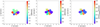 |
Fig. 5. Spatially resolved stellar kinematics of the BGG in 11 Voronoi bins with sufficient S/N extracted over a 8″ × 8″ field of view. The maps show the line-of-sight velocities v (left), the projected velocity dispersions, σ (middle), and the second velocity moments, Vrms (right). The orientation of the figure differs from the previous figures. The x′ axis points to the north and is aligned with the major axis of the BGG, while the y′ axis points to the west. Note that the spectrum shown in Fig. 6 corresponds to the central resolution element. |
where δv (≃25 km s−1) and δσ (≃30 km s−1) are the 1σ uncertainties of the line-of-sight velocities and velocity dispersions, respectively, obtained from pPXF. Figure 6 illustrates the quality of our fits. The main absorption lines that drive the stellar kinematic estimates, namely the Ca H and K lines at 3935 Å and 3970 Å, the G-band feature at 4305 Å, and Hβ at 4863 Å, are correctly fitted in all bins, as well as the highly prominent 4000 Å discontinuity. The BGG does not show significant rotation, as also found for the majority of massive early types in the local Universe (e.g., Emsellem et al. 2007), and σ varies between 380 and 500 km s−1. The Vrms map shows higher values along the minor axis of the BGG (y′ direction) and lower values along the major axis (x′ direction) with significant scatter. We note that due to stellar orbital anisotropies, the 2D projected Vrms can vary as a function of galactocentric radius, even for intrinsically constant velocity dispersions and total density profile slopes in 3D.
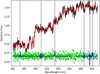 |
Fig. 6. Example of spectral fitting with pPXF for one resolution element in our binned data cube (the central bin in Fig. 5). The black and red lines show the observed spectrum normalized to unity and the best-fit stellar template, respectively. The green symbols at the bottom are the fit residuals, and the blue lines with gray-shaded regions show positions of gas emission lines masked during the fit. The most prominent spectral features used for the fit are the Ca H and K lines at 3935 Å and 3970 Å in the rest frame, the continuum break at 4000 Å, the G-band feature at 4305 Å, and the Hβ line at 4863 Å. Such high-S/N spectra are used to extract robust stellar kinematics for the BGG out to ≃0.5 Reff (see Fig. 5). |
We extensively checked our measurements to exclude systematic biases that would drastically affect the JAM outputs (e.g., Yıldırım et al. 2020). Varying the bias parameter in the range from 0 to 1 does not affect the values of v and σ, and we therefore fixed this parameter to the default value 0. Likewise, the polynomial order for continuum corrections has a minor influence on the results. In addition, we tested whether possible residuals in the subtraction of skylines falling at 3744.325 Å and 4305.407 Å in the rest frame of the BGG can impact the fitting (see Sect. 2). Masking out a few spectral bins around each skyline would cut the blue tail of the G-band absorption feature and would bias the stellar kinematics, with an unphysical average velocity dispersion of 650 km s−1. Alternatively, excluding the entire G-band feature leads to v and σ values consistent with the results inferred from the entire wavelength range. We therefore used the full MUSE spectra to derive our final results, assuming negligible residuals from the skyline subtraction.
The radial profile of Vrms is plotted in Fig. 7 and the σ profile of the BGG is essentially similar. The variations within ≲8 kpc are consistent with a flat radial profile given the 1σ errors. These results are in agreement with the lack of significant stellar velocity dispersion gradients in the majority of BGGs at z < 0.5 analyzed by Newman et al. (2015), and with the stellar kinematics of other individual early-type galaxies (e.g., the Cosmic Horseshoe at z = 0.44, Spiniello et al. 2011; Schuldt et al. 2019). At lower redshifts, Veale et al. (2018) obtained σ radial profiles for local early-type galaxies with M* > 4 × 10¹¹ M⊙ from the MASSIVE survey. They find a majority of negative gradients within the central few kiloparsecs and logarithmic slopes ranging between −0.2 and 0. In addition, Veale et al. (2018) detect a higher fraction of positive σ gradients in the highest-mass bin ≃1012 M⊙, but only for the outer 10−25 kpc radial range, which we cannot probe due to limited S/N in the MUSE data. Finally, from the best-fit stellar kinematics, we obtain a luminosity-weighted average velocity dispersion of the BGG of  km s−1, consistent with the value
  km s−1 previously measured by G13 from lower-S/N SDSS spectroscopy. The elevated
  confirms that the BGG is an ultra-massive early-type galaxy (Loeb & Peebles 2003).
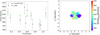 |
Fig. 7. Modeled stellar kinematics of the BGG. Left: Vrms radial profile predicted by the joint lensing and dynamical modeling Img-MP (L/D) (green triangles) from the most-probable model compared to the Vrms measured over the 11 Voronoi bins and their 1σ uncertainties (gray points). The radial position of each resolution element is defined with respect to the BGG centroid. The observed Vrms are consistent with a flat profile, and predicted values are within the 1σ ranges in most bins. Right: predicted Vrms map from model Img-MP (L/D), showing that this model does not fully recover the angular structure of Vrms in Fig. 5. |
5.2. Comparing joint and lensing-only models
The combination of strong lensing and stellar kinematic data has been proven highly successful in constraining the total mass-density slope and dark-matter fraction of galaxy-scale lenses (e.g., Koopmans & Treu 2003; Treu & Koopmans 2004; Auger et al. 2009; Sonnenfeld et al. 2015; Shajib et al. 2021). In CSWA 31, the six sets of multiple images provide direct constraints on the large-scale mass distribution, while the innermost image S4(b) falls around 20 kpc from the BGG center. The spatially resolved MUSE kinematics covering the central 8 kpc in 11 bins are thus expected to improve our diagnostics significantly. To test whether or not the joint modeling gives consistent results while breaking parameter degeneracies, we derived a first model based on the same configuration as our image position reference model Img-MP (L). This ensures similar contributions from lensing and dynamics to the total χ2 defined as
 (31)
(31)
Combining the stellar kinematics with extended arc surface brightness would on the other hand minimize the contribution of the kinematic data, with a χ2 dominated by the larger number of pixels on the extended arcs. For this reason, we did not attempt a comparison to Esr2-MPtest (L).
We used the GLaD software (Chirivì et al. 2020; Yıldırım et al. 2020) based on the JAM formalism presented in Cappellari & Copin (2003) and Cappellari (2008). This approach relies on the solutions of the Jeans equations in axisymmetric geometry, which is more flexible than assuming spherical Jeans models (e.g., Chen et al. 2021; Birrer & Treu 2021). In short, the code takes the 2D surface brightness and surface mass density maps from the lensing-only model, and de-projects these maps using multi-Gaussian expansions (MGEs) in order to infer analytical descriptions of the gravitational potentials, and to predict the second-order velocity moments Vrms. GLaD minimizes the χ2 in Eq. (31) by sampling the parameter space and iterating the lensing and dynamical modeling sequentially. For CSWA 31, we used flat priors on the orbital anisotropy parameter βz, between −0.8 and 0.8 and on the inclination angle i, between 80° and 90°. βz presents the intersection shape of the velocity ellipsoid on the meridional plane (vR, vz). When βz = 0, the ellipsoid is isotropic on (vR, vz), indicating the intersection shape is everywhere circle, when βz deviates from 0, the ellipsoid becomes anisotropic, stretching into an oblate (βz > 0) or prolate (βz < 0) (Cappellari et al. 2007). The angle i presents the way real galaxies are projected onto the observed plane; for example, a galaxy observed edge-on will have i = 90°. The MGE only included the dPIE describing the BGG given the negligible contributions of the group-scale halo to the inner κ. We ran an MCMC chain to infer βz, i, and lens-mass parameters.
The best-fit model Img-MP (L/D) has a χ2/d.o.f. = 5.22 before rescaling, lower than our lens models based on image positions, and it can reproduce the positions of multiple images of sets S0, S1, S2, and S5 within in average 0.2″, similarly to model Img-MP (L). The modeled positions of images in sets S4 and S5 are within 0.5″. The best-fit and marginalized parameter values of Img-MP (L/D) are shown in Table 5. The deprojection of the surface brightness via the inclination angle i to obtain the intrinsic luminosity density is not unique, implying that i is usually poorly constrained and degenerate with anisotropy βz. This effect explains the lack of constraints on the dynamical parameters of the BGG. On the other hand, parameters describing the mass profiles are consistent with the values in Table 3.
Best-fit and marginalized values with 1σ uncertainties for model Img-MP (L/D) based on joint constraints from strong lensing and stellar dynamics.
Model Img-MP (L/D) has a  and fits the MUSE stellar kinematics relatively well. Figure 7 shows that the predicted Vrms are within the measured 1σ ranges in most bins. However, the predictions do not fully recover the angular structure in the 2D map and underestimate Vrms along the BGG minor axis. We postulate that this discrepancy could be due to small asymmetries in the mass distribution of the BGG in CSWA 31, which would contradict the axisymmetry assumptions in GLaD. We indeed note that the near-infrared light emission of the BGG shows a south–north asymmetry, which could also be present in the underlying mass distribution. In fact, our reference lensing-only models suggest that the group-halo mass center is offset from the BGG mass center by ≃16.2 kpc, and the best-fit group-halo axis ratio is q ∼ 0.8. Given the small, but non-negligible contribution of the group-halo SPEMD within Rkin < 8 kpc, these properties induce a small asymmetry in the modeled mass distribution at the inner region covered by the stellar kinematic data. For these reasons, the properties of the BGG could approach the intrinsic limitations of JAM. Nonetheless, the overall good agreement between the predicted and observed radial profile of Vrms (Fig. 7, left panel) suggests adequate reconstruction of the lens mass distribution.
5.3. Separating the baryonic and dark-matter components
While keeping these limitations in mind, we attempted to disentangle the baryonic and dark-matter components in the BGG to constrain the overall dark-matter mass distribution in CSWA 31 (from the group-scale halo and BGG). G13 analyzed the ROSAT X-ray emission toward CSWA31, excluding significant hot gas emission from the intergalactic medium over 150 kpc around the BGG. For this reason, we assumed that stellar mass dominates the total baryonic mass budget within the radial ranges under consideration, and we modeled this component by scaling the near-infrared surface brightness distribution with a stellar mass-to-light ratio Γ. We reproduced the light modeling of the BGG with two Chameleon profiles (e.g., Dutton et al. 2011; Maller et al. 2000; Suyu et al. 2014), which can be related to pseudo-isothermal elliptical mass distributions (PIEMDs) to ease the calculation of lensing quantities, while mimicking the two Sérsic profiles in Table 2. These Chameleon profiles fit the BGG surface brightness equally well as in Fig. 3, with a  , only slightly higher than with Sérsic profiles (
 ). The analytical structure of each Chameleon profile I(x, y) given in Appendix A is equivalent to two PIEMDs with different core radii, such that the baryonic surface mass density can be defined as
 (32)
(32)
We kept the same configuration as Img-MP (L/D), except that we modeled the baryonic and dark-matter components of the BGG with four PIEMDs and a non-cored SPEMD, respectively, instead of a single dPIE. For simplicity, we used a single, spatially constant stellar mass-to-light ratio Γ to scale these PIEMDs, despite the mass-to-light radial gradients detected in samples of massive galaxies with independent constraints on the dark-matter density profiles (e.g., Sonnenfeld et al. 2018). We fixed the SPEMD profile of the BGG to the centroid position of the best-fit Chameleon profiles, and used the same parametrizations and priors as before for the group halo, group members, external shear, and S0 at z = 1.487.
The best-fit model Img-MP (L&D) can recover the measured Vrms within 1σ uncertainties similarly to model Img-MP (L/D), and can reproduce the positions of multiple images of S0, S1, S2, and S3 in average within 0.2″, and within 0.6″ for sets S4 and S5. The parameter Γ is relatively well constrained, to  , while the anisotropy βz, and inclination angle i are poorly constrained for the reasons given in Sect. 5.2. Moreover, other mass components are not strongly affected by the new parametrization for the BGG, and the best-fit profiles remain stable with respect to our previous models.
6. Model comparison and discussion
In Sect. 6.1, we compare the results from our lensing-only reference models based on image position (Img-MP (L)), and extended light (Esr2-MPtest(L)) reconstructions, and from our joint strong lensing and dynamical modeling (Img-MP (L/D)). In Sect. 6.2, we present the robust separation between the total mass of BGG and extended group halo and, in Sect. 6.3, we compute the slope of the total mass-density profile and we compare with the literature. Then, in Sect. 6.4, we disentangle the baryonic component within BGG from dark matter using model Img-MP (L&D), and we compare the resulting baryonic fraction with the SED analysis.
6.1. Constraints on the mass parameters
To test the consistency between models and probe parameter degeneracies, we plot in Fig. 8 the posterior PDFs for the parameters describing the BGG, extended group-scale halo, and secondary lens S0 at z = 1.487. The marginalized PDFs indicate that mass parameters are much better constrained for Esr2-MPtest (L), due to the large number of constraints from the lensed source morphologies. While the best-fit values of θE, GH, rcore, GH, and θE, S0 differ from the other two models, the joint PDFs remain consistent with Img-MP (L) and Img-MP (L/D).
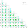 |
Fig. 8. Joint posterior PDFs for our three reference models, corresponding to the lensing-only models based on image positions (Img-MP (L), purple contours) and on extended surface brightness distributions (Esr2-MPtest (L), cyan contours), and to the joint modeling with strong lensing and dynamics (Img-MP (L/D), green contours). We focus on the most important mass parameters that describe the BGG and the extended group-scale halo. The three shaded areas on the joint PDFs show the 68.3%, 95.4%, and 99.7% credible regions. The 1D histograms show the marginalized PDFs for the selected mass parameters, and the vertical lines mark the 1σ confidence intervals. The model based on extended image fitting has narrower contours due to the large number of constraints from the lensed source morphologies. |
For the lensing-only models, we notice that the Einstein radius of the group-scale dark-matter halo θE, GH, and rtr, BGG and rE, S0 are less constrained in Img-MP (L) due to the joint contributions from the BGG, group-scale halo, and mass perturbations along the line of sight. θE, GH is larger for smaller BGG truncation radii rtr, BGG, and for smaller θE, S0. The slope of the group-halo SPEMD, γGH, is strongly degenerate with its core radius rcore, GH. While such parameter degeneracies usually complicate the separation of the central galaxy and host dark-matter halo in group-scale lenses (e.g., More et al. 2012), they have a lower impact for CSWA 31 (see Sect. 6.2). In particular, including extended arcs helps break these degeneracies since the additional constraints from S0 and S3 cover the same ranges as the 1D marginalized PDFs for θE, GH and rtr, BGG in Img-MP (L). We nonetheless note that the best-fit parameters of Esr2-MPtest (L) are likely slightly biased to the values optimizing the reconstruction of S0, which is more extended in the image plane. For the joint model Img-MP (L/D), the additional constraints from the BGG stellar kinematics only make the marginalized PDF of θE, BGG in Fig. 8 slightly narrower than Img-MP (L), others are comparable with Img-MP (L). The best fit and marginalized parameter values do not vary significantly between both models, and the parameter degeneracies are not completely broken in Img-MP (L/D), likely due to the large uncertainties in our stellar kinematics measurements (see Fig. 7). We expect that increasing the number of resolution elements with sufficient S/N, and using broader spectral coverage to decrease the errors on v and σ would improve the constraints from the joint modeling.
These results do not motivate the inclusion of a secondary extended mass component, as done for merging galaxy clusters (e.g., Lagattuta et al. 2017; Mahler et al. 2018), further suggesting that CSWA 31 is an isolated galaxy group. We note that the reference models discussed in this section are resulting from an extensive exploration of the parametrization of the foreground gravitational potential. Other choices of mass profiles, such as a NFW for the group-scale halo, significantly degrade the fit.
6.2. Contributions from the BGG and extended group-halo
We computed the cumulative projected mass profiles as a function of radial separation from the BGG light center for the main components in CSWA 31, namely the BGG and extended group-scale halo, and the results are shown in Fig. 9 for our three reference models. Other mass components with minor contributions to the cumulative mass profiles are ignored. The radial distributions are broadly consistent with each other in the range 20−150 kpc covered by multiple images of background sources. In particular, over this radial range, the total mass distributions are in excellent agreement with the mass model of G13 constrained exclusively from S0 marked by pink solid line with 1σ uncertainties in Fig. 9, but with much smaller 1σ uncertainties due to the additional constraints in our analysis. The group halo, and total masses are consistent with each other in our three mass models in the range 20−100 kpc where the brightest lensed images of S0 and S3 emerge, despite the small differences seen in Fig. 8 for γGH, the power-law slope of the group-halo SPEMD. The BGG mass from model Img-MP (L/D) is overall slightly lower but still comparable with other two reference models within 1σ uncertainties, which is induced by the smaller fitting values of θE, BGG in Img-MP (L/D). The total enclosed masses are broadly similar to the virial masses inferred by Muñoz et al. (2013) for strong-lensing galaxy groups at similar redshifts as CSWA 31. The masses enclosed within REin, S0 ∼ 70 kpc are  ,
,  , and
, and  for the BGG, group-halo, and all components, respectively, in model Esr2-MPtest (L).
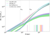 |
Fig. 9. Cumulative mass profiles as a function of radial separation from the BGG center, for the BGG (dot-dashed lines), group-scale (dashed lines), and total (solid lines) mass components of CSWA 31. The shaded regions show the 1σ uncertainties on the mass distributions estimated from the 16th and 84th percentiles of the posterior PDFs. The reference models Img-MP (L), Esr2-MPtest (L), and Img-MP (L/D) are compared using the same colors as in Fig. 8. Vertical lines in the bottom indicate the positions of multiple images used as constraints. The solid pink line with shaded regions shows the total mass of CSWA 31 with 1σ uncertainties estimated by G13, using only image positions of set S0 (green vertical lines) as constraints. The gray line at Rkin = 7.6 kpc shows the coverage of the MUSE spatially resolved stellar kinematics. We also mark Reff to ease comparison with other lenses in the literature. |
In the outer regions > 100 kpc, the best-fitting group-halo and total mass profiles in Esr2-MPtest (L) differ from the other two models by more than 1σ. While this model includes the external arcs located between 100 and 150 kpc, these constraints have lower weights than the extended arcs closer to the BGG center, which are reconstructed with GLEE (see Sect. 4.3). The difference at > 100 kpc is also related to the degeneracy between θE, GH and θE, S0 parameters. In model Img-MP (L), this leads to a very large best-fit θE, S0 = 4.36″, while the best-fit θE, GH is the lowest among all mass models. This degeneracy is drastically decreased in Esr2-MPtest (L), which increases the mass in the outskirts and decreases the best-fit θE, S0 = 1.65″ to a realistic value. In the inner regions < 15 kpc, the slope of BGG and group-halo mass profiles are slightly steeper for Img-MP (L/D) than for lensing-only models. This joint model provides the best constraints on the relative contributions from the BGG and group-halo within Rkin = 7.6 kpc covered by the spatially resolved stellar kinematics. It is nonetheless important to note that extrapolating the lensing-only models constrained at > 20 kpc toward the inner regions < Rkin leads to total mass distributions consistent with Img-MP (L/D). The masses enclosed within Rkin are  ,
,  , and
, and  for the BGG, group-halo, and all components, respectively, in model Img-MP (L/D)2.
Overall, despite these small variations related to the different sets of constraints, the relative contributions from the BGG and group-scale halo are remarkably consistent at all radii. Figure 9 shows that the ultra-massive BGG dominates at projected separations < 20 kpc independent of the modeling assumptions3. In contrast to most group-scale lenses with smaller image separations (e.g., Auger et al. 2008; Limousin et al. 2009b; Newman et al. 2015), the peculiar configuration of CSWA 31 is the main ingredient to get a robust decomposition between the BGG and extended components over multiple scales.
6.3. Slope of the total mass-density profile
The radial slope of the total matter-density profile, γtot, within the effective radius, Reff, can be defined following Dutton & Treu (2014) as
 (33)
(33)
which can also be expressed in terms of the local logarithmic slope,
 (34)
(34)
The evolutionary trend of γtot with redshift has been mostly characterized for early-type galaxies in the field and remains debated. On the theoretical side, Wang et al. (2019) have recently studied the evolution of the total mass density profiles of ≳1011 M⊙ early-type galaxies in the IllustrisTNG cosmological hydrodynamical simulations. They show that the slopes decrease from to z ∼ 2 to become nearly isothermal by z ∼ 1, and that the passive evolution at z < 1, likely primarily affected by dry minor mergers, do not significantly affect the slopes. Recently, the Jeans dynamical analysis of early-type galaxies at 0.29 < z < 0.55 by Derkenne et al. (2021), based on deep HST Frontier-Fields imaging and integral-field-unit stellar kinematics from MUSE, further confirmed the lack of evolution in the average mass-density slopes over the last few gigayears. However, this contradicts the continuous mild increase of γtot from z ∼ 2 suggested by strong lensing studies (e.g., Treu & Koopmans 2004; Koopmans et al. 2006; Bolton et al. 2012; Sonnenfeld et al. 2013; Li et al. 2018).
In the local universe, the total density slope is well known to be nearly isothermal (γtot ≃ 2) for isolated early-type galaxies (e.g., Koopmans et al. 2006; Sonnenfeld et al. 2013; Cappellari et al. 2015; Li et al. 2018). Galaxy-to-galaxy variations in the outer γtot at 1−2 Reff have been identified from stellar dynamics (e.g., Veale et al. 2018; Wang et al. 2022), but the slopes of the total mass density profiles within Reff have much smaller scatter. Importantly, Newman et al. (2013a) have shown that the average slope within Reff decreases to γtot = 1.16 ± 0.05 for bright ellipticals residing in the center of M200 ≃ 1015 M⊙ galaxy clusters. Subsequently, Newman et al. (2015) probed the regime of intermediate-mass dark-matter halos with a sample of 10 group-scale lenses at z ∼ 0.2 − 0.45, and measured γtot = 1.64 ± 0.05 (stat.)±0.07 (sys.), suggesting a smooth evolution of γtot over a broad range in host halo mass.
To determine the γtot of CSWA 314, we used MGE to fit the surface mass density of the BGG and group halo (as mentioned in Sect. 5.2) and deprojected them into the 3D galaxy coordinates (x, y, z), respectively, via
![Mathematical equation: $$ \begin{aligned} \rho ~(x, { y}, z) = \sum _{k=1}^N \frac{M\prime _k}{\sqrt{2\pi } {{\sigma \prime _k}^2 q_k}}~\mathrm{exp} \left[-\frac{1}{2{{\sigma \prime _k}^2}}\left({x}^2+{{ y}}^2+\frac{{z}^2}{q_{k}^2}\right)\right], \end{aligned} $$](/articles/aa/full_html/2022/12/aa43600-22/aa43600-22-eq180.gif) (35)
(35)
where N is the number of the adopted Gaussian components, qk is the intrinsic flattening,  is the dispersion along the projected minor axis of the observed galaxy,
  is the amplitude of each Gaussian (see, e.g., Cappellari 2008). We summed up the 3D mass density of BGG and group halo with an assumed separation between their centroids, which is the observed offset in the 2D plane obtained from our lens models. Their separation in 3D is not unique after the deprojection. We probed to increase the distance between their centroids to twice larger than the adopted separation, obtaining minor variations of the slopes within the 1σ uncertainties for models Img-MP (L) and Img-MP (L/D), and slightly larger than the 1σ uncertainty in model Esr2-MPtest (L). The total 3D density slope is not sensitive to the small separation between BGG and group halo because the group halo in CSWA 31 has a large core radius and thus a flat distribution in the inner region. Then we determined the enclosed 3D mass in terms of the radial distance from the BGG centroid using the 3D density and we estimated γtot using Eq. (34).
We obtained an average mass-density slope of γtot = 1.48 at the effective radius of the BGG based on the three reference models, shallower than the average value of the group-scale lenses estimated by Newman et al. (2015) (also measured at Reff). As shown in Fig. 10, the γtot from lensing-only models are in the lower limit of the slope range for group-scale lenses. When compared to cluster-scale lenses instead of group-scale lenses, the  from the model Img-MP (L/D) is near the upper limit of the cluster-scale lenses with γtot = 1.34 from Newman et al. (2015). The difference in γtot between the lensing-only and lensing-and-dynamics models is caused by differences in the group halo distribution because the BGG, modeled by a dPIE profile, is isothermal with γ = 2.0 at Reff in all models. The scatter of γtot, except for model Esr2-MPtest (L) with extended arc as constraints, is not significantly smaller than the results from Newman et al. (2015), since our uncertainties also account for the imperfect fitting of the surface mass density from the MGE. Our measurements extend the diagnostics obtained in Newman et al. (2015) from the range θE to Reff, and add to the growing evidence that BGGs have shallower total mass-density slopes than isolated ellipticals.
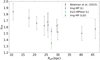 |
Fig. 10. Comparison between the total density slope, γtot, at the effective radius for CSWA 31 (colored squares) and the sample of group-scale lenses from Newman et al. (2015) (gray squares). The total density slopes inferred from our three reference models are shallower than the average values of other group-scale lenses. The discrepancy between lensing-only models and model Img-MP (L/D) is primarily caused by differences in the best-fit group halo component. |
We also compared the mass distribution in the extended dark-matter halo of CSWA 31 with the literature. Few strong-lensing groups have sets of multiple images covering beyond 100 kpc from the lens center, which results in less accurate lensing models. We thus rather compared with higher-mass (≳1014 M⊙) cluster-scale halos, using the high-precision lens models from Caminha et al. (2019). Since we cannot reliably estimate M200 and R200 without weak lensing, we rescaled the mass distribution of CSWA 31 to the cluster-scale lens RX J2129 with the closest θE. After rescaling, we obtained similar projected total mass profiles for both systems, suggesting that the self-similarity between high-mass dark-matter halos obtained by Caminha et al. (2019) extends to intermediate-mass, group-scale halos.
6.4. Constraints of the baryonic mass fraction
The baryonic and dark-matter mass fractions in CSWA 31 are distinguished in model Img-MP (L&D). In this section we discuss the robustness of this separation and characterize the combined dark-matter distribution. Figure 11 shows the cumulative projected mass profiles separately for each component in the BGG, indicating that dark matter strongly dominates the mass distribution up to rtr, BGG5.
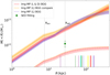 |
Fig. 11. Decomposition of dark-matter and baryonic mass components within the BGG from model Img-MP (L&D). We plot the cumulative profiles for the dark-matter (dashed red line) and baryonic (dot-dashed red line) components, and for the total mass of the BGG (solid red line). The purple curve shows the total mass profile of the BGG obtained in model Img-MP (L) using a single dPIE. The orange lines show the decomposition of dark-matter (dashed orange line) and baryonic (dot-dashed orange line) mass components within the BGG, from an additional lensing-only model with the same mass configuration as Img-MP (L&D). The shaded regions show the 1σ uncertainties on the mass distributions estimated from the 16th and 84th percentiles of the posterior PDFs. The baryonic mass profile from Img-MP (L&D) is lower than the stellar mass at Reff inferred independently from SED fitting (green square), and this discrepancy is driven by lensing constraints rather than JAM modeling. Vertical lines at the bottom indicate the positions of the multiple images used as lensing constraints. |
The total mass profile of the BGG from Img-MP (L&D) is consistent with the results obtained in Img-MP (L) from a single dPIE. The baryonic mass within the BGG remains well below 1012 M⊙ at all radii, and corresponds to an integrated stellar mass significantly lower than our independent estimate from SED fitting of (1.6 ± 0.4)×1012 M⊙. To compare the stellar masses obtained from these two independent methods at a common radius, we rescaled the result from SED fitting to the mass enclosed within Reff, using the baryonic mass profile from Img-MP (L&D) and assuming no radial gradient in the stellar mass-to-light ratio.
Modeling results from Img-MP (L&D) are used to infer the baryonic and dark-matter mass fractions in CSWA 31 from the joint contributions of the BGG, group-halo, and other perturbers. We define the baryon to total mass fraction within Reff as
 (36)
(36)
where Mbaryon is determined from the four best-fit PIEMDs in model Img-MP (L&D). We obtain  for CSWA 31 and compare in Fig. 12 with the average value for the Sloan Lens ACS (SLACS) sample of galaxy-scale lenses, and with group- and cluster-scale lenses compiled by Newman et al. (2015). In the comparison samples, fbaryon is defined as the baryon mass fraction of each lens systems, measured within the effective radius of the brightest central galaxy. fbaryon decreases progressively from galaxy- to cluster-scale lenses, while Reff increases for denser environments. The effective radius of the BGG in CSWA 31 falls near the median value of group-scale lenses, and near the lower envelope of cluster-scale lenses. However, fbaryon is much lower than the average value fbaryon = −0.78 for group-scale lenses analyzed in Newman et al. (2015). If we would assume our independent stellar mass estimate from SED fitting, we would obtain
  , placing CSWA 31 closer to group-scale lenses. For comparison, the joint lensing and stellar dynamical analysis of the Cosmic Horseshoe of Schuldt et al. (2019) leads to fbaryon in the range −0.40 to −0.52, close to the typical value of −0.60 for isolated early-type galaxies with masses ≳1012 M⊙ (e.g. Cappellari et al. 2013). The baryonic mass fraction in CSWA 31 is rather comparable to massive ellipticals with Reff ≃ 30 kpc in the center of large-scale halos.
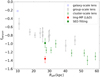 |
Fig. 12. Baryonic mass fraction within Reff for CSWA 31 compared to galaxy, group, and cluster scales in the literature (samples combined by Newman et al. 2015). The |

The difference between the stellar masses estimated from Img-MP (L&D) and from SED fitting might be driven by systematic errors in either of the two methods. Since the systematics in SED fitting have been extensively discussed in the literature (e.g., Conroy et al. 2013), we focus on quantifying the systematic uncertainties resulting from our novel modeling approach in Img-MP (L&D), testing our assumptions on lens mass profiles and on the dynamical modeling. First, we remodeled dark-matter within the BGG using a NFW profile instead of the SPEMD. This change degrades the fit mildly and further decreases fbaryon, suggesting that the mass parametrization does not contribute much to the systematic error budget of Img-MP (L&D). Second, the results from Img-MP (L&D) might also be affected by the assumptions involved in the theoretical dynamics modeling framework (see Sect. 5.2). We remodeled the separation between the baryonic and dark-matter components using the same mass configuration as Img-MP (L&D), but using only multiple image positions as constraints and discarding the BGG stellar kinematics. The cumulative mass profiles, the 1σ ranges, and the integrated stellar mass obtained from this new model are closely matching those from Img-MP (L&D), with only slightly larger error bars on the total mass profile (Fig. 11). This shows that the low fbaryon is driven by the lensing constraints rather than the JAM modeling. Consequently, while CSWA 31 is certainly dark-matter dominated toward the center, the actual baryonic mass fraction needs to be further studied to solve the discrepancy between these two independent methods.
7. Summary
In this work we have studied the inner structure of the group-scale lens CSWA 31 at z = 0.683 using HST near-infrared imaging and integral-field-unit spectroscopy from MUSE. Based on the spectroscopic confirmation of five sets of multiple images covering various projected separations from the lens center, we conducted a detailed analysis of the multi-scale mass distribution using various modeling approaches. First, we performed a lensing-only modeling, adopting a composite mass model to account for the central BGG, group members, and extended group-scale halo, and we compared the single- and multi-plane scenarios. We used image positions and extended arc morphologies as constraints. Secondly, we measured the spatially resolved stellar kinematics of the BGG to derive a joint lensing and dynamics model in order to improve the constraints toward the lens center and to attempt a separation between baryonic and dark-matter mass components in the BGG. For the dynamical modeling, we used the Jeans equations in cylindrical coordinates and assumed an axisymmetric underlying mass distribution. We compared the stellar mass of the BGG estimated independently from the joint lensing and dynamical analysis, and from SED fitting.
Despite small variations related to the different sets of input constraints, the relative contributions from the BGG and group-scale halo are remarkably consistent in our three reference models, demonstrating the self-consistency between strong lensing analyses based on image position and extended image modeling. We find that the ultra-massive BGG dominates the projected total mass profiles within 20 kpc, while the group-scale halo dominates at higher radii. The BGG represents 62.4% of the total mass enclosed within Rkin = 7.6 kpc, and the group-scale halo represents 72.3% of the total mass enclosed within RE, S0 = 70 kpc, the position of the brightest lensed arcs. Overall, CSWA 31 is a peculiar fossil group, strongly dark-matter dominated toward the central regions, and with a projected total mass profile similar to higher-mass cluster-scale halos. The total mass-density slope within the effective radius is shallower than isothermal, consistent with results obtained for lower-mass early-type galaxies in overdense environments ranging from galaxy groups to galaxy clusters.
In a future study we will put the properties of the central ultra-massive galaxy into context with the evolutionary trends of ellipticals in various environments to test predictions of galaxy evolution models. Furthermore, increasing the number of galaxy groups with such reliable mass decompositions will help constrain the processes driving galaxy evolution in group-scale environments. Multiband HST imaging with higher S/N and broader stellar kinematic maps from JWST/NIRSpec would significantly increase the accuracy of the baryon and dark-matter separations toward the central regions (the present map from MUSE probes only up to ≃25% of the BGG effective radius). Finally, the small asymmetries in the best-fit mass distribution of CSWA 31 highlight the limitations of JAM modeling, and further progress would benefit from more sophisticated dynamical modeling frameworks.
Other blue arcs were observed with VLT/X-shooter as part of programs 091.A-0852(A) (PI: Christensen) and 094.A-0684(A) (PI: Grillo) but did not provide secure identifications of additional multiple image families.
The total mass also accounts for group members such that the sum of BGG and group-halo only is lower than the total mass.
We obtain the same results by excluding set S4 that has a counter-image at ∼20 kpc from the BGG center.
We determine the γtot for the total mass of BGG and group halo. We exclude the group members from the total mass in the Sect. 6.3 to simplify the calculation because the mass of the group members are negligible given the results from Sect. 6.2 and most of them are located outside of the region enclosed by the effective radius of the BGG as shown in HST imaging.
Note that Fig. 11 shows the decomposition of the BGG into dark-matter and baryonic component, while Fig. 9 shows the decomposition of the whole system CSWA 31 into BGG and group halo. Both figures show the total mass of the BGG, albeit with different line styles: in Fig. 11 with solid lines and in Fig. 9 with dot-dashed lines.
Acknowledgments
We would like to thank the anonymous referee whose comments were helpful in improving the paper. We thank A. Halkola for software support on GLEE and GLaD. G. B. Caminha, S. H. Suyu, A. Yıldırım, G. Chirivì and S. Schuldt acknowledge the Max Planck Society for support through the Max Planck Research Group for S. H. Suyu. G.B.C. also thanks the academic support from the German Centre for Cosmological Lensing. This research is supported in part by the Excellence Cluster ORIGINS which is funded by the Deutsche Forschungsgemeinschaft (DFG, German Research Foundation) under Germany’s Excellence Strategy – EXC-2094 – 390783311. This research is based on observations made with the NASA/ESA Hubble Space Telescope obtained from the Space Telescope Science Institute, which is operated by the Association of Universities for Research in Astronomy, Inc., under NASA contract NAS 5-26555. These observations are associated with program GO-15253. This work is also based on observations collected at the European Organisation for Astronomical Research in the Southern Hemisphere under ESO program 0104.A-0830(A).
References
- Auger, M. W., Fassnacht, C. D., Wong, K. C., et al. 2008, ApJ, 673, 778 [NASA ADS] [CrossRef] [Google Scholar]
- Auger, M. W., Treu, T., Bolton, A. S., et al. 2009, ApJ, 705, 1099 [Google Scholar]
- Bacon, R., Vernet, J., Borisova, E., et al. 2014, The Messenger, 157, 13 [NASA ADS] [Google Scholar]
- Barkana, R. 1998, ApJ, 502, 531 [NASA ADS] [CrossRef] [Google Scholar]
- Barnabè, M., Czoske, O., Koopmans, L. V. E., et al. 2009, MNRAS, 399, 21 [CrossRef] [Google Scholar]
- Barnabè, M., Dutton, A. A., Marshall, P. J., et al. 2012, MNRAS, 423, 1073 [Google Scholar]
- Bayliss, M. B., Johnson, T., Gladders, M. D., Sharon, K., & Oguri, M. 2014, ApJ, 783, 41 [NASA ADS] [CrossRef] [Google Scholar]
- Belokurov, V., Evans, N. W., Hewett, P. C., et al. 2009, MNRAS, 392, 104 [NASA ADS] [CrossRef] [Google Scholar]
- Bernardi, M., Roche, N., Shankar, F., & Sheth, R. K. 2011, MNRAS, 412, L6 [NASA ADS] [CrossRef] [Google Scholar]
- Bertin, E. 2006, in Astronomical Data Analysis Software and Systems XV, eds. C. Gabriel, C. Arviset, D. Ponz, & S. Enrique, ASP Conf. Ser., 351, 112 [Google Scholar]
- Bertin, E. 2010, Astrophysics Source Code Library [record ascl:1010.068] [Google Scholar]
- Bertin, E., & Arnouts, S. 1996, A&AS, 117, 393 [NASA ADS] [CrossRef] [EDP Sciences] [Google Scholar]
- Binney, J., & Tremaine, S. 1987, Galactic Dynamics (Princeton: Princeton University Press) [Google Scholar]
- Birrer, S., & Treu, T. 2021, A&A, 649, A61 [NASA ADS] [CrossRef] [EDP Sciences] [Google Scholar]
- Blandford, R., & Narayan, R. 1986, ApJ, 310, 568 [Google Scholar]
- Blumenthal, G. R., Faber, S. M., Flores, R., & Primack, J. R. 1986, ApJ, 301, 27 [Google Scholar]
- Bolton, A. S., Brownstein, J. R., Kochanek, C. S., et al. 2012, ApJ, 757, 82 [NASA ADS] [CrossRef] [Google Scholar]
- Boquien, M., Burgarella, D., Roehlly, Y., et al. 2019, A&A, 622, A103 [NASA ADS] [CrossRef] [EDP Sciences] [Google Scholar]
- Brewer, B. J., Lewis, G. F., Belokurov, V., et al. 2011, MNRAS, 412, 2521 [NASA ADS] [CrossRef] [Google Scholar]
- Bruzual, G., & Charlot, S. 2003, MNRAS, 344, 1000 [NASA ADS] [CrossRef] [Google Scholar]
- Burgarella, D., Buat, V., & Iglesias-Páramo, J. 2005, MNRAS, 360, 1413 [NASA ADS] [CrossRef] [Google Scholar]
- Caminha, G. B., Grillo, C., Rosati, P., et al. 2017, A&A, 600, A90 [NASA ADS] [CrossRef] [EDP Sciences] [Google Scholar]
- Caminha, G. B., Rosati, P., Grillo, C., et al. 2019, A&A, 632, A36 [NASA ADS] [CrossRef] [EDP Sciences] [Google Scholar]
- Cappellari, M. 2008, MNRAS, 390, 71 [NASA ADS] [CrossRef] [Google Scholar]
- Cappellari, M., & Copin, Y. 2003, MNRAS, 342, 345 [Google Scholar]
- Cappellari, M., & Emsellem, E. 2004, PASP, 116, 138 [Google Scholar]
- Cappellari, M., Emsellem, E., Bacon, R., et al. 2007, MNRAS, 379, 418 [Google Scholar]
- Cappellari, M., McDermid, R. M., Alatalo, K., et al. 2013, MNRAS, 432, 1862 [NASA ADS] [CrossRef] [Google Scholar]
- Cappellari, M., Romanowsky, A. J., Brodie, J. P., et al. 2015, ApJ, 804, L21 [NASA ADS] [CrossRef] [Google Scholar]
- Charlot, S., & Fall, S. M. 2000, ApJ, 539, 718 [Google Scholar]
- Chen, G. C. F., Fassnacht, C. D., Suyu, S. H., et al. 2021, A&A, 652, A7 [NASA ADS] [CrossRef] [EDP Sciences] [Google Scholar]
- Chirivì, G., Suyu, S. H., Grillo, C., et al. 2018, A&A, 614, A8 [NASA ADS] [CrossRef] [EDP Sciences] [Google Scholar]
- Chirivì, G., Yıldırım, A., Suyu, S. H., & Halkola, A. 2020, A&A, 643, A135 [EDP Sciences] [Google Scholar]
- Conroy, C., Dutton, A. A., Graves, G. J., Mendel, J. T., & van Dokkum, P. G. 2013, ApJ, 776, L26 [NASA ADS] [CrossRef] [Google Scholar]
- Croton, D. J., Springel, V., White, S. D. M., et al. 2006, MNRAS, 365, 11 [Google Scholar]
- D’Aloisio, A., Natarajan, P., & Shapiro, P. R. 2014, MNRAS, 445, 3581 [CrossRef] [Google Scholar]
- Deason, A. J., Auger, M. W., Belokurov, V., & Evans, N. W. 2013, ApJ, 773, 7 [NASA ADS] [CrossRef] [Google Scholar]
- Derkenne, C., McDermid, R. M., Poci, A., et al. 2021, MNRAS, 506, 3691 [NASA ADS] [CrossRef] [Google Scholar]
- Dutton, A. A., & Treu, T. 2014, MNRAS, 438, 3594 [NASA ADS] [CrossRef] [Google Scholar]
- Dutton, A. A., Brewer, B. J., Marshall, P. J., et al. 2011, MNRAS, 417, 1621 [NASA ADS] [CrossRef] [Google Scholar]
- Eke, V. R., Baugh, C. M., Cole, S., et al. 2004, MNRAS, 348, 866 [NASA ADS] [CrossRef] [Google Scholar]
- Elíasdóttir, Á., Limousin, M., Richard, J., et al. 2007, ArXiv e-prints [arXiv:0710.5636] [Google Scholar]
- Emsellem, E., Cappellari, M., Krajnović, D., et al. 2007, MNRAS, 379, 401 [Google Scholar]
- Falco, E. E., Gorenstein, M. V., & Shapiro, I. I. 1985, ApJ, 289, L1 [Google Scholar]
- Fassbender, R., Böhringer, H., Nastasi, A., et al. 2011, New J. Phys., 13, 125014 [Google Scholar]
- Foreman-Mackey, D., Hogg, D. W., Lang, D., & Goodman, J. 2013, PASP, 125, 306 [Google Scholar]
- Fruchter, A. S., et al. 2010, 2010 Space Telescope Science Institute Calibration Workshop, 382 [Google Scholar]
- Gallazzi, A., Bell, E. F., Zibetti, S., Brinchmann, J., & Kelson, D. D. 2014, ApJ, 788, 72 [Google Scholar]
- Gavazzi, R., Treu, T., Rhodes, J. D., et al. 2007, ApJ, 667, 176 [Google Scholar]
- Gavazzi, R., Treu, T., Koopmans, L. V. E., et al. 2008, ApJ, 677, 1046 [NASA ADS] [CrossRef] [Google Scholar]
- Grillo, C., Christensen, L., Gallazzi, A., & Rasmussen, J. 2013, MNRAS, 433, 2604 [NASA ADS] [CrossRef] [Google Scholar]
- Grillo, C., Suyu, S. H., Rosati, P., et al. 2015, ApJ, 800, 38 [Google Scholar]
- Grillo, C., Karman, W., Suyu, S. H., et al. 2016, ApJ, 822, 78 [Google Scholar]
- Jauzac, M., Mahler, G., Edge, A. C., et al. 2019, MNRAS, 483, 3082 [Google Scholar]
- Johnson, L. E., Irwin, J. A., White, R. E., III, et al. 2018, ApJ, 856, 131 [NASA ADS] [CrossRef] [Google Scholar]
- Jones, L. R., Ponman, T. J., Horton, A., et al. 2003, MNRAS, 343, 627 [NASA ADS] [CrossRef] [Google Scholar]
- Khosroshahi, H. G., Ponman, T. J., & Jones, L. R. 2007, MNRAS, 377, 595 [NASA ADS] [CrossRef] [Google Scholar]
- Koopmans, L. V. E., & Treu, T. 2003, ApJ, 583, 606 [NASA ADS] [CrossRef] [Google Scholar]
- Koopmans, L. V. E., Treu, T., Bolton, A. S., Burles, S., & Moustakas, L. A. 2006, ApJ, 649, 599 [Google Scholar]
- Lagattuta, D. J., Richard, J., Clément, B., et al. 2017, MNRAS, 469, 3946 [Google Scholar]
- Leethochawalit, N., Jones, T. A., Ellis, R. S., et al. 2016, ApJ, 820, 84 [NASA ADS] [CrossRef] [Google Scholar]
- Li, R., Shu, Y., & Wang, J. 2018, MNRAS, 480, 431 [NASA ADS] [CrossRef] [Google Scholar]
- Limousin, M., Sommer-Larsen, J., Natarajan, P., & Milvang-Jensen, B. 2009a, ApJ, 696, 1771 [NASA ADS] [CrossRef] [Google Scholar]
- Limousin, M., Cabanac, R., Gavazzi, R., et al. 2009b, A&A, 502, 445 [NASA ADS] [CrossRef] [EDP Sciences] [Google Scholar]
- Limousin, M., Richard, J., Jullo, E., et al. 2016, A&A, 588, A99 [NASA ADS] [CrossRef] [EDP Sciences] [Google Scholar]
- Loeb, A., & Peebles, P. J. E. 2003, ApJ, 589, 29 [NASA ADS] [CrossRef] [Google Scholar]
- Mahler, G., Richard, J., Clément, B., et al. 2018, MNRAS, 473, 663 [Google Scholar]
- Mahler, G., Sharon, K., Fox, C., et al. 2019, ApJ, 873, 96 [Google Scholar]
- Maller, A. H., Simard, L., Guhathakurta, P., et al. 2000, ApJ, 533, 194 [NASA ADS] [CrossRef] [Google Scholar]
- Martizzi, D., Teyssier, R., Moore, B., & Wentz, T. 2012, MNRAS, 422, 3081 [NASA ADS] [CrossRef] [Google Scholar]
- More, A., Cabanac, R., More, S., et al. 2012, ApJ, 749, 38 [NASA ADS] [CrossRef] [Google Scholar]
- Moster, B. P., Naab, T., & White, S. D. M. 2020, MNRAS, 499, 4748 [Google Scholar]
- Muñoz, R. P., Motta, V., Verdugo, T., et al. 2013, A&A, 552, A80 [NASA ADS] [CrossRef] [EDP Sciences] [Google Scholar]
- Munari, E., Biviano, A., Borgani, S., Murante, G., & Fabjan, D. 2013, MNRAS, 430, 2638 [Google Scholar]
- Naab, T., Johansson, P. H., Ostriker, J. P., & Efstathiou, G. 2007, ApJ, 658, 710 [NASA ADS] [CrossRef] [Google Scholar]
- Naab, T., Johansson, P. H., & Ostriker, J. P. 2009, ApJ, 699, L178 [Google Scholar]
- Navarro, J. F., Frenk, C. S., & White, S. D. M. 1996, ApJ, 462, 563 [Google Scholar]
- Navarro, J. F., Frenk, C. S., & White, S. D. M. 1997, ApJ, 490, 493 [Google Scholar]
- Newman, A. B., Treu, T., Ellis, R. S., & Sand, D. J. 2013a, ApJ, 765, 25 [NASA ADS] [CrossRef] [Google Scholar]
- Newman, A. B., Treu, T., Ellis, R. S., et al. 2013b, ApJ, 765, 24 [NASA ADS] [CrossRef] [Google Scholar]
- Newman, A. B., Ellis, R. S., & Treu, T. 2015, ApJ, 814, 26 [NASA ADS] [CrossRef] [Google Scholar]
- Nipoti, C., Treu, T., Ciotti, L., & Stiavelli, M. 2004, MNRAS, 355, 1119 [NASA ADS] [CrossRef] [Google Scholar]
- Noll, S., Burgarella, D., Giovannoli, E., et al. 2009, A&A, 507, 1793 [NASA ADS] [CrossRef] [EDP Sciences] [Google Scholar]
- Pacifici, C., Kassin, S. A., Weiner, B. J., et al. 2016, ApJ, 832, 79 [Google Scholar]
- Pontzen, A., & Governato, F. 2012, MNRAS, 421, 3464 [NASA ADS] [CrossRef] [Google Scholar]
- Remus, R.-S., Burkert, A., Dolag, K., et al. 2013, ApJ, 766, 71 [NASA ADS] [CrossRef] [Google Scholar]
- Rescigno, U., Grillo, C., Lombardi, M., et al. 2020, A&A, 635, A98 [EDP Sciences] [Google Scholar]
- Richard, J., Smith, G. P., Kneib, J.-P., et al. 2010, MNRAS, 404, 325 [NASA ADS] [Google Scholar]
- Richard, J., Claeyssens, A., Lagattuta, D., et al. 2021, A&A, 646, A83 [EDP Sciences] [Google Scholar]
- Salpeter, E. E. 1955, ApJ, 121, 161 [Google Scholar]
- Sand, D. J., Treu, T., Ellis, R. S., Smith, G. P., & Kneib, J.-P. 2008, ApJ, 674, 711 [NASA ADS] [CrossRef] [Google Scholar]
- Schaller, M., Frenk, C. S., Bower, R. G., et al. 2015, MNRAS, 452, 343 [NASA ADS] [CrossRef] [Google Scholar]
- Schneider, P. 2006, in Saas-Fee Advanced Course 33: Gravitational Lensing: Strong, Weak and Micro, eds. G. Meylan, P. Jetzer, P. North, et al., 1 [Google Scholar]
- Schuldt, S., Chirivì, G., Suyu, S. H., et al. 2019, A&A, 631, A40 [NASA ADS] [CrossRef] [EDP Sciences] [Google Scholar]
- Sérsic, J. L. 1963, Boletin de la Asociacion Argentina de Astronomia La Plata Argentina, 6, 41 [Google Scholar]
- Shajib, A. J., Treu, T., Birrer, S., & Sonnenfeld, A. 2021, MNRAS, 503, 2380 [Google Scholar]
- Sommer-Larsen, J. 2006, MNRAS, 369, 958 [Google Scholar]
- Sonnenfeld, A., Treu, T., Gavazzi, R., et al. 2013, ApJ, 777, 98 [Google Scholar]
- Sonnenfeld, A., Treu, T., Marshall, P. J., et al. 2015, ApJ, 800, 94 [Google Scholar]
- Sonnenfeld, A., Leauthaud, A., Auger, M. W., et al. 2018, MNRAS, 481, 164 [Google Scholar]
- Soto, K. T., Lilly, S. J., Bacon, R., Richard, J., & Conseil, S. 2016, MNRAS, 458, 3210 [Google Scholar]
- Spiniello, C., Koopmans, L. V. E., Trager, S. C., Czoske, O., & Treu, T. 2011, MNRAS, 417, 3000 [NASA ADS] [CrossRef] [Google Scholar]
- Springel, V., Di Matteo, T., & Hernquist, L. 2005, MNRAS, 361, 776 [Google Scholar]
- Stark, D. P., Auger, M., Belokurov, V., et al. 2013, MNRAS, 436, 1040 [Google Scholar]
- Subramanian, K., Cen, R., & Ostriker, J. P. 2000, ApJ, 538, 528 [NASA ADS] [CrossRef] [Google Scholar]
- Suyu, S. H., & Halkola, A. 2010, A&A, 524, A94 [NASA ADS] [CrossRef] [EDP Sciences] [Google Scholar]
- Suyu, S. H., Marshall, P. J., Hobson, M. P., & Blandford, R. D. 2006, MNRAS, 371, 983 [Google Scholar]
- Suyu, S. H., Hensel, S. W., McKean, J. P., et al. 2012, ApJ, 750, 10 [Google Scholar]
- Suyu, S. H., Treu, T., Hilbert, S., et al. 2014, ApJ, 788, L35 [NASA ADS] [CrossRef] [Google Scholar]
- Tacchella, S., Conroy, C., Faber, S. M., et al. 2022, ApJ, 926, 134 [NASA ADS] [CrossRef] [Google Scholar]
- Thomas, D., Maraston, C., Bender, R., & Mendes de Oliveira, C. 2005, ApJ, 621, 673 [Google Scholar]
- Tortora, C., La Barbera, F., Napolitano, N. R., et al. 2014, MNRAS, 445, 115 [NASA ADS] [CrossRef] [Google Scholar]
- Treu, T., & Koopmans, L. V. E. 2004, ApJ, 611, 739 [Google Scholar]
- Valdes, F., Gupta, R., Rose, J. A., Singh, H. P., & Bell, D. J. 2004, ApJS, 152, 251 [Google Scholar]
- van de Ven, G., Falcón-Barroso, J., McDermid, R. M., et al. 2010, ApJ, 719, 1481 [Google Scholar]
- van der Wel, A., Franx, M., van Dokkum, P. G., et al. 2014, ApJ, 788, 28 [Google Scholar]
- Veale, M., Ma, C.-P., Greene, J. E., et al. 2018, MNRAS, 473, 5446 [Google Scholar]
- Vegetti, S., Lagattuta, D. J., McKean, J. P., et al. 2012, Nature, 481, 341 [NASA ADS] [CrossRef] [Google Scholar]
- Verhamme, A., Garel, T., Ventou, E., et al. 2018, MNRAS, 478, L60 [Google Scholar]
- Wang, Y., Vogelsberger, M., Xu, D., et al. 2019, MNRAS, 490, 5722 [NASA ADS] [CrossRef] [Google Scholar]
- Wang, Y., Mao, S., Vogelsberger, M., et al. 2022, MNRAS, 513, 6134 [NASA ADS] [CrossRef] [Google Scholar]
- Weilbacher, P. M., Streicher, O., Urrutia, T., et al. 2014, in Astronomical Data Analysis Software and Systems XXIII, eds. N. Manset, & P. Forshay, ASP Conf. Ser., 485, 451 [Google Scholar]
- Yıldırım, A., Suyu, S. H., & Halkola, A. 2020, MNRAS, 493, 4783 [Google Scholar]
- Yıldırım, A., Suyu, S. H., Chen, G. C. F., & Komatsu, E. 2021, ArXiv e-prints [arXiv:2109.14615] [Google Scholar]
Appendix A: Light profiles and spectral energy distribution
The Chameleon profile used to model the BGG light distribution in Sect. 5 consists of two isothermal profiles with different core radii that mimic a Sérsic profile. It is defined in Cartesian coordinates (x, y) as
 (A.1)
(A.1)
where q is the axis ratio, ωt and ωc are the different core radii, I0 is the amplitude. To keep the I(x, y) > 0 we imposed ωt > ωc. The Chameleon profile can be rotated by the position angle θPA. It can be directly linked to isothermal mass profiles using a mass-to-light ratio.
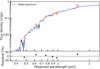 |
Fig. A.1. SED of the BGG in CSWA 31. The observed Pan-STARRS (red circles) and HST (red square) fluxes are plotted, with uncertainties smaller than the symbols, together with the best-fit SED obtained with CIGALE (blue curve) and the corresponding model fluxes (orange markers). The bottom panel shows the relative residuals of the fit. |
Appendix B: MUSE redshift catalog and spectra of multiple images
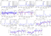 |
Fig. B.1. MUSE 1D spectra of the multiple images in sets S2, S3, S4, and S5, which are newly confirmed. The blue lines are the observed spectra in units of 10−20 erg s−1 cm−2 Å−1. They are extracted using circular apertures of 0.8″ radii, except for the faint images S5(a) and S5(b), which are jointly extracted along the extended arc. The gray regions indicate the data variance. The vertical lines mark the main spectral features used to measure redshifts, and the red curves show the best-fit templates used to estimate the redshifts of images in sets S3 and S5. The best-fit systemic redshift reported for set S4 comes from the [CIII] emission line detected in image S4(b). Lyα lines are detected in all three images of S4 and are slightly redshifted (see also, e.g., Verhamme et al. 2018). |
Spectroscopic redshift catalog from MUSE.
Appendix C: Image position models in the single- and multi-plane scenarios
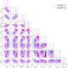 |
Fig. C.1. Joint posterior PDFs for lensing-only models Img-SP (L) and Img-MP (L) based on the centroid positions of multiple images. The three shaded areas show the 68.3%, 95.4% and, 99.7% credible regions. The 1D histograms show the marginalized PDFs of each mass parameter, and vertical lines highlight the 1σ ranges. |
Appendix D: Extended image modeling of source S3
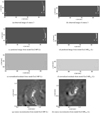 |
Fig. D.1. Surface brightness reconstruction for lensed source S3 at redshift z = 3.4280 from two different extended image models. We show the nearby group members included in the light modeling, while other objects within the gray regions are masked out. From top to bottom: Observed HST F160W images, the best-fit models, the normalized residuals in the range −9.5σ to 5σ, and the reconstructed source-plane morphology. Left column: Reconstruction from model Esr2-MP (L), which shows excellent residuals for the rightmost arc but significant overfitting of the light emission from the compact counterimage on the left. Right column: Same but for model Esr2-MPtest (L) based on a new mask that excludes the upper faint, diffuse region of the arc. This model improves the fit of the counterimage of S3. |
Appendix E: Critical curves of three reference lens models
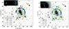 |
Fig. E.1. Critical curves of three reference lens models. Left: Critical curves for models Img-MP (L) (solid purple line), Esr2-MPtest (L) (solid cyan line), and Img-MP (L/D) (solid green line), and for the redshift of S0. The upper-left inset zooms in on a 5″ × 3″ rectangle to show more details of critical curves in the central region. Right: Same critical curves but for the redshift of S3. The upper-left inset zooms in on an 8″ × 5″ rectangle around the central region where the third image of S3 falls (blue “cross”). No critical curves pass through S3(b), the extended arc of S3, indicating that it comprises a single distorted image. |
All Tables
Position, spectroscopic redshift, and (F438W − F160W) color for the BGG and multiple images used in the modeling.
Best-fit and marginalized values with 1σ uncertainties for the near-infrared light modeling of the BGG in CSWA 31.
Best-fit and marginalized values with 1σ uncertainties for the parameters of our lensing-only models based on image positions, in the single-plane (Img-SP (L)) and multi-plane scenarios (Img-MP (L)).
Best-fit and marginalized values with 1σ uncertainties for the parameters of our lensing-only models based on the extended surface brightness distribution of sources S0 and S3 and on the positions of multiple images from other sets.
Best-fit and marginalized values with 1σ uncertainties for model Img-MP (L/D) based on joint constraints from strong lensing and stellar dynamics.
All Figures
|
Fig. 1. HST/WFC3 image of CSWA 31 and its surrounding environment in the F160W band. The orientation is marked by the black arrows in the bottom-right of the figure, and the ruler indicates a physical scale of 150 kpc in the main lens plane at z = 0.683. The large black box marks the total 1′ × 1′ coverage of MUSE observations. The small 8″ × 8″ black box in the center shows the field of view considered for the dynamical analysis of the main lens galaxy, and the x′ and y′ arrows show the orientation adopted for the kinematic maps (see Sect. 5). The sets of spectroscopically confirmed multiple images used in our analysis are marked with circles, with a different color for each set. The image sets S0 and S1 are bright knots from the same spiral galaxy at z = 1.4869, with a zoomed-in image of S0(d) in the left inset. The right inset shows the bright arc from source galaxy S3 at z = 2.763. The multiple images of source 4 (S4) are identified with MUSE and undetected in this HST image. |
| In the text | |
|
Fig. 2. HST F160W image showing the BGG (red star), group members (orange stars), the reference galaxy used in the scaling relations (purple star), and sets of multiple images (circles). We modeled the emission of group members 1, 2, 3, 4, and 5 (cyan filled stars) together with the BGG in order to minimize light contamination on the nearby lensed arcs. Given the significant contribution of group members 1, 2, 6, and 7 to the light deflection angles, their Einstein radius were optimized separately. The image positions predicted by models Img-SP (L) and Img-MP (L) are marked by plus and cross symbols, respectively. Similarly, the mean weighted source positions reconstructed by models Img-SP (L) and Img-MP (L) are indicated with bold plus and cross symbols, respectively. The solid purple line shows the critical curve of model Img-SP (L) with regards to S0. The upper-left inset zooms in on the 3.6″ × 4.9″ rectangle to highlight the intrinsic positions of S0, S1, and S5 in both models. The solid purple line shows the critical curve of model Img-MP(L) for z = 1.487, the redshift of S0. The critical curves of other reference models are shown in Appendix E. |
| In the text | |
|
Fig. 3. Best-fit model for the light distribution of the BGG and five nearby group members. From top to bottom: observed HST F160W band image, the best-fit model, and the normalized residuals in the range −7σ to 7σ. In all three images, the constant areas are the masks covering the lensed arcs and other objects in the field. The panels cover a field of view of 36″ × 22″ and are oriented in the same way as in Fig. 1, with north approximately toward the bottom. |
| In the text | |
|
Fig. 4. Surface brightness reconstruction of source S0 at redshift z = 1.4869 from the best-fit model Esr2-MPtest (L). Two nearby group members are included in the modeling, while other objects within the gray regions are masked out. We show the observed HST F160W image over a field of view of 36″ × 22″ (top left), the best-fit model of the main arc, BGG and group members (top right), the normalized residual (bottom left) in the range −7σ to 7σ, and the source-plane reconstruction of S0 over a field of 2.1″ × 2.1″ (bottom right). The arc is well fitted and does not show significant residuals in the image plane. S0 has a clear spiral shape in the source plane. It is well reconstructed in all our lens models, with an intrinsic morphology consistent with our reference model Esr2-MPtest (L). |
| In the text | |
|
Fig. 5. Spatially resolved stellar kinematics of the BGG in 11 Voronoi bins with sufficient S/N extracted over a 8″ × 8″ field of view. The maps show the line-of-sight velocities v (left), the projected velocity dispersions, σ (middle), and the second velocity moments, Vrms (right). The orientation of the figure differs from the previous figures. The x′ axis points to the north and is aligned with the major axis of the BGG, while the y′ axis points to the west. Note that the spectrum shown in Fig. 6 corresponds to the central resolution element. |
| In the text | |
|
Fig. 6. Example of spectral fitting with pPXF for one resolution element in our binned data cube (the central bin in Fig. 5). The black and red lines show the observed spectrum normalized to unity and the best-fit stellar template, respectively. The green symbols at the bottom are the fit residuals, and the blue lines with gray-shaded regions show positions of gas emission lines masked during the fit. The most prominent spectral features used for the fit are the Ca H and K lines at 3935 Å and 3970 Å in the rest frame, the continuum break at 4000 Å, the G-band feature at 4305 Å, and the Hβ line at 4863 Å. Such high-S/N spectra are used to extract robust stellar kinematics for the BGG out to ≃0.5 Reff (see Fig. 5). |
| In the text | |
|
Fig. 7. Modeled stellar kinematics of the BGG. Left: Vrms radial profile predicted by the joint lensing and dynamical modeling Img-MP (L/D) (green triangles) from the most-probable model compared to the Vrms measured over the 11 Voronoi bins and their 1σ uncertainties (gray points). The radial position of each resolution element is defined with respect to the BGG centroid. The observed Vrms are consistent with a flat profile, and predicted values are within the 1σ ranges in most bins. Right: predicted Vrms map from model Img-MP (L/D), showing that this model does not fully recover the angular structure of Vrms in Fig. 5. |
| In the text | |
|
Fig. 8. Joint posterior PDFs for our three reference models, corresponding to the lensing-only models based on image positions (Img-MP (L), purple contours) and on extended surface brightness distributions (Esr2-MPtest (L), cyan contours), and to the joint modeling with strong lensing and dynamics (Img-MP (L/D), green contours). We focus on the most important mass parameters that describe the BGG and the extended group-scale halo. The three shaded areas on the joint PDFs show the 68.3%, 95.4%, and 99.7% credible regions. The 1D histograms show the marginalized PDFs for the selected mass parameters, and the vertical lines mark the 1σ confidence intervals. The model based on extended image fitting has narrower contours due to the large number of constraints from the lensed source morphologies. |
| In the text | |
|
Fig. 9. Cumulative mass profiles as a function of radial separation from the BGG center, for the BGG (dot-dashed lines), group-scale (dashed lines), and total (solid lines) mass components of CSWA 31. The shaded regions show the 1σ uncertainties on the mass distributions estimated from the 16th and 84th percentiles of the posterior PDFs. The reference models Img-MP (L), Esr2-MPtest (L), and Img-MP (L/D) are compared using the same colors as in Fig. 8. Vertical lines in the bottom indicate the positions of multiple images used as constraints. The solid pink line with shaded regions shows the total mass of CSWA 31 with 1σ uncertainties estimated by G13, using only image positions of set S0 (green vertical lines) as constraints. The gray line at Rkin = 7.6 kpc shows the coverage of the MUSE spatially resolved stellar kinematics. We also mark Reff to ease comparison with other lenses in the literature. |
| In the text | |
|
Fig. 10. Comparison between the total density slope, γtot, at the effective radius for CSWA 31 (colored squares) and the sample of group-scale lenses from Newman et al. (2015) (gray squares). The total density slopes inferred from our three reference models are shallower than the average values of other group-scale lenses. The discrepancy between lensing-only models and model Img-MP (L/D) is primarily caused by differences in the best-fit group halo component. |
| In the text | |
|
Fig. 11. Decomposition of dark-matter and baryonic mass components within the BGG from model Img-MP (L&D). We plot the cumulative profiles for the dark-matter (dashed red line) and baryonic (dot-dashed red line) components, and for the total mass of the BGG (solid red line). The purple curve shows the total mass profile of the BGG obtained in model Img-MP (L) using a single dPIE. The orange lines show the decomposition of dark-matter (dashed orange line) and baryonic (dot-dashed orange line) mass components within the BGG, from an additional lensing-only model with the same mass configuration as Img-MP (L&D). The shaded regions show the 1σ uncertainties on the mass distributions estimated from the 16th and 84th percentiles of the posterior PDFs. The baryonic mass profile from Img-MP (L&D) is lower than the stellar mass at Reff inferred independently from SED fitting (green square), and this discrepancy is driven by lensing constraints rather than JAM modeling. Vertical lines at the bottom indicate the positions of the multiple images used as lensing constraints. |
| In the text | |
|
Fig. 12. Baryonic mass fraction within Reff for CSWA 31 compared to galaxy, group, and cluster scales in the literature (samples combined by Newman et al. 2015). The |
| In the text | |
|
Fig. A.1. SED of the BGG in CSWA 31. The observed Pan-STARRS (red circles) and HST (red square) fluxes are plotted, with uncertainties smaller than the symbols, together with the best-fit SED obtained with CIGALE (blue curve) and the corresponding model fluxes (orange markers). The bottom panel shows the relative residuals of the fit. |
| In the text | |
|
Fig. B.1. MUSE 1D spectra of the multiple images in sets S2, S3, S4, and S5, which are newly confirmed. The blue lines are the observed spectra in units of 10−20 erg s−1 cm−2 Å−1. They are extracted using circular apertures of 0.8″ radii, except for the faint images S5(a) and S5(b), which are jointly extracted along the extended arc. The gray regions indicate the data variance. The vertical lines mark the main spectral features used to measure redshifts, and the red curves show the best-fit templates used to estimate the redshifts of images in sets S3 and S5. The best-fit systemic redshift reported for set S4 comes from the [CIII] emission line detected in image S4(b). Lyα lines are detected in all three images of S4 and are slightly redshifted (see also, e.g., Verhamme et al. 2018). |
| In the text | |
|
Fig. C.1. Joint posterior PDFs for lensing-only models Img-SP (L) and Img-MP (L) based on the centroid positions of multiple images. The three shaded areas show the 68.3%, 95.4% and, 99.7% credible regions. The 1D histograms show the marginalized PDFs of each mass parameter, and vertical lines highlight the 1σ ranges. |
| In the text | |
|
Fig. D.1. Surface brightness reconstruction for lensed source S3 at redshift z = 3.4280 from two different extended image models. We show the nearby group members included in the light modeling, while other objects within the gray regions are masked out. From top to bottom: Observed HST F160W images, the best-fit models, the normalized residuals in the range −9.5σ to 5σ, and the reconstructed source-plane morphology. Left column: Reconstruction from model Esr2-MP (L), which shows excellent residuals for the rightmost arc but significant overfitting of the light emission from the compact counterimage on the left. Right column: Same but for model Esr2-MPtest (L) based on a new mask that excludes the upper faint, diffuse region of the arc. This model improves the fit of the counterimage of S3. |
| In the text | |
|
Fig. E.1. Critical curves of three reference lens models. Left: Critical curves for models Img-MP (L) (solid purple line), Esr2-MPtest (L) (solid cyan line), and Img-MP (L/D) (solid green line), and for the redshift of S0. The upper-left inset zooms in on a 5″ × 3″ rectangle to show more details of critical curves in the central region. Right: Same critical curves but for the redshift of S3. The upper-left inset zooms in on an 8″ × 5″ rectangle around the central region where the third image of S3 falls (blue “cross”). No critical curves pass through S3(b), the extended arc of S3, indicating that it comprises a single distorted image. |
| In the text | |
Current usage metrics show cumulative count of Article Views (full-text article views including HTML views, PDF and ePub downloads, according to the available data) and Abstracts Views on Vision4Press platform.
Data correspond to usage on the plateform after 2015. The current usage metrics is available 48-96 hours after online publication and is updated daily on week days.
Initial download of the metrics may take a while.