| Issue |
A&A
Volume 666, October 2022
|
|
|---|---|---|
| Article Number | A102 | |
| Number of page(s) | 22 | |
| Section | Extragalactic astronomy | |
| DOI | https://doi.org/10.1051/0004-6361/202142831 | |
| Published online | 12 October 2022 | |
The chemical footprint of AGN feedback in the outflowing circumnuclear disk of NGC 1068
1
Leiden Observatory, Leiden University, PO Box 9513 2300 RA Leiden, The Netherlands
e-mail: This email address is being protected from spambots. You need JavaScript enabled to view it.
2
Department of Physics and Astronomy, University College London, Gower Street, London WC1E 6BT, UK
3
Observatorio Astronómico Nacional (OAN-IGN)-Observatorio de Madrid, Alfonso XII, 3, 28014 Madrid, Spain
4
Institute of Astronomy, Graduate School of Science, The University of Tokyo, Osawa, Mitaka, Tokyo 181-0015, Japan
5
Division of Particle and Astrophysical Science, Graduate School of Science, Nagoya University, Furocho, Chikusa-ku, Nagoya, Aichi 464-8602, Japan
6
European Southern Observatory, Alonso de Córdova, 3107, Vitacura, Santiago 763-0355, Chile
7
Joint ALMA Observatory, Alonso de Córdova, 3107, Vitacura, Santiago 763-0355, Chile
8
Max-Planck-Institut für Radioastronomie, Auf dem Hügel 69, 53121 Bonn, Germany
9
Centro de Astrobiología (CSIC/INTA), Ctra de Torrejón a Ajalvir, km 4, 28850 Torrejón de Ardoz, Madrid, Spain
Received:
3
December
2021
Accepted:
7
February
2022
Abstract
Context. In the nearby (D = 14 Mpc) AGN-starburst composite galaxy NGC 1068, it has been found that the molecular gas in the circumnuclear disk (CND) is outflowing, which is a manifestation of ongoing AGN feedback. The outflowing gas has a large spread of velocities, which likely drive different shock chemistry signatures at different locations in the CND.
Aims. We performed a multiline molecular study using two shock tracers, SiO and HNCO, with the aim of determining the gas properties traced by these two species, and we explore the possibility of reconstructing the shock history in the CND.
Methods. Five SiO transitions and three HNCO transitions were imaged at high resolution 0.″5 − 0.″8 with the Atacama Large Millimeter/submillimeter Array (ALMA). We performed both LTE and non-LTE radiative transfer analysis coupled with Bayesian inference process in order to characterize the gas properties, such as the molecular gas density and gas temperature.
Results. We found clear evidence of chemical differentiation between SiO and HNCO, with the SiO/HNCO ratio ranging from greater than one on the east of CND to lower than 1 on the west side. The non-LTE radiative transfer analysis coupled with Bayesian inference confirms that the gas traced by SiO has different densities – and possibly temperatures – than that traced by HNCO. We find that SiO traces gas affected by fast shocks while the gas traced by HNCO is either affected by slow shocks or not shocked at all.
Conclusions. A distinct differentiation between SiO and HNCO has been revealed in our observations and our further analysis of the gas properties traced by both species confirms the results of previous chemical modelings.
Key words: galaxies: ISM / galaxies: individual: NGC 1068 / galaxies: nuclei / ISM: molecules
© ESO 2022
1. Introduction
Multiline molecular observations are an ideal tool for tracing the physical and chemical processes in external galaxies, given the wide range of critical densities of different molecular species and the associated transitions, as well as the dependencies of chemical reactions on the energy available to the system. Observationally, there are several molecules that are found to trace different regions within a galaxy, such as HCO and HOC+ in photon-dominated regions (PDRs, e.g., Savage & Ziurys 2004; García-Burillo et al. 2002; Gerin et al. 2009; Martín et al. 2009b), and HCN and CS in dense gas clumps (e.g., Gao & Solomon 2004; Bayet et al. 2008; Aladro et al. 2011). In reality, it is seldom the case for a single gas component to be identified using one particular molecular species (Kauffmann et al. 2017; Pety et al. 2017; Viti 2017), since the same species can often be found in diverse environments, and the different transitions from the same species might trace different gas components due to the shaping of the energy distribution of the molecular ladders by the energetics present in the field. Therefore, molecular tracers that are uniquely sensitive to certain environments are particularly valuable in characterizing the gas conditions both physically and chemically.
The molecules of silicon monoxide, SiO, and isocyanic acid, HNCO, are both well-known tracers of shocks (Martín-Pintado et al. 1997; Hüttemeister et al. 1998; Zinchenko et al. 2000; Jiménez-Serra et al. 2008; Martín et al. 2008; Rodríguez-Fernández et al. 2010) and have been used observationally as shock tracers in nearby galaxies (e.g. García-Burillo et al. 2000, 2010; Meier & Turner 2005, 2012; Usero et al. 2006; Martín et al. 2009a, 2015; Meier et al. 2015; Kelly et al. 2017). In particular, HNCO may form mainly on dust grain mantles (Fedoseev et al. 2015) or possibly in the gas phase and then freezing out onto the dust grain (López-Sepulcre et al. 2015). In either scenario, its presence on the icy mantles of the dust grain means that HNCO can be easily sublimated even in weakly shocked regions; hence, HNCO may be a useful tracer of low-velocity shocks (vs ∼ 20 km s−1). On the other hand, silicon is significantly sputtered from the core of the dust grains and released into the gas phase by higher-velocity shocks (vs ≥ 50 km s−1). Once silicon is in the gas phase, it can quickly react with molecular oxygen or a hydroxyl radical to form SiO (Schilke et al. 1997). Therefore, the enhanced abundance of SiO may be an indication of the presence of more heavily shocked regions.
The simultaneous detection of HNCO and SiO in a galaxy where shocks are believed to occur may provide us a more comprehensive picture of the shock history of the gas. Indeed, these two species have already been proposed to distinguish and characterize different types of shocks (fast versus slow) in the AGN-host galaxies NGC 1068 (Kelly et al. 2017) and NGC 1097 (Martín et al. 2015) and in the nearby starburst galaxy NGC 253 (Meier et al. 2015). For example, in NGC 253, HNCO was found to be distinctively prominent in the outer part of the nuclear disk; furthermore, the varying HNCO/SiO ratio, which drops dramatically in the inner disk, has been suggested to signal both the decreasing shock strength and the erased shock chemistry of HNCO in the presence of dominating central radiation fields (Meier et al. 2015). In AGN-dominated galaxies, determining the origin and nature of the shocked gas may reveal its connection (or lack thereof) with the AGN feedback.
NGC1068 is a nearby (D = 14 Mpc Bland-Hawthorn et al. 1997, 1″ ∼ 70 pc) Seyfert 2 galaxy and is considered to be the archetype of a composite AGN-starburst system. The proximity of this composite galaxy makes it an ideal laboratory for resolving the feedback from the starburst regions that are spatially distinct from the AGN activity. NGC 1068 has been extensively investigated by many single-dish and interferometric campaigns focused on the study of how its central region is fueled and the related feedback activity, using molecular line observations (e.g., Usero et al. 2004; Israel 2009; Kamenetzky et al. 2011; Hailey-Dunsheath et al. 2012; Aladro et al. 2013; García-Burillo et al. 2014, 2017, 2019; Viti et al. 2014; Impellizzeri et al. 2019; Imanishi et al. 2020). The available CO Observations of NGC 1068 by Schinnerer et al. (2000) reveal the molecular gas distributing over three regions, which has also been confirmed by, for instance, García-Burillo et al. (2014, 2019) and Sánchez-García et al. (2022): a starburst ring (SB ring) with a radius ∼1.5 kpc, a circumnuclear disk (CND) of radius ∼200 pc, and a ∼2 kpc stellar bar running north east, along PA ∼48° (Scoville et al. 1988), from the CND. In García-Burillo et al. (2014) and Viti et al. (2014), five chemically distinct regions were found to be present within the CND: the AGN, the East Knot, West Knot, and regions to the north and south of the AGN (CND-N and CND-S) using data from the Atacama Large Millimeter/submillimeter Array (ALMA). Viti et al. (2014) combined these ALMA data with Plateau de Bure Interferometer (PdBI) data and determined the physical and chemical properties of each region. It was found that a pronounced chemical differentiation is present across the CND and that each sub-region could be characterized by a three-phase component interstellar medium, where one of the components is comprised of shocked gas. In fact, García-Burillo et al. (2010) used the PdBI to map NGC 1068 and found strong emission of SiO(2–1) to the east and west of CND. The SiO kinematics of the CND point to an overall rotating structure and is distorted by non-circular or non-coplanar motions, or a combination of both. The authors have concluded that this could be due to large scale shocks through cloud-cloud collisions or through a jet-ISM interaction. Such shock-related non-circular kinematics of gas was also identified by Krips et al. (2011) using several molecular ratios of CO, 13CO, HCN, and HCO+. However, due to strong CN emission that is not easily explained by shock models nor photon-dominated region (PDR) chemistry, these authors also suggested that the CND could actually be one large X-ray dominated region (XDR).
In a more recent study Kelly et al. (2017) analyzed PdBI observations at spatial resolution  of both SiO and HNCO and found that the SiO (3–2) emission was stronger in the East Knot than in the West Knot, while HNCO (6–5) was found to be strongest in the West Knot, with a less prominent local peak in the East Knot. Furthermore, the local peaks of HNCO and SiO on both sides of CND were found spatially displaced from each other, hinting at the possibility that these two species were tracing distinct gas components. To verify this, Kelly et al. (2017) performed a chemical modeling for the SiO and HNCO emission by considering a plane-parallel C-type shock propagating with the velocity, vs, through the ambient medium (Jiménez-Serra et al. 2008; Viti et al. 2014) and confirmed that fast shocks (vs = 60 km s−1) are likely to be producing SiO; while weak shocks (vs = 20 km s−1) are likely responsible for the abundance enhancement in the observed HNCO. The shocks, especially the high-velocity ones (vs = 60 km s−1), are likely set by the molecular outflow with a velocity at ∼100 km s−1 scale in the CND (García-Burillo et al. 2019), which is possibly a manifestation of AGN feedback onto the CND molecular gas. With the limited spatial resolution and a limited number of transitions per species of their data, however, they were not able to firmly conclude whether HNCO is indeed associated with slower shocks – or with the gas that is simply warm, dense, and non-shocked.
In the current work, we present higher resolution ( ) ALMA observations of the CND of NGC 1068 for five SiO and three HNCO transitions. The main goal is to spatially resolve the gas properties of potentially shocked gas in the CND by the use of multiple transitions of these two shock tracers at better spatial resolution compared to the previous work. The paper is structured as follows. In Sect. 2, we describe the observations and the data reduction process. In Sect. 3, we present the molecular line intensity maps and the comparison of intensity across transitions using overlay and ratio maps. In Sect. 4, we perform an LTE and a non-LTE radiative transfer analysis in order to constrain the physical conditions of the gas. We briefly summarize our findings in Sect. 5.
2. Observations and data reduction
The HNCO and SiO transitions of NGC 1068 used in this paper were observed using ALMA. The HNCO data were obtained during cycle 6 (project-ID: 2018.1.01506.S) with HNCO(4–3) and HNCO(5–4) using band 3 receivers, and HNCO(6–5) using band 4 receivers. The SiO(7–6) data was obtained during cycle 3 (project-ID: 2015.1.01144.S) using band 7 receivers. The above-mentioned data were calibrated and imaged using the ALMA reduction package CASA1 (McMullin et al. 2007). The rest of the SiO observations were obtained during cycle 2 (project ID: 2013.1.00221.S).
The rest frequencies were defined using the systemic velocity determined by García-Burillo et al. (2019), as vsys(LSR) = 1120 km s−1 (radio convention). The relative velocities throughout the paper refer to this vsys. The phase tracking center was set to α2000 = (02h42m40.771 ), δ2000 = (−00° 00′47.84″). The relevant information of each observation is listed in Table 1. This table includes the target molecular transition, the observation project ID, and the synthesized beam size for each observation. The beam sizes of our observations range between
  , or 35–56 pc in physical scales. This is comparable to the typical scale of giant molecular clouds (GMCs).
Observational details and the spatial resolution of the data used in this paper.
3. Molecular line emission
3.1. Molecular-line spectra
In order to investigate the physical structure traces by HNCO and SiO, we selected two regions (R1, R2) in the east of CND, two regions (R3, R4) in the west of CND, and one region centered at the AGN, each of  size to match the lowest angular resolution among our data. The selection criterion for these five regions (AGN and CND R1–R4) is based on the emission peaks in our data, locally and above the 3.0σ threshold for HNCO lines, and lower-J (3–2 and 2–1) SiO lines (see Sect. 3.2). A 3.0σ threshold is chosen to be reasonably inclusive of weak signals, especially for the HNCO lines. Table 2 lists these five selected positions within NGC 1068 with their coordinates, which are the center of the individual
  apertures. In Fig. 1 the schematic of the relative layout of these regions on the CND is shown. Compared to the chemically distinct regions identified by Viti et al. (2014), the spots on the east (CND-R1 and East Knot) and the west (CND-R3 and West Knot) are quite close, although there is a minor vertical offset due to the selection of local peaks, especially in the HNCO transitions, which causes further offsets for the CND-R2 and CND-R4 from the previously highlighted north and south regions by Viti et al. (2014).
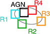 |
Fig. 1. Selected |

Coordinates (RA and Dec) of the five selected regions within the CND.
Figures 2–5 show the spectra for all transitions used in this study in unit of [K], with all the [mJy beam−1] to [K] conversion factors listed in Table 1, from the five selected positions listed in Table 2. The observed HNCO(4–3) and (5–4) spectra are in Fig. 2, HNCO(6–5) and SiO(2–1) spectra in Fig. 3, SiO(3–2) and SiO(5–4) in Fig. 4, and SiO(6–5) and SiO(7–6) in Fig. 5. These spectral data are extracted from the data cube in their own original spatial and spectral resolution, and then averaged over a common-size aperture of  box centering at each selected position. All the adjacent bonus lines are also displayed, labeled by the blue dashed vertical lines in the spectra – as opposed to the targeted HNCO and SiO lines in blue, solid vertical lines (including the splittings). Based on the strongest spectral line features in all transitions, the estimated line width is about 100 km s−1, which is slightly smaller but consistent with the estimate of the line width in the CND region of NGC 1068 from previous studies (Kelly et al. 2017).
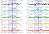 |
Fig. 2. Spectra of the HNCO (4–3) and HNCO (5–4) transitions. Each color-coded solid curve plots the spectral data from each selected |

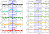 |
Fig. 3. Spectra of the HNCO (6–5) and SiO (2–1) transitions. Each color-coded solid curve plots the spectral data from each selected |

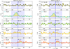 |
Fig. 4. Spectra of the SiO (3–2) and SiO(5–4) transitions. Each color-coded solid curve plots the spectral data from each selected |

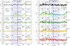 |
Fig. 5. Spectra of the SiO (6–5) and SiO (7–6) transitions. Each color-coded solid curve plots the spectral data from each selected |

The spot CND-R1 which is at the east-side of CND shows a very strong signal across all SiO transitions, and this is in contrast to the rest of CND where the SiO emission is much weaker. On the other hand, HNCO is much more evenly distributed throughout the CND. This will be more obvious in the intensity maps presented later in Sect. 3.2, and is in broad agreement with the findings from the lower-resolution observations towards the AGN-host galaxy NGC 1097 (Martín et al. 2015). For all three HNCO transitions there is prominent line emission on both sides (east and west) of the CND.
3.2. Moment-0 maps
Figure 6 shows the velocity-integrated intensity maps at each original spatial resolution of HNCO(4–3), HNCO(5–4), and HNCO(6–5) at the CND scale. Figure 7 shows the velocity-integrated intensity maps at the original spatial resolution for SiO(2–1), SiO(3–2), SiO(5–4), SiO(6–5), and SiO(7–6) at the CND scale. These line-intensity maps were integrated over velocity, and a 3.0σ threshold clipping was applied to the moment-0 maps. The line fluxes were integrated to include any significant emission that arises over the velocity span due to rotation and outflow motions in NGC 1068. Here, we used  km s−1 to cover such range, except for lines that have adjacent transitions which are covered by such a velocity span. In the latter case, which involves potential line contamination, the velocity integration was performed in a narrower range to the midpoint between the target line and the adjacent line, instead of performing further spectral fitting in an attempt to disentangle the multiple molecular transitions, for two reasons: (1) HNCO transitions actually involve multiple splitting components per transition (e.g., HNCO (4–3) line), which makes it much more complicated for the spectral fitting; and (2) there is no serious overlapping or contamination over different molecular transitions, thus narrowing the velocity range was acceptable for our purpose. For the HNCO transitions that involve multiple fine or hyperfine splittings, the velocity is referring to the frequency associated with the expected strongest component. Those lines with narrowed velocity coverage are: HNCO(5–4) with [−230 km s−1, 167 km s−1], SiO(2–1) with [−230 km s−1, 160 km s−1], SiO(6–5) with [−230 km s−1, 151 km s−1], and SiO(7–6) with [−74 km s−1, 230 km s−1]. The velocity covered to derive the velocity-integrated line intensities are also displayed in shaded blue in the individual spectra shown in Figs. 2–5. We note that the chosen velocity range may cover multiple gas components, as in the double-peak feature in CND-R3 of both HNCO(5–4) (middle panel) and HNCO(6–5) (right panel) in Figs. 2–3. For the purposes of this study, we simply aim to investigate the properties of the averaged gas within the beam.
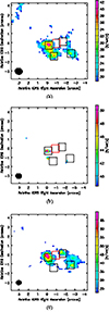 |
Fig. 6. The velocity-integrated intensity maps of (a) HNCO(4–3), (b) HNCO(5–4), and (c) HNCO(6–5) at their original spatial resolution. The black and red boxes mark the regions listed in Table 2, where AGN is marked with the red box. These maps are masked with a 3.0σ threshold after the integration over velocity. The integrated velocity range for HNCO(4–3) and HNCO(6–5) are [−230 km s−1, 230 km s−1], and HNCO(5–4) with [−230 km s−1, 167 km s−1] so that to exclude the nearby line. |
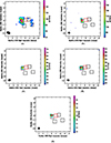 |
Fig. 7. The velocity-integrated intensity maps of (a) SiO(2–1), (b) SiO(3–2), (c) SiO(5–4), (d) SiO(6–5), (e) SiO(7–6) at their original spatial resolution. This is zoomed-in at the CND scale. The black and red boxes mark the regions listed in Table 2, where the AGN is marked with the red box. These maps are masked with a 3.0σ threshold after the integration over velocity. The velocity ranges for integration are: SiO(2–1) with [−230 km s−1, 160 km s−1], SiO(6–5) with [−230 km s−1, 151 km s−1], and SiO(7–6) with [−74 km s−1, 230 km s−1], and for the rest is the default [−230 km s−1, 230 km s−1]. |
The CND ring structure traced by HNCO and SiO in the velocity-integrated intensity maps is noticeably off-centered from the inferred location of the AGN in the literature (Roy et al. 1998; García-Burillo et al. 2014), but coincides with the CO observations at similar and higher spatial resolution (García-Burillo et al. 2014, 2019; Viti et al. 2014), dust continuum (García-Burillo et al. 2014), and observations of the dense gas tracers such as HCN and HCO+ (Krips et al. 2011; García-Burillo et al. 2014; Imanishi et al. 2016). The contribution from atomic hydrogen to the total neutral gas content is negligible in the central ∼2 kpc of the disk (Brinks et al. 1997; García-Burillo et al. 2014, 2017) compared to the molecular counterpart. This off-centered ring morphology could be an indication that the ring is possibly being shaped by the feedback of nuclear activity (García-Burillo et al. 2019). Moreover, the CND ring revealed by our HNCO and SiO emissions shows substructure with several knots along the ring morphology. At the CND, the emission from all the transitions peaks near the R1 region. In particular for HNCO(6–5), such a trend is in contrast to what was found in the previous work by Kelly et al. (2017), where the strongest HNCO(6–5) peaked at the CND west side. The strongest HNCO(6–5) emission (69.79 K km s−1) is in the east of the CND, and this intensity is comparable to the peak intensity of the HNCO(6–5) emission of 60 K km s−1 reported by Kelly et al. (2017), although the latter occurred in the west of the CND. The peak emission of HNCO(4–3) and HNCO(5–4) are also at the east side of CND, at 42.41 K km s−1 and 50.73 K km s−1, respectively.
Compared to the SiO transitions, which are mostly centered around CND-R1, the HNCO(4–3), and HNCO(6–5) emission appears to be more evenly extended to the west side throughout the entire CND. This is indeed similar to the findings of Martín et al. (2015) obtained from lower-resolution observations towards NGC 1097, where HNCO was found to be more extended on its CND, and SiO was found more likely as an unresolved source.
The two emission knots (east and west) are connected by a “bridge” structure of weaker emission that can be seen on both the north and south side of the AGN. In both HNCO(4–3) and HNCO(6–5) there are several local knots in this “bridge” that are part of the CND ring (e.g., CND-R2 and CND-R4). Intriguingly, HNCO(4–3) shows more prominent “bridge” emission in the south bridge, while HNCO(6–5) appears more prominent in the north bridge. HNCO(5–4) also shows comparable emission on both sides of the CND; however, likely due to the higher noise level for this data set, most of the regions are below the threshold.
3.3. Molecular line ratios and overlay maps
In this section, we analyze selected line ratios at our observed locations in the CND of NGC 1068. Prior to deriving the ratio and overlay maps, all the unmasked line intensity maps were smoothed2 to the lowest common resolution across the data,  , re-projected to the same spatial grids3 in order to have a consistent map coordinate, and then we masked out pixels below the 3.0σ threshold for further image analysis. In general, the noise will also be suppressed when performing the image smoothing and some weak signals may reach the cutoff threshold (e.g. 3.0σ). Hence, we first smooth and re-project the unmasked intensity maps, followed by the re-sampling of the noise and the mask application on the new images. From this section onward, all the data products have been spatially degraded to this common resolution (
 ) and processed according to the description above for all transitions.
Differences in line intensity ratios can arise from several physical processes, such as differences in systematic gas density and temperature, different radiation fields (e.g., UV, X-rays), and the presence and type of shocks (see detailed discussion in Krips et al. 2008). Therefore, molecular ratios can be powerful diagnostics in determining the physical characteristics as well as the energetic processes of a galaxy. In Sect. 3.2, we highlighted that the HNCO transitions appear to be more evenly distributed over all CND regions, in contrast to the SiO emission which is mostly in the East-CND region. By inspecting both molecular-line ratio maps and overlay maps, we aim to systematically compare such differences between the two molecular tracers in a morphological and quantitative way. Quantitatively, the uncertainty of the intensity ratio can be estimated through standard error propagation from the uncertainty measured in the line intensity in the ideal case. With a threshold ≥3.0σ for the quantities involved, the uncertainty of the ratio is ≤47% of the ratio itself. We note that for ratios near 1.0, such an uncertainty may reverse the ratio from below to above 1 (or vice versa).
In Figs. 8 to 10 we highlight few transition “pairs”, namely: HNCO(4–3)/HNCO(5–4)/HNCO(6–5) versus SiO(3–2) to show both the molecular line ratio and overlay maps of the velocity-integrated intensities in ∫Tmb ⋅ dv (K km s−1). The rest of the SiO/HNCO ratios show similar trends. The selected transition pairs are few of the most prominent examples demonstrating the trend in line ratios from the east to the west of the CND. In particular, we chose to show the ratio HNCO(6–5)/SiO(3–2), as this was the ratio that was modelled in Kelly et al. (2017) in an attempt to characterize the gas properties traced by these two molecular species. In the work by Kelly et al. (2017), the PdBI observations of the HNCO(6–5) and SiO(3–2) transitions were compared and it was found that in the overlay map (Fig. 4 in Kelly et al. 2017), there is a noticeable spatial offset in the both east and west local peaks between these two transitions. As shown in Fig. 10, we find that for the same transition pair, the spatial offset between the HNCO(6–5) and SiO(3–2) peak emissions on both east and west CND is actually not as large as (both  ) identified in Kelly et al. (2017), which reported it to be
  .
.
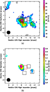 |
Fig. 8. The comparison maps between SiO(3–2) and HNCO(4–3) in overlay and ratio maps. In the overlay (a) map the HNCO(4–3) is shown in color map, and SiO(3–2) in contours. The contour starts from 3.0σ, with step of 3.0σ. In (b) the SiO(3–2)/HNCO(4–3) ratio map is displayed. The black and red square boxes mark the |


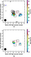 |
Fig. 9. The comparison maps between SiO(3–2) and HNCO(5–4) in overlay and ratio maps. In the overlay (a) map the HNCO(5–4) is shown in color map, and SiO(3–2) in contours. The contour starts from 3.0σ, with step of 3.0σ. In (b) the SiO(3–2)/HNCO(5–4) ratio map is displayed. The black and red square boxes mark the |


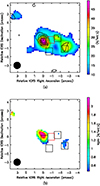 |
Fig. 10. The comparison maps between SiO(3–2) and HNCO(6–5) in overlay and ratio maps. In the overlay (a) map the HNCO(6–5) is shown in color map, and SiO(3–2) in contours. The contour starts from 3.0σ, with step of 3.0σ. In (b) the SiO(3–2)/HNCO(6–5) ratio map is displayed. The black and red square boxes mark the |


On the other hand, the general SiO(3–2)/HNCO ratios do show a noticeable gradient on the plane of sky across the CND, going from ≥1.0 on the east side to ≤1.0 on the west side. This confirms the same trend of chemical differentiation highlighted by Kelly et al. (2017) across the CND, which may arise from their different chemical “origins” such as the shock chemistry involved in different types of shocks, for instance, fast and slow shocks. This may indicate different velocity regimes in the shock fronts of the molecular outflow. As mentioned earlier, Kelly et al. (2017) performed a chemical modeling for the SiO and HNCO emission, and confirmed that fast shocks (60 km s−1) are likely to be producing SiO; while HNCO can be associated with slow-shock (20 km s−1) chemistry, or simply with the mantle sublimation in the gas that is warm, dense, and non-shocked. A further characterization of the gas properties will be the key to verifying the perspective provided by the chemical modeling and to disentangling the gas condition traced by HNCO.
4. Characterizing the physical properties of the gas in the CND
The relative configuration of the CND to the geometry of the jet-ISM interaction and the outflow provides us with the opportunity to explore shock-driven chemistry related to the molecular outflow, for the large spread of velocities is likely driving different shock chemistry signatures at different locations in the CND (García-Burillo et al. 2014, 2017; Viti et al. 2014; Kelly et al. 2017). One of our main goals in the current work is to better characterize the gas properties that SiO and HNCO each traces across the CND regions, using a larger number of transitions, observed at a higher spatial resolution ( ) than in the previous study (∼1″ − 4″) by Kelly et al. (2017). Ultimately, we explore whether the observed SiO-HNCO properties can be used as a keen probe to the variation of the shocked gas properties across the CND.
To characterize the SiO and HNCO emissions across the CND region, we performed: (i) an LTE analysis (Sect. 4.1) and (ii) a radiative analysis via radiative transfer modeling (Sect. 4.2). The main goal is to characterize the column density of each molecular species and, more importantly, the gas temperature and the gas density in the CND. For reference, Table 3 also lists all the measured velocity-integrated line intensities (in K km s−1) from the observations smoothed to the common resolution of  .
.
Velocity-integrated line intensity of HNCO and SiO transition covered in the current work.
4.1. LTE analysis
In quantifying the physical conditions probed by our HNCO and SiO transitions, we first performed a basic LTE analysis. We calculated the total column density (N) of a given species via the Boltzmann equation in LTE at temperature Tk:
 (1)
(1)
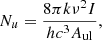
where N is the total column density of the species, Nu is the column density of the upper level, u, and Z is the partition function, gu is the statistical weight of the level u, and Eu is its energy above the ground state. The molecular column density at upper level u, namely, Nu, can be related to the observed integrated line intensity from any given transition, assuming optically thin and a filling factor of unity:
 (2)
(2)
where I = ∫Tmb ⋅ dv is the integrated line intensity (in K km s−1) over the spectral axis. In general, the formalism above provides a lower limit for the true N. This is because, in a more realistic setup, we would also need to consider an opacity correction factor in Eq. (2), which would underestimate the N in Eq. (1); however, such correction can be neglected under an optically thin condition (Goldsmith & Langer 1999). The HNCO column densities inferred from its three transitions are generally consistent within one order of magnitude, and by using temperature Tk = 50 − 200 K, the HNCO column density is between 4 × 10¹⁴ − 9.5 × 1015 cm−2 among the CND regions. However, the inferred column density of SiO greatly varies among the available transitions. With temperatures of Tk = 50 − 200 K, the SiO column density is between 6.5 × 10¹² − 2.1 × 1015 cm−2. The temperature span, Tk = 50 − 200 K, that is explored here is based on the previously inferred gas temperature by Viti et al. (2014) and Kelly et al. (2017) in the CND.
In order to constrain the temperature, we can also construct the rotation diagram that relates the quantity ln(Nu/gu) to the Eu linearly with a slope of ( − 1/Trot), given that we are mostly in the Rayleigh-Jeans scenario and since we have multiple transitions for each species per selected region. The rotational temperature, Trot, is expected to be equal to kinetic temperature, Tkin, if all levels are thermalized (Goldsmith & Langer 1999), and it can generally be used as a lower limit estimate for Tkin.
Figure 11 shows the rotation diagrams with the uncertainty constructed across the five CND regions, color coded accordingly, using all available transitions from HNCO and SiO, respectively. The uncertainties are the propagated error estimate from the measured line intensities.
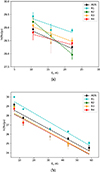 |
Fig. 11. The rotation diagram derived from (a) HNCO transitions and (b) SiO transitions in all selected regions. The uncertainty is propagated from the measured error from the line intensity. The color coding indicates data from each region selected as shown in the schematic in Fig. 6d. The faded (gray-ish) marks indicate data points below 3.0σ cut, to which case we will use 3.0σ as upper limit in our further analysis. The fitted rotational temperature are list in Table A.1. |
The inferred Trot for HNCO is between 9 − 30 K, and for SiO it is between 11 − 12 K. The individual fitted Trot values are listed in Table A.1. The fitting for HNCO is generally within the uncertainties of the line intensities. On the other hand, for SiO transitions, the linear fit is generally not well constrained within the errors of the data points, which is consistent with the fact that the column densities derived from different transitions significantly differ at a fixed temperature. Taking CND-R1 region as the most prominent example, a one-component fit is not especially convincing. Thus, it is indeed likely that different transitions may not always trace the same gas components. Aside from the potential multiplicity of gas components within our beams, Goldsmith & Langer (1999) and Martín et al. (2019) showed that both the opacity and the gas density each transition is tracing can lead to deviations from a linear fit in the rotation diagram. In fact, based on our RADEX analysis (Sect. 4.2), it is possible for lower-J SiO transition (2–1 and 3–2) to transit into the optically thick regime, where the optical depth can be as high as ∼10, when the molecular gas density goes below 104 − 5 cm−3. This could contribute to the non-linearity shown in the SiO rotation diagram. When the molecular gas density (nH2) goes below the critical density (ncrit) of the given transition, the emission that is not thermalized will also break the linearity. This is discussed further in Sect. 4.2 and Appendix C.
In summary, the main take-away point from the rotation diagrams is that, even within each sub-region of the CND, the gas traced by SiO is not well characterized by a single gas component with LTE condition, which is indeed consistent with such gas being heavily shocked and the fact that a gradient of gas conditions may be present. This is also consistent with the findings by Viti et al. (2014), where they concluded that gas within the same selected region of the CND is not well characterized by a single gas phase. In order to further test whether the gas is in LTE, we performed a non-LTE analysis (presented in the next section).
4.2. Non-LTE analysis with RADEX
For the non-LTE analysis, we use the radiative transfer code RADEX (van der Tak et al. 2007) via the Python package SpectralRadex4 (Holdship et al. 2021) using HNCO and SiO molecular data (Niedenhoff et al. 1995; Sahnoun et al. 2018; Balança et al. 2018) from the LAMDA database (Schöier et al. 2005). This allows us to account for how the gas density and temperature affect the excitation of the transitions and to fit three parameters of interest: nH2, Tkin, and N as well as the beam filling factor.
In order to properly sample this parameter space and obtain reliable uncertainties, we coupled the RADEX modeling with the Markov chain Monte Carlo (MCMC) sampler emcee (Foreman-Mackey et al. 2013) to perform a Bayesian inference of the parameter probability distributions. We assumed uniform priors within the determined ranges (given in Table 4) and agreed that the uncertainty on our measured intensities is Gaussian so that our posterior distribution is given by  where χ2 is the chi-squared statistic between our measured intensities and the RADEX output for a set of parameters θ. We include the intensities of all transitions in our observed frequency range, even those that fall below 3.0σ. These non-detected transitions still contribute information because our modeling approach assumes the integrated intensity contains only molecular emission plus noise. If the molecular emission is weak enough for the noise to dominate, a well fitting model should predict that result.
In general this analysis is confined by the assumption that all of the molecular transitions arise from a single, homogeneous gas component. However, this assumption is crude and can only offer an averaged point of view for the gas properties given the limited resolution provided by observations, the different critical densities of the available transitions, and the energetic conditions required for each chemical species. Despite that, if variations in gas temperature and density within each sub-region of the CND are not too steep, a RADEX analysis should still be able to give us an indication of the average gas properties in the non-LTE study.
Based on the chemical modeling performed by Kelly et al. (2017), which suggested that SiO and HNCO are probing different shock scenarios (fast versus slow shocks), and, thus, potentially very different gas properties, we chose to separate these two species in our RADEX analysis and infer the gas properties for each species individually. In Figs. 12–15, we show the posterior parameter distributions obtained for HNCO (green) and SiO (blue) for each of the four selected CND regions (R1–R4). The most likely values for these parameters are also listed in Table 5, with the uncertainties calculated by taking an interval around the most likely value that contains 67% of the probability density, similar to a 1σ uncertainty. The corner plots for individual species per region can also be found in the Appendix B.1. We note that we do not include the analysis for AGN, as the signal from AGN is mostly below the 3.0σ threshold, which is probably the result of beam smearing with the current resolution 0.8″.
 |
Fig. 12. Bayesian inference results for gas properties traced by HNCO (green) and SiO (blue) of CND-R1 region. The corner plots show the sampled distributions for each parameter, as displayed on the x-axis. The 1D distributions on the diagonal are the posterior distributions for each explored parameter; the reset 2D distributions are the joint posterior for corresponding parameter pair on the x- and y- axes. In the 1D distributions, the 1σ regions are shaded with blue; both 1σ and 2σ are shaded in the 2D distributions. |
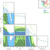 |
Fig. 13. As in Fig. 12 but for the CND-R2 region. This shows the Bayesian inference results for gas properties traced by HNCO (green) and SiO (blue) of CND-R2 region. |
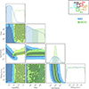 |
Fig. 14. As in Fig. 12 but for the CND-R3 region. This shows the Bayesian inference results for gas properties traced by HNCO (green) and SiO (blue) of CND-R3 region. |
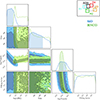 |
Fig. 15. As in Fig. 12 but for the CND-R4 region. This shows the Bayesian inference results for gas properties traced by HNCO (green) and SiO (blue) of CND-R4 region. |
Inferred gas properties traced by HNCO and SiO from the Bayesian inference processes over four selected regions across CND (R1–R4).
The gas conditions derived from the SiO emission present an interesting case. In each region, the gas density posterior strongly favours values less than 5 × 104 cm−3. This is consistent with the density range found in the chemical modelling of Kelly et al. (2017) in which a fast shock is needed to enhance the SiO abundance. However, in R1 and R2 which have detections with higher signal-to-noise ratios (S/N), the posterior actually peaks at the lowest value allowed by the prior. Thus, the fit appears to strongly favour extremely low densities. At the same time, the gas temperature is unconstrained in every case except R1, for which we obtained a temperature of  K. Compared to previous observations, the extremely low density values do not appear to be physical; for instance, SiO was found to trace a higher gas density of ∼105 cm−3 by Usero et al. (2004) and García-Burillo et al. (2010) using lower resolution observations toward the CND of NGC 1068. As the physical scale we are studying (
 pc) is comparable to GMCs scales, we also compared our results to the gas density as traced by SiO from the nucleus of our own galaxy: Hüttemeister et al. (1998) surveyed 33 sources in the Galactic center region at pc-scale resolution and invoked shocks as the process responsible for the enhanced SiO abundance. Using the SiO and 29SiO line ratios, they found that SiO traces hot (T > 100 K) and thin (nH2∼ a few 103 cm−3) gas. In fact, our measured gas density is quite close to the density described by Hüttemeister et al. (1998), although we want to stress that our model seems to prefer the lowest possible density (towards 102 cm−3), which is even lower than the density inferred by Hüttemeister et al. (1998). On the other hand, the only constrained temperature (for R1) is supported by a multiple-species RADEX analysis of dense gas tracers by Viti et al. (2014), where the temperature was found to be > 400 K. This finding is also consistent with prior lower-resolution data from Krips et al. (2011).
We therefore recommend caution when interpreting the gas density values inferred from the SiO emission. A variety of gas conditions are expected in a shocked environment, which may lead to relative excitation between transitions that cannot be captured with a single RADEX component (as discussed in Sect. 4.1). In fact, we have estimated the critical densities of the SiO transitions for the purposes the current work with a temperature of T ∈ (10, 800) K (as listed in Table C.1) and found that the inferred gas densities from RADEX analysis traced by SiO are actually below the critical density. It may therefore be the case that the only way to obtain a reasonable fit with a single component is to combine very low densities to produce sub-thermal excitation and then very high temperatures to excite the low Eu transitions, as we have observed. These conditions would not therefore be representative of any kind of average conditions in the region.
The best fit for the gas density traced by HNCO is not well constrained overall, but it has a lower limit of 104 cm−3 in every region except for CND-R2 where lower densities are favoured. No constraint on the gas temperature from the HNCO emission is found in any case. From these physical parameters, we can consider the enhancement mechanism of HNCO. The abundance of HNCO is found to be enhanced in the presence of slow shocks for initial gas densities in the range 103 − 5 cm−3 or in a shock-free but warm and dense (> 104 cm−3) environment (Kelly et al. 2017). At low gas density (103 cm−3) the molecular gas and the dust are not coupled, therefore the dust temperature will be lower than the gas temperature, and at this density the dust grain mantles are not sublimated unless shock sputtering occurs. At higher densities, gas and dust are coupled and, hence, the mantles can be sublimated without the presence of shock. For the shock-free scenario, therefore, higher gas density is required for HNCO enhancement. Hence, we conclude that for nearly all regions (except for CND-R2), the enhancement of HNCO can be just a consequence of the environment being hotter than the sublimation temperature of HNCO; however, if we are to believe that the gas density in CND-R2 is, on average, as low as 102 cm−3, then the only way to enhance HNCO is via shock sputtering.
The molecular column densities per species are well constrained in most regions except for CND-R2. The SiO column density generally ranges from 1014 − 17 cm−2 (except for CND-R2, where it is much lower, namely, ∼1012 cm−2); this is comparable but generally larger than the LTE-based estimate of SiO column density presented in Sect. 4.1. The HNCO column density is approximately 1015 cm−2 in every case, and this is quite consistent with the LTE values derived in Sect. 4.1. We may speculate that these results are consistent with the gas traced by SiO being strongly affected by shocks (and, hence, unlikely to be in LTE), whereas the gas traced by HNCO may be closer to LTE.
5. Conclusions
The molecular gas in the CND of NGC 1068 is outflowing, likely a manifestation of ongoing AGN feedback (García-Burillo et al. 2014, 2019). As the outflowing gas has a large spread of velocities (∼100 km s−1), which likely drive a range of different shocks at different locations in the CND, we perform a multi-line molecular study with ALMA of two typical shock tracers in order to determine the chemical signatures of such shocks. In particular, we analyze three HNCO lines and five SiO lines of the nearby galaxy NGC 1068 at spatial resolution of  . We briefly summarize our conclusions below:
-
For both species, the strongest peaks all occur on the east side of the circumnuclear disk (CND), which is not consistent with the lower spatial resolution observations by Kelly et al. (2017), where they found that HNCO(6–5) peaks in the west of the CND. The cross-species ratio maps of velocity-integrated line intensities of SiO and HNCO, however, show clear spatial differentiation going from large SiO/HNCO ratios in the east to a low SiO/HNCO ratio in the west of the CND; this is consistent with the trend identified in Kelly et al. (2017).
-
We performed LTE and non-LTE analyses. For the latter, we coupled a radiative transfer analysis using RADEX with a Bayesian inference procedure, in order to infer the gas properties traced by these two species. The inferred gas densities traced by SiO are generally constrained to be less than 5 × 104 cm−3 and they are consistent with a scenario where strong shocks (≥ 50 kms−1) are present. The inferred gas densities traced by HNCO, however, are not as well constrained overall but tend toward a higher gas density (≥104 cm−3); with the exception of CND-R2, where the gas density seems to below 104 cm−3. The low inferred gas density in CND-R2 would require the presence of slow shocks (∼20 km s−1) to produce the observed HNCO. We cannot draw the same conclusion for the regions where HNCO yield a higher gas density.
-
Our work indicates that SiO and HNCO trace different gas components within the beam and, most importantly, different shock conditions and histories. This result is in agreement with previous studies. To further disentangle the gas conditions traced by HNCO will require future observations that cover more HNCO transitions at comparable spatial resolution to complete the current investigation.
Using CASA task “imsmooth” with parameter “targetres = True” specified to used the indicated beam geometry as the final aimed, the lower “common” resolution shared in any given transition pair.
Using CASA task “imregrid”.
Acknowledgments
KYH, SV, and JH are funded by the European Research Council (ERC) Advanced Grant MOPPEX 833460.vii. SGB acknowledges support from the research project PID2019-106027GA-C44 of the Spanish Ministerio de Ciencia e Innovación. KK acknowledges the support by JSPS KAKENHI Grant Number JP17H06130 and the NAOJ ALMA Scientific Research Grant Number 2017-06B. MSG acknowledges support from the Spanish Ministerio de Economía y Competitividad through the grants BES-2016-078922, ESP2017-83197-P and the research project PID2019-106280GB-100. KYH acknowledges assistance from Allegro, the European ALMA Regional Center node in the Netherlands. This paper makes use of the following ALMA data: ADS/JAO.ALMA#2013.1.00221.S, ADS/JAO.ALMA#2015.1.01144.S, and ADS/JAO.ALMA#2018.1.01506.S. ALMA is a partnership of ESO (represent- ing its member states), NSF (USA) and NINS (Japan), together with NRC (Canada), MOST and ASIAA (Taiwan), and KASI (Republic of Korea), in co operation with the Republic of Chile. The Joint ALMA Observatory is operated by ESO, AUI/NRAO and NAOJ.
References
- Aladro, R., Martín-Pintado, J., Martín, S., Mauersberger, R., & Bayet, E. 2011, A&A, 525, A89 [NASA ADS] [CrossRef] [EDP Sciences] [Google Scholar]
- Aladro, R., Viti, S., Bayet, E., et al. 2013, A&A, 549, A39 [NASA ADS] [CrossRef] [EDP Sciences] [Google Scholar]
- Balança, C., Dayou, F., Faure, A., Wiesenfeld, L., & Feautrier, N. 2018, MNRAS, 479, 2692 [Google Scholar]
- Bayet, E., Lintott, C., Viti, S., et al. 2008, ApJ, 685, L35 [NASA ADS] [CrossRef] [Google Scholar]
- Bland-Hawthorn, J., Gallimore, J. F., Tacconi, L. J., et al. 1997, Ap&SS, 248, 9 [Google Scholar]
- Brinks, E., Skillman, E. D., Terlevich, R. J., & Terlevich, E. 1997, Ap&SS, 248, 23 [NASA ADS] [CrossRef] [Google Scholar]
- Draine, B. T. 2011, Physics of the Interstellar and Intergalactic Medium (Princeton University Press) [Google Scholar]
- Fedoseev, G., Ioppolo, S., Zhao, D., Lamberts, T., & Linnartz, H. 2015, MNRAS, 446, 439 [NASA ADS] [CrossRef] [Google Scholar]
- Foreman-Mackey, D., Hogg, D. W., Lang, D., & Goodman, J. 2013, PASP, 125, 306 [Google Scholar]
- Gao, Y., & Solomon, P. M. 2004, ApJ, 606, 271 [NASA ADS] [CrossRef] [Google Scholar]
- García-Burillo, S., Martín-Pintado, J., Fuente, A., & Neri, R. 2000, A&A, 355, 499 [NASA ADS] [Google Scholar]
- García-Burillo, S., Martín-Pintado, J., Fuente, A., Usero, A., & Neri, R. 2002, ApJ, 575, L55 [CrossRef] [Google Scholar]
- García-Burillo, S., Usero, A., Fuente, A., et al. 2010, A&A, 519, A2 [NASA ADS] [CrossRef] [EDP Sciences] [Google Scholar]
- García-Burillo, S., Combes, F., Usero, A., et al. 2014, A&A, 567, A125 [Google Scholar]
- García-Burillo, S., Viti, S., Combes, F., et al. 2017, A&A, 608, A56 [Google Scholar]
- García-Burillo, S., Combes, F., Ramos Almeida, C., et al. 2019, A&A, 632, A61 [Google Scholar]
- Gerin, M., Goicoechea, J. R., Pety, J., & Hily-Blant, P. 2009, A&A, 494, 977 [NASA ADS] [CrossRef] [EDP Sciences] [Google Scholar]
- Goldsmith, P. F., & Langer, W. D. 1999, ApJ, 517, 209 [Google Scholar]
- Hailey-Dunsheath, S., Sturm, E., Fischer, J., et al. 2012, ApJ, 755, 57 [NASA ADS] [CrossRef] [Google Scholar]
- Holdship, J., Viti, S., Martín, S., et al. 2021, A&A, 654, A55 [NASA ADS] [CrossRef] [EDP Sciences] [Google Scholar]
- Hüttemeister, S., Dahmen, G., Mauersberger, R., et al. 1998, A&A, 334, 646 [NASA ADS] [Google Scholar]
- Imanishi, M., Nakanishi, K., & Izumi, T. 2016, ApJ, 822, L10 [Google Scholar]
- Imanishi, M., Nguyen, D. D., Wada, K., et al. 2020, ApJ, 902, 99 [CrossRef] [Google Scholar]
- Impellizzeri, C. M. V., Gallimore, J. F., Baum, S. A., et al. 2019, ApJ, 884, L28 [NASA ADS] [CrossRef] [Google Scholar]
- Israel, F. P. 2009, A&A, 493, 525 [NASA ADS] [CrossRef] [EDP Sciences] [Google Scholar]
- Jiménez-Serra, I., Caselli, P., Martín-Pintado, J., & Hartquist, T. W. 2008, A&A, 482, 549 [NASA ADS] [CrossRef] [EDP Sciences] [Google Scholar]
- Kamenetzky, J., Glenn, J., Maloney, P. R., et al. 2011, ApJ, 731, 83 [NASA ADS] [CrossRef] [Google Scholar]
- Kauffmann, J., Goldsmith, P. F., Melnick, G., et al. 2017, A&A, 605, L5 [NASA ADS] [CrossRef] [EDP Sciences] [Google Scholar]
- Kelly, G., Viti, S., García-Burillo, S., et al. 2017, A&A, 597, A11 [NASA ADS] [CrossRef] [EDP Sciences] [Google Scholar]
- Krips, M., Neri, R., García-Burillo, S., et al. 2008, ApJ, 677, 262 [NASA ADS] [CrossRef] [Google Scholar]
- Krips, M., Martín, S., Eckart, A., et al. 2011, ApJ, 736, 37 [NASA ADS] [CrossRef] [Google Scholar]
- López-Sepulcre, A., Jaber, A. A., Mendoza, E., et al. 2015, MNRAS, 449, 2438 [CrossRef] [Google Scholar]
- Martín, S., Requena-Torres, M. A., Martín-Pintado, J., & Mauersberger, R. 2008, ApJ, 678, 245 [CrossRef] [Google Scholar]
- Martín, S., Martín-Pintado, J., & Mauersberger, R. 2009a, ApJ, 694, 610 [CrossRef] [Google Scholar]
- Martín, S., Martín-Pintado, J., & Viti, S. 2009b, ApJ, 706, 1323 [Google Scholar]
- Martín, S., Kohno, K., Izumi, T., et al. 2015, A&A, 573, A116 [NASA ADS] [CrossRef] [EDP Sciences] [Google Scholar]
- Martín, S., Martín-Pintado, J., Blanco-Sánchez, C., et al. 2019, A&A, 631, A159 [Google Scholar]
- Martín-Pintado, J., de Vicente, P., Fuente, A., & Planesas, P. 1997, ApJ, 482, L45 [NASA ADS] [CrossRef] [Google Scholar]
- McMullin, J. P., Waters, B., Schiebel, D., Young, W., & Golap, K. 2007, in Astronomical Data Analysis Software and Systems XVI, eds. R. A. Shaw, F. Hill, & D. J. Bell, ASP Conf. Ser., 376, 127 [Google Scholar]
- Meier, D. S., & Turner, J. L. 2005, ApJ, 618, 259 [NASA ADS] [CrossRef] [Google Scholar]
- Meier, D. S., & Turner, J. L. 2012, ApJ, 755, 104 [NASA ADS] [CrossRef] [Google Scholar]
- Meier, D. S., Walter, F., Bolatto, A. D., et al. 2015, ApJ, 801, 63 [NASA ADS] [CrossRef] [Google Scholar]
- Niedenhoff, M., Yamada, K. M. T., Belov, S. P., & Winnewisser, G. 1995, J. Mol. Spectrosc., 174, 151 [NASA ADS] [CrossRef] [Google Scholar]
- Pety, J., Guzmán, V. V., Orkisz, J. H., et al. 2017, A&A, 599, A98 [NASA ADS] [CrossRef] [EDP Sciences] [Google Scholar]
- Rodríguez-Fernández, N. J., Tafalla, M., Gueth, F., & Bachiller, R. 2010, A&A, 516, A98 [Google Scholar]
- Roy, A. L., Colbert, E. J. M., Wilson, A. S., & Ulvestad, J. S. 1998, ApJ, 504, 147 [NASA ADS] [CrossRef] [Google Scholar]
- Sahnoun, E., Wiesenfeld, L., Hammami, K., & Jaidane, N. 2018, J. Phys. Chem. A, 122, 3004 [NASA ADS] [CrossRef] [Google Scholar]
- Sánchez-García, M., García-Burillo, S., Pereira-Santaella, M., et al. 2022, A&A, 660, A83 [NASA ADS] [CrossRef] [EDP Sciences] [Google Scholar]
- Savage, C., & Ziurys, L. M. 2004, ApJ, 616, 966 [NASA ADS] [CrossRef] [Google Scholar]
- Schilke, P., Walmsley, C. M., Pineau des Forets, G., & Flower, D. R. 1997, A&A, 321, 293 [NASA ADS] [Google Scholar]
- Schinnerer, E., Eckart, A., Tacconi, L. J., Genzel, R., & Downes, D. 2000, ApJ, 533, 850 [Google Scholar]
- Schöier, F. L., van der Tak, F. F. S., van Dishoeck, E. F., & Black, J. H. 2005, A&A, 432, 369 [Google Scholar]
- Scoville, N. Z., Matthews, K., Carico, D. P., & Sanders, D. B. 1988, ApJ, 327, L61 [NASA ADS] [CrossRef] [Google Scholar]
- Usero, A., García-Burillo, S., Fuente, A., Martín-Pintado, J., & Rodríguez-Fernández, N. J. 2004, A&A, 419, 897 [NASA ADS] [CrossRef] [EDP Sciences] [Google Scholar]
- Usero, A., García-Burillo, S., Martín-Pintado, J., Fuente, A., & Neri, R. 2006, A&A, 448, 457 [NASA ADS] [CrossRef] [EDP Sciences] [Google Scholar]
- van der Tak, F. F. S., Black, J. H., Schöier, F. L., Jansen, D. J., & van Dishoeck, E. F. 2007, A&A, 468, 627 [NASA ADS] [CrossRef] [EDP Sciences] [Google Scholar]
- Viti, S. 2017, A&A, 607, A118 [NASA ADS] [CrossRef] [EDP Sciences] [Google Scholar]
- Viti, S., García-Burillo, S., Fuente, A., et al. 2014, A&A, 570, A28 [NASA ADS] [CrossRef] [EDP Sciences] [Google Scholar]
- Zinchenko, I., Henkel, C., & Mao, R. Q. 2000, A&A, 361, 1079 [NASA ADS] [Google Scholar]
Appendix A: Additional results from LTE analysis
Here, we attach some additional results from the rotation diagram described in Section 4.1. We performed single-component, linear fitting of the rotation diagram per species per region in order to constrain the rotational temperature (Trot) in each case. The results are shown in Table A.1
Single-component fitting of the rotational temperature described in Section 4.1.
Appendix B: Additional results from non-LTE analysis
B.1. Additional plots from RADEX analysis with Bayesian inference processes
In Figures B.1-B.2, we show the corner plots which shows the sampled distributions for each parameter. This is the same as in Figure 12-15, however, we plot each species individually instead of overlay the two species.
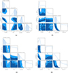 |
Fig. B.1. Corner plots which shows the sampled distributions for each parameter, as displayed on the x-axis. The 1D distributions on the diagonal are the posterior distributions for each explored parameter, the reset 2D distributions are the joint posterior for corresponding parameter pair on the x- and y- axes. In the 1D distributions, the 1σ regions are shaded with blue; both 1σ and 2σ are shaded in the 2D distributions. On top of each 1D distribution listed the inferred values if the distribution can be properly constrained. Results from CND-R1 and CND-R2 are presented: (a)SiO in CND-R1, (b) HNCO in CND-R1, (c)SiO in CND-R2, (d) HNCO in CND-R2 |
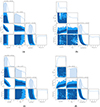 |
Fig. B.2. Same as Figure B.1, but for CND-R3 and CND-R4: (a)SiO in CND-R3, (b) HNCO in CND-R3, (c)SiO in CND-R4, (d) HNCO in CND-R4 |
B.2. Comparison of the predicted intensity from RADEX with observed values: A posterior predictive check (PPC)
In this section, we perform a posterior predictive check for the inferred gas properties in Section 4.2 using RADEX and Bayesian inference process. This is to verify our posterior distribution produces a distribution for the data that is consistent with the actual data, which is the velocity-integrated intensity in our case. We sample the predicted line intensities from our posterior between 16-84 percentile, and plot against the observed line intensities. The comparisons are shown in Figure B.3-B.4.
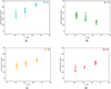 |
Fig. B.3. Observed and PPC intensities of HNCO for four CND regions: (a) CND-R1, (b) CND-R2, (c) CND-R3, (d) CND-R4. |
 |
Fig. B.4. Observed and PPC intensities of SiO for four CND regions: (a) CND-R1, (b) CND-R2, (c) CND-R3, (d) CND-R4. |
Appendix C: Critical density
We have noted that the inferred gas density, nH2, traced by SiO might be lower than the critical density at given temperature. Here, we give explicit estimates for the critical densities of SiO with gas temperature range from 10K to 800K. The critical density arises from the comparison of collisional deexcitation with radiative deexcitation (e.g., Draine 2011) and expressed as:
 (C.1)
(C.1)
where kuj is the collisional rate coefficient that bears a unit of [cm3 s-1] and can be turned into collisional rate [s-1] by multiplying volume density [cm-3]. Using SiO molecular data from LAMDA database (Schöier et al. 2005; Balança et al. 2018), we give estimate of SiO critical densities between T = 10K to 800K in Table C.1. It is clear that the inferred gas density traced by SiO in all CND regions (R1-R4) in Section 4.2 (102 − 4 cm-3) are all below even the lowest ncrit, 1.28 × 105 cm-3, among the temperature range and the transitions we explored.
Critical density of the SiO transitions used in current work at varying gas temperature.
All Tables
Observational details and the spatial resolution of the data used in this paper.
Velocity-integrated line intensity of HNCO and SiO transition covered in the current work.
Inferred gas properties traced by HNCO and SiO from the Bayesian inference processes over four selected regions across CND (R1–R4).
Single-component fitting of the rotational temperature described in Section 4.1.
Critical density of the SiO transitions used in current work at varying gas temperature.
All Figures
|
Fig. 1. Selected |
| In the text | |
|
Fig. 2. Spectra of the HNCO (4–3) and HNCO (5–4) transitions. Each color-coded solid curve plots the spectral data from each selected |
| In the text | |
|
Fig. 3. Spectra of the HNCO (6–5) and SiO (2–1) transitions. Each color-coded solid curve plots the spectral data from each selected |
| In the text | |
|
Fig. 4. Spectra of the SiO (3–2) and SiO(5–4) transitions. Each color-coded solid curve plots the spectral data from each selected |
| In the text | |
|
Fig. 5. Spectra of the SiO (6–5) and SiO (7–6) transitions. Each color-coded solid curve plots the spectral data from each selected |
| In the text | |
|
Fig. 6. The velocity-integrated intensity maps of (a) HNCO(4–3), (b) HNCO(5–4), and (c) HNCO(6–5) at their original spatial resolution. The black and red boxes mark the regions listed in Table 2, where AGN is marked with the red box. These maps are masked with a 3.0σ threshold after the integration over velocity. The integrated velocity range for HNCO(4–3) and HNCO(6–5) are [−230 km s−1, 230 km s−1], and HNCO(5–4) with [−230 km s−1, 167 km s−1] so that to exclude the nearby line. |
| In the text | |
|
Fig. 7. The velocity-integrated intensity maps of (a) SiO(2–1), (b) SiO(3–2), (c) SiO(5–4), (d) SiO(6–5), (e) SiO(7–6) at their original spatial resolution. This is zoomed-in at the CND scale. The black and red boxes mark the regions listed in Table 2, where the AGN is marked with the red box. These maps are masked with a 3.0σ threshold after the integration over velocity. The velocity ranges for integration are: SiO(2–1) with [−230 km s−1, 160 km s−1], SiO(6–5) with [−230 km s−1, 151 km s−1], and SiO(7–6) with [−74 km s−1, 230 km s−1], and for the rest is the default [−230 km s−1, 230 km s−1]. |
| In the text | |
|
Fig. 8. The comparison maps between SiO(3–2) and HNCO(4–3) in overlay and ratio maps. In the overlay (a) map the HNCO(4–3) is shown in color map, and SiO(3–2) in contours. The contour starts from 3.0σ, with step of 3.0σ. In (b) the SiO(3–2)/HNCO(4–3) ratio map is displayed. The black and red square boxes mark the |
| In the text | |
|
Fig. 9. The comparison maps between SiO(3–2) and HNCO(5–4) in overlay and ratio maps. In the overlay (a) map the HNCO(5–4) is shown in color map, and SiO(3–2) in contours. The contour starts from 3.0σ, with step of 3.0σ. In (b) the SiO(3–2)/HNCO(5–4) ratio map is displayed. The black and red square boxes mark the |
| In the text | |
|
Fig. 10. The comparison maps between SiO(3–2) and HNCO(6–5) in overlay and ratio maps. In the overlay (a) map the HNCO(6–5) is shown in color map, and SiO(3–2) in contours. The contour starts from 3.0σ, with step of 3.0σ. In (b) the SiO(3–2)/HNCO(6–5) ratio map is displayed. The black and red square boxes mark the |
| In the text | |
|
Fig. 11. The rotation diagram derived from (a) HNCO transitions and (b) SiO transitions in all selected regions. The uncertainty is propagated from the measured error from the line intensity. The color coding indicates data from each region selected as shown in the schematic in Fig. 6d. The faded (gray-ish) marks indicate data points below 3.0σ cut, to which case we will use 3.0σ as upper limit in our further analysis. The fitted rotational temperature are list in Table A.1. |
| In the text | |
|
Fig. 12. Bayesian inference results for gas properties traced by HNCO (green) and SiO (blue) of CND-R1 region. The corner plots show the sampled distributions for each parameter, as displayed on the x-axis. The 1D distributions on the diagonal are the posterior distributions for each explored parameter; the reset 2D distributions are the joint posterior for corresponding parameter pair on the x- and y- axes. In the 1D distributions, the 1σ regions are shaded with blue; both 1σ and 2σ are shaded in the 2D distributions. |
| In the text | |
|
Fig. 13. As in Fig. 12 but for the CND-R2 region. This shows the Bayesian inference results for gas properties traced by HNCO (green) and SiO (blue) of CND-R2 region. |
| In the text | |
|
Fig. 14. As in Fig. 12 but for the CND-R3 region. This shows the Bayesian inference results for gas properties traced by HNCO (green) and SiO (blue) of CND-R3 region. |
| In the text | |
|
Fig. 15. As in Fig. 12 but for the CND-R4 region. This shows the Bayesian inference results for gas properties traced by HNCO (green) and SiO (blue) of CND-R4 region. |
| In the text | |
|
Fig. B.1. Corner plots which shows the sampled distributions for each parameter, as displayed on the x-axis. The 1D distributions on the diagonal are the posterior distributions for each explored parameter, the reset 2D distributions are the joint posterior for corresponding parameter pair on the x- and y- axes. In the 1D distributions, the 1σ regions are shaded with blue; both 1σ and 2σ are shaded in the 2D distributions. On top of each 1D distribution listed the inferred values if the distribution can be properly constrained. Results from CND-R1 and CND-R2 are presented: (a)SiO in CND-R1, (b) HNCO in CND-R1, (c)SiO in CND-R2, (d) HNCO in CND-R2 |
| In the text | |
|
Fig. B.2. Same as Figure B.1, but for CND-R3 and CND-R4: (a)SiO in CND-R3, (b) HNCO in CND-R3, (c)SiO in CND-R4, (d) HNCO in CND-R4 |
| In the text | |
|
Fig. B.3. Observed and PPC intensities of HNCO for four CND regions: (a) CND-R1, (b) CND-R2, (c) CND-R3, (d) CND-R4. |
| In the text | |
|
Fig. B.4. Observed and PPC intensities of SiO for four CND regions: (a) CND-R1, (b) CND-R2, (c) CND-R3, (d) CND-R4. |
| In the text | |
Current usage metrics show cumulative count of Article Views (full-text article views including HTML views, PDF and ePub downloads, according to the available data) and Abstracts Views on Vision4Press platform.
Data correspond to usage on the plateform after 2015. The current usage metrics is available 48-96 hours after online publication and is updated daily on week days.
Initial download of the metrics may take a while.