© P. Ramos et al. 2022

1. Introduction

The Sagittarius (Sgr) dwarf galaxy was discovered serendipitously more than 25 yr ago by Ibata et al. (1994, 1995). Since then, it has sparked the interest of many astronomers for it is the closest dwarf galaxy that we can study and for the ability of its tidal stream to constrain the gravitational potential of the Milky Way (MW). The dwarf galaxy is composed of a peculiar mix of old, intermediate-age, and young populations of stars (e.g. Sarajedini & Layden 1995; Layden & Sarajedini 2000; Siegel et al. 2007; de Boer et al. 2014; Hasselquist et al. 2021), the latter probably formed during the last disc crossing (Tepper-García & Bland-Hawthorn 2018). It has always been clear that Sgr is undergoing full tidal disruption, and it did not take long until the first hints of the tidal tails were found (Mateo et al. 1996, 1998; Alard 1996; Fahlman et al. 1996; Martínez-Delgado et al. 2001). But it was not until the arrival of all-sky photometric surveys that the whole extent of its stellar stream was revealed (Ibata et al. 2001; Majewski et al. 2003). After that, many works have re-detected the stream with newer and better data, the latest samples (e.g. Antoja et al. 2020; Ibata et al. 2020; Ramos et al. 2020) coming entirely from Gaia data (Gaia Collaboration 2016). The stellar stream, an almost polar structure of tidally stripped material, is divided into two arms, the leading and the trailing, as expected from a dissolving stellar system. The former is most prominent in the north galactic hemisphere and goes ahead of the progenitor since it is at inner Galactic radii, and the latter is most prominent in the south galactic hemisphere and trails behind the progenitor since it is at outer Galactic radii. However, the picture became much more complex after the discovery of secondary branches, usually referred to as bifurcations, in both the leading (Belokurov et al. 2006) and trailing (Koposov et al. 2012) tails (see also Navarrete et al. 2017).

Early attempts at modelling Sgr, given the available data at the time, focused on reproducing the current state of the remnant (e.g. Velazquez & White 1995; Johnston et al. 1995). Interestingly, Ibata et al. (1997) even explored the possibility that the dwarf hosted a rotating disc, concluding, based on their simulations, that it is unlikely given the observations (as later shown by Peñarrubia et al. 2011). Once the stream was discovered, the models shifted their focus to reproducing the stream, which quickly led to contradicting results with regards to the shape of the dark matter halo. While the radial velocity trends of the leading arm seem to require a prolate halo (Helmi 2004), the difference in the mean orbital poles between the two tails favours an oblate halo instead (Johnston et al. 2005). Law & Majewski (2010, hereafter LM10) solved this tension by requiring a triaxial halo. However, their resulting mass distribution has its minor axis oriented along the Galactic plane, in principle an unstable configuration, which led the authors to conclude that other non-axisymmetric effects, for instance the influence of the Magellanic Clouds, should be taken into account. In spite of that, later models, such as those of Gibbons et al. (2014), Dierickx & Loeb (2017), and Fardal et al. (2019), use mostly spherical models with different radial profiles. Recently, though, Vasiliev et al. (2021, hereafter V21) proposed instead a twisted halo that transitions from prolate in the outer parts to oblate in the inner parts (see Shao et al. 2021, although they find it oblate in the outer parts), which, once combined with the effect of the infalling massive Large Magellanic Cloud (LMC), produces an excellent agreement with the 6D data of the red giants of Sgr contained in the Gaia second data release (DR2), especially regarding the kinematics of the leading arm. It is important to point out, however, that all these models are based mostly on fits to the younger part of the stream, dominated by the material stripped at the penultimate pericentre, which has less constraining power than the material stripped at the antepenultimate pericentre (i.e. ≳2 Gyr ago), and completely neglect the presence of the bifurcations.

As can be seen, there has been a lot of effort devoted equally to understanding Sgr and inferring MW properties from it. At this point, one of the biggest remaining challenges is the formation of the aforementioned bifurcations. The few N-body models put forward to explain them have, so far, failed to reproduce the observations. Fellhauer et al. (2006) were the first to present a model that could explain the bifurcation with a simulation where a bi-modality on the sky appears as a result of the precession induced on the satellite by the asphericity of the MW halo. Later, the model by Peñarrubia et al. (2010) proved the idea that a disc-like Sgr could generate a qualitatively valid bifurcation, but failed to reproduce other, more general, properties of the stream and the remnant. Overall, although other hypotheses have been proposed, such as anisotropy within Sgr (Law & Majewski 2010) or a secondary, independent satellite that fell along with Sgr (Law & Majewski 2010; Koposov et al. 2012), we still lack a good understanding of this feature.

In this work we compile the largest sample to date of stars in the Sgr stream with the methods described in Sect. 2. We then present the main properties of this sample and the new constraints it will allow in Sect. 3. More importantly, Sect. 4 is dedicated to a re-evaluation of the nature of the bifurcation in the light of the new data and its possible origin. As we conclude in Sect. 5, we find that the most plausible explanation for the bifurcations is that their faint branches are made of stars stripped shortly after the antepenultimate pericentre passage from a Sgr dwarf galaxy that either had some internal rotation or suffered a perturbation on its way to the next pericentre, ejecting material with slightly different orbital properties.

2. Data and methods

2.1. Data

The early third data release of the Gaia catalogue (eDR3; Gaia Collaboration 2021a) contains astrometric solutions for roughly 1.5 billion sources, including our target, the Sgr stream. Although the selection function of Gaia is, for the moment, not known with precision (but see Everall & Boubert 2022), we do know that many of the observed stars are close to the Sun, blocking our view of the halo, the outer disc and, of course, the Sgr stream. In an attempt to reduce the foreground contamination, in Antoja et al. (2020) we adopted a simple cut in parallax, ϖ − σ_ϖ < 0.1 mas, which by construction preserves most of the stars farther than 10 kpc from the Sun while filtering most of the nearby stars. However, to first order, the parallax distribution of Sgr stars is a Gaussian centred at zero whose dispersion is dominated by the formal errors. As a result, this cut removes a significant part of the stars in the stream (roughly, the positive 2-sigma tail) and introduces obvious biases in the distribution of parallaxes, which invalidates any attempt to obtain valuable information from this observable.

In this work, instead, we used the following cut:

$$\begin{array}{c}\hfill |\frac{\varpi }{{\sigma }_{\varpi }}|<4.5,\end{array}$$(1)

which can be understood as selecting only the stars with poor parallaxes. This filter does not bias the distribution of parallaxes for distant systems such as the Sgr stream and removes most of the foreground quite efficiently either because (i) the source has a small parallax uncertainty or (ii) the parallax is large. The exact value of 4.5 is motivated by the work of Rybizki et al. (2022) but, after checking the particular case of Sgr, we note that setting the value to ∼3 could have been enough, which is, incidentally, the value below which parallaxes are hardly informative (see Appendix C.2 of Gaia Collaboration 2021b).

Another improvement with respect to our previous works is that now we removed the quasars from our sample upfront using the table agn_cross_id provided with the eDR3 catalogue (Lindegren et al. 2021). While there might still be some quasars left, now their density should be low enough to have a negligible contribution (see Ramos et al. 2021, for a description of the impact that quasars have on the search for kinematic substructure in the halo).

The resulting sample contains 1 248 862 405 stars. We further constrained the sample to the plane of the Sgr orbit: $|{\stackrel{\sim }{\beta }}_{\odot }|<$25°, where ${\stackrel{\sim }{\mathrm{\Lambda }}}_{\odot }$ and ${\stackrel{\sim }{\beta }}_{\odot }$ are, respectively, the spherical angular coordinates along and across the Sgr stream (first introduced by Majewski et al. 2003; later Belokurov et al. 2014 defined the convention that we used in this work). We also avoided the MW disc by removing sources in the set $({\stackrel{\sim }{\mathrm{\Lambda }}}_{\odot }<-150°)\cup ({\stackrel{\sim }{\mathrm{\Lambda }}}_{\odot }>160°)\cup ({\stackrel{\sim }{\mathrm{\Lambda }}}_{\odot }>10°\cap {\stackrel{\sim }{\mathrm{\Lambda }}}_{\odot }<30°$). After these final cuts, we reduced our sample to 238 687 820 sources.

2.2. Methodology

The data were analysed in a similar fashion to Antoja et al. (2020) and Ramos et al. (2021) with a few important improvements. Overall, the goal of our technique is to detect kinematic substructures – those related to the Sgr stream in particular– in the proper motion histograms throughout our whole sample by analysing in parallel each HEALpix bin in the sky. The main steps of this methodology can be summarised as follows (see Appendix B for a more detailed description): We used the wavelet transform (WT; Starck & Murtagh 2002) to decompose a proper motion histogram into layers, each containing structures of similar sizes, and find all the significant kinematic over-densities. Then, we used the information of the stars that contributed to each over-density to determine its nature (MW component, globular cluster, dwarf galaxy, etc.).

The first improvement comes from increasing the accuracy and sharpness of our detection. We did so by downloading the proper motion histograms (bin size of 0.12 mas yr⁻¹) for every HEALpix level 6 tile (roughly 0.84 square degrees each) in our $|{\stackrel{\sim }{\beta }}_{\odot }|<$25° footprint, using the query 1 in Appendix A. This represents a reduction by half in the bin size of the proper motion histograms and an increase by one of the HEALpix level with respect to our previous works. Refining these values further would become counterproductive as a smaller HEALpix size would result in some pixels having too few sources, and a bin size of 0.06 mas yr⁻¹ in the histograms (we can only choose powers of two) would introduce too much Poisson noise, apart from being an unrealistic level of accuracy given the observational errors that our sample has.

The second improvement corresponds to the way we treated the kinematic substructures detected with the WT at each of the proper motion histograms downloaded. By construction, the WT of every histogram yields dozens of over-densities (peaks), and not all of them are relevant to us. In the past, we had to ignore all but one peak per HEALpix in order to handle the large amount of information. This time, instead of considering the over-densities found at different layers of the WT as independent, we grouped them hierarchically in what we call ‘kinematic trees’(see Appendix B for more details). In other words, we try to associate together all peaks that belong to a single stellar object across all WT layers. These trees completely characterise one kinematic structure with their ra-dec-pmra-pmdec coordinates and their size in proper motion space. In other words, we can study the structures by focusing only on the dominant WT peak of their tree, namely, the peak with the highest WT coefficient. From here onwards, whenever we use the word peak we are in fact referring to the dominant peak of the structure.

The third main improvement refers to the size of these structures. By comparing the Antoja et al. (2020) and Ibata et al. (2020) samples we noticed that, in the former, we used a radius around the WT peak too small, reducing significantly the completeness of our sample. Thus, whenever we needed to select stars from a peak we used four¹ times its characteristic size.

Once we ran our method on the sample described in the previous section, we obtained a list of 1 207 419 peaks. The large majority of them do not correspond to our target, the Sgr stream. To select only the structures that we are interested in we first looked for the signal of the stream in proper motion. Figure 1 shows the sum of the stellar counts of all the peaks in the space of ${\mathrm{\mu }}_{{\stackrel{\sim }{\mathrm{\Lambda }}}_{\odot }}$ and ${\mathrm{\mu }}_{{\stackrel{\sim }{\beta }}_{\odot }}$ versus ${\stackrel{\sim }{\mathrm{\Lambda }}}_{\odot }$. The first thing we noted is the small over-densities, some of them in the form of a vertical stripes, which are caused by globular clusters (e.g. the feature at ${\stackrel{\sim }{\mathrm{\Lambda }}}_{\odot }\sim 95°$ is a combination of the kinematic signatures of M3, M53, and NGC 5053). Apart from that, we see the prominent over-density caused by the thick disc at $-40°\le {\stackrel{\sim }{\mathrm{\Lambda }}}_{\odot }\le 50°$ and that the halo stars create a horizontal feature at ${\mathrm{\mu }}_{{\stackrel{\sim }{\mathrm{\Lambda }}}_{\odot }}\sim 0\mathrm{mas}{\mathrm{yr}}^{-1}$.

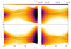Fig. 1. Proper motion of the peaks in the Sgr celestial frame as a function of ${\stackrel{\sim }{\mathrm{\Lambda }}}_{\odot }$. Top: ${\mathrm{\mu }}_{{\stackrel{\sim }{\mathrm{\Lambda }}}_{\odot }}$ coordinate of the kinematic structures detected, weighted by the number of stars in each peak. Bottom: same, but in ${\mathrm{\mu }}_{{\stackrel{\sim }{\beta }}_{\odot }}$. The footprint of the Sgr stream is clearly distinguishable in both the leading and trailing arms. In the latter, we note a sharp edge and a diffuse component above and below it (top and bottom panels, respectively). The lines represent the upper and lower limits of our kinematic selection.

Amidst these two populations, the signal of the Sgr stream appears clearly in what at first sight seems to be a thin kinematic structure. Upon closer inspection, we realised that the trailing arm of the stream (${\stackrel{\sim }{\mathrm{\Lambda }}}_{\odot }<0°$) is better described by a sharp edge, marked by the dash-dotted lines in Fig. 1, and a diffuse envelope (solid black lines). In both ${\mathrm{\mu }}_{{\stackrel{\sim }{\mathrm{\Lambda }}}_{\odot }}$ and ${\mathrm{\mu }}_{{\stackrel{\sim }{\beta }}_{\odot }}$, we observe a decrease in density going from the dash-dotted line to the solid line. To the best of our knowledge, this is the first time we can reach this level of detail with observational data. In the leading arm (${\stackrel{\sim }{\mathrm{\Lambda }}}_{\odot }>0°$) we do not note any substructure, probably due to the fact that this portion of the stream is mostly at larger heliocentric distances. We then adapted the shape proposed by Ibata et al. (2020), and reproduced in Eq. (2) for convenience, to describe the shape of the proper motion trends of the Sgr stream. The result is the eight lines shown in Fig. 1, for which we used the parameters of Table B.1, chosen to produce a visual match to the data². Consequently, we only selected the peaks whose pmra-pmdec coordinates fall inside the contours delineated by said lines:

$$\begin{array}{c}\hfill {\mathrm{\mu }}_X({\stackrel{\sim }{\mathrm{\Lambda }}}_{\odot })=a_1\sin (a_2{\stackrel{\sim }{\mathrm{\Lambda }}}_{\odot }+a_3)+a_4+a_5{\stackrel{\sim }{\mathrm{\Lambda }}}_{\odot }+a_6{{\stackrel{\sim }{\mathrm{\Lambda }}}_{\odot }}^2.\end{array}$$(2)

The resulting selection of peaks for the Sgr stream can be seen in Fig. 2 with the histogram coloured by counts in a Mollweide projection of the sky. It is clear that there is still a significant fraction of contamination from both the thick disc and halo components. This can also be confirmed when looking at the colour-magnitude diagram (CMD) of the stars contributing to each individual peak, since halo and thick disc stars have CMDs clearly distinct from those of the Sgr stream. The most telling factor is the sign of the correlation between colour and apparent magnitude: Sgr presents the typical shape of a red giant branch (negative correlation), whereas the contamination has a triangle shape with a positive correlation (see Fig. B.2).

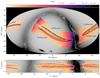Fig. 2. Sky distribution of the candidate Sgr stream stars. Top: mollweide projection of the histogram, in ICRS coordinates, of the counts obtained from the peaks selected in proper motion (Sect. 2.2). The contours are iso-probability lines of Prob(Sgr|${\stackrel{\sim }{\mathrm{\Lambda }}}_{\odot },{\stackrel{\sim }{\beta }}_{\odot }$), a score assigned to each source in the final catalogue based on the probability of being a Sgr stream star (see text). In the background, we included a black and white histogram of the input sample for reference. Bottom: histogram of the stars in our final sample, with bins of 1° × 1°, but in the Sgr reference frame (${\stackrel{\sim }{\mathrm{\Lambda }}}_{\odot }$, ${\stackrel{\sim }{\beta }}_{\odot }$). The red (blue) crosses correspond to the peaks of the 1D WT associated with the bright (faint) branch, while the dashed lines represent the resulting polynomials (see Table 1). The Sgr stream appears as a four-tailed structure across the whole sky, for the first time, in a homogeneous astrometric sample.

We introduce a novel technique to increase the purity of the sample based on the distinct CMD track that each population has. First, we used query 2 in Appendix A to count the number of stars that each peak contains along with four indicators that summarise the main properties of their CMDs: mean colour G_BP − G_RP, mean magnitude G, spread in colour σ_{GBP − GRP} and, finally, the Pearson correlation r_{G − colour}. Then, we applied a simple k-means clustering algorithm to the summary statistics of the CMDs that we obtained for each peak, in combination with their respective average ${\stackrel{\sim }{\mathrm{\Lambda }}}_{\odot }$ and ${\stackrel{\sim }{\beta }}_{\odot }$, after properly normalising the different quantities. We used six components to represent the three main populations present in our data: Sgr, halo and disc. Each of them separate cleanly even with such a simple set-up. This produces a list of peaks candidates that potentially belong to the Sgr stream.

After this last step we obtained the list of candidate substructures, from which we extracted the final sample of 773 612 candidate stars brighter than G  <  19.75 mag, shown in Table C.1 and available at the CDS. Compared to previous samples, this sample is almost three times as big and, in particular, it contains ∼75% of the 294 344 sources in Antoja et al. (2020) and ∼72% of the 263 438 sources in Ibata et al. (2020). While it is tempting to classify all the missing sources in those catalogues as contaminants, it is worth mentioning that, due to some of the steps introduced in our method, the completeness in some regions of the sky is not as high as we would wish. Nonetheless, our sample contains 8060 RR-Lyrae, which is almost exactly the value predicted by Cseresnjes (2001) and right in between the two samples (one pure but incomplete, and one complete but contaminated) given in Ramos et al. (2020).

We complemented our sample with radial velocities obtained from the Apache Point Observatory Galactic Evolution Experiment (APOGEE; Majewski et al. 2017) and the Sloan Extension for Galactic Understanding and Exploration (SEGUE; Yanny et al. 2009), both obtained from the Sloan Digital Sky Survey DR17 (Abdurro’uf et al. 2022), the Large Sky Area Multi-Object Fiber Spectroscopic Telescope (LAMOST DR6; Cui et al. 2012; Zhao et al. 2012), Gaia DR2 (Gaia Collaboration 2018), and SIMBAD (Wenger et al. 2000). We combined all radial velocities (after some minor quality filters; see Appendix B.4) into a single value for each source by taking their median. We did the same for the spectroscopic metallicities (S/Ng-band ≥ 10 for LAMOST, for SEGUE, and SNREV ≥ 20 for APOGEE) but, this time, we did not merge the different catalogues into one value. Instead, we treated each catalogue independently. Finally, we also included reddening-free Wesenheit distances (computed from the Gaia DR2 G band and BP–RP colours) for our sub-sample of RR-Lyrae using the calibration of Neeley et al. 2019.

3. Results

In this section we analyse the changes in each dimension (position, kinematics, and chemistry), and their correlations, along the whole stream.

3.1. Spatial distribution

To better quantify the shape of the branches, we ran a 1D WT on the smoothed ${\stackrel{\sim }{\beta }}_{\odot }$ histograms of the peaks (weighted by counts) every 5° ± 10° in ${\stackrel{\sim }{\mathrm{\Lambda }}}_{\odot }$. From the WT obtained at each bin in ${\stackrel{\sim }{\mathrm{\Lambda }}}_{\odot }$ we extracted the ${\stackrel{\sim }{\beta }}_{\odot }$ values of the peaks. Some of these peaks should correspond to the centre of every over-density present in the ${\stackrel{\sim }{\beta }}_{\odot }$ histograms. And, indeed, we find that the highest ones trace accurately the spine of the bright branch – the main branch– along the whole stream. We also detected a coherent trace of peaks (usually the second or third in height) that follow the over-densities observed by eye and corresponding to the faint branches. Therefore, we assigned each peak accordingly to either the faint or bright branch, from which we obtained four sequences in ${\stackrel{\sim }{\mathrm{\Lambda }}}_{\odot }-{\stackrel{\sim }{\beta }}_{\odot }$ coordinates (two for the leading arm and two for the trailing). Finally, we fitted second-order polynomials of the form ${\stackrel{\sim }{\beta }}_{\odot }({\stackrel{\sim }{\mathrm{\Lambda }}}_{\odot })=a{{\stackrel{\sim }{\mathrm{\Lambda }}}_{\odot }}^2+b{\stackrel{\sim }{\mathrm{\Lambda }}}_{\odot }+c$ to the sky coordinates of each of them, obtaining the coefficients reported in Table 1. The use of the 1D WT requires only the assumption that the peak of the WT coincides with the peak of the density, which we tested with some toy models built from a simple superposition of Gaussians with different means and dispersion. Finally, we compared our results to the ${\stackrel{\sim }{\beta }}_{\odot }$ histograms of the RR Lyrae sub-sample (see Fig. B.3), obtaining a good match that is also compatible with the results of Ramos et al. (2020, leading arm only).

Having obtained a mathematical description of the branches, we would also like to quantify the probability of any star in our sample belonging to any of the four branches of Sgr. To do so, however, we must assume a width along the tails. For simplicity, we chose to model each branch as Gaussians of constant width (i.e. with the same angular size on the sky along the branch). In contrast to the fits of Koposov et al. (2012), we chose smaller widths, σ_Bright = 2.5° and σ_Faint = 1.5°, to describe our data. With this, we obtained a simple way of separating Sgr’s four arms and, also, a way of measuring the probability of any given star in our final sample belonging to the stream based on its sky position with

$$\begin{array}{c}\hfill \begin{array}{c}\hfill \mathrm{Prob}(\mathrm{Sgr}|{\stackrel{\sim }{\mathrm{\Lambda }}}_{\odot },{\stackrel{\sim }{\beta }}_{\odot })=\mathrm{Prob}(\mathrm{A}|{\stackrel{\sim }{\mathrm{\Lambda }}}_{\odot },{\stackrel{\sim }{\beta }}_{\odot })+\mathrm{Prob}(\mathrm{B}|{\stackrel{\sim }{\mathrm{\Lambda }}}_{\odot },{\stackrel{\sim }{\beta }}_{\odot })\\ \hfill -\mathrm{Prob}(\mathrm{A}|{\stackrel{\sim }{\mathrm{\Lambda }}}_{\odot },{\stackrel{\sim }{\beta }}_{\odot })\mathrm{Prob}(\mathrm{B}|{\stackrel{\sim }{\mathrm{\Lambda }}}_{\odot },{\stackrel{\sim }{\beta }}_{\odot }),\end{array}\end{array}$$(3)

where Prob(A|${\stackrel{\sim }{\mathrm{\Lambda }}}_{\odot },{\stackrel{\sim }{\beta }}_{\odot }$) and Prob(B|${\stackrel{\sim }{\mathrm{\Lambda }}}_{\odot },{\stackrel{\sim }{\beta }}_{\odot }$) are the normalised (the mode has a probability of 1) Gaussian probabilities of belonging, respectively, to the bright and faint branches. In Fig. 2 we show the contours delineating three levels of the probability Prob(Sgr|${\stackrel{\sim }{\mathrm{\Lambda }}}_{\odot },{\stackrel{\sim }{\beta }}_{\odot }$) of our final sample (black and white lines). This is the most continuous coverage, obtained from an all-sky astrometric sample of individual stars, of the four arms of the Sgr stream to date.

3.2. Kinematics

Next, we used the mathematical description of each arm to study the kinematics of the stream. After weighting the proper motions and radial velocities with either $\mathrm{Prob}(\mathrm{A}|{\stackrel{\sim }{\mathrm{\Lambda }}}_{\odot },{\stackrel{\sim }{\beta }}_{\odot })$ or $\mathrm{Prob}(\mathrm{B}|{\stackrel{\sim }{\mathrm{\Lambda }}}_{\odot },{\stackrel{\sim }{\beta }}_{\odot }),$ we noted that the differences between the mean trends of the bright and faint branches, despite being larger than 3σ in some portions of the stream, can be easily attributed to projection effects (see Fig. 3). For instance, in the case of the proper motions, we observe a similar trend with ${\stackrel{\sim }{\mathrm{\Lambda }}}_{\odot }$ when comparing the centre of the stream with the stars at the symmetric location of the faint branch with respect to the bright branch. In the case of the radial velocities, there is a smooth transition from positive to negative ${\stackrel{\sim }{\beta }}_{\odot }$, with the physical centre of the stream lying in the middle of the radial velocity track. We also looked at the distances (using both RR Lyrae and the median apparent magnitude) and did not find any evidence of a bi-modality. In other words, we do not observe the existence of two populations in any phase-space dimension other than in the sky position.

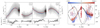Fig. 3. Proper motions and radial velocities of the bright (red) and faint (blue) branches of the Sgr stream. Left: proper motions of the two branches and their differences with 3σ error bars, computed as the standard error of the weighted mean (Cochran 1977). Right: radial velocity coloured by ${\stackrel{\sim }{\beta }}_{\odot }$ for the sources with Prob(ϖ) > 0.8 (see text). The solid (first wrap) and dashed (second and third wraps) correspond to the leading (black) and trailing (grey) arms of the V21 model. Although the differences between the bright and faint branches are significant, they are most likely caused exclusively by the correlation between distance, proper motion, and ${\stackrel{\sim }{\beta }}_{\odot }$.

Figure 3 (right panel) also includes the predictions of the V21 N-body model for the radial velocities as a function of ${\stackrel{\sim }{\mathrm{\Lambda }}}_{\odot }$. As can be seen, our sample contains not only the main branches (solid lines), some halo and thick disc contamination (cloud of points centred around zero radial velocity), but also older wraps as well (dashed and dotted lines). Indeed, our results are consistent with previous 6D samples such as Yang et al. (2019) and Peñarrubia & Petersen (2021). In the latter, the authors report also the detection of old material in the trailing arm. In our sample, this corresponds to the diffuse cloud of points at ${\stackrel{\sim }{\mathrm{\Lambda }}}_{\odot }\sim 100°$. Analogously, we associated the small clump of stars at ${\stackrel{\sim }{\mathrm{\Lambda }}}_{\odot }\sim -100°$ and V_los ∼ 150 km s⁻¹ with the leading arm. While this feature has been associated in the past with Sgr (see e.g. Yang et al. 2019; Peñarrubia & Petersen 2021), and while there is no reason to expect an overdensity at V_los ∼ 150 km s⁻¹ in the radial velocity profile of halos stars in this direction of the sky, we cannot fully rule out that part, or all, of this bump is caused by halo contamination, although it is unlikely given the selections that we made regarding the CMDs. If we do assume that these stars belong to the stream, though, we would be detecting only the older portions of the leading arm at the point where the second and third wraps should cross each other. The use of radial velocities would allow us to, on one hand, obtain a purer selection of 6D stars and, on the other, to constrain the past orbit of Sgr with much better accuracy.

Focusing now on the trailing arm, which we can analyse in greater detail since it is much closer to us than most of the leading, in Fig. 4 we studied the correlations between the proper motions, in particular ${\mathrm{\mu }}_{{\stackrel{\sim }{\mathrm{\Lambda }}}_{\odot }}$, and the distances. For this exercise we did not make any distinction between the bright and faint branches. The advantage of this sample, being so large, is that we can obtain detailed CMDs for each portion of the ${\mathrm{\mu }}_{{\stackrel{\sim }{\mathrm{\Lambda }}}_{\odot }}-{\stackrel{\sim }{\mathrm{\Lambda }}}_{\odot }$ diagram (or ${\mathrm{\mu }}_{{\stackrel{\sim }{\beta }}_{\odot }}-{\stackrel{\sim }{\mathrm{\Lambda }}}_{\odot }$ for that matter) as exemplified by the small histograms surrounding the top panel of Fig. 4. Then, we set out to measure the peak in the apparent magnitude histogram, corresponding to the G magnitude of the red clump, G_RC, and use that as tracer of the distance. To this end, we first fitted a Gaussian kernel to the G histogram of the sources in each bin in ${\stackrel{\sim }{\mathrm{\Lambda }}}_{\odot }$ versus ${\mathrm{\mu }}_{{\stackrel{\sim }{\mathrm{\Lambda }}}_{\odot }}$, from which we then extracted the peaks – using the same code we use for the WT peaks– and sort them by height. The peak of the RC is usually the highest one. In some cases, though, the highest peak corresponded to the magnitude limit imposed (i.e. the histogram diverges towards the faint end due to the presence of the main sequence). When this happened, we simply took the second highest peak. As a result, we coloured each ${\stackrel{\sim }{\mathrm{\Lambda }}}_{\odot }$ versus ${\mathrm{\mu }}_{{\stackrel{\sim }{\mathrm{\Lambda }}}_{\odot }}$ bin by the corresponding G_RC, as can be seen in the top panel of Fig. 4, from which it is obvious that there is a correlation between the modulus of the proper motion vector and the heliocentric distance. This tendency is further confirmed using RR Lyrae distances³, shown in panel a of the same figure.

Fig. 4. Tangential proper motion as a function of ${\stackrel{\sim }{\mathrm{\Lambda }}}_{\odot }$, coloured by different distance estimators, for the trailing arm. Top: coloured by the G magnitude of the red clump, as exemplified by the CMDs surrounding the panel (no extinction correction). Bottom: same projection, now coloured by distance, but for the RR Lyrae in our sample (a) as well as three different N-body simulations ((b) for LM10, (c) for V21, and (d) for P10). We note a clear correlation between the modulus of the proper motion vector and the distance, with small distances corresponding to larger proper motions. The data are, in general, well reproduced by the recently stripped material (light colours). The black lines correspond to the lower limit used in our selection of the peaks (see Table B.1). The V21 is the model that best represents the data. In darker colours, we show the second wrap of the leading arm, and we note that each model predicts a different distribution and region of overlap with the trailing tail.

While this correlation is, to the best of our knowledge, the first time that it has been reported observationally, it is somewhat expected. The physical explanation is simple: stars on the stream sharing the same 3D velocity will have larger proper motions if they are closer to the observer. Similarly, the stars that are farther will pile up into an over-density at small proper motions, thus creating the sharp edge that we parametrised in Table B.1. This limit is set by the outer layer of the stream, that is, its far-side envelope. Therefore, it tells us about the morphology of the stream in configuration space. Obviously, a spread in velocity will also contribute to the spread in proper motion, making any attempt to estimate the morphology of the stream from the spread in proper motion non-trivial. The reason being is, mostly, the fact that the velocity dispersion along the stream is correlated with the thickness of said stream. On the other hand, we note that the V21 model presents a proper motion spread that resembles the data, from which we can extrapolate that the width of the real Sgr stream should be similar to that of the model: ∼20 kpc. In turn, according to the ∼5 kpc dispersion estimated in Hernitschek et al. (2017) for the line-of-sight depth, that would imply that roughly 95% of the Sgr stream stars in the trailing arm should be contained within that ∼20 kpc range.

What is less intuitive, and yet also completely expected, is that the geometry of the Sgr tails, which can be approximated to a cylinder for the following argument, is deformed when observed from the Sun, causing the stream to appear broader on the sky when considering the nearby stars, and more collimated when taking only the stars farther away from us. In other words, as we observed in the V21 model, the stream seems to ‘fan out’ in the sky as the ${\stackrel{\sim }{\beta }}_{\odot }$ distribution of the stellar debris grows broader with decreasing heliocentric distance. It is therefore more likely to have a star closer to us at large values of ${\stackrel{\sim }{\beta }}_{\odot }$, and therefore also at large values of $|{\mathrm{\mu }}_{{\stackrel{\sim }{\mathrm{\Lambda }}}_{\odot }}|$ and $|{\mathrm{\mu }}_{{\stackrel{\sim }{\beta }}_{\odot }}|$.

In this regard, we did not see any evidence of two different populations at high ${\stackrel{\sim }{\beta }}_{\odot }$ neither in proper motion space (which is obvious since we forced a cut in proper motion space) nor in distance⁴ (only one red clump at any given position on the sky). This in turn means that, whatever the nature of the bifurcation is, it must behave very similar to the canonical first wrap of the trailing arm within the range $-120°\lesssim {\stackrel{\sim }{\mathrm{\Lambda }}}_{\odot }\lesssim -50°$.

Panels b–d of Fig. 4 show the same space as (a) but for the stellar particles obtained from three different N-body models created to replicate the Sgr stream. Respectively, these are the LM10, V21 and Peñarrubia et al. (2010, P10) models. The difference between LM10 and P10 is just the internal dynamics of the progenitor as, in case of the latter, Sgr is a rotationally supported system. On the other hand, the main difference between LM10 and V21 is the inclusion of the LMC, which in turn also requires modifying the shape of the MW halo to produce a stream compatible with Sgr. All three models predict a similar first wrap for the trailing arm (in all projections of phase-space), but the V21 model is the one that best reproduces the observations, as can be seen by comparing the lower envelope of their proper motion trends with the lower bound that we obtained from the data (black solid line). The biggest difference between the models, though, is in their ancient stripped material (darker coloured dots), as each model predicts a different trend and site of crossing with the trailing arm. Due to the potentially high constraining power of this old branch, it is very valuable.

3.3. Chemistry

Finally, we analysed the chemical composition of the Sgr stream. To do that, we used the spectroscopic metallicities of APOGEE, LAMOST, and SEGUE. In the top panel of Fig. 5 we show the [α/M] versus [Fe/H] diagram of the stream using APOGEE⁵ (available for 1249 of our candidate sources), where we noted a slight bend in the sequence at a metallicity [Fe/H] ∼ −0.7, which is present throughout the whole stream. The sequence then remains flat until it bends again at [Fe/H] ∼ −0.3. According to the recent work of Hasselquist et al. (2021), who studied in detail the chemical composition of Sgr with 946 APOGEE stars, this is probably the result of a starburst that happened ∼5–7 Gyr ago, followed by a quenching in star formation some ∼3 Gyr ago, both most likely due to the influence of the MW.

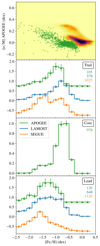Fig. 5. Chemical composition of the Sgr stream. Top panel: [α/M] against [Fe/H] of the stream with APOGEE data (in the background, the same but for the whole APOGEE sample). Bottom panel: Normalised metallicity distribution function for the trailing ($-150°<{\stackrel{\sim }{\mathrm{\Lambda }}}_{\odot }<-40°$), core ($-40°<{\stackrel{\sim }{\mathrm{\Lambda }}}_{\odot }<20°$), and leading ($20°<{\stackrel{\sim }{\mathrm{\Lambda }}}_{\odot }<150°$) parts (top, middle, and bottom, respectively) in bins of 0.2 dex, shifted vertically for clarity. Top right part of each panel we show the number of stars. All three samples, LAMOST, APOGEE, and SEGUE, agree that the leading arm is more metal poor than the trailing.

Below the [α/M] versus [Fe/H] diagram we show, in three separate panels, the metallicity distribution function in the trailing, core and leading parts of the stream, from top to bottom, respectively. All three surveys agree on the fact that the trailing tail is, on average, ∼0.3 dex more metal rich than the leading tails⁶, as noted in previous works (e.g. Yang et al. 2019; Hayes et al. 2020). This is still the case even if we select stars with high Prob(Sgr|${\stackrel{\sim }{\mathrm{\Lambda }}}_{\odot }$,${\stackrel{\sim }{\beta }}_{\odot }$) and high Prob(ϖ)⁷, and even if we refine our kinematic selection by using also the radial velocities shown in Fig. 3. One could argue that this metallicity difference is caused by the fact that the leading arm starts at ${\stackrel{\sim }{\mathrm{\Lambda }}}_{\odot }>40°$, thus corresponding to slightly older material than the trailing arm, but we also checked that the metallicity of the leading arm is systematically lower than the trailing arm at any ${\stackrel{\sim }{\mathrm{\Lambda }}}_{\odot }$. The same applies as a function of Galactic latitude, disfavouring a disc contamination bias. The [α/M] tells the same story given that the leading arm shows a higher mean [α/M] ratio. Moreover, despite the apparently large discrepancy between LAMOST and SEGUE mean metallicity, we find that it is driven by differences in the temperature distribution of the stars within them. Selecting only cold stars in both sub-samples, their mean metallicities agree much better, while preserving the main trends observed in Table 2. Therefore, despite the formal uncertainty floor on the mean metallicity being around 0.14 dex⁸, the metallicity difference of ∼0.3 dex between leading and trailing is robust.

Finally, our results suggest that the faint branch is more metal poor than the bright branch. While all three surveys agree on that, the differences are smaller than the uncertainty floor for APOGEE and LAMOST data, meaning that a re-examination of the chemical properties of the branches with future spectroscopic datasets is in order. Also, the [α/M] for the faint branch seems to be higher than for the bright, in accordance with the [Fe/H]. However, the latter should be treated as a hint rather than a claim since our data are not significant enough on their own. We could not do the same analysis in the trailing arm due to the footprints of the surveys used as there are too few stars on the faint branch. However, Koposov et al. (2012) shows that the faint branch of the trailing arm is also metal poor and probably made of ancient stripped material. Therefore, by association, it seems likely that this is also the case for the faint branch in the leading arm (see also Belokurov et al. 2014). We note, however, that the mean [Fe/H] of the bright branch in the leading arm is still lower than that of the trailing arm. The source of this difference is not clear but it could be due to the fact that in the leading arm there are older wraps of the stream mixed with the young leading arm, as we show in Fig. 3.

4. Discussion

Having studied the properties of our Sgr sample, we now focus on understanding the origin of the bifurcation. For that, we rely on two different models of the stream: V21, which does not exhibit any bifurcation but is an excellent fit to the bright portion of the stream, and P10, which reproduces the bifurcation in the leading arm by modelling the Sgr progenitor as a stellar disc rotating within a Dark matter halo.

In Fig. 6 we show a schematic representation of the V21 model for the Sgr stream. Each colour represents an individual stripping event that the simulated dwarf galaxy has suffered. These correspond to, from bottom to top, the first, second and third pericentre passages, respectively. The gap that exists between the beginning of the first pericentre stripped material and the progenitor (the grey sphere at the top centre) is caused by the quiescent time between the first and second pericentre where almost no material is stripped, and tells us about both the stripping history and orbit of the progenitor. We also include the notation that we use of the different wraps (see caption). For the remainder of the paper we refer to each portion of the stream with the format L1p1h, where the first letter distinguishes between (L)eading and (T)railing, the first number corresponds to the stripping time (first, second, or third pericentre), and the second one expresses the location along the stream (first, second, or third half).

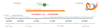Fig. 6. Schematic representation of the stream based on the V21 model. The lines represent the ${\stackrel{\sim }{\mathrm{\Lambda }}}_{\odot }$ extent of the material ejected during each perigalacticon, while their width is proportional to the amount of particles they contain. The blue line is for the stellar particles stripped near the first pericentre, the orange for the second one, and the green for the most recent pericentre passage. We also include the nomenclature of the wraps and the halves into which we divide the stream. As can be seen, the leading arm has stretched more than the trailing, probably due to the shorter dynamical timescale. The 3D distribution in galactocentric coordinates of the stellar particles is shown in the top right inset. Finally, the red arrows represent the range of our data (see Fig. 1), and the hatched portion is where we detect the faint branches of the bifurcation.

– L#p1h ($0°\le {\stackrel{\sim }{\mathrm{\Lambda }}}_{\odot }\le 180°$): First half of the leading arm material stripped at the # pericentre. First wrap.

– L#p2h ($180°\le {\stackrel{\sim }{\mathrm{\Lambda }}}_{\odot }\le 360°$): Second half of the leading arm material stripped at the # pericentre. First wrap.

– L#p3h ($360°\le {\stackrel{\sim }{\mathrm{\Lambda }}}_{\odot }\le 540°$): Third half of the leading arm material stripped at the # pericentre. Second wrap.

– T#p1h ($0°\ge {\stackrel{\sim }{\mathrm{\Lambda }}}_{\odot }\ge -180°$): First half of the trailing arm material stripped at the # pericentre. First wrap.

– T#p2h ($-180°\ge {\stackrel{\sim }{\mathrm{\Lambda }}}_{\odot }\ge -360°$): Second half of the trailing arm material stripped at the # pericentre. First wrap.

– T#p3h ($-360°\ge {\stackrel{\sim }{\mathrm{\Lambda }}}_{\odot }\ge -540°$): Third half of the trailing arm material stripped at the # pericentre. Second wrap.

With this schema in mind, we used Fig. 7 to re-detect the bifurcation in the Sgr data and confirm that the morphology obtained from the 2D analysis of the stream (see Sect. 2.2) is accurate. The left panels of Fig. 7 are obtained after we fold the stream along the line in ${\stackrel{\sim }{\beta }}_{\odot }$ of maximum density (i.e. using the equation in Table 1 for the bright branches) and subtract the stellar count on both sides of the stream. As a result, we obtained the two heat maps for both the trailing (top) and leading (bottom) arms. We note that the amount of stars in the faint branches represent roughly an excess of twice the number of expected stars at that position of the stream. Koposov et al. (2012) quantified, instead, the difference between the bright and faint branches in terms of integrated luminosity, finding that they differ by a factor of 5–10 in the trailing arm.

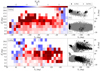Fig. 7. Normalised difference in counts between the two halves of the stream, folded in ${\stackrel{\sim }{\beta }}_{\odot }$ along the line of highest density. The upper script of ${\stackrel{\sim }{\beta }}_{\odot }^f$ stands for ‘folded’. The grey dash lines correspond to the difference between the polynomials of the faint and bright branches (Table 1). On the right, we include ${\stackrel{\sim }{\mathrm{\Lambda }}}_{\odot }$ versus ${\stackrel{\sim }{\beta }}_{\odot }$ scatter plots of the stellar particles in the V21 and P10 N-body models, after applying a similar kinematic filter to the one used for the data, and separating by the time of stripping (black for the first pericentre, grey for the second). The bifurcation in the Sgr stream is obvious in the data and coincides with the functional form fitted in Sect. 2.2. Also, the P10 model presents a clear bimodality, qualitatively similar to the data, produced by the first pericentre material.

We cannot repeat exactly the same exercise with the models due in part to the few particles available, but also because of the differences with the data. Instead, we show the distribution of the stellar particles in the ${\stackrel{\sim }{\mathrm{\Lambda }}}_{\odot }$ versus ${\stackrel{\sim }{\beta }}_{\odot }$ space separating by the pericentre at which they got stripped: the first pericentre (black dots) or the second (grey dots). We selected the particles in proper motion space along the corresponding kinematic tracks, thus mimicking our filter (Table B.1) and allowing for a meaningful comparison with our data. We corroborate that V21 does not produce a bifurcation (the first and second pericentre material are well aligned in the first wrap) while, in contrast, the P10 model does have a bifurcation in both leading and trailing tails, although the latter only extends up to ${\stackrel{\sim }{\mathrm{\Lambda }}}_{\odot }\lesssim -160°$. We note also that, even with the proper motion selection, we still have some leading arm particles crossing the trailing arm at negative ${\stackrel{\sim }{\mathrm{\Lambda }}}_{\odot }$ in both models, which can be seen around ${\stackrel{\sim }{\mathrm{\Lambda }}}_{\odot }\sim -100°$ in V21 and at ${\stackrel{\sim }{\mathrm{\Lambda }}}_{\odot }\sim -120°$, ${\stackrel{\sim }{\mathrm{\Lambda }}}_{\odot }\sim -70°$ in P10.

The utility of the schema presented in Fig. 6 becomes apparent when trying to understand the origin of the bifurcation. As can be seen, exactly at the location of the observed bifurcation in the leading arm there is an overlap between L2p1h and L1p1h. This overlap is almost perfect in 6D phase-space according to the V21 model for the following reason: the particles that were stripped last on the first pericentre did not separate significantly from the progenitor until they approached together the next (second) pericentre. At that moment, the newly stripped material started to spread in the sky in almost the same way as the first pericentre material. Moreover, there is almost an order of magnitude fewer stripped particles at the first pericentre compared to the second pericentre, according to V21. All in all, if this is also the case for the real Sgr stream, it would be really hard to disentangle these two populations from our data with the level of precision we currently have. Indeed, we have been unable to detect two populations in phase-space along the bright branch of the leading arm but the uncertainties are far too large to discard that, within it, there is material from two different pericentres. The only observable that could aid us here would be their chemistry since the L1p should contain particles that were less bound to Sgr (i.e. with smaller initial binding energies) than L2p, and this should correlate with their age and location within the progenitor, which, in turn, should correlate with their [Fe/H] and [α/M]. As can be seen in Table 2, we do find two chemical populations in the leading arm. However, these correspond to the bright (more metal rich) and faint (more metal poor) branches, which we interpret then as the L2p1h and L1p1h, respectively. If that is the case, it means that the L2p1h and L1p1h material got ejected into slightly different orbits, causing a significant misalignment only on the sky distribution. This is easily falsifiable for we should expect a sudden increase in metallicity at the ${\stackrel{\sim }{\mathrm{\Lambda }}}_{\odot }$ before which there is no L1p1h material (${\stackrel{\sim }{\mathrm{\Lambda }}}_{\odot }\lesssim 65°$ in the case of V21). However, the spectroscopic surveys that we use did not provide us with any source in this part of the stream. In the case of APOGEE, which does cover the southern sky, this is due to a lack of fields in this particular direction.

While the P10 model has been shown to not reproduce well the observations (Peñarrubia et al. 2011, and also our Fig. 4), it is a good example of how to produce a bifurcation in the Sgr stream with a disc-like galaxy. Łokas et al. (2010), in particular, showed that it is actually possible to reproduce reasonably well the current properties of the Sgr remnant starting from a galaxy with a rotating disc that, as it falls inside the MW, gets stirred by the tidal field until is no longer recognisable (see also Łokas et al. 2015). Surprisingly enough, the schema of P10 is qualitatively the same as that of V21. However, the inclusion of a dominant rotational component causes three effects: first, it launches the L/T–1p material into a different orbital plane, causing a misalignment between L1p1h and L2p1h at the present day that resembles the observed bifurcation. Secondly, it ejects roughly three times more particles at its first pericentre than in the second pericentre. This point is important because it means that, as expected, the relative brightness of the two branches is sensitive to the internal dynamics of the progenitor. Lastly, the resulting leading bifurcation has as the faint branch the L2p1h, while the L1p1h takes the role of the bright branch. This should cause the bright branch to be more metal poor, in contradiction with our observations. This last point, however, is not a critical issue since the configuration of the stream is sensitive to the relative angle between the angular momentum of the rotating component and the angular momentum of the Sgr orbit, which has never been explored systematically (but see Oria et al. 2022). So, there could in principle exist another configuration where the faint branch is in fact the L1p1h.

The trailing bifurcation is a bit trickier to analyse in this context basically because of the huge gap between the progenitor and the first pericentre material seen in the models (Fig. 6). In other words, neither V21 nor P10 have a substantial T1p1h. Nonetheless, from the sky position of the T1p2h in P10 (see Fig. 7, upper-right panel) one can easily infer that, if it had material deposited along the T1p1h, this would indeed produce a bifurcation. All that is required to populate this part of the stream is that the stripping lasted longer after the first pericentre. The amount of stars that are stripped ‘after’ the pericentre passage depends (among other things) on the ratio between peri- and apocentric distance, which in turn is sensitive to dynamical friction. It is important to recall at this point that V21 does not have a live MW halo and, as a consequence, it relies on the Chandrasekhar description to account for dynamical friction, a recipe known to be inaccurate⁹. Therefore, it could be that by re-doing the simulation in a full N-body fashion, the stream presents a more prominent T1p1h. Another way to modify the stripping history is by altering the initial energy distribution of the stars prior to the first pericentre. This initial distribution function is not trivial to infer from the present-day observations. Nonetheless, the fact that neither V21 nor P10 have a T1p1h could just be a problem of sampling since both have very few particles and, in case of the former, only 4% of the stellar particles are stripped at the first pericentre. We believe this last explanation could not account entirely for the missing component but is a factor to take into account.

Another interesting aspect of models V21 and P10 is that both predict different L1p2h and L1p3h. However, we have only been able to find, unequivocally, first pericentre material at the place where the two parts of the stream cross each other, as can be seen in Fig. 3 (see also Yang et al. 2019 and Peñarrubia & Petersen 2021). This is the location with the least constraining power. We tried actively looking for the rest of the L1p2h and L1p3h, specifically where it intersects the T2p1h, without success. If we were to find these stars they would constrain the whole ancient tail and, thus, allow us to better understand the formation of the bifurcation. We note, however, that the detection of Navarrete et al. (2017, Figs. 5 and 11 in particular) is naturally explained by this T2p1h-L1p2/3h crossing, to the extent that the point of maximum overlap at ${\stackrel{\sim }{\mathrm{\Lambda }}}_{\odot }\sim -70°$ is accurately predicted by V21 model. Incidentally, we have a similar situation in the leading arm with the so called C branch (e.g. Fellhauer et al. 2006), which again is consistent with the crossing of, in this case, the L2p1h and the T1p2h (comparing Table 2 of Correnti et al. 2010, with the V21 model).

There have been other mechanisms proposed in the past to explain the bifurcations, starting with Fellhauer et al. (2006) where they tried to reproduce the faint branch by the overlapping of multiple old and young wraps, displaced relative to one another by the natural orbital precession introduced by the asphericity of the halo. However, their model did not match later observations of the stream. In general, precession alone is probably not enough to reproduce the observations as it requires the faint branch stars to have been ejected before the bright branch. However, to produce such a significant overdensity (see Fig. 7), stars would have had to be ejected after Sgr had lost most of its dark matter shielding, which probably happened at the antepenultimate pericentre. That would naturally lead to models where the faint and bright branches are ejected at consecutive pericentres. Such scenarios would simply be slight modifications on Fellhauer et al. (2006). Moreover, if precession was the cause of the bifurcation one would expect the orbital plane of the faint branch to cross that of the bright branch, forming an X-shape that is not observed.

Law & Majewski (2010), on the other hand, discussed a different possibility: orbital anisotropy within the progenitor, which could be inherent to Sgr or produced by the influence of a Sgr satellite. Both scenarios would modify the distribution of stars in the energy versus angular momentum space and could somewhat mimic the effect of a disc. Naively, though, one would expect the effect on the stream to be milder compared to that of an actual disc. Nonetheless, a detailed prediction is not available in the literature, thus making it difficult to reject these hypothesis at the moment. Koposov et al. (2012) also suggested the idea that the faint branch could actually be the stream of a satellite companion of Sgr. We find this scenario unlikely based on the fact that the CMDs do not show any hint of two distinct populations, despite the faint branch being the dominant component at those ${\stackrel{\sim }{\beta }}_{\odot }$. In this scenario, it would be unexpected for the companion satellite, being less massive than Sgr, to host such a large intermediate age population as the main Sgr stream does since less massive dSph are typically dominated by old and more metal poor stellar populations (e.g. Grebel 2000; Tolstoy et al. 2009). It will be interesting to study other scenarios and test, among other things, whether the trailing branches merge, cross, diverge (in distance with respect to the Sun) or simply stop at Lambda∼ − 40°.

Based on the current data and the discussion presented here, we conclude that the most likely scenario is that the antepenultimate pericentre material and the penultimate pericentre material have been ejected in slightly different orbital planes. Whether this difference comes from the rotation of the progenitor as proposed in P10 or, instead, from an unknown perturbation to the Sgr orbit, is still not clear. The former seems able to produce branches of comparable brightness since it alters the ejection rate at earlier times (compared to a non-rotating progenitor) whereas, in the latter, we might have to tweak the initial energy distribution of the Sgr stars to obtain the correct relative brightness between branches. This shall be the focus of our future studies on the stream.

5. Conclusions

In this work we have exploited the recent Gaia eDR3 astrometric sample to detect the Sgr stream and compile a list of more than 700 000 candidate stars. Thanks to the vast size of the sample obtained and the quality of the Gaia astrometry and photometry, we have been able to characterise the stream in great detail, especially the phase-space distribution of the trailing arm. As a result, we have quantified the correlation between the proper motions and the distance, which allows us to obtain a precise 6D picture of the stream. More importantly, we detect a significant over-density at ${\stackrel{\sim }{\beta }}_{\odot }\ge 5°$ throughout most of the part of the stream that we recognise as the bifurcation. Based on the available data, and thanks to the analysis of tailored N-body models of the stream, we conclude that the most likely origin for this feature is the orbital displacement of the material stripped shortly after the antepenultimate pericentre with respect to the material ejected during the penultimate pericentre.

With this work we have accomplished:

1. An update of our previous Sgr sample, which is now approximately three times larger.

2. A numerical quantification of the sky distribution of the stream and the four branches (the two main ones and the two responsible for the bifurcations).

3. A precise characterisation of the kinematics (together with their correlation with distance) of the whole first wrap of the stream, and even beyond in the case of the radial velocity.

4. The identification and parameterisation of the sharp edge in proper motion space that defines the outermost layer of the stream in 3D space.

5. The chemical properties of the different portions of the stream, showing that the lower metallicity of the leading arm is caused by the overlap with older wraps.

6. A better understanding of the nature of the bifurcation as, according to our interpretation, it is due to the orbital misalignment of the material stripped ≳2 Gyr ago with respect to the material stripped in the penultimate pericentre passage (∼1 Gyr ago).

Looking forwards, we should explore the models of the stream more deeply to find under which circumstances a bifurcation could be formed. Especially challenging is the fact that both faint branches are on the same side of the bright branch, which, in the scenario laid out in this work, would mean that a simple change in the orbital plane of the debris would not be enough as that would most certainly cause an X-shape in the sky. In any case, the streams produced by dwarf galaxies with a rotating component deserve more attention since there has never been a systematic exploration of the angle between the angular momentum of the rotating component and the orbital plane, the properties of said rotating component, or its mass relative to the total mass of the dwarf galaxy, to mention the most relevant free parameters (these topics are addressed in Oria et al. 2022). Nonetheless, either in the case of a rotating progenitor or an external and unknown perturbation, there is scientific value in exploring these scenarios since both have implications for other fields. For instance, if the Sgr orbit is perturbed, we should be able to constrain the properties of said perturber and, perhaps, also its impact on the stellar distribution of the MW itself (if any).

To aid us in constraining the models, we should (i) obtain more observations of the stream, focusing on the chemical properties of the faint branches, especially for the trailing arm, (ii) locate the ancient wraps in other, more informative, places of the sky, and (iii) statistically test if the differences in kinematics between bright and faint branches are explained by projection effects (and differential solar reflex) alone or not, which requires a rigorous treatment of said effects. By doing so, we could produce more accurate fits and better understand the interaction between Sgr, the MW, and the Magellanic Clouds.

Acknowledgments

We would like the thank the referee for their deep and constructive comments and suggestions. We thank Raphaël Errani and Simon Rozier for all their useful comments. This work has made use of data from the European Space Agency (ESA) mission Gaia (https://www.cosmos.esa.int/gaia), processed by the Gaia Data Processing and Analysis Consortium (DPAC, https://www.cosmos.esa.int/web/gaia/dpac/consortium). Funding for the DPAC has been provided by national institutions, in particular the institutions participating in the Gaia Multilateral Agreement. This work has been supported by the Agence Nationale de la Recherche (ANR project SEGAL ANR-19-CE31-0017). It has also received funding from the project ANR-18-CE31-0006 and from the European Research Council (ERC grant agreement No. 834148). TA acknowledges the grant RYC2018-025968-I funded by MCIN/AEI/10.13039/501100011033 and by “ESF Investing in your future”. This work was (partially) funded by the Spanish MICIN/AEI/10.13039/501100011033 and by “ERDF A way of making Europe” by the “European Union” through grant RTI2018-095076-B-C21, and the Institute of Cosmos Sciences University of Barcelona (ICCUB, Unidad de Excelencia “María de Maeztu”) through grant CEX2019-000918-M. This project has received support from the DGAPA/UNAM PAPIIT program grant IG100319. Z.Y. acknowledges support from the French National Research Agency (ANR) funded project “Pristine” (ANR-18-CE31-0017). Guoshoujing Telescope (the Large Sky Area Multi-Object Fiber Spectroscopic Telescope LAMOST) is a National Major Scientific Project built by the Chinese Academy of Sciences. Funding for the project has been provided by the National Development and Reform Commission. LAMOST is operated and managed by the National Astronomical Observatories, Chinese Academy of Sciences. This research has made use of the SIMBAD database, operated at CDS, Strasbourg, France. Funding for the Sloan Digital Sky Survey IV has been provided by the Alfred P. Sloan Foundation, the U.S. Department of Energy Office of Science, and the Participating Institutions. SDSS-IV acknowledges support and resources from the Center for High Performance Computing at the University of Utah. The SDSS website is www.sdss.org. SDSS-IV is managed by the Astrophysical Research Consortium for the Participating Institutions of the SDSS Collaboration including the Brazilian Participation Group, the Carnegie Institution for Science, Carnegie Mellon University, Center for Astrophysics | Harvard & Smithsonian, the Chilean Participation Group, the French Participation Group, Instituto de Astrofísica de Canarias, The Johns Hopkins University, Kavli Institute for the Physics and Mathematics of the Universe (IPMU)/University of Tokyo, the Korean Participation Group, Lawrence Berkeley National Laboratory, Leibniz Institut für Astrophysik Potsdam (AIP), Max-Planck-Institut für Astronomie (MPIA Heidelberg), Max-Planck-Institut für Astrophysik (MPA Garching), Max-Planck-Institut für Extraterrestrische Physik (MPE), National Astronomical Observatories of China, New Mexico State University, New York University, University of Notre Dame, Observatário Nacional/MCTI, The Ohio State University, Pennsylvania State University, Shanghai Astronomical Observatory, United Kingdom Participation Group, Universidad Nacional Autónoma de México, University of Arizona, University of Colorado Boulder, University of Oxford, University of Portsmouth, University of Utah, University of Virginia, University of Washington, University of Wisconsin, Vanderbilt University, and Yale University.

References

Appendix A: Queries to the Gaia archive

The results presented in this work have been obtained using the following queries to the Gaia Archive:

Listing 1. Query to obtain the proper motion histogram at a certain HEALpix.

SELECT COUNT(*) as N, pmra_index*BINSIZE as pmra,
     pmdec_index*BINSIZE as pmdec FROM (SELECT
     gaia.source_id, FLOOR(pmra/BINSIZE) AS
     pmra_index, FLOOR(pmdec/BINSIZE) AS pmdec_index,
     agn.catalogue_name FROM gaiaedr3.gaia_source AS
     gaia LEFT OUTER JOIN gaiaedr3.agn_cross_id AS
     agn ON agn.source_id = gaia.source_id WHERE
     gaia.source_id BETWEEN HPNUM*2**35*4**(12-LVL)
     AND (HPNUM+1)*2**35*4**(12-LVL) AND
     parallax_over_error BETWEEN -PLXCUT AND PLXCUT)
     AS sub WHERE sub.catalogue_name IS NULL GROUP BY
     pmra_index, pmdec_index

where HPNUM is the number of the HEALpix tile being processed, LVL is the level of the HEALpix tessellation (here, 6), BINSIZE is the binning of the histogram in proper motion (0.12 mas yr⁻¹), and finally, PLXCUT is the maximum parallax quality allowed (see Eq. 1).

Listing 2. Query to obtain the main characteristics of the CMD for the stars in a peak in proper motion space.

SELECT count(*) as N, ((SUM(phot_g_mean_mag *
    bp_rp)-(SUM(phot_g_mean_mag) * SUM(bp_rp)) /
    COUNT(*)))/(SQRT(SUM(phot_g_mean_mag *
    phot_g_mean_mag)-(SUM(phot_g_mean_mag)*SUM
    (phot_g_mean_mag)) / COUNT(*))*SQRT(SUM(bp_rp *
    bp_rp)-(SUM(bp_rp) * SUM(bp_rp)) / COUNT(*))) AS
    r, avg(phot_g_mean_mag) as g, avg(bp_rp) as
    colour,
    SQRT((COUNT(*)/(COUNT(*)-1))*(avg(POWER(bp_rp,2))
    - POWER(avg(bp_rp),2))) as std_colour, avg(ra)
    as ra, avg(dec) as dec, avg(pmra) as pmra,
    avg(pmdec) as pmdec FROM gaiaedr3.gaia_source AS
    gaia LEFT OUTER JOIN gaiaedr3.agn_cross_id AS
    agn ON agn.source_id = gaia.source_id WHERE
    gaia.phot_g_mean_mag < maxG and gaia.g_rp is not
    Null AND gaia.source_id BETWEEN
    HPNUM*2**35*4**(12-LVL) AND
    (HPNUM+1)*2**35*4**(12-LVL) AND
    parallax_over_error BETWEEN -PLXCUT AND PLXCUT
    AND agn.catalogue_name IS NULL AND
    (POWER((gaia.pmra-PEAK_PMRA),2)+
    POWER((gaia.pmdec-PEAK_PMRA),2)) <
    (2*PEAK_RADIUS)**2

from which we obtain the main photometric properties (mean, dispersion and Pearson’s correlation coefficient) of an over-density in proper motion space. To do so, on one hand we limit the faintest magnitude allowed maxG (19.75 mag in this work). On the other, we use the three parameters that defined any peak: PEAK_PMRA, PEAK_PMDEC, and PEAK_PMRADIUS.

Appendix B: Details of the methodology

B.1. Proper motion analysis

Each proper motion histogram obtained at each HEALpix is transformed with the WT (Starck & Murtagh 2002) to enhance and isolate the significant over-densities in kinematic space, which are then selected with the peak_local_max algorithm included in the Python package Scikit-image (van der Walt et al. 2014). The result at each HEALpix is a list of peaks for each scale of the WT characterised by a centre (pmra-pmdec coordinates) a radius, r = binsize  ×  2^scale, and its WT coefficient defined by

$$\begin{array}{c}\hfill I(x,y)=c_N(x,y)+{\displaystyle \sum _{j=0}^{N-1}{\omega }_j(x,y),}\end{array}$$(B.1)

where I is the input histogram, c_N is its smoothed version, and ω_j are the arrays of WT coefficients at each of the N scales j ∈ [0, N − 1].

Of course, any real structure will appear as an over-density at several (if not all) of the WT scales in which the original histogram is decomposed. However, in our previous works (Antoja et al. 2020; Ramos et al. 2021) we chose, for simplicity, to select only the most prominent peak throughout all scales, one per HEALpix. To be able to deal with all the information returned by the WT, we define the following two concepts.

Kinematic trees We considered all peaks in all scales, and we used a method to organise them into unique structures that we name ‘kinematic trees’. It goes as follows (see Fig. B.1 for reference): for each HEALpix, we began with a peak at scale 0 (the smallest layer), which we call p_i, and then took all the peaks at scale 1, p_i + 1, that fall within the circular area defined by p_i (r_i = binsize  ×  2ⁱ). We did not restrict ourselves to a single peak at the scale i + 1 and, as such, allowed these ‘trees’ to ‘branch out’. For each of the peaks found at scale 1, we repeated the process but at scale 2. The process continued until we reached the largest scale, at which point we moved to the next 0-scale peak and started over again. Once we did this for every peak in our sample across all HEALpix, we ended up with a set of hierarchical structures that are characterised by the pmra-pmdec coordinates of the peak with the highest ω_j, which in turns also sets the characteristic size of the whole structure, r_j. Each of these kinematic trees now represent a unique kinematic structure.

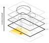Fig. B.1. Schematic representation of the WT and the kinematic trees. From a proper motion histogram (bottommost plane), a series of layers (numbered as in Eq. B.1) are extracted, each with a number of peaks. These peaks may be caused by the same structure and can be linked into isolated kinematic trees (see text).

Absorbing Poisson noise We still have the problem that Poisson noise can create several small-scale peaks at the same HEALpix for a single object. In that case, they will quickly merge at the upper scales once the size of the peaks can absorb the noise. We correct for this ‘duplicity’ by merging the trees that share the same scale-1 peak¹⁰ (r = 0.24 mas yr⁻¹). In practice, this is very similar as starting from histograms with a coarser binning, but not exactly.

Parameters of the kinematic selection In Table B.1 we show the parameters used to isolate the kinematic signature of the Sgr stream (see Sect. 2.2).

K-means clustering After selecting the peaks based on the proper motion trends of the Sgr stream, we obtained the photometric summary statistics of each of them using query 2. We then ran a k-means clustering with six clusters on the vector (${\stackrel{\sim }{\mathrm{\Lambda }}}_{\odot }$, ${\stackrel{\sim }{\beta }}_{\odot }$, r_{G − colour}, < G> , < G_{BP − RP}> , σ_{GBP − RP}), which we re-normalised so that all quantities have a comparable range.

The results can be seen in Fig. B.2, where we show all peaks in the space of r_{G − colour} against σ_{GBP − RP}, highlighting those tagged as Sgr stream (dark contours). Surrounding the main panel, we included examples of the CMDs that the peaks contain depending on their photometric properties, showing that the K-means clustering has indeed separated the different populations correctly.

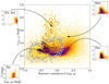Fig. B.2. Result of the K-means clustering. Centre: Histogram in the space of rG − colour versus σGBP − RP weighted by the number of stars of the peaks that fulfil the filter of Table B.1. The contours correspond to the peaks labelled Sgr stream. Bottom left: Example of a CMD obtained from the peaks associated with Sgr. Bottom right: Same but peaks associated with the disc. Top right: Same but for the halo. Top left: Same but for the very extincted disc.

B.2. The RR Lyrae sub-sample

In our list of candidate Sgr stars we find 8084 RR Lyrae, of which 8066 have a period-Wesenheit distances (based solely on Gaia photometry). Their sky distribution is shown in Fig. B.3 where it can be seen to follow closely the polynomials of Table 1.

Fig. B.3. Similar to bottom panel of Fig. 2 but showing the RR Lyrae sub-sample (black dots).

B.3. Using parallax_over_error to discern contamination

When looking at the CMDs of our final sample at different position along the stream, we noticed a persistent source of contamination that does not follow any isochrone shape. Upon further inspection, we see that these correspond to either halo or thick disc stars (depending on the region on the sky). Luckily, the parallax_over_error distribution of these contaminant sources does not follow the same distribution as the Sgr stars. In fact, the non-Sgr stars tend to have larger values of parallax_over_error, thus deforming an otherwise symmetric Gaussian distribution. We took advantage of this by: (1) finding the mode of the distribution, (2) mirroring only the part of the histogram left to said mode (the negative side), (3) stitching together the original negative side with its mirrored version, and (4) fitting a normal distribution to it.

This results in a symmetric probability distribution of parallax_over_error that describes accurately the Sgr stream (μ = 0.29 mas, σ = 1.12 mas). In reality, one would have to do this at ‘every’ position in the sky both because of the distance gradient and because the parallax zero point is position dependent (Lindegren et al. 2021). In practice, the Sgr coordinates are almost aligned with the ICRS frame, causing the stream to do only small excursions in ecliptic latitude and, as a consequence, the variations on the zero point are very small. On the other hand, the distance gradient is almost negligible once inverted into parallaxes, especially because the progenitor contains many more stars than the tidal tails.

Finally, we normalised the p.d.f. and assigned a probability to each star based on how close the observed distribution is to the expected number. In other words, the stars that lie close to the mode will get a score close to 1, while those lying in a region where there is a lot of contamination will get a low score. We call this score Prob(ϖ).

B.4. Adding radial velocities

The radial velocities used in this work have been compiled from five different catalogues: APOGEE, LAMOST, SEGUE, Gaia DR2 and SIMBAD. Each catalogue has its own caveats but we decided to simplify the merging by computing the median radial velocities with just the measurements that pass the following filters:

• APOGEE: signal to noise larger than 10,

• LAMOST: error in velocity smaller than 20 km s⁻¹,

• SEGUE: based on the recommendations described in their web page, we used the cut (sp.zwarning = 0 OR sp.zwarning = 16) AND sp.elodiervfinalerr != 0 AND sp.snr > 35,

• Gaia: no cut,

• SIMBAD: no cut.

Appendix C: Sagittarius eDR3 sample

In Table C.1 we show ten stars of our final sample of the Sgr stream, which can be found online at the CDS website. The description of the columns can be seen in the caption of the table.

All Tables

All Figures

Fig. 1. Proper motion of the peaks in the Sgr celestial frame as a function of ${\stackrel{\sim }{\mathrm{\Lambda }}}_{\odot }$. Top: ${\mathrm{\mu }}_{{\stackrel{\sim }{\mathrm{\Lambda }}}_{\odot }}$ coordinate of the kinematic structures detected, weighted by the number of stars in each peak. Bottom: same, but in ${\mathrm{\mu }}_{{\stackrel{\sim }{\beta }}_{\odot }}$. The footprint of the Sgr stream is clearly distinguishable in both the leading and trailing arms. In the latter, we note a sharp edge and a diffuse component above and below it (top and bottom panels, respectively). The lines represent the upper and lower limits of our kinematic selection.

In the text

Fig. 2. Sky distribution of the candidate Sgr stream stars. Top: mollweide projection of the histogram, in ICRS coordinates, of the counts obtained from the peaks selected in proper motion (Sect. 2.2). The contours are iso-probability lines of Prob(Sgr|${\stackrel{\sim }{\mathrm{\Lambda }}}_{\odot },{\stackrel{\sim }{\beta }}_{\odot }$), a score assigned to each source in the final catalogue based on the probability of being a Sgr stream star (see text). In the background, we included a black and white histogram of the input sample for reference. Bottom: histogram of the stars in our final sample, with bins of 1° × 1°, but in the Sgr reference frame (${\stackrel{\sim }{\mathrm{\Lambda }}}_{\odot }$, ${\stackrel{\sim }{\beta }}_{\odot }$). The red (blue) crosses correspond to the peaks of the 1D WT associated with the bright (faint) branch, while the dashed lines represent the resulting polynomials (see Table 1). The Sgr stream appears as a four-tailed structure across the whole sky, for the first time, in a homogeneous astrometric sample.

In the text

Fig. 3. Proper motions and radial velocities of the bright (red) and faint (blue) branches of the Sgr stream. Left: proper motions of the two branches and their differences with 3σ error bars, computed as the standard error of the weighted mean (Cochran 1977). Right: radial velocity coloured by ${\stackrel{\sim }{\beta }}_{\odot }$ for the sources with Prob(ϖ) > 0.8 (see text). The solid (first wrap) and dashed (second and third wraps) correspond to the leading (black) and trailing (grey) arms of the V21 model. Although the differences between the bright and faint branches are significant, they are most likely caused exclusively by the correlation between distance, proper motion, and ${\stackrel{\sim }{\beta }}_{\odot }$.

In the text

Fig. 4. Tangential proper motion as a function of ${\stackrel{\sim }{\mathrm{\Lambda }}}_{\odot }$, coloured by different distance estimators, for the trailing arm. Top: coloured by the G magnitude of the red clump, as exemplified by the CMDs surrounding the panel (no extinction correction). Bottom: same projection, now coloured by distance, but for the RR Lyrae in our sample (a) as well as three different N-body simulations ((b) for LM10, (c) for V21, and (d) for P10). We note a clear correlation between the modulus of the proper motion vector and the distance, with small distances corresponding to larger proper motions. The data are, in general, well reproduced by the recently stripped material (light colours). The black lines correspond to the lower limit used in our selection of the peaks (see Table B.1). The V21 is the model that best represents the data. In darker colours, we show the second wrap of the leading arm, and we note that each model predicts a different distribution and region of overlap with the trailing tail.

In the text

Fig. 5. Chemical composition of the Sgr stream. Top panel: [α/M] against [Fe/H] of the stream with APOGEE data (in the background, the same but for the whole APOGEE sample). Bottom panel: Normalised metallicity distribution function for the trailing ($-150°<{\stackrel{\sim }{\mathrm{\Lambda }}}_{\odot }<-40°$), core ($-40°<{\stackrel{\sim }{\mathrm{\Lambda }}}_{\odot }<20°$), and leading ($20°<{\stackrel{\sim }{\mathrm{\Lambda }}}_{\odot }<150°$) parts (top, middle, and bottom, respectively) in bins of 0.2 dex, shifted vertically for clarity. Top right part of each panel we show the number of stars. All three samples, LAMOST, APOGEE, and SEGUE, agree that the leading arm is more metal poor than the trailing.

In the text

Fig. 6. Schematic representation of the stream based on the V21 model. The lines represent the ${\stackrel{\sim }{\mathrm{\Lambda }}}_{\odot }$ extent of the material ejected during each perigalacticon, while their width is proportional to the amount of particles they contain. The blue line is for the stellar particles stripped near the first pericentre, the orange for the second one, and the green for the most recent pericentre passage. We also include the nomenclature of the wraps and the halves into which we divide the stream. As can be seen, the leading arm has stretched more than the trailing, probably due to the shorter dynamical timescale. The 3D distribution in galactocentric coordinates of the stellar particles is shown in the top right inset. Finally, the red arrows represent the range of our data (see Fig. 1), and the hatched portion is where we detect the faint branches of the bifurcation.

In the text

Fig. 7. Normalised difference in counts between the two halves of the stream, folded in ${\stackrel{\sim }{\beta }}_{\odot }$ along the line of highest density. The upper script of ${\stackrel{\sim }{\beta }}_{\odot }^f$ stands for ‘folded’. The grey dash lines correspond to the difference between the polynomials of the faint and bright branches (Table 1). On the right, we include ${\stackrel{\sim }{\mathrm{\Lambda }}}_{\odot }$ versus ${\stackrel{\sim }{\beta }}_{\odot }$ scatter plots of the stellar particles in the V21 and P10 N-body models, after applying a similar kinematic filter to the one used for the data, and separating by the time of stripping (black for the first pericentre, grey for the second). The bifurcation in the Sgr stream is obvious in the data and coincides with the functional form fitted in Sect. 2.2. Also, the P10 model presents a clear bimodality, qualitatively similar to the data, produced by the first pericentre material.

In the text

	Fig. B.1. Schematic representation of the WT and the kinematic trees. From a proper motion histogram (bottommost plane), a series of layers (numbered as in Eq. B.1) are extracted, each with a number of peaks. These peaks may be caused by the same structure and can be linked into isolated kinematic trees (see text).
In the text

Fig. B.2. Result of the K-means clustering. Centre: Histogram in the space of rG − colour versus σGBP − RP weighted by the number of stars of the peaks that fulfil the filter of Table B.1. The contours correspond to the peaks labelled Sgr stream. Bottom left: Example of a CMD obtained from the peaks associated with Sgr. Bottom right: Same but peaks associated with the disc. Top right: Same but for the halo. Top left: Same but for the very extincted disc.

In the text

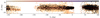	Fig. B.3. Similar to bottom panel of Fig. 2 but showing the RR Lyrae sub-sample (black dots).
In the text

References

- Abdurro’uf, Accetta, K., Aerts, C., et al. 2022, ApJS, 259, 35 [NASA ADS] [CrossRef] [Google Scholar]
- Alard, C. 1996, ApJ, 458, L17 [NASA ADS] [Google Scholar]
- Antoja, T., Ramos, P., Mateu, C., et al. 2020, A&A, 635, L3 [NASA ADS] [CrossRef] [EDP Sciences] [Google Scholar]
- Belokurov, V., Zucker, D. B., Evans, N. W., et al. 2006, ApJ, 642, L137 [Google Scholar]
- Belokurov, V., Koposov, S. E., Evans, N. W., et al. 2014, MNRAS, 437, 116 [NASA ADS] [CrossRef] [Google Scholar]
- Cochran, W. G. 1977, Sampling Techniques, 3rd edn. (John Wiley) [Google Scholar]
- Correnti, M., Bellazzini, M., Ibata, R. A., Ferraro, F. R., & Varghese, A. 2010, ApJ, 721, 329 [Google Scholar]
- Cseresnjes, P. 2001, A&A, 375, 909 [NASA ADS] [CrossRef] [EDP Sciences] [Google Scholar]
- Cui, X.-Q., Zhao, Y.-H., Chu, Y.-Q., et al. 2012, Res. Astron. Astrophys., 12, 1197 [Google Scholar]
- de Boer, T. J. L., Belokurov, V., Beers, T. C., & Lee, Y. S. 2014, MNRAS, 443, 658 [NASA ADS] [CrossRef] [Google Scholar]
- Dierickx, M. I. P., & Loeb, A. 2017, ApJ, 836, 92 [NASA ADS] [CrossRef] [Google Scholar]
- Everall, A., & Boubert, D. 2022, MNRAS, 509, 6205 [Google Scholar]
- Fahlman, G. G., Mandushev, G., Richer, H. B., Thompson, I. B., & Sivaramakrishnan, A. 1996, ApJ, 459, L65 [NASA ADS] [Google Scholar]
- Fardal, M. A., van der Marel, R. P., Law, D. R., et al. 2019, MNRAS, 483, 4724 [NASA ADS] [CrossRef] [Google Scholar]
- Fellhauer, M., Belokurov, V., Evans, N. W., et al. 2006, ApJ, 651, 167 [NASA ADS] [CrossRef] [Google Scholar]
- Gaia Collaboration (Prusti, T., et al.) 2016, A&A, 595, A1 [NASA ADS] [CrossRef] [EDP Sciences] [Google Scholar]
- Gaia Collaboration (Brown, A. G. A., et al.) 2018, A&A, 616, A1 [NASA ADS] [CrossRef] [EDP Sciences] [Google Scholar]
- Gaia Collaboration (Brown, A. G. A., et al.) 2021a, A&A, 649, A1 [NASA ADS] [CrossRef] [EDP Sciences] [Google Scholar]
- Gaia Collaboration (Antoja, T., et al.) 2021b, A&A, 649, A8 [EDP Sciences] [Google Scholar]
- Gibbons, S. L. J., Belokurov, V., & Evans, N. W. 2014, MNRAS, 445, 3788 [NASA ADS] [CrossRef] [Google Scholar]
- Grebel, E. K. 2000, in Star Formation from the Small to the Large Scale, eds. F. Favata, A. Kaas, & A. Wilson, ESA Spec. Publ., 445, 87 [NASA ADS] [Google Scholar]
- Hasselquist, S., Hayes, C. R., Lian, J., et al. 2021, ApJ, 923, 172 [NASA ADS] [CrossRef] [Google Scholar]
- Hayes, C. R., Majewski, S. R., Hasselquist, S., et al. 2020, ApJ, 889, 63 [Google Scholar]
- Helmi, A. 2004, ApJ, 610, L97 [NASA ADS] [CrossRef] [Google Scholar]
- Hernitschek, N., Sesar, B., Rix, H.-W., et al. 2017, ApJ, 850, 96 [NASA ADS] [CrossRef] [Google Scholar]
- Ibata, R., Irwin, M., Lewis, G. F., & Stolte, A. 2001, ApJ, 547, L133 [Google Scholar]
- Ibata, R., Bellazzini, M., Thomas, G., et al. 2020, ApJ, 891, L19 [NASA ADS] [CrossRef] [Google Scholar]
- Ibata, R. A., Gilmore, G., & Irwin, M. J. 1994, Nature, 370, 194 [Google Scholar]
- Ibata, R. A., Gilmore, G., & Irwin, M. J. 1995, MNRAS, 277, 781 [NASA ADS] [CrossRef] [Google Scholar]
- Ibata, R. A., Wyse, R. F. G., Gilmore, G., Irwin, M. J., & Suntzeff, N. B. 1997, AJ, 113, 634 [Google Scholar]
- Johnston, K. V., Spergel, D. N., & Hernquist, L. 1995, ApJ, 451, 598 [NASA ADS] [CrossRef] [Google Scholar]
- Johnston, K. V., Law, D. R., & Majewski, S. R. 2005, ApJ, 619, 800 [Google Scholar]
- Koposov, S. E., Belokurov, V., Evans, N. W., et al. 2012, ApJ, 750, 80 [NASA ADS] [CrossRef] [Google Scholar]
- Law, D. R., & Majewski, S. R. 2010, ApJ, 714, 229 [Google Scholar]
- Layden, A. C., & Sarajedini, A. 2000, AJ, 119, 1760 [NASA ADS] [CrossRef] [Google Scholar]
- Lindegren, L., Klioner, S. A., Hernández, J., et al. 2021, A&A, 649, A2 [EDP Sciences] [Google Scholar]
- Łokas, E. L., Kazantzidis, S., Majewski, S. R., et al. 2010, ApJ, 725, 1516 [CrossRef] [Google Scholar]
- Łokas, E. L., Semczuk, M., Gajda, G., & D’Onghia, E. 2015, ApJ, 810, 100 [CrossRef] [Google Scholar]
- Majewski, S. R., Skrutskie, M. F., Weinberg, M. D., & Ostheimer, J. C. 2003, ApJ, 599, 1082 [NASA ADS] [CrossRef] [Google Scholar]
- Majewski, S. R., Schiavon, R. P., Frinchaboy, P. M., et al. 2017, AJ, 154, 94 [NASA ADS] [CrossRef] [Google Scholar]
- Martínez-Delgado, D., Aparicio, A., Gómez-Flechoso, M. Á., & Carrera, R. 2001, ApJ, 549, L199 [CrossRef] [Google Scholar]
- Mateo, M., Mirabal, N., Udalski, A., et al. 1996, ApJ, 458, L13 [Google Scholar]
- Mateo, M., Olszewski, E. W., & Morrison, H. L. 1998, ApJ, 508, L55 [NASA ADS] [CrossRef] [Google Scholar]
- Navarrete, C., Belokurov, V., Koposov, S. E., et al. 2017, MNRAS, 467, 1329 [NASA ADS] [Google Scholar]
- Neeley, J. R., Marengo, M., Freedman, W. L., et al. 2019, MNRAS, 490, 4254 [Google Scholar]
- Oria, P.-A., Ibata, R., Ramos, P., Famaey, B., & Errani, R. 2022, ApJ, 932, L14 [NASA ADS] [CrossRef] [Google Scholar]
- Peñarrubia, J., & Petersen, M. S. 2021, MNRAS, 508, L26 [CrossRef] [Google Scholar]
- Peñarrubia, J., Belokurov, V., Evans, N. W., et al. 2010, MNRAS, 408, L26 [NASA ADS] [Google Scholar]
- Peñarrubia, J., Zucker, D. B., Irwin, M. J., et al. 2011, ApJ, 727, L2 [CrossRef] [Google Scholar]
- Ramos, P., Mateu, C., Antoja, T., et al. 2020, A&A, 638, A104 [EDP Sciences] [Google Scholar]
- Ramos, P., Antoja, T., Mateu, C., et al. 2021, A&A, 646, A99 [EDP Sciences] [Google Scholar]
- Rybizki, J., Green, G. M., Rix, H.-W., et al. 2022, MNRAS, 510, 2597 [NASA ADS] [CrossRef] [Google Scholar]
- Sarajedini, A., & Layden, A. C. 1995, AJ, 109, 1086 [Google Scholar]
- Shao, S., Cautun, M., Deason, A., & Frenk, C. S. 2021, MNRAS, 504, 6033 [CrossRef] [Google Scholar]
- Siegel, M. H., Dotter, A., Majewski, S. R., et al. 2007, ApJ, 667, L57 [NASA ADS] [CrossRef] [Google Scholar]
- Slater, C. T., Bell, E. F., Schlafly, E. F., et al. 2013, ApJ, 762, 6 [NASA ADS] [CrossRef] [Google Scholar]
- Starck, J.-L., & Murtagh, F. 2002, Astronomical Image and Data Analysis (Springer) [Google Scholar]
- Tepper-García, T., & Bland-Hawthorn, J. 2018, MNRAS, 478, 5263 [CrossRef] [Google Scholar]
- Tolstoy, E., Hill, V., & Tosi, M. 2009, ARA&A, 47, 371 [Google Scholar]
- van der Walt, S., Schönberger, J. L., Nunez-Iglesias, J., et al. 2014, PeerJ, 2, e453 [Google Scholar]
- Vasiliev, E., Belokurov, V., & Erkal, D. 2021, MNRAS, 501, 2279 [NASA ADS] [CrossRef] [Google Scholar]
- Velazquez, H., & White, S. D. M. 1995, MNRAS, 275, L23 [NASA ADS] [Google Scholar]
- Wenger, M., Ochsenbein, F., Egret, D., et al. 2000, A&AS, 143, 9 [NASA ADS] [CrossRef] [EDP Sciences] [Google Scholar]
- Yang, C., Xue, X.-X., Li, J., et al. 2019, ApJ, 886, 154 [NASA ADS] [CrossRef] [Google Scholar]
- Yanny, B., Rockosi, C., Newberg, H. J., et al. 2009, AJ, 137, 4377 [Google Scholar]
- Zhao, G., Zhao, Y.-H., Chu, Y.-Q., Jing, Y.-P., & Deng, L.-C. 2012, Res. Astron. Astrophys., 12, 723 [NASA ADS] [CrossRef] [Google Scholar]