| Issue |
A&A
Volume 666, October 2022
|
|
|---|---|---|
| Article Number | A56 | |
| Number of page(s) | 19 | |
| Section | Extragalactic astronomy | |
| DOI | https://doi.org/10.1051/0004-6361/202142553 | |
| Published online | 06 October 2022 | |
Metal content of the circumgalactic medium around star-forming galaxies at z ∼ 2.6 as revealed by the VIMOS Ultra-Deep Survey
1
Insituto de Física y Astronomía, Universidad de Valparaíso, Avda. Gran Bretaña 1111, 2340000 Valparaíso, Chile
e-mail: This email address is being protected from spambots. You need JavaScript enabled to view it.
2
Dipartimento di Fisica e Astronomia Galileo Galilei, Università degli Studi di Padova, Vicolo del L’Osservatorio 3, 35122 Padova, Italy
3
INAF Osservatorio Astronomico di Padova, Vicolo dell’Osservatorio 5, 35122 Padova, Italy
4
Instituto de Investigación Multidisciplinar en Ciencia y Tecnología, Universidad de La Serena, Raúl Bitrán, 1305 La Serena, Chile
5
Departamento de Astronomía, Universidad de La Serena, Av. Juan Cisternas 1200 Norte, La Serena, Chile
6
Núcleo de Astronomía, Facultad de Ingeniería y Ciencias, Universidad Diego Portales, Av. Ejército 441, Santiago, Chile
7
INAF – Osservatorio di Astrofisica e Scienza dello Spazio di Bologna, Via Gobetti 93/3, 40129 Bologna, Italy
8
INAF-IASF, Via Bassini 15, 20133 Milano, Italy
9
Department of Astronomy, University of Massachusetts Amherst, 710 N. Pleasant St, Amherst, MA 01003, USA
10
Departamento de Ciencias Fisicas, Facultad de Ciencias Exactas, Universidad Andres Bello, Fernandez Concha 700, Las Condes, Santiago, Chile
11
Space Telescope Science Institute, 3700 San Martin Drive, Baltimore, MD 21218, USA
12
Aix Marseille Univ., CNRS, CNES, LAM, Marseille, France
13
Gemini Observatory, NSF’s NOIRLab, 670 N. A’ohoku Place, Hilo, HI 96720, USA
14
Department of Physics and Astronomy, University of California, Davis, One Shields Ave., Davis, CA 95616, USA
15
Instituto de Física, Pontificia Universidad Católica de Valparaíso, Casilla, 4059 Valparaíso, Chile
16
European Southern Observatory, Av. Alonso de Córdova 3107, Vitacura, Santiago, Chile
Received:
30
October
2021
Accepted:
10
June
2022
Abstract
Context. The circumgalactic medium (CGM) is the location where the interplay between large-scale outflows and accretion onto galaxies occurs. Metals in different ionization states flowing between the circumgalactic and intergalactic mediums are affected by large galactic outflows and low-ionization state inflowing gas. Observational studies on their spatial distribution and their relation with galaxy properties may provide important constraints on models of galaxy formation and evolution.
Aims. The main goal of this paper is to provide new insights into the spatial distribution of the circumgalactic of star-forming galaxies at 1.5 < z < 4.5 (⟨z⟩∼2.6) in the peak epoch of cosmic star formation activity in the Universe. We also look for possible correlations between the strength of the low- and high-ionization absorption features (LIS and HIS) and stellar mass, star formation rate, effective radius, and azimuthal angle ϕ that defines the location of the absorbing gas relative to the galaxy disc plane.
Methods. The CGM has been primarily detected via the absorption features that it produces on the continuum spectrum of bright background sources. We selected a sample of 238 close pairs from the VIMOS Ultra Deep Survey to examine the spatial distribution of the gas located around star-forming galaxies and generate composite spectra by co-adding spectra of background galaxies that provide different sight-lines across the CGM of star-forming galaxies.
Results. We detect LIS (C II and Si II) and HIS (Si IV, C IV) up to separations ⟨b⟩ = 172 kpc and 146 kpc. Beyond this separation, we do not detect any significant signal of CGM absorption in the background composite spectra. Our Lyα, LIS, and HIS rest-frame equivalent width (W0) radial profiles are at the upper envelope of the W0 measurements at lower redshifts, suggesting a potential redshift evolution for the CGM gas content producing these absorptions. We find a correlation between C II and C IV with star formation rate and stellar mass, as well as trends with galaxy size estimated by the effective radius and azimuthal angle. Galaxies with high star formation rate (log[SFR/(M⊙ yr−1)] > 1.5) and stellar mass (log[M⋆/M⊙] > 10.2) show stronger C IV absorptions compared with those low SFR (log[SFR/(M⊙ yr−1)] < 0.9) and low stellar mass (log[M⋆/M⊙] < 9.26). The latter population instead shows stronger C II absorption than their more massive or more star-forming counterparts. We compute the C II/C IVW0 line ratio that confirms the C II and C IV correlations with impact parameter, stellar mass, and star formation rate. We do not find any correlation with ϕ in agreement with other high-redshift studies and in contradiction to what is observed at low redshift where large-scale outflows along the minor axis forming bipolar outflows are detected.
Conclusions. We find that the stronger C IV line absorptions in the outer regions of these star-forming galaxies could be explained by stronger outflows in galaxies with higher star formation rates and stellar masses that are capable of projecting the ionized gas up to large distances and/or by stronger UV ionizing radiation in these galaxies that is able to ionize the gas even at large distances. On the other hand, low-mass galaxies show stronger C II absorptions, suggesting larger reservoirs of cold gas that could be explained by a softer radiation field unable to ionize high-ionization state lines or by the galactic fountain scenario where metal-rich gas ejected from previous star formation episodes falls back to the galaxy. These large reservoirs of cold neutral gas around low-mass galaxies could be funnelled into the galaxies and eventually provide the necessary fuel to sustain star formation activity.
Key words: Galaxy: evolution / galaxies: high-redshift / galaxies: star formation
© H. Méndez-Hernández et al. 2022
 Open Access article, published by EDP Sciences, under the terms of the Creative Commons Attribution License (https://creativecommons.org/licenses/by/4.0), which permits unrestricted use, distribution, and reproduction in any medium, provided the original work is properly cited.
This article is published in open access under the Subscribe-to-Open model. This email address is being protected from spambots. You need JavaScript enabled to view it. to support open access publication.
1. Introduction
The circumgalactic medium (CGM, 10 kpc – ∼300 kpc) is the gas reservoir between the interstellar medium (ISM, ≲10 kpc) and the intergalactic medium (IGM, ≳300 kpc). It is characterized as an active interface where galaxies reprocess their baryonic material. Up to ∼50% of the total baryonic mass is found in the CGM at low redshift (z ∼ 0.2; Wolfe et al. 2005; Werk et al. 2014; Zheng et al. 2015) and at high redshift (Hafen et al. 2019), thus representing a significant gas reservoir that can, for example, feed the ISM with gas to form new stars (Zhu & Ménard 2013; Thom et al. 2012; Richter et al. 2016). Supernovae explosions or strong stellar winds can deposit metals in the surrounding medium, gas that is mixed with pristine gas accreted from the IGM (Prochaska & Wolfe 2009; Bauermeister et al. 2010; Tumlinson et al. 2011, 2017; Kacprzak 2017).
Since the first discoveries of circumgalactic gas around star-forming galaxies (Boksenberg & Sargent 1978; Kunth & Bergeron 1984; Bergeron 1986), its study by direct detection of emission has been a challenge (van de Voort & Schaye 2013; Burchett et al. 2021). The CGM has been primarily detected via the absorption features that it produces on light from background sources. In a pioneering study at high redshift (z ≳ 1.5), Adelberger et al. (2003, 2005) studied the dependence of the absorption strength on the projected angular separation between foreground and background galaxies (i.e. impact parameter b); they reported absorption detection at impact parameters up to 40 kpc and found that absorption strength weakens significantly at larger separations. Thanks to their brightness, quasars are typically used as background sources to probe the CGM around foreground galaxies (Bergeron & Boissé 1991; Steidel et al. 1994; Kacprzak et al. 2010), which allows the signal produced by extremely low column densities (NHI ≃ 1012 cm−2) to be identified independently of the properties of the targeted galaxy (e.g. luminosity and/or redshift; Tumlinson et al. 2017; Péroux & Howk 2020). This technique has been used successfully to probe the CGM of galaxies up to redshifts z ∼ 5 (Matejek & Simcoe 2012) and has led to the discovery that the CGM is gas rich and has a multi-phase nature (Adelberger et al. 2003; Steidel et al. 1994; Steidel 1995; Songaila 2001; Tripp et al. 1998; Kacprzak et al. 2010; Werk et al. 2016).
The CGM has been also characterized using the ‘down-the-barrel technique’, which uses the targeted galaxy itself as a background source. Absorption lines redshifted with respect to the galaxy rest-frame give evidence of the presence of gas flowing towards the galaxy. This result has been interpreted as a strong indication of inflowing material onto the host galaxy (Sato et al. 2009; Rubin et al. 2012; Martin et al. 2012), while outflows have been identified as blueshifted absorptions in galaxy spectra (Martin 2005; Chen et al. 2010). Although the location of the gas producing the detected absorption is unconstrained, this technique has been successful in studying galactic inflows and outflows from the spectroscopy of star-forming galaxies up to z ∼ 2 − 3 (Kornei et al. 2012; Rudie et al. 2012; Heckman et al. 2015; Heckman & Borthakur 2016).
Recently, three more techniques have been used to explore the CGM. The first, gravitational-arc tomography, takes advantage of strong gravitational lensing and uses giant bright lensed arcs as background sources to map the CGM of foreground galaxies providing a tomographic view of the absorbing gas (Lopez et al. 2018, 2020; Claeyssens et al. 2019; Tejos et al. 2021; Mortensen et al. 2021). The second technique takes advantage of deep three-dimensional datacubes observations to study the cold CGM of high-redshift (z > 2) star-forming galaxies, and has reported the ubiquitous presence of Lyα haloes in these galaxies (Steidel et al. 2011; Matsuda et al. 2012; Momose et al. 2014; Wisotzki et al. 2016; Leclercq et al. 2017; Chen et al. 2020), whose line properties are correlated to their spatial location (Leclercq et al. 2020) and that can extend up to 4 Mpc beyond the CGM (Chen et al. 2020; Bacon et al. 2021). The third technique uses the spectra of bright afterglows of long gamma-ray bursts (GRBs) to derive the kinematic properties of the CGM gas around their host galaxies and constrain the physical properties (Gatkine et al. 2019, 2022).
Alongside these diverse techniques used to study the CGM, the large spectroscopic extragalactic surveys have allowed the statistical extraction and analysis of the weak signals from different metal absorption using the stacking of hundreds of spectra (Steidel et al. 2010). These large datasets have been helpful to overcome the limitations of finding galaxy–QSOs pairs at concordant redshifts (Steidel et al. 1994; Bouché et al. 2007), increasing statistics, and facilitating vast parameter space exploration (York et al. 2006; Bordoloi et al. 2011; Zhu & Ménard 2013). At low redshift (zmed ∼ 0.5) CGM analyses have been focused on the study of absorption lines of Lyα (Chen et al. 2001a), C IV (Chen et al. 2001b), O VI (Tumlinson et al. 2011), and Mg II (Bowen et al. 1995; Bouché et al. 2007; Steidel et al. 1994), and their dependence on stellar mass (Bordoloi et al. 2011), inclination (Kacprzak et al. 2010), and azimuthal angle (Shen et al. 2012; Bordoloi et al. 2014a). At higher redshifts, the observed metal absorption lines are mostly limited to Si II, C II, C IV, and Si IV; the first two are called low-ionization state (LIS, T = 104 − 4.5 K) lines, and the last two high-ionization state (HIS, T = 104.5 − 5.5 K) lines (Steidel et al. 2010). At high redshift (z > 2) several authors have reported the presence of high-velocity outflows. Lehner et al. (2014) demonstrated that O VI successfully probes outflows in star-forming galaxies, and reported velocity widths in the range 200−400 km s−1. Next, Du et al. (2016) analysed several ionization lines (e.g. Si II, Fe II, Al II, Ni II, Al III, C IV) to probe the multi-phase nature of the CGM and detected C IV blueshifted offsets concordant with 76 km s−1 velocity outflows. Their results show a direct link between C IV absorption and star formation rate. Later on, Jones et al. (2018) reported velocity outflows of ∼150 km−1, as shown by several LIS and HIS absorptions in nine gravitationally lensed star-forming galaxies (z ≃ 2 − 3), suggesting that galaxy outflows regulate the galaxy chemical evolution. Similar outflow detections inferred from different ionization absorption lines have been reported, and stellar mass and star formation rate have been invoked as their main drivers (Zhu & Ménard 2013; Turner et al. 2014; Trainor et al. 2015; Gatkine et al. 2019; Price et al. 2020). However, as suggested by Dutta et al. (2021), LIS and HIS absorption detections (from which velocity outflows can be inferred), could be affected by large-scale environmental processes (Dutta et al. 2021; Wang et al. 2022) or their available neutral gas content (Berry et al. 2012; Oyarzún et al. 2016; Du et al. 2018), and their correlation with stellar mass and star formation rate might in fact be a consequence of a main-sequence offset rather than simply correlated with the star formation rate or stellar mass (Cicone et al. 2016; Gatkine et al. 2022).
Numerical simulations consider that the CGM comes from gas accreted from the IGM, followed by stellar winds from the central galaxy and the gas ejected or stripped from satellites (Hafen et al. 2019; Christensen et al. 2018). Simulations reveal that the accretion efficiency depends on the galaxy stellar mass, decreasing from ∼80% for M⋆ ∼ 106 M⊙ galaxies to ∼60% for M⋆ ∼ 1010 M⊙ galaxies (Dekel et al. 2005; Kereš et al. 2005; Hafen et al. 2020). Once accreted, this material can remain in the CGM for billions of years leading to a well-mixed halo gas before it interacts with the ejected large-scale stellar winds produced by starbursts (Martin 2005; Weiner et al. 2009). At z = 2 most metals are found to be located in the ISM or stars of the central galaxy, and by z = 0.25 most of it will end up in the CGM and IGM (e.g. Peeples et al. 2014; Anglés-Alcázar et al. 2017; Hafen et al. 2020; Oppenheimer et al. 2016; Nelson et al. 2021).
The way in which this pristine material is accreted into galaxies may depend on its location relative to the galaxy disc plane defined by the azimuthal angle (ϕ). Various observational studies highlight a correlation between the strength of the Mg II LIS absorption line and the azimuthal angle (Bordoloi et al. 2011, 2014a; Kacprzak et al. 2011; Bouché et al. 2012, 2013). Although weak Mg II detections along the minor axis have been reported (e.g. Lan et al. 2014), it has been found that strong Mg II absorptions are preferably detected along the major-axis of galaxies, suggesting the presence of inflowing material potentially feeding future star formation. On the other hand, C IV and O VI (HIS lines) absorptions seem stronger along the minor axis, probably evidence of strong stellar winds enriching the CGM (Tumlinson et al. 2011; Kacprzak et al. 2015). Recently, Péroux et al. (2020) used cosmological hydrodynamical simulations to examine the physical properties of the gas located in the CGM of star-forming galaxies (z < 1) as a function of angular orientation. They found that the CGM properties vary strongly with the impact parameter, stellar mass, and redshift. They reported a higher average CGM metallicity at large impact parameters (b > 100 kpc) along the minor versus major axes. Moreover, they tentatively found that the average metallicity of the CGM depends on the azimuthal angle, showing that the low-metallicity gas preferably inflows along the galaxy major axis, while outflows are commonly located along the minor axis, in agreement with previous observations (Bordoloi et al. 2011; Bouché et al. 2012; Kacprzak et al. 2012, 2015). These results present a picture where star-forming galaxies accrete co-planar gas within narrow stream-flows providing fresh fuel for the new generation of stars; later, this population will produce metal-enriched galactic-scale outflows along the minor axis (Kacprzak 2017). However, even though the presence of bipolar outflows collimated along the minor axis is expected to evolve with redshift (expected to be ubiquitous at z = 1), it has been difficult to demonstrate its presence at z = 2, mostly as the result of the absence of gaseous galactic discs sculpting the outflows (Nelson et al. 2019).
In order to better understand the mechanisms of galaxy growth in earlier phases of the history of the Universe, and to investigate a possible cosmic evolution of such mechanisms, similar studies at higher redshifts are needed. Observations along different lines of sight (l.o.s.) can probe different parts of the CGM, and the identification of low- and high-ionization metal absorption lines can give information on the possible multi-phase nature of the CGM. However, using QSO–galaxy pairs to study the CGM is not straightforward as the identification of the galaxies responsible for the metal absorptions detected on the spectra of background quasars is not an easy task. Stacking analyses of background galaxy spectra that are located in the vicinity of foreground galaxies provides an alternative tool to overcome sensitivity limitations, exploiting large extra-galactic surveys containing a large number of individual spectra. In this work we seek to characterize the presence of low- (LIS: O I + Si II, C II, Si II, Fe II), intermediate- (IIS: Al III), and high-ionization (HIS: Si IV, C IV) state metal absorption (see Table 1) in the CGM of a star-forming galaxy population at ⟨z⟩∼2.6 using UV spectra obtained from the large VIMOS Ultra Deep Survey (VUDS; Le Fèvre et al. 2015). We use thousands of galaxies with the most reliable redshift measurements and the highest S/N spectra (with reliability flags 3 and 4; see Le Fèvre et al. 2015; Tasca et al. 2017), a sample broadly representative of the bulk of the star-forming galaxy population at these redshifts (Lemaux et al. 2022). To detect the dim signal coming from low- and high-ionization line absorptions produced in the CGM of these star-forming galaxies, we stack the spectra of close (in projection) background galaxies to establish the metal distribution in the CGM and explore their dependence on the physical and morphological properties of star-forming galaxies (e.g. impact parameter b, star formation rate, stellar mass, galaxy effective radius, and azimuthal angle) at the peak epoch of cosmic star formation activity in the Universe.
Main spectral features observed in our VUDS stacked spectra in the 1100−2000 Å rest-frame range.
The manuscript is organized as follows. Section 2 summarizes the VUDS survey properties relevant to our analyses. Section 3 presents our stacking analysis method for measuring the metal equivalent widths (W0), while Sect. 4 presents our W0 results for Lyα, and multiple LIS, IIS, and HIS metal lines observed our star-forming galaxy sample across different physical and morphological properties. We discuss our results in Sect. 5, and finally we present our conclusions in Sect. 6. Throughout the text we use ΛCDM cosmology with H0 = 70 km s−1 Mpc−1, ΩM = 0.3, and ΩΛ = 0.7, and distances are given in physical units (kpc).
2. The VUDS parent sample
The VUDS has obtained spectra of 5590 galaxies in the redshift range 1.5 < z < 4.5. A detailed description of the survey observations, the methods applied to process the data, and the derived parameters including the spectroscopic redshifts zspec is given in Le Fèvre et al. (2015). A description of the VUDS-DR1 first data release can be found in Tasca et al. (2017). The VUDS spectroscopic targets are selected based on their photometric redshifts and observed optical flux; the targets have zphot + 1σz ≥ 2.4 and iAB ≤ 25. The wavelength range of each spectrum is between 3600 < λ/Å < 9350, accumulating 14 h of integration time in each of the LRBLUE and LRRED grisms of the VIMOS spectrograph on the ESO Very Large Telescope (Le Fèvre et al. 2003), with a spectral resolution R ∼ 230 (∼7 Å) and reaching a S/N = 5 on the continuum at 8500 Å. We note that the VUDS observations were taken using the VIMOS low-resolution multi-slit mode with a minimum slit length optimized to 6 arcsec, maximizing the number of observed slits per mask (see Bottini et al. 2005).
Standard data processing was performed using the VIPGI environment (Scodeggio et al. 2005), followed by redshift measurements using the EZ package (Garilli et al. 2010). The final UV rest-frame flux-limited sample is broadly representative of the bulk of the star-forming galaxy population at these redshifts (2 < z < 5; Lemaux et al. 2022). A critical aspect of VUDS is the large comoving volume covered, totalling 1 deg2 in three fields: COSMOS (Scoville et al. 2007), ECDFS (Giacconi et al. 2002), and VVDS02h (Le Fèvre et al. 2005, 2013).
For the purposes of this study the instrumental set-up translates into the ability to follow lines redder than Lyα (≥ 1215.6 Å) at redshifts higher than 1.5. We decided to restrict the VUDS sample to 2100 galaxies, selected in the redshift range 1.5 < z < 4.5 (zflag = 3, 4, i.e. 95 − 100% probability of being correct). We note that the velocity accuracy of redshift measurements is expected to be in the range dz/(1 + z) = 0.0005 − 0.0007, or an absolute velocity ( ) accuracy 150−200 km (Le Fèvre et al. 2013, 2015; Tasca et al. 2017). The rich broad-band imaging available for galaxies in VUDS is used for spectral energy distribution (SED) fitting (Tasca et al. 2015; Thomas et al. 2017) using the Galaxy Observed-Simulated SED Interactive Program (GOSSIP; Franzetti et al. 2008) to derive various global galaxy properties, for example stellar mass, star formation rate (SFR), dust extinction E(B − V), age, and metallicity.
GOSSIP is a tool that performs SED fitting by using a combination of spectro-photometric measurements from different bands to match a set of synthetic galaxy spectra based on emission from stellar populations. GOSSIP uses model spectra from galaxy population synthesis models (Bruzual & Charlot 2003; Maraston 2005) and uses the probability distribution function (PDF) of each galaxy parameter to determine the best SED fit. Figure 1 shows SFR versus stellar mass for 5590 star-forming galaxies at z > 1.5 and 2 < z < 3.5 selected from the VUDS survey, and the 238 star-forming galaxies that we finally selected and scrutinized in this work (see Sect. 3). These 238 galaxies have stellar masses and star formation rates of log[M⋆/M⊙]) = 9.73 ± 0.4 and log[SFR/(M⊙ yr−1)] = 1.38 ± 0.39.
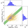 |
Fig. 1. Star formation rate versus stellar mass for 5590 star-forming galaxies selected from the VUDS survey at z > 1.5 (grey open squares) and at 2 < z < 3.5 (yellow crosses), and the 238 star-forming galaxies (blue stars) considered in this work. The black dot-dashed line shows the main sequence of star-forming galaxies for 1.5 < z < 2.5 including its ±.3 dex scatter represented by the green shaded region, as defined by Hathi et al. (2016). Top and right panels: report the distributions in stellar mass and SFR for the 238 star-forming galaxies evaluated in this work. |
Exploiting the Hubble Space Telescope (HST) F814W images (Koekemoer et al. 2007) that are available as part of the COSMOS Survey (Scoville et al. 2007), morphological parameters have been estimated for 1242 star-forming galaxies (zflag = 4, 3, 2, 9, i.e. 75% probability of being correct) with 9.5 < log[M⋆/M⊙] < 11.5. In particular, Ribeiro et al. (2016) run GALFIT (Peng et al. 2002, 2010), a standard parametric profile-fitting tool, estimating Sersic indices (n), azimuthal angles, major-to-minor axis ratios (q), and effective radii (reff). Figure 2 shows the distribution of the 97 selected galaxy pairs (see Sect. 3) with available morphological parameters. Table 2 shows the detailed number of subsets of galaxies.
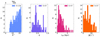 |
Fig. 2. Projected angular separation (θ) amongst galaxy foreground–background galaxy pairs, axial ratio (q), effective radius (reff), and azimuthal angle (ϕ) distributions of the star-forming (foreground) galaxies used in our analyses. The morphological parameters were obtained from the parametric measures of Ribeiro et al. (2016), see Sect. 2 for details. |
VUDS fg–bg galaxy pair sample.
3. Analysis
In this work we describe our probe of the CGM around galaxies at z ∼ 2.6, near the epoch at which the cosmic SFR density of the Universe reaches its peak, by using the spectra of background (bg) galaxies as ‘spotlights’ illuminating the CGM. At these redshifts individual bg galaxies are not bright enough to individually detect low- and high-ionization state metal absorption lines. Thus, we stack spectra of bg galaxies to look for absorption lines produced by the CGM around foreground (fg) star-forming galaxies. To select a sample of close galaxy pairs (fg–bg) out of the VUDS survey, we imposed similar criteria to those described by Steidel et al. (2010): (i) galaxy spectra for the fg and bg galaxies must possess an accurately determined redshift (95 − 100%; see Le Fèvre et al. 2015; Tasca et al. 2017 for details), (ii) a redshift separation 0.1 < zbg − zfg ≤ 1.0 between fg–bg galaxy pairs to ensure that each spectrum contains a significant common spectral coverage after shifting to the rest-frame of the fg galaxy and to avoid an overlap between the fg CGM and the bg galaxy absorptions, and (iii) a maximum projected angular separation of 23″.
Stacking the fg spectra provides the absorptions at the foreground galaxy’s rest-frame. Figure 3 shows the redshift distributions of the foreground and background galaxy pairs and the fg–bg pairs redshift difference (Δz = zbg − zfg) distribution in the top right corner. The spectroscopic sample includes 238 spectra within the redshift range 1.5 < z ≲ 4.43 (⟨z⟩ = 2.6 ± 0.41) and is limited to a 23″ maximum projected angular separation distance amongst galaxy pairs that correspond to 187.2 kpc at z = 2.6. This sample is then split into four different bins according to the angular projected separation,  ,
,  ,
,  , and 20″ < θ ≤ 23″, identified as samples S1, S2, S3, and S4, and were defined in such a way that each bin contains approximately the same number of galaxies (see Table 3) providing a comparable S/N for each composite spectra. These angular projected separation bins correspond to projected physical distances (hereafter impact parameters) b: ≤68.6 kpc, 68.6 kpc < b ≤ 113.5 kpc, 113.5 kpc < b ≤ 146.2 kpc, and 146.2 kpc < b ≤ 172.8 kpc for samples S1, S2, S3, and S4. We note that the conversion from angular separation to physical impact parameter varies ±3% over the full redshift range (1.5 < z < 4.5) of the foreground galaxy sample, thus in the following impact parameter b and projected angular separation θ will be used interchangeably. Table 3 contains a summary of the statistical properties of the galaxy pair samples.
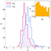 |
Fig. 3. Redshift distribution of the star-forming galaxy pairs (foreground and background) selected in this work. The Δz = zbg − zfg distribution is also included in the top right corner. |
Foreground–background (fg–bg) galaxy pair statistics according to the projected angular separation (θ).
To generate our fg and bg composite spectra we co-added individual spectra as follows. For each pair of galaxies, the spectrum of the fg was (i) shifted to its own rest-frame; (ii) continuum-normalized using the full wavelength range1; (iii) resampled2 to a common wavelength resolution Δλ, defined by the maximum of the shifted wavelength resolution (Δλshf_fg) distribution of the galaxy sample used to generate the composite spectra (e.g. Δλ ∼ 2 Å for fg composite spectra as shown in Fig. 4); and (iv) smoothed with a Gaussian kernel whose width size Δλ was defined before.
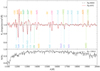 |
Fig. 4. Composite UV spectra of 238 VUDS star-forming galaxies. Top: median (black) and average (red) composite spectra shifted to rest-frame of 238 foreground galaxies with projected angular separations < 23″ (b < 187.2 kpc at z = 2.6). Bottom: fraction of contributing individual spectra to the composite spectra per unit wavelength. Several spectral lines of interest are indicated: H I (Lyα) emission–absorption (blue), low-ionization state metal absorption lines (cyan), intermediate-ionization state metal absorption lines (peach), high-ionization state metal absorption lines (magenta), interstellar fine-structure emission line (green), absorption stellar photospheric lines (gold), emission nebular lines (lime), and emission–absorption lines associated with stellar winds (indigo). |
A similar approach was used to produce stacked spectra of the bg galaxies. Each individual bg galaxy spectrum was (i) shifted into the fg galaxy’s rest-frame using the same systemic redshift applied to their corresponding fg galaxy spectrum; (ii) continuum normalized using the full wavelength range1; (iii) resampled to a common wavelength resolution Δλ, defined by the maximum of the shifted wavelength resolution(Δλshf_bg) distribution of the galaxy sample used to generate the composite spectra; (iv) smoothed with Δλ Gaussian kernel as defined before. The strong interstellar absorption features (see Fig. 4 and Table 1) located at the redshift of each bg rest-frame were masked because they can potentially contaminate the composite signal at the fg rest-frame.
Finally, the foreground and background spectra were co-added independently to produce composite stacked spectra. In all cases, for each spectral bin, we calculated both the average and the median value, eventually producing both an average and median co-added spectrum.
4. Results
Rest-frame UV spectra of star-forming galaxies at redshift z ∼ 3 are commonly dominated by the emission of O and B stars; the CGM and/or IGM media imprint absorption features on this UV continuum (Sargent et al. 1980; Bergeron 1986; Bergeron & Boissé 1991; Lanzetta et al. 1995). Composite spectra can provide different l.o.s. of the average absorption strength produced by the gas located in these media (Adelberger et al. 2005; Shapley et al. 2003). Figure 4 shows the median and average composite spectra by stacking the 238 foreground galaxies. The lower panel shows a histogram of the fraction of galaxies contributing to each spectral bin of the co-added spectrum. In our analysis the separation zero (b = 0) l.o.s. defines the interstellar medium properties of the foreground galaxies, while larger separations (b > 0) l.o.s. define the properties of the CGM around the foreground galaxies at different separations.
While the l.o.s that we use to study the CGM cross through the whole CGM at a given separation, the information about the ISM comes only from the absorptions produced by the gas located in the half-galaxy that is the closest to the observer. For this reason, to compare the strength of the absorptions at separation 0 (the ISM) and at separation > 0 (the CGM), the former need to be corrected for this incompleteness. Following Steidel et al. (2010), we apply the following factors: 1.45 for low-ionization species (Si II, C II), 1.70 for Si IV, and ∼2 for C IV. The different l.o.s. probed by the background galaxy’s light passing through the foreground CGM help us to trace neutral and ionized gas in H II star-forming regions and the large-scale stellar winds produced by star formation activity (Shapley et al. 2003). The main spectral features identified in our fg composite spectra (Fig. 4) in the 1100−2000 Å range are summarized in Table 1.
In the 900−1900 Å range we explored the following absorption lines: Lyα (λ1215.7 Å), O I + Si II (λλ1303.2 Å), C II (λ1334.5 Å), Si IV (λλ1393, 1402 Å), Si II (λ1526.7 Å), C IV (λλ1548.2, 1550.8 Å), Fe II (λ1608.5 Å), Al II (λ1670.8 Å), and Al III (λ1862.8 Å). First, we present their equivalent widths as a function of the angular separation between galaxy pairs (θ) (see Sect. 4.1). We then examine the correlations between the strength of the Lyα, LIS (C II, Si II), and HIS (C IV, Si IV) lines as a function of different galaxy properties, including stellar mass, star formation rate (see Sect. 4.2), effective radius (reff), and the azimuthal angle (ϕ) (see Sect. 4.3). We also explore the C II/C IV line ratio (see Sect. 4.4) as a function of the projected angular separation, stellar mass, and star formation rate.
4.1. Radial dependence
Here we present absorption lines produced by gas located in the CGM of star-forming galaxies at z ∼ 2.6. Figure 5 shows the average absorption spectra obtained after stacking the background galaxy spectra at the redshift of the foreground galaxy as a function of their projected angular separation:  ,
,  –
– ,
,  –20″, and 20″–23″. We note that as a consequence of the VUDS design and selection criteria, the number of galaxies with small projected angular separations (< 6″) is scarce. The strengths of the line absorptions were measured by fitting a single Gaussian profile to the stacked spectra. Equivalent widths (W0) of each line profile are obtained by integrating the Gaussian fit of each stacked spectrum around the central wavelength of the Gaussian fit to the line using an integration window within the ±5σ range.
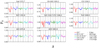 |
Fig. 5. Median absorption lines (thin lines) detected from our 238 foreground–background galaxy pairs, including all foreground galaxies (red) and background galaxies split by their projected angular separations: < 11 |


All equivalent width measurements are given in the rest-frame and we use positive (negative) equivalent widths to indicate absorption (emission). The errors on the equivalent width measurements are determined using a bootstrap approach. For each set of galaxy background spectra, a thousand co-added spectra are generated from random selections, with replacements from that same sample in order to preserve the number of evaluated sources. For each of these co-adds, the line absorption equivalent widths are estimated. The 16th and 84th percentiles of the distribution of equivalent widths are taken as error intervals for the original measurement. We note that owing to the nature of star-forming galaxies, which show a diversity of spectral features (e.g. ISM absorption lines, photospheric stellar and nebular lines, and Lyα emission), the absorption lines in our composite spectra show both an emission and absorption component. The emission components can be produced by the same transition responsible for producing the absorption line (e.g. Lyα), produced by nearby fine-structure transitions, or in some cases they can be completely absent.
Figure 6 shows the radial profiles of the absorption rest-frame equivalent width obtained from the average (red) and median (blue) stacked absorption specrta presented in Fig. 5. Median composite spectra are expected to be free of artefacts and contamination such as sky residuals, unexpected absorption or emission features in the background galaxy spectra. On the other hand, the average composite spectra could be affected by strong absorption lines coming from individual l.o.s. Median and average composite spectra are in general concordant, and trace similar trends. We also tested other combination techniques, including straight average, average sigma-clipping, and average continuum-weighting, which produce very similar composite spectra. Table 4 contains a summary of the measured equivalent widths as a function of the projected angular separation, including the significance (in terms of S/N) of the detections. Noise estimations were computed with the DER_SNR3 algorithm (Stoehr et al. 2008) on a continuum band-pass adjacent to each central absorption line. We limit our analyses to detections with S/N ≥ 3; however, upper limits with S/N < 3 are also included (highlighted using solid black symbols and arrows in Fig. 6) as these detections are useful to outline the possible correlations and/or trends of the profiles. We note that some precautions should be taken when interpreting the absorption strengths of these spectral features as they might not reflect the true conditions of the cold and hot gas CGM components. For instance, the balances amongst singly ionized species of some elements (e.g. Al, Cl) can be altered by dielectronic recombination (Black & Dalgarno 1973; Watson 1973; Jura 1974) or ion-molecule reactions (charge exchange reactions of ionized species with neutral hydrogen and helium Steigman 1975). While the abundances relative to neutral hydrogen of some elements (e.g. O, N, P, Cl, Si, Cr, Mn, Fe, Ni) can be affected by factors of 2−10, Al is depleted by a factor of ∼100 (York & Kinahan 1979), making Al II a biased tracer of the neutral gas phase. In addition, Fe II is contaminated by Fe IV (λ1610 Å) and Fe II (λ1611.5 Å) lines (Judge et al. 1992; Shull et al. 1983; Pickering et al. 2002), making it difficult to determine accurately its absorption strength. Subsequently, doubly ionized species (e.g. Si III, Al III) are intermediate-ionization state (IIS) tracers of moderately photoionized warm gas sensitive to both diffuse ionized gas (traced by HIS) and to denser partly neutral gas. Depending on the species, they can be correlated with cold gas components (e.g. Si III Richter et al. 2016) or hot gas components (e.g. Al III Vladilo et al. 2001), and they can be used to infer the relative mix of neutral and ionized material (Howk et al. 1999).
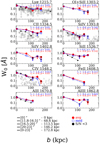 |
Fig. 6. Rest equivalent width (W0) as a function of the impact parameter (b) obtained from the line profiles in Fig. 5, corresponding to the foreground composite spectra (0 kpc) and the background composite spectra at ⟨b⟩ = 68.6 kpc (8 |


Median absorption line strengths measured (W0 Å) in stacked spectra as a function of the average impact parameter (⟨b⟩).
We note that the composite spectra considering foreground (down-the-barrel) galaxies (from our fg–bg galaxy pairs split by separation) do not show any significant dependency on the W0 of absorption lines with impact parameter b; these absorption lines show an average variance of ≤15% amongst the absorption lines included in Fig. 6. This is in agreement with the < 10% variance that Steidel et al. (2010) reported for their brightest absorption lines. Considering the background galaxies from our fg–bg galaxy pairs split by separation, our radial profiles show a general negative gradient, as reported by previous works. As the impact parameter increases, the strength of the detected absorption feature decreases. This is the case for all the spectral lines considered in our analysis. Recently, Kacprzak et al. (2021) compiled measurements of low-ionization state absorption lines (O I, C II, N II, Si II), and high-ionization state absorption lines (C III, N III, Si III, C IV, Si IV, N V, and O VI) in the CGM of low-redshift (z ≲ 0.3) galaxies with 9 ≤ log[M⋆/M⊙] ≤ 11, using quasars as background spotlights. Measurements of low-redshift galaxies (Bordoloi et al. 2018; Borthakur et al. 2015; Johnson et al. 2017; Liang & Chen 2014; Prochaska et al. 2011; Werk et al. 2013) and high-redshift galaxies (z ∼ 2.3) (Steidel et al. 2010) are also overplotted in Fig. 6.
Although at low redshift these lines can be detected at distances of up to 300 kpc, at high redshift using galaxy–galaxy pairs, Steidel et al. (2010) reported detections that are limited to 100 kpc; they included 42 additional bright quasars–galaxy pairs that provide access to the low-density gas in the CGM, and extended their Lyα detections up to 280 kpc. More recently, using galaxy images at ⟨z⟩∼2.4, Chen et al. (2020) measured the Lyα excess relative to the background intergalactic medium, probing the CGM gas up to impact parameters of 2000 kpc. Here, for star-forming galaxies at a mean redshift ⟨z⟩ = 2.6, we report detections at distances up to 146 kpc and 172 kpc for HIS and LIS–Lyα. These results include Al III, which is detected for the first time in the CGM of high-redshift star-forming galaxies up to distances of ∼150 kpc. Low-ionization state lines (C II, Si II, Al II) show less steep radial profiles compared with high-ionization lines. The LIS radial profile shows an abrupt decay at smaller radii. From separation zero to ⟨b⟩∼68 kpc, the strengths of C II, Si II, and Al II are reduced by a factor of 1.7, 2.5, and 3.2, while Si IV and C IV are reduced by a factor of 6.8 and 4.5.
Steidel et al. (2010) reported that at a separation of ⟨b⟩ = 103 kpc, lines can be hardly detected in their stacked spectra, low-ionization state metal absorption lines cannot be detected, and C IV is detected with marginal significance. Here we are able to detect LIS (C II and Si II) and HIS (Si IV, C IV) both with S/N ≥ 3 up to ⟨b⟩ = 172 kpc and 146 kpc separations. We note that beyond this separation (θ > 23″ = 172 kpc) we are unable to detect any significant signal from the background composite spectra. This might be caused by differences in the S/N and resolution of the individual spectra used in the two analyses. The spectral line features considered here are more difficult to detect in our low-resolution spectra compared to high-resolution spectra at the same S/N level. Higher-resolution spectra could resolve spectral lines that are blended (e.g. O I–Si II: λλ1303, 1307 Å, Si IV: λλ1393, 1402 Å) or that are affected by close photospheric, interstellar, or nebular spectral lines (e.g. Fe II, Fe IV: λλ1608, 1610 Å, Si II, Si II*: λλ1260, 1264 Å), disentangling the spectral features and thus providing more accurate W0 measurements. Another possibility to explain these discrepancies is that they might be the result of differences in the S/N of both parent dataset samples. We know that the two parent samples adopted opposite observational strategies. On the one hand, Steidel et al. (2004) deliberately kept the total exposure times short on their observations to maximize the number of galaxies for which redshifts could be measured. This led to a dataset with spectral quality (S/N) that varies considerably amongst their spectra (Steidel et al. 2004, 2010), and that could be affecting their redshift determinations. On the other hand, VUDS provides a homogeneous dataset with integration times of ≃14 h per target, reaching a S/N on the continuum at 8500 Å of S/N = 5 (Le Fèvre et al. 2015). Moreover, in this work we consider galaxies with reliability flags (zf = 3, 4) with 95−100% probability of being correct. However, it is not clear if similar constraints on their redshift determinations were adopted by Steidel et al. (2010) to define their galaxy–galaxy pair sample. This is crucial, as composite spectra can be affected by spectral offsets in the individual spectra. LIS and HIS spectral absorptions could be washed out or artificially boosted by considering individual spectra with low S/N and low-reliability redshift determinations to generate composite spectra. The spectra considered to generate our stacked spectra may show an average S/N higher than the average S/N of the spectra considered by Steidel et al. (2010). If similar separations ⟨b⟩ are considered, for example Steidel’s P3 sample at ⟨b⟩ = 103 kpc ( ) and this work’s S2 sample b = 113.5 kpc (
 ), Steidel’s P3 sample considers approximately five times the number of objects (N = 306) considered in our S2 sample (N = 62). This would imply that our spectra have an average individual S/N that is higher than the average S/N of the dataset used by Steidel et al. (2010), allowing us to detect similar or weaker spectral absorptions at larger separations.
To assess the correlation between W0 and b, we implemented a Kendall-Tau correlation test. The correlation coefficients rτ and the corresponding p-value (the probability of no correlation) are provided in the same figure. In all cases we find a robust anticorrelation of the strength of the absorption line as a function of the impact parameter; in particular, Lyα, C II, C IV, and Fe II all show a strong correlation (p < 0.05), while we find that O I, Si IV, Si II, Al II, and Al III present a flatter radial profile, which results in a lower significance of the anticorrelation (p ∼ 0.1). To assess the scale of the relationship between W0 and b, we computed the slopes of the radial profiles shown in Fig. 6. We find that Lyα shows a slope of −1.20 ± 0.01; LIS (O I + Si II, C II, Si II, Fe II, and Al II) absorption lines show slopes of −1.34 ± 0.01, −1.31 ± 0.01, −1.53 ± 0.02, −1.50 ± 0.07, and −1.44 ± 0.05, respectively; Al III shows a slope of −1.38 ± 0.06; and HIS (Si IV and C IV) absorption lines show slopes of −1.10 ± 0.04 and −1.24 ± 0.01. If we focus on low- and high-ionization lines of the same species, and consider Si II–Si IV and C II–C IV absorption line pairs, we find that the slopes of these absorption lines are different at ≥ 5σ level. Compared with the Steidel et al. (2010) radial profiles, our results show slopes that are different at a 5σ level for Si II and at a 3σ level for C II and Al II absorption lines. These differences suggest that within the CGM, cold and dense gas is more spatially extended in galaxies at z ∼ 2.6 compared with galaxies at z ∼ 2.3 and lower redshifts, as probed by Si II C II, in agreement with the expected higher covering factors of neutral gas at higher redshifts (Reddy et al. 2016; Du et al. 2018; Sanders et al. 2021). Compared with low-redshift CGM studies (see Fig. 6), our Lyα, LIS, and HIS rest-frame equivalent width radial profiles are at the upper envelope of the equivalent width measurements at lower redshifts, suggesting a potential redshift evolution for the CGM gas content that produces these absorptions.
4.2. Star formation and stellar mass dependence
To explore the dependence of low- and high-ionization state absorptions with physical and morphological properties (i.e. star formation rate, stellar mass, galaxy effective radius, and azimuthal angle) produced in the CGM of our high-redshift star-forming galaxy sample, we considered galaxy pairs at all projected distances (b < 23″) split by the corresponding galaxy property. A summary of the statistical properties of the galaxy pair subsamples divided by these properties can be found in Appendix A. We note that the Fe II, Al III, and Al II lines were excluded from our following analyses (see Sect. 4.1). Figure 7 (upper panels) shows the equivalent width of the absorption features as a function of stellar mass and SFR for LIS (C II, Si II), HIS (Si IV, C IV), and Lyα. We find that galaxies with high stellar masses (log[M⋆/M⊙] > 10.30) and high star formation rates (log[SFR/(M⊙ yr−1)] > 1.93) show C IV (HIS) metal absorption with larger equivalent widths. On the other hand, galaxies with low stellar masses (log [M⋆/M⊙] < 9.26) and low SFRs (log[SFR/(M⊙ yr−1)] < 0.9) show C II (LIS) metal absorptions with stronger equivalent widths. Nevertheless, Si II and Si IV do not show a similar trend. This might be caused by the fact that we do not have Si II and Si IV detections with S/N > 3 in all of our SFR and stellar mass bins.
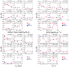 |
Fig. 7. Rest equivalent width (W0) of the absorption lines as a function of the foreground galaxy’s stellar mass (log[M⋆/M⊙]), SFR (log[M⊙ yr−1]), effective radius (reff), and azimuthal angle (ϕ). The W0 measurements come from composite spectra considering galaxy pairs at all projected distances (b < 23″) and split by the corresponding galaxy property. Stellar mass and SFR W0 were obtained from composite spectra considering 238 bg galaxies, while reff and ϕ come from composite spectra considering 97 bg galaxies (see Sect. 2 and Table 2). Average and median W0 are shown in solid red and open blue symbols; solid black symbols correspond to upper limits with S/N < 3. The error bars correspond to 1σ confidence intervals for average or median values based on a bootstrap analysis. The panels include the results from the Kendall-Tau correlation test: the correlation coefficients rτ and their corresponding p-value (the probability of no correlation). The panels of absorption lines with detections in only two subsamples also show the results from a Student’s t-test: the difference between a pair of mean values given by the t coefficient and their corresponding p-value (the probability of significant difference amongst means). |
To quantify the robustness of the trends highlighted in Fig. 7, we ran a Kendall-Tau rank test for the absorption lines that are detected in at least three bins. We find that SFR and stellar mass are anticorrelated with C II, but they correlate positively with C IV. This would imply that C II is located mostly in galaxies with low stellar mass(log[M⋆/M⊙] < 9.26) and low SFR (log [SFR/(M⊙ yr−1)] < 0.9), while C IV is detected in galaxies with high stellar mass (log[M⋆/M⊙] > 10.2) and high SFR (log [SFR/(M⊙ yr−1)] > 1.5). The slopes of the W0 relationships with stellar mass and SFR for C II and C IV are 0.79 ± 0.13, 0.61 ± 0.05 and 0.73 ± 0.08, 0.55 ± 0.04, which are significantly different at ≥5σ level. We do not find any robust correlation between SFR and stellar mass with Si II, Si IV, Fei II, Al II, Al III, or Lyα, yielding a probability of no correlation above 60% in all cases. We also explored the combined effect of impact parameter with stellar mass and SFR; however, no clear conclusion was reached due to the low number statistics, which resulted in composite spectra with low S/N line detection.
4.3. Morphological dependence
The strength of the observed metal absorption signatures in the CGM can be explored as a function of the azimuthal angle ϕ between the l.o.s. and the projected major and minor axes of the foreground galaxy. Here we define the azimuthal angle (ϕ) as the projected angle between the background galaxy l.o.s. and the projected minor axis of the foreground galaxy. Small azimuthal angles (ϕ ∼ 0°) refer to l.o.s. passing along the projected minor axis of the foreground galaxy, while large azimuthal angles (ϕ = 90°) refer to l.o.s. passing along the projected major axis of the foreground galaxy. The effective radius ( 4) was obtained by fitting a single Sérsic profile with no constraints on the parameters, and then was circularized using the galaxy ellipticity (Ribeiro et al. 2016). Alongside the effective radius, GALFIT provides other structural parameters: Sérsic index (n), the axis ratio of the ellipse (b/a), and the position angle, θPA. Out of the 238 galaxies evaluated in this paper, only 97 are in the COSMOS field and covered by HST imaging, and therefore have morphological parameters. To inspect the dependency of the LIS-HIS absorption strengths with the azimuthal angle (ϕ), we split our sample into three ϕ bins: [0−30]°, [30−60]°, and [60−90]°. Figure 7 (lower panels) reports the equivalent widths of different spectral features in bins of reff and ϕ.
To check and assess the robustness of possible correlations between the morphological parameters and the equivalent widths measured in the composite spectra for LIS, HIS, and Lyα, we ran a Kendall-Tau rank test between W0 and ϕ and reff. For lines detected in only two bins the correlation cannot be assessed; therefore, we estimated the significance of the difference between their absorption strength (W0). To do this we applied a Student’s t-test to determine the probability that the W0 variations between the low and high reff and ϕ populations are not statistically significant. According to the Student’s statistics (t) a large p-value indicates to a high probability that the null hypothesis is correct (the two samples are not statistically significant); a small p-value suggests that the difference is significant. The Kendall-Tau and Student’s t-test results are both given in Fig. 7 in the corresponding panels.
For the effective radius (reff) of the galaxy, the Kendall-Tau test shows a mild anticorrelation with C II (p < 0.117), while it does not show any significant correlation with Si II and Si IV (p > 0.602). We find a significant difference (p < 0.01) in the W0 variations between small and large reff as shown by the Student’s t-test. However, no correlation is found for Lyα. This suggests that C IV gas is usually located in the CGM of larger galaxies, while C II gas is located in the CGM of smaller galaxies. Concerning the azimuthal angle, we do not find any significant correlation with ϕ in any of the spectral lines inspected in agreement with what has been reported by (Chen et al. 2021), who inspected the azimuthal dependence of Lyα emission of 59 star-forming galaxies (zmed ∼ 2.3). This is opposed to the low-redshift scenario where galaxies show high-velocity biconical outflows oriented along the minor-axis and accreting material along the major-axis. This result could be linked to the metal distribution along the disc of star-forming galaxies as metal absorption systems are often compact and poorly mixed, where cool low-ionization metal absorbers have typical sizes of ∼1 kpc (Faucher-Giguère 2017a), while high-ionization gas seen in absorption arises in multiple extended structures spread over ∼100 kpc (Churchill et al. 2015; Peeples et al. 2019).
4.4. C II/C IV line ratio
A further inspection of the differences between LIS and HIS on the different galaxy parameters come from the C II/C IV equivalent width line ratio. We focus on carbon ions as they provide stronger absorptions with higher S/N compared to aluminium or silicate ions. Figure 8 shows the C II/C IV line ratio as a function of impact parameter, stellar mass, and star formation rate. The C II/C IV line ratio appears to anticorrelate with impact parameter (b), stellar mass, and star formation rate. Similarly to the analyses for individual line absorptions, we ran a Kendall-Tau to assess possible correlations for C II/C IV line ratio and included it in all panels of Fig. 8. We confirm that the anticorrelations between C II/C IV ratio and impact parameter, stellar mass, and star formation rate are statistically robust. This suggests that C II is more important than C IV in the inner regions of these star-forming galaxies, while the opposite occurs in the outskirts at large separations.
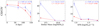 |
Fig. 8. CII/CIVW0 line ratio as a function of the impact parameter b, and the foreground galaxy’s stellar mass and SFR. CII/CIVW0 values were obtained considering the same set of fg–bg galaxy pairs. Average and median W0 are shown in solid red and open blue symbols; the solid black symbols correspond to upper limits with S/N < 3. The error bars correspond to 1σ confidence intervals for average or median values based on a bootstrap analysis. |
On the other hand, star-forming galaxies and low stellar mass with low star formation rates show a higher CII/CIV line ratio compared with galaxies that have high stellar mass and high star formation rates. Our results suggest that galaxies with higher star formation rates and large stellar masses are capable of sweeping out the highly ionized gas (traced by C IV) farther away from the galaxy compared with less actively star-forming and less massive galaxies. Another possible explanation is that more active and massive galaxies have stronger ionizing fluxes, able to ionize gas at larger distances compared with less massive and less active galaxies. Recent studies have shown that fast and energetic outflows can push material away from the central regions in star-forming galaxies, more effectively in galaxies with high SFR (with a weaker dependence on stellar mass; Heckman et al. 2015; Cicone et al. 2016; Trainor et al. 2015; Feltre et al. 2020). The presence of an AGN can make this effect even more dramatic, as shown by an enhanced gas budget in H I and low-ionization gas in high-redshift (z > 2) galaxies (Prochaska et al. 2014), suggesting higher accretion rates or a net gain of cold gas in the CGM in these star-forming galaxies (Faucher-Giguère et al. 2016). However, the physical mechanism through which the AGN removes and/or heats the gas and suppresses accretion is not clear (Tumlinson et al. 2017). Determining the nature of the source responsible for ionizing the gas in the CGM is crucial to improving our understanding of the multi-phase CGM, but is beyond the scope of this paper.
4.5. Lyα emission
As we already noted in Sect. 4.1 (Fig. 5), the Lyα emission component is clearly detected in our composite spectra. Figure 9 shows the Lyαem rest equivalent width as a function of the impact parameter. We find that Lyαem decreases as a function of the impact parameter b similarly to what Chen et al. (2021) reported from 2D Lyαem maps. We also explore the Lyαem equivalent width strength as a function of the galaxy stellar mass, star formation rate, and azimuthal angle. However, we do not find any significant correlation in these cases. This might be caused by the fact that at z ∼ 2 the Lyαem–stellar mass relation is weaker compared with galaxies at higher redshifts (Du et al. 2018). Another possibility is that our Lyαem measurements come from composite spectra, hence from star-forming galaxies with and without direct Lyαem detections (EW ≤ 0 Å, EW > 0 Å and EW ≥ 20 Å Le Fèvre et al. 2015; Hathi et al. 2016), covering a wide range of stellar masses and star formation rates that may have diluted a real Lyαem signal (Steidel et al. 2011).
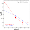 |
Fig. 9. Equivalent width (W0) for the Lyα emission as a function of the impact parameter (b) obtained from the average (solid red line) and median (dot-dashed blue line) composite spectra. The error bars correspond to 1σ confidence intervals for average or median values based on a bootstrap analysis. |
5. Discussion
Analyses of low- and high-ionization state absorption features and their dependence on stellar mass, star formation rate, and galaxy inclination have been widely explored at ≲0.5 (see Tumlinson et al. 2017; Kacprzak 2017). At high redshift, however, the studies of the CGM are limited. Steidel et al. (2010) used 512 close (< 15″ = 124 kpc) angular pairs of z ∼ 2 − 3 (zbg ∼ 2.3) galaxies to map the cool and diffuse gas around galaxies. They found strong evidence suggesting the presence of superwind outflows, and proposed a simple model of the gas in the CGM, where cool gas is distributed symmetrically around every galaxy, accelerating radially outwards with the outflow velocity increasing with radius. Later, Turner et al. (2014) and Lau et al. (2016) reported detections that suggest that in galaxies at ⟨z⟩ = 2.4 the CGM extends at least up to 180 kpc. Moreover, the mass of metals found within the halo is substantial and equivalent to ∼25% of the metal mass within the interstellar medium (Rudie et al. 2019). This is, however, a lower percentage than what has been reported from studies in low-redshift galaxies (Werk et al. 2014), which suggests a considerable redistribution of the metal content of galaxies in an inside-out fashion over the last ∼8.5 Gyr. We note that eight of the nine resonance Si II transitions fall within the [900−1900] Å wavelength range considered here: λ989 Å, λ1020 Å, λλ1190, 1193 Å, λ1260 Å, λ1304 Å, λ1526 Å, and λ1808 Å (Shull et al. 1981). Lines located bluewards of Lyα are not included in our analyses as the result of the low coverage of our composite spectra at this wavelength range and because UV continuum level bluewards of Lyα is particularly sensitive to the dust content, metallicity, and the age of the stellar population (Trainor et al. 2015) and their strength could be affected by IGM absorptions (Shapley et al. 2003). The Si II (λ1304 Å) component is blended with the O I (λ1302 Å) absorption line and is close to excited fine-structure emission transitions that could lower the W0 measurements (Trainor et al. 2015). Finally, Si II (λ1526 Å) is the least resonance component affected by blends (Shapley et al. 2003) and is the strongest Si II line amongst their counterparts. For this work we chose λ1526 Å for our Si IIW0 computations as this component is free of blending effects caused by the low spectral resolution of our dataset. However, as noted by Jones et al. (2018) Si II transitions probe diverse optical depths, and hence the most accurate way to compute Si II absorption strength is to consider the contributions of all the Si II resonance components (λλλ 1260, 1304, 1526 Å) within the analysed range, by averaging their strengths and deblending them from nearby spectral features that could affect their individual W0 measurements. Nevertheless, different studies have adopted diverse strategies to compute the LIS (including Si II resonance components) W0 strength. For example, Jones et al. (2018) averaged Si II (λλλ 1260, 1304, 1526 Å), O I (λ1302), C II (λ1334 Å), Al II (λ1670 Å), Fe II (λ2382 Å), and Mg II (λλ2796, 2803 Å) components; Ranjan et al. (2022) considered the average of the eight Si II resonance components to estimate the W0 Si II absorption in high-z damped Lyman-α (DLA) systems; Du et al. (2016) averaged Si II (λ1526 Å), Al II (λ1670 Å), Ni II (λλ1741, 1751 Å), Si II (λ1808 Å), and Fe II (λ2382 Å) absorption lines to compute an overall LIS average absorption estimation, while later Du et al. (2018) considered Si II (λ1260 Å), O I–Si II (λλ1302, 1304 Å), C II (λ1334 Å), and Si II (λ1526 Å) for similar computations. The differences in the number of Si II resonance components considered for W0 computations could be the reason why similar Si II trends to those of C II with SFR and stellar mass shown in Fig. 7 are not appreciated. As shown by Jones et al. (2018) different low ion transitions (Si II, Fe II, and Ni II) show non-uniform covering fractions in the CGM of star-forming galaxies at high redshift (z ≃ 2 − 3).
In this work we used a sample of 238 galaxy close pairs to probe the CGM around star-forming galaxies at z ∼ 2.6. Our results show an anticorrelation between the equivalent width of the absorption lines and the impact parameter (b) for this high-redshift star-forming galaxy sample and are consistent with previous results at lower redshift. Here we detect Lyα–LIS and HIS absorption at distances up to 172 kpc and 146 kpc. Our low-ionization state (C II, Si II), and high-ionization state (C IV Si IV) absorption line detections shape an upper envelope of the equivalent width distribution coming from studies at low redshift (see Fig. 6). This is further illustrated by the differences in the slopes of the W0 radial profiles between low- and high-ionization state absorptions of the same ion species, where Si II–Si IV and C II–C IV absorption line pairs are different at a ≥5σ level. Moreover, when compared with galaxies at z ∼ 2.3 (Steidel et al. 2010) our results show a significant difference in their slopes at a 5σ level for Si II and a 3σ level for C II and Al II absorption lines. These discrepancies between LIS and HIS suggest that, within the CGM, cold (T < 104.5 K) and dense gas is more extended in galaxies at z ∼ 2.6 compared with galaxies at z ∼ 2.3 and lower redshifts, as probed by Si II, C II, Si IV, and C IV. These results suggests a potential redshift evolution for the CGM gas content that produces these absorptions. As higher covering factors of neutral gas lead to stronger absorption lines (Du et al. 2018), this suggests a higher content of neutral gas in high-redshift galaxies compared with low-redshift galaxies. This concentration of neutral gas could represent a reservoir of gas that can be later accreted onto the galaxies to fuel future star formation (Hafen et al. 2019, 2020).
We note that it is possible to increase the maximum angular projected separation (≥23″) allowing us to probe larger distances closer to the CGM and IGM boundary, following Chen et al. (2020). However, we limited our analyses to 23″ ∼ 170 kpc and galaxy spectra with highly reliable redshifts to guarantee detection with good S/N. Spectra with unreliable redshift measurements could wash out the expected metal absorptions and/or produce spurious features in the final composite spectra. This is further supported by the observed metallicity dependence with impact parameter, where LIS are preferably located in the inner CGM (close to the galaxy; Lau et al. 2016), while HIS (e.g. O VI are expected to dominate the CGM at larger separations Shen et al. 2013) making it difficult to detect weak LIS absorptions at larger separations given their expected W0.
5.1. LIS and HIS absorption dependencies
At z ≲ 1, Churchill et al. (2000) explored a sample of 45 Mg II absorption systems in high-resolution QSO spectra, and studied their spectra, together with the C IV and Fe II absorption profiles, suggesting that the gas responsible for Mg II and C IV absorptions arises from gas in different phases (i.e. gas producing HIS absorption features have typical temperatures T > 105 K Tumlinson et al. 2017). Moreover, they observed an evolution of the absorbing gas that is consistent with scenarios of galaxy evolution in which mergers and accretion of ‘protogalactic clumps’ provide gas reservoirs responsible for the elevated star formation activity at high redshift, while at intermediate and lower redshifts (z ≤ 1), the balance of high- and low-ionization state CGM gas may be related to the presence of star-forming regions in the host galaxy (Churchill et al. 2000). Later on, Zibetti et al. (2007) found that early-type (quiescent, red) galaxies (0.37 < z < 1) are associated with weaker Mg II absorptions, while stronger systems are located in late-type (star-forming, blue) galaxies. These results provided evidence that the SFR correlates with Mg II absorption strength caused by the presence of outflows from star-forming or bursting galaxies. This scenario is also supported by subsequent studies that demonstrated that SFR correlates with outflow velocity deduced from the Mg II absorption strength (Weiner et al. 2009; Martin et al. 2012; Tremonti et al. 2007; Rubin et al. 2010), and by the correlation between the stellar mass and Lyα absorption strength (Bordoloi et al. 2018; Wilde et al. 2021).
Our detection of LIS and HIS absorption lines suggests that at ⟨z⟩∼2.6 the C II and C IV features are correlated with star formation rate and stellar mass. C II is stronger in galaxies with low star formation rates and low stellar masses, while C IV is stronger in galaxies with high SFR and high stellar masses. These results are consistent with what has been reported for low-redshift galaxies in scenarios where LIS and HIS absorbers have different spatial distributions. Low-ionization state metal absorbers probe the gas that is less ionized than high-ionization state metal absorbers (Nagao et al. 2006), and thus they are expected to be located in gas regions with different density conditions (Burchett et al. 2016). Moreover, studies of low-redshift galaxies (z ≤ 0.5) have shown that as a consequence of the interaction between a starburst-driven wind and the preexisting CGM at radii as large as 200 kpc, the CGM around star-forming galaxies with high star formation rates differs systematically compared to galaxies with lower SFRs, as probed by the Lyα, Mg II, Si II, C IV, and O VI absorption lines (Tumlinson et al. 2011; Borthakur et al. 2013; Lan et al. 2014; Heckman et al. 2017). However, as suggested by Cicone et al. (2016) and Gatkine et al. (2022), their correlation with stellar mass and star formation rate might in fact be a consequence of a main-sequence offset, rather than simply a correlation with star formation rate or stellar mass, and because LIS–HIS covering factors can be affected by environmental processes (Dutta et al. 2021). Hence, caution should be taken when interpreting LIS–HIS correlations with SFR and/or stellar mass.
The origin of the reservoir of cold neutral gas around low stellar mass galaxies and low SFRs at these distances(⟨b⟩≈120 kpc; see Appendix A) is uncertain. One explanation comes from a soft radiation field unable to ionize HIS (i.e. C IV, Si IV) as the production of C IV and Si IV absorption features in the CGM requires photons with energies > 45 eV associated with hard ionizing radiation fields from massive stars, AGN, and radiative shocks (Feltre et al. 2020; Trainor et al. 2015). As shown by Gatkine et al. (2022), HIS are more affected by high-velocity outflows; they show a strong correlation with SFR and are ubiquitous in high-SFR systems. Another possible explanation comes from the galactic fountain scenario, predicted by cosmological galaxy formation simulations (Oppenheimer et al. 2010; Vogelsberger et al. 2013), where the presence of cold low-ionization gas results from metal-rich gas ejected in previous star formation episodes that fall back to the disc (Fraternali & Binney 2006; Hobbs et al. 2015). Moreover, we know that stellar winds are dominant in the inner region of the CGM < 60 kpc (Chen et al. 2020), and depending on their velocity, stellar winds in low-mass galaxies might be able to expel material or be reaccreted as recycled material (Sánchez Almeida 2017). However, if the velocity outflow is insufficient to eject material out into the IGM, the recycle timescales in low-mass galaxies where gas returns to the galaxy can be as small as those in high-mass systems (van de Voort 2017). Martin et al. (2012) detected Fe II Doppler shifts and Vmax–Mg II values that suggest that outflows reach the circumgalactic medium with Mg II absorption at blueshifts as high as 700 km s−1, reaching 70 kpc in 100 Myr, a short enough time for the host galaxy to sustain SFR, even if the SFR declines due to an outflow. Nevertheless, our measurements do not allow us to break down the multiple components of the absorption features in our foreground galaxy (down-the-barrel) composite spectra and to detect blueshifted offsets that could be related to high-velocity outflows. We note that it is possible to combine down-the-barrel and QSO–galaxy and/or galaxy–galaxy pairs to unambiguously detect blueshifted absorptions relative to the galaxy systemic velocity, and quantify independently the main properties of the detected outflow (Kacprzak et al. 2014; Bouché et al. 2016; Lehner 2017).
Figure 7 (lower panels) shows the dependence of line absorption strength on the galaxy’s effective radius (reff) and azimuthal angle (ϕ). For the dependence of the absorption strength (W0) on the size of the galaxy given by the effective radius(reff), we find that LIS absorptions are stronger in smaller galaxies compared to HIS absorptions, which are shown to be stronger in larger galaxies, in agreement with Rudie et al. (2019), who reported that LIS absorption occurs spatially closer to the galaxy, and gas producing HIS absorptions can be located well beyond the virial radius. Regarding the dependence on azimuthal angle, we do not find any significant correlation with ϕ for either LIS or HIS. However, these results are based on the fraction of galaxies for which we have morphological measurements (∼40% of the parent sample). Thus, these results have to be confirmed by a similar morphological analysis using larger samples at these high redshifts, as galaxy orientation plays a major role in the measured strength of LIS and HIS. This has been shown at low redshift from studies using analyses of down-the-barrel (Rubin et al. 2014; Bordoloi et al. 2014b) and QSO–galaxy pairs (Kacprzak et al. 2011; Bordoloi et al. 2011). Moreover, at z ≳ 2 star-forming galaxies have clumpy morphologies (Förster Schreiber et al. 2011), with galactic winds that are mainly driven by outflows from prominent star-forming clumps (Genzel et al. 2011), and have not yet formed a stable disc (or any disc at all) capable of collimating galactic winds into bipolar outflows (Faucher-Giguère 2017b), indicating that the minor–major axis dichotomy associated with rotation present at low redshift (z < 1) is not broadly applicable at z ∼ 2 − 3 (Law et al. 2012; Nelson et al. 2019; Price et al. 2020). Therefore, it is not obvious that at high redshift (z ≳ 2) the azimuthal angle can be determined and, if it can, whether it has any physical meaning.
The dependence of LIS and HIS absorption strength on the azimuthal angle has been explored in the literature to prove or disprove theories on how galaxies accrete gas from the intergalactic medium. Inflowing material along filaments in the IGM is expected to be the largest source of accretion (Kereš et al. 2005). Simulations have shown that accretion of metal-poor gas inflows occurs along the major axis of galaxies, where outflows that are preferably located along the semi-minor axis form bipolar outflows (Putman 2017), and gas being accreted onto galaxies that can later trigger star formation has been supported by evidence collected from multiple CGM studies at low redshift (Kacprzak et al. 2010, 2012, 2015, 2019; Lan & Mo 2018; Martin et al. 2019; Nielsen et al. 2015; Rubin et al. 2018; Zhu & Ménard 2013; Tumlinson et al. 2011; Bordoloi et al. 2014a; Lan et al. 2014). Recent cosmological hydrodynamical simulations examine the physical properties of the gas located in the CGM of star-forming galaxies as a function of angular orientation by Péroux et al. (2020). They found that the CGM varies strongly with impact parameter, stellar mass, and redshift. Moreover, they suggest that the inflow rate of gas is more substantial along the galaxy major axis, while the outflow is strongest along the minor axis.
The correlations between C II and C IV with impact parameter, star formation rate, and stellar mass scenario of a multi-phase CGM(where LIS absorptions are produced by denser gas located closer to the galaxy, whether this dense neutral gas component is part of an outflow or material falling back to the galaxy taking part in a galactic fountain that could eventually be funnelled to the galaxy to sustain star formation activity; Kereš et al. 2005) is not clear and cannot be assessed by our datasets. On the other hand, HIS absorption features associated with strong stellar winds produced by high star formation activity capable of ionizing radiation in high stellar mass galaxies with high star formation activity sweeping material to the outer regions of these galaxies (Putman 2017; Bower et al. 2016; Oppenheimer et al. 2016; Voit et al. 2015).
Similar analyses including observations at different redshifts coming from different complementary surveys, for example VANDELS (McLure et al. 2018; Pentericci et al. 2018), zCOSMOS (Lilly et al. 2007, 2009), VVDS (Le Fèvre et al. 2013), and DEIMOS10K (Hasinger et al. 2018), can help to increase the number of galaxy pairs with close angular separations (b < 6″), deblend close spectral line features (e.g. C II–O IVλλ1334.5, 1343.0 Å; Si IVλλ1393.8, 1402.8 Å), and cover different low- and high-ionization state lines(e.g. O VIλλ1032, 1038 Å, Mg IIλ2798 Å). Additionally, it has been shown that AGN activity is dependent on stellar mass and SFR (e.g. Lemaux et al. 2014; Bongiorno et al. 2016; Magliocchetti et al. 2020), and thus studies considering bg–AGN and/or QSO–AGN galaxy pairs (Hennawi et al. 2006; Prochaska et al. 2014) are needed to study the effect that the presence of an AGN has on feedback and quenching in star-forming galaxies at low and high redshifts.
5.2. C II/C IV line ratio
A further inspection of the differences between LIS and HIS on the different galaxy parameters explored comes from the C II/C IV line ratio. We find that C II/C IV line ratio anticorrelates with impact parameter, stellar mass, and star formation rate. This implies that C IV is mostly located at larger distances in more massive galaxies with higher star formation rates, while C II dominates at smaller impact parameters and is found mostly in low stellar mass galaxies with low star formation rates. These results further support the picture of a multi-phase CGM where LIS line absorptions are produced by denser gas with lower temperatures (T < 104.5 K) that is located close to the central galaxy, while HIS line absorptions are produced by warm gas located at larger distances from the central galaxy. Simulations have shown that much of the ongoing gas accretion occurs towards the edges of the galaxies to avoid the dominant feedback (outflows) from the central regions (Stewart et al. 2011; Fernández et al. 2012; Putman 2017); however, we do not find supporting evidence of the low-redshift scenario where low-ionization state gas infalls along the major axis of star-forming galaxies, accompanied by large-scale outflows along the minor axis forming bipolar outflows. On the contrary, our results suggest that this scenario is not broadly applicable at z ∼ 2. We note that we have also explored Si II/Si IV and Al II/Al III equivalent width line ratios; however, we did not detect any significant correlations. On the one hand, Si IV predominantly arises in denser gas closer to galaxies more similar to other LIS state lines such as Mg II than to those of higher ions (Ford et al. 2013, 2014), and hence Si II and Si IV line absorption might be probing gas with similar physical conditions. On the other hand, Al III is an intermediate-ionization state (IIS) tracer of moderately photoionized warm gas generally associated with neutral phase gas (Savage et al. 2001; Knauth et al. 2003; Vladilo et al. 2001). In fact, Al III absorption is associated with low ions, as shown by the significant correlation between the velocity widths of Al III and low-ionization species (e.g. Si II, Fe II, Zn II, Howk et al. 1999), suggesting that a substantial fraction of the low-ionization ions may be associated with moderately ionized gas traced by Al III and Fe III (Wolfe et al. 2005) and that doubly ionized species (e.g. Al III, Fe III, C III, Si III) often have comparable column densities to the singly ionized species (e.g. Al II, Fe II, C II, Si II) (Mas-Ribas et al. 2017).
5.3. Lyα emission
Regarding Lyαem, several studies have been carried out to explore the relation with galaxy properties. At low redshift Runnholm et al. (2020) used the Lyman Alpha Reference Sample (LARS) to obtain correlations between Lyα and different galaxy properties (i.e. star formation rate, dust extinction, compactness, and the gas covering fraction). At high redshift it has been found that bluer galaxies show stronger Lyαem (Shapley et al. 2003; Pentericci et al. 2010; Berry et al. 2012; Erb et al. 2016), and that low stellar mass galaxies with lower SFRs show stronger Lyαem than high-stellar mass galaxies with higher SFRs (Vanzella et al. 2009; Stark et al. 2010; Erb et al. 2006; Jones et al. 2012; Shapley et al. 2003; Kornei et al. 2010; Hathi et al. 2016). Additionally Lyαem is correlated with LIS absorption; stronger LIS absorptions correspond to weaker Lyαem, as high concentrations of neutral gas responsible for strong LIS absorption are also responsible for scattering out of the l.o.s. Lyα photons (Shapley et al. 2003; Vanzella et al. 2009; Jones et al. 2012). More recently, Du et al. (2018), Trainor et al. (2019), and Pahl et al. (2020) studied the spectroscopic properties of star-forming galaxies at z ∼ 2 − 5 through composite spectra grouped through different galaxy properties. They detected stronger Lyαem at higher redshift at fixed stellar mass, SFR, and UV luminosity, and found that the LIS–Lyαem relation is redshift independent, suggesting that this is caused by the variations of the neutral gas covering fraction favouring Lyα escape and production and/or dust content in the ISM and CGM. Moreover Oyarzún et al. (2016, 2017) show that at high redshift (3 < z < 4.6) the Lyαem anticorrelations with stellar mass, star formation rate, and UV luminosity are stronger in low stellar mass populations, which is explained by the rapidly increasing neutral gas fraction of the universe at higher redshifts (Du et al. 2021).
6. Conclusions
In this paper we presented stacks of 238 background galaxy spectra used to probe the CGM content and extent around star-forming galaxies at ⟨z⟩∼2.6. We only used spectra with highly reliable spectroscopic redshifts (95 − 100% probability of being correct) to identify the low-ionization state (LIS: Si II, C II) and high-ionization state (HIS: C IV, Si IV) metal absorption lines, and constrain their spatial distribution and their dependence on stellar mass, star formation rate, azimuthal angle, and effective radius.
We summarize our main results below:
-
We detect LIS and HIS metal absorption lines in the CGM around star-forming galaxies at distances up to 172 kpc and 146 kpc, respectively. The limitations owing to the size of our sample did not allow us to follow metal lines beyond these distances. The strength of these absorptions decreases at increasing distances from the galaxy, consistently with results published in the literature. At any fixed distance from the galaxy, the strength of all absorption lines that we identify in our sample at z ∼ 2.6 is greater than any other measurement at lower redshift, providing evidence of a redshift evolution of the CGM gas content responsible for producing these absorptions.
-
We do not find any significant correlation between the LIS–HIS absorptions and the azimuthal angle (ϕ). This is opposed to the scenario at low redshift where cold gas (traced by LIS line) is infalling onto galaxies along the plane containing the disc, while the gas heated and processed by star formation (traced by HIS lines) is outflowing perpendicularly to the plane. This can be explained by the fact that high-redshift galaxies have not formed a stable disc capable of collimating galactic winds into bipolar outflows. However, due to the small sample of close pairs with available morphological features, these trends need to be confirmed by applying a similar analysis to larger samples at these high redshifts.
-
We find an anticorrelation between Lyαem and the impact parameter b, in agreement with previous results at high redshift.
-
To assess the relative importance of LIS and HIS absorptions, we computed the CII/CIV equivalent width line ratio and find that it correlates with impact parameter b, stellar mass, and star formation rate. The CII/CIVW0 line ratio is higher at small separations, mainly detected in star-forming galaxies (⟨z⟩∼2.6) with low stellar masses and low star formation rates. Conversely, low CII/CIV line ratios are defined by stronger CIV line absorption compared to CII and are observed at large separations in star-forming galaxies with higher stellar masses and star formation rates.
The results presented here provide observational evidence consistent with a scenario where star-forming galaxies at ⟨z⟩∼2.6 possess a multi-phase CGM where LIS metal absorptions are produced by denser gas, which is more extended in these star-forming galaxies. Our results suggest that galaxies with higher star formation rates and high stellar masses have stronger ionizing fluxes that are able to ionize gas at larger distances and/or are capable to sweep out the highly ionized gas (traced by C IV) farther away from the galaxy compared with less massive and less star-forming galaxies. Subsequently, star-forming galaxies with low SFR and low stellar mass show larger reservoirs of cold gas as probed by their C II and C IV lines and their C II/C IV equivalent width line ratio. These large reservoirs of cold gas could be funnelled into the galaxies and eventually provide the necessary fuel to sustain star formation activity. Recently, Wang et al. (2022) has demonstrated that large-scale environment modulates star formation by regulating the way in which galaxies breathe material in and out (accrete and expell) by exchanging material within the CGM. This process is synchronized with star formation rate events occurring within a galaxy, and is related to maxima (minima) of SFR associated with a previous decrease (increase) in the cold circumgalactic gas phase, that halts a further rise (decline), and leads to a fall (rise) in the star formation rate at later stages. Our results from C II peaks and C IV troughs detected in low-mass galaxies (low SFRs) and high-mass galaxies (high SFRs) could be interpreted as the snapshots of these two different stages of the complex interplay between the ISM, CGM, and IGM in which galaxies exchange material. However, we note that high-resolution observations are required to detect outflows expelling material or inflows accreting cold material back to the galaxy as recycled material. We highlight that although stacking increases the S/N of the background spotlights, allowing us to detect the faint signal produced by gas in the CGM, it also smears out the information about the spatial, kinematic, and ionization properties of the CGM. Thus, we reiterate the necessity to perform deeper observations with higher resolutions at this and higher redshift of multiple LIS and HIS metal lines to provide better constraints on the properties of the multi-phase CGM. It is very likely that future and ongoing observations from large and deep spectroscopic surveys such as VANDELS (McLure et al. 2018; Pentericci et al. 2018), zCOSMOS (Lilly et al. 2007, 2009), VVDS (Le Fèvre et al. 2013) or DEIMOS10K (Hasinger et al. 2018) and Integral Field Unit observations from MUSE/KMOS/JWST will help us understand more about the multi-phase nature of the CGM. Future work should point towards a resolved view of the velocity field of the in-falling and out-flowing gas of galaxies at redshift z > 2.
Full observed wavelength coverage of 3650 < λ < 9350 [Å], which at z ∼ 2.6 translates into a rest-frame wavelength coverage of 1013 < λ < 2597 [Å].
We made use of PYSYNPHOT (Blagorodnova et al. 2014) to resample our spectra.
q is the axis ratio (b/a) of the elliptical isophotes that best fit the galaxy.
Acknowledgments
We thank an anonymous referee for constructive comments and suggestions that improved the manuscript. Based on data obtained with the European Southern Observatory Very Large Telescope, Paranal, Chile, under Large Programs 175.A-0839, 177.A-0837, and 185.A-0791. This work is based on data products made available at the CESAM data center, Laboratoire d’Astrophysique de Marseille. This work partly uses observations obtained with MegaPrime/MegaCam, a joint project of CFHT and CEA/DAPNIA, at the Canada-France-Hawaii Telescope (CFHT) which is operated by the National Research Council (NRC) of Canada, the Institut National des Sciences de l’Univers of the Centre National de la Recherche Scientifique (CNRS) of France, and the University of Hawaii. This work is based in part on data products produced at TERAPIX and the Canadian Astronomy Data Centre as part of the Canada-France-Hawaii Telescope Legacy Survey, a collaborative project of NRC and CNRS. H.M.H. acknowledge partial support from National Fund for Scientific and Technological Research of Chile (Fondecyt) through grants no. 1171710 & 1150216. E.I. acknowledges partial support from FONDECYT through grants N° 1221846 and 1171710. M.A. acknowledges support from FONDECYT grant 1211951, “ANID+PCI+INSTITUTO MAX PLANCK DE ASTRONOMIA MPG 190030” and “ANID+PCI+REDES 190194”. R.A. acknowledges support from ANID FONDECYT Regular Grant 1202007. We thank ESO staff for their support for the VUDS survey, particularly the Paranal staff conducting the observations and Marina Rejkuba and the ESO user support group in Garching. This research used Astropy (http://www.astropy.org), a community-developed core Python package for Astronomy (Astropy Collaboration 2013, 2018), Numpy (Harris et al. 2020), Scipy (Virtanen et al. 2020) and Matplotlib (Hunter 2007).
References
- Adelberger, K. L., Steidel, C. C., Shapley, A. E., & Pettini, M. 2003, ApJ, 584, 45 [NASA ADS] [CrossRef] [Google Scholar]
- Adelberger, K. L., Shapley, A. E., Steidel, C. C., et al. 2005, ApJ, 629, 636 [NASA ADS] [CrossRef] [Google Scholar]
- Anglés-Alcázar, D., Faucher-Giguère, C.-A., Kereš, D., et al. 2017, MNRAS, 470, 4698 [CrossRef] [Google Scholar]
- Astropy Collaboration (Robitaille, T. P., et al.) 2013, A&A, 558, A33 [NASA ADS] [CrossRef] [EDP Sciences] [Google Scholar]
- Astropy Collaboration (Price-Whelan, A. M., et al.) 2018, AJ, 156, 123 [Google Scholar]
- Bacon, R., Mary, D., Garel, T., et al. 2021, A&A, 647, A107 [NASA ADS] [CrossRef] [EDP Sciences] [Google Scholar]
- Bauermeister, A., Blitz, L., & Ma, C.-P. 2010, ApJ, 717, 323 [NASA ADS] [CrossRef] [Google Scholar]
- Bergeron, J. 1986, A&A, 155, L8 [Google Scholar]
- Bergeron, J., & Boissé, P. 1991, A&A, 243, 344 [NASA ADS] [Google Scholar]
- Berry, M., Gawiser, E., Guaita, L., et al. 2012, ApJ, 749, 4 [NASA ADS] [CrossRef] [Google Scholar]
- Black, J. H., & Dalgarno, A. 1973, ApJ, 184, L101 [NASA ADS] [CrossRef] [Google Scholar]
- Blagorodnova, N., Koposov, S. E., Wyrzykowski, Ł., Irwin, M., & Walton, N. A. 2014, MNRAS, 442, 327 [NASA ADS] [CrossRef] [Google Scholar]
- Boksenberg, A., & Sargent, W. L. W. 1978, ApJ, 220, 42 [NASA ADS] [CrossRef] [Google Scholar]
- Bongiorno, A., Schulze, A., Merloni, A., et al. 2016, A&A, 588, A78 [NASA ADS] [CrossRef] [EDP Sciences] [Google Scholar]
- Bordoloi, R., Lilly, S. J., Knobel, C., et al. 2011, ApJ, 743, 10 [CrossRef] [Google Scholar]
- Bordoloi, R., Lilly, S. J., Kacprzak, G. G., & Churchill, C. W. 2014a, ApJ, 784, 108 [NASA ADS] [CrossRef] [Google Scholar]
- Bordoloi, R., Lilly, S. J., Hardmeier, E., et al. 2014b, ApJ, 794, 130 [NASA ADS] [CrossRef] [Google Scholar]
- Bordoloi, R., Prochaska, J. X., Tumlinson, J., et al. 2018, ApJ, 864, 132 [CrossRef] [Google Scholar]
- Borthakur, S., Heckman, T., Strickland, D., Wild, V., & Schiminovich, D. 2013, ApJ, 768, 18 [NASA ADS] [CrossRef] [Google Scholar]
- Borthakur, S., Heckman, T., Tumlinson, J., et al. 2015, ApJ, 813, 46 [NASA ADS] [CrossRef] [Google Scholar]
- Bottini, D., Garilli, B., Maccagni, D., et al. 2005, PASP, 117, 996 [NASA ADS] [CrossRef] [Google Scholar]
- Bouché, N., Murphy, M. T., Péroux, C., et al. 2007, ApJ, 669, L5 [CrossRef] [Google Scholar]
- Bouché, N., Hohensee, W., Vargas, R., et al. 2012, MNRAS, 426, 801 [CrossRef] [Google Scholar]
- Bouché, N., Murphy, M. T., Kacprzak, G. G., et al. 2013, Science, 341, 50 [Google Scholar]
- Bouché, N., Finley, H., Schroetter, I., et al. 2016, ApJ, 820, 121 [Google Scholar]
- Bowen, D. V., Blades, J. C., & Pettini, M. 1995, ApJ, 448, 634 [NASA ADS] [CrossRef] [Google Scholar]
- Bower, R. G., Schaye, J., Frenk, C. S., et al. 2016, MNRAS, 465, 32 [Google Scholar]
- Bruzual, G., & Charlot, S. 2003, MNRAS, 344, 1000 [NASA ADS] [CrossRef] [Google Scholar]
- Burchett, J. N., Tripp, T. M., Bordoloi, R., et al. 2016, ApJ, 832, 124 [CrossRef] [Google Scholar]
- Burchett, J. N., Rubin, K. H. R., Prochaska, J. X., et al. 2021, ApJ, 909, 151 [NASA ADS] [CrossRef] [Google Scholar]
- Chen, H.-W., Lanzetta, K. M., Webb, J. K., & Barcons, X. 2001a, ApJ, 559, 654 [NASA ADS] [CrossRef] [Google Scholar]
- Chen, H.-W., Lanzetta, K. M., & Webb, J. K. 2001b, ApJ, 556, 158 [NASA ADS] [CrossRef] [Google Scholar]
- Chen, H.-W., Helsby, J. E., Gauthier, J.-R., et al. 2010, ApJ, 714, 1521 [NASA ADS] [CrossRef] [Google Scholar]
- Chen, Y., Steidel, C. C., Hummels, C. B., et al. 2020, MNRAS, 499, 1721 [NASA ADS] [CrossRef] [Google Scholar]
- Chen, Y., Steidel, C. C., Erb, D. K., et al. 2021, MNRAS, 508, 19 [NASA ADS] [CrossRef] [Google Scholar]
- Christensen, C. R., Davé, R., Brooks, A., Quinn, T., & Shen, S. 2018, ApJ, 867, 142 [CrossRef] [Google Scholar]
- Churchill, C. W., Mellon, R. R., Charlton, J. C., et al. 2000, ApJ, 543, 577 [NASA ADS] [CrossRef] [Google Scholar]
- Churchill, C. W., Vander Vliet, J. R., Trujillo-Gomez, S., Kacprzak, G. G., & Klypin, A. 2015, ApJ, 802, 10 [NASA ADS] [CrossRef] [Google Scholar]
- Cicone, C., Maiolino, R., & Marconi, A. 2016, A&A, 588, A41 [NASA ADS] [CrossRef] [EDP Sciences] [Google Scholar]
- Claeyssens, A., Richard, J., Blaizot, J., et al. 2019, MNRAS, 489, 5022 [Google Scholar]
- Dekel, A., Stoehr, F., Mamon, G. A., et al. 2005, Nature, 437, 707 [CrossRef] [Google Scholar]
- Du, X., Shapley, A. E., Martin, C. L., & Coil, A. L. 2016, ApJ, 829, 64 [Google Scholar]
- Du, X., Shapley, A. E., Reddy, N. A., et al. 2018, ApJ, 860, 75 [NASA ADS] [CrossRef] [Google Scholar]
- Du, X., Shapley, A. E., Topping, M. W., et al. 2021, ApJ, 920, 95 [NASA ADS] [CrossRef] [Google Scholar]
- Dutta, R., Fumagalli, M., Fossati, M., et al. 2021, MNRAS, 508, 4573 [NASA ADS] [CrossRef] [Google Scholar]
- Erb, D. K., Steidel, C. C., Shapley, A. E., et al. 2006, ApJ, 646, 107 [NASA ADS] [CrossRef] [Google Scholar]
- Erb, D. K., Pettini, M., Steidel, C. C., et al. 2016, ApJ, 830, 52 [NASA ADS] [CrossRef] [Google Scholar]
- Faucher-Giguère, C. A. 2017a, in Observational Diagnostics of Gas Flows: Insights from Cosmological Simulations, eds. A. Fox, & R. Davé, 430, 271 [Google Scholar]
- Faucher-Giguère, C. A. 2017b, in Gas Accretion onto Galaxies, eds. A. Fox, & R. Davé, Astrophys. Space Sci. Lib., 430, 271 [CrossRef] [Google Scholar]
- Faucher-Giguère, C.-A., Feldmann, R., Quataert, E., et al. 2016, MNRAS, 461, L32 [CrossRef] [Google Scholar]
- Feltre, A., Maseda, M. V., Bacon, R., et al. 2020, A&A, 641, A118 [EDP Sciences] [Google Scholar]
- Fernández, X., Joung, M. R., & Putman, M. E. 2012, ApJ, 749, 181 [Google Scholar]
- Ford, A. B., Oppenheimer, B. D., Davé, R., et al. 2013, MNRAS, 432, 89 [CrossRef] [Google Scholar]
- Ford, A. B., Davé, R., Oppenheimer, B. D., et al. 2014, MNRAS, 444, 1260 [NASA ADS] [CrossRef] [Google Scholar]
- Förster Schreiber, N. M., Shapley, A. E., Erb, D. K., et al. 2011, ApJ, 731, 65 [CrossRef] [Google Scholar]
- Franzetti, P., Scodeggio, M., Garilli, B., Fumana, M., & Paioro, L. 2008, in Astronomical Data Analysis Software and Systems XVII, eds. R. W. Argyle, P. S. Bunclark, & J. R. Lewis, ASP Conf. Ser., 394, 642 [NASA ADS] [Google Scholar]
- Fraternali, F., & Binney, J. J. 2006, MNRAS, 366, 449 [CrossRef] [Google Scholar]
- Garilli, B., Fumana, M., Franzetti, P., et al. 2010, PASP, 122, 827 [Google Scholar]
- Gatkine, P., Veilleux, S., & Cucchiara, A. 2019, ApJ, 884, 66 [NASA ADS] [CrossRef] [Google Scholar]
- Gatkine, P., Veilleux, S., Perley, D., et al. 2022, ApJ, 926, 63 [NASA ADS] [CrossRef] [Google Scholar]
- Genzel, R., Newman, S., Jones, T., et al. 2011, ApJ, 733, 101 [Google Scholar]
- Giacconi, R., Zirm, A., Wang, J., et al. 2002, ApJS, 139, 369 [Google Scholar]
- Hafen, Z., Faucher-Giguère, C.-A., Anglés-Alcázar, D., et al. 2019, MNRAS, 488, 1248 [NASA ADS] [CrossRef] [Google Scholar]
- Hafen, Z., Faucher-Giguère, C.-A., Anglés-Alcázar, D., et al. 2020, MNRAS, 494, 3581 [NASA ADS] [CrossRef] [Google Scholar]
- Halliday, C., Daddi, E., Cimatti, A., et al. 2008, A&A, 479, 417 [NASA ADS] [CrossRef] [EDP Sciences] [Google Scholar]
- Harris, C. R., Millman, K. J., van der Walt, S. J., et al. 2020, Nature, 585, 357 [NASA ADS] [CrossRef] [Google Scholar]
- Hasinger, G., Capak, P., Salvato, M., et al. 2018, ApJ, 858, 77 [Google Scholar]
- Hathi, N. P., Le Fèvre, O., Ilbert, O., et al. 2016, A&A, 588, A26 [NASA ADS] [CrossRef] [EDP Sciences] [Google Scholar]
- Heckman, T. M., & Borthakur, S. 2016, ApJ, 822, 9 [CrossRef] [Google Scholar]
- Heckman, T. M., Alexandroff, R. M., Borthakur, S., Overzier, R., & Leitherer, C. 2015, ApJ, 809, 147 [Google Scholar]
- Heckman, T., Borthakur, S., Wild, V., Schiminovich, D., & Bordoloi, R. 2017, ApJ, 846, 151 [NASA ADS] [CrossRef] [Google Scholar]
- Hennawi, J. F., Prochaska, J. X., Burles, S., et al. 2006, ApJ, 651, 61 [NASA ADS] [CrossRef] [Google Scholar]
- Hobbs, A., Read, J., & Nicola, A. 2015, MNRAS, 452, 3593 [NASA ADS] [CrossRef] [Google Scholar]
- Howk, J. C., Savage, B. D., & Fabian, D. 1999, ApJ, 525, 253 [NASA ADS] [CrossRef] [Google Scholar]
- Hunter, J. D. 2007, Comput. Sci. Eng., 9, 90 [NASA ADS] [CrossRef] [Google Scholar]
- Johnson, S. D., Chen, H.-W., Mulchaey, J. S., Schaye, J., & Straka, L. A. 2017, ApJ, 850, L10 [NASA ADS] [CrossRef] [Google Scholar]
- Jones, T., Stark, D. P., & Ellis, R. S. 2012, ApJ, 751, 51 [Google Scholar]
- Jones, T., Stark, D. P., & Ellis, R. S. 2018, ApJ, 863, 191 [NASA ADS] [CrossRef] [Google Scholar]
- Judge, P. G., Jordan, C., & Feldman, U. 1992, ApJ, 384, 613 [NASA ADS] [CrossRef] [Google Scholar]
- Jura, M. 1974, ApJ, 191, 375 [NASA ADS] [CrossRef] [Google Scholar]
- Kacprzak, G. G. 2017, in Gas Accretion in Star-Forming Galaxies, eds. A. Fox, & R. Davé, 430, 145 [NASA ADS] [CrossRef] [Google Scholar]
- Kacprzak, G. G., Churchill, C. W., Ceverino, D., et al. 2010, ApJ, 711, 533 [NASA ADS] [CrossRef] [Google Scholar]
- Kacprzak, G. G., Churchill, C. W., Evans, J. L., Murphy, M. T., & Steidel, C. C. 2011, MNRAS, 416, 3118 [NASA ADS] [CrossRef] [Google Scholar]
- Kacprzak, G. G., Churchill, C. W., & Nielsen, N. M. 2012, ApJ, 760, L7 [NASA ADS] [CrossRef] [Google Scholar]
- Kacprzak, G. G., Martin, C. L., Bouché, N., et al. 2014, ApJ, 792, L12 [NASA ADS] [CrossRef] [Google Scholar]
- Kacprzak, G. G., Muzahid, S., Churchill, C. W., Nielsen, N. M., & Charlton, J. C. 2015, ApJ, 815, 22 [NASA ADS] [CrossRef] [Google Scholar]
- Kacprzak, G. G., Pointon, S. K., Nielsen, N. M., et al. 2019, ApJ, 886, 91 [NASA ADS] [CrossRef] [Google Scholar]
- Kacprzak, G. G., Nielsen, N. M., Nateghi, H., et al. 2021, MNRAS, 500, 2289 [Google Scholar]
- Kereš, D., Katz, N., Weinberg, D. H., & Davé, R. 2005, MNRAS, 363, 2 [Google Scholar]
- Knauth, D. C., Howk, J. C., Sembach, K. R., Lauroesch, J. T., & Meyer, D. M. 2003, ApJ, 592, 964 [NASA ADS] [CrossRef] [Google Scholar]
- Koekemoer, A. M., Aussel, H., Calzetti, D., et al. 2007, ApJS, 172, 196 [Google Scholar]
- Kornei, K. A., Shapley, A. E., Erb, D. K., et al. 2010, ApJ, 711, 693 [NASA ADS] [CrossRef] [Google Scholar]
- Kornei, K. A., Shapley, A. E., Martin, C. L., et al. 2012, ApJ, 758, 135 [Google Scholar]
- Kunth, D., & Bergeron, J. 1984, MNRAS, 210, 873 [NASA ADS] [CrossRef] [Google Scholar]
- Lan, T.-W., & Mo, H. 2018, ApJ, 866, 36 [NASA ADS] [CrossRef] [Google Scholar]
- Lan, T.-W., Ménard, B., & Zhu, G. 2014, ApJ, 795, 31 [NASA ADS] [CrossRef] [Google Scholar]
- Lanzetta, K. M., Bowen, D. V., Tytler, D., & Webb, J. K. 1995, ApJ, 442, 538 [NASA ADS] [CrossRef] [Google Scholar]
- Lau, M. W., Prochaska, J. X., & Hennawi, J. F. 2016, ApJS, 226, 25 [NASA ADS] [CrossRef] [Google Scholar]
- Law, D. R., Steidel, C. C., Shapley, A. E., et al. 2012, ApJ, 759, 29 [NASA ADS] [CrossRef] [Google Scholar]
- Le Fèvre, O., Saisse, M., Mancini, D., et al. 2003, in Instrument Design and Performance for Optical/Infrared Ground-based Telescopes, eds. M. Iye, & A. F. M. Moorwood, SPIE Conf. Ser., 4841, 1670 [CrossRef] [Google Scholar]
- Le Fèvre, O., Vettolani, G., Garilli, B., et al. 2005, A&A, 439, 845 [Google Scholar]
- Le Fèvre, O., Cassata, P., Cucciati, O., et al. 2013, A&A, 559, A14 [Google Scholar]
- Le Fèvre, O., Tasca, L. A. M., Cassata, P., et al. 2015, A&A, 576, A79 [Google Scholar]
- Leclercq, F., Bacon, R., Wisotzki, L., et al. 2017, A&A, 608, A8 [NASA ADS] [CrossRef] [EDP Sciences] [Google Scholar]
- Leclercq, F., Bacon, R., Verhamme, A., et al. 2020, A&A, 635, A82 [NASA ADS] [CrossRef] [EDP Sciences] [Google Scholar]
- Lehner, N. 2017, in Gas Accretion onto Galaxies, eds. A. Fox, & R. Davé, Astrophys. Space Sci. Lib., 430, 117 [NASA ADS] [CrossRef] [Google Scholar]
- Lehner, N., O’Meara, J. M., Fox, A. J., et al. 2014, ApJ, 788, 119 [NASA ADS] [CrossRef] [Google Scholar]
- Lemaux, B. C., Le Floc’h, E., Le Fèvre, O., et al. 2014, A&A, 572, A90 [NASA ADS] [CrossRef] [EDP Sciences] [Google Scholar]
- Lemaux, B. C., Cucciati, O., Le Fèvre, O., et al. 2022, A&A, 662, A33 [NASA ADS] [CrossRef] [EDP Sciences] [Google Scholar]
- Liang, C. J., & Chen, H.-W. 2014, MNRAS, 445, 2061 [NASA ADS] [CrossRef] [Google Scholar]
- Lilly, S. J., Le Fèvre, O., Renzini, A., et al. 2007, ApJS, 172, 70 [Google Scholar]
- Lilly, S. J., Le Brun, V., Maier, C., et al. 2009, ApJS, 184, 218 [Google Scholar]
- Lopez, S., Tejos, N., Ledoux, C., et al. 2018, Nature, 554, 493 [NASA ADS] [CrossRef] [Google Scholar]
- Lopez, S., Tejos, N., Barrientos, L. F., et al. 2020, MNRAS, 491, 4442 [NASA ADS] [CrossRef] [Google Scholar]
- Magliocchetti, M., Pentericci, L., Cirasuolo, M., et al. 2020, MNRAS, 493, 3838 [Google Scholar]
- Maraston, C. 2005, MNRAS, 362, 799 [NASA ADS] [CrossRef] [Google Scholar]
- Martin, C. L. 2005, ApJ, 621, 227 [NASA ADS] [CrossRef] [Google Scholar]
- Martin, C. L., Shapley, A. E., Coil, A. L., et al. 2012, ApJ, 760, 127 [Google Scholar]
- Martin, C. L., Ho, S. H., Kacprzak, G. G., & Churchill, C. W. 2019, ApJ, 878, 84 [NASA ADS] [CrossRef] [Google Scholar]
- Mas-Ribas, L., Miralda-Escudé, J., Pérez-Ràfols, I., et al. 2017, ApJ, 846, 4 [NASA ADS] [CrossRef] [Google Scholar]
- Matejek, M. S., & Simcoe, R. A. 2012, ApJ, 761, 112 [NASA ADS] [CrossRef] [Google Scholar]
- Matsuda, Y., Yamada, T., Hayashino, T., et al. 2012, MNRAS, 425, 878 [NASA ADS] [CrossRef] [Google Scholar]
- McLure, R. J., Pentericci, L., Cimatti, A., et al. 2018, MNRAS, 479, 25 [NASA ADS] [Google Scholar]
- Momose, R., Ouchi, M., Nakajima, K., et al. 2014, MNRAS, 442, 110 [NASA ADS] [CrossRef] [Google Scholar]
- Mortensen, K., Keerthi Vasan, G. C., Jones, T., et al. 2021, ApJ, 914, 92 [CrossRef] [Google Scholar]
- Nagao, T., Marconi, A., & Maiolino, R. 2006, A&A, 447, 157 [NASA ADS] [CrossRef] [EDP Sciences] [Google Scholar]
- Nelson, D., Pillepich, A., Springel, V., et al. 2019, MNRAS, 490, 3234 [Google Scholar]
- Nelson, D., Byrohl, C., Peroux, C., Rubin, K. H. R., & Burchett, J. N. 2021, MNRAS, 507, 4445 [NASA ADS] [CrossRef] [Google Scholar]
- Nielsen, N. M., Churchill, C. W., Kacprzak, G. G., Murphy, M. T., & Evans, J. L. 2015, ApJ, 812, 83 [NASA ADS] [CrossRef] [Google Scholar]
- Oppenheimer, B. D., Davé, R., Kereš, D., et al. 2010, MNRAS, 406, 2325 [NASA ADS] [CrossRef] [Google Scholar]
- Oppenheimer, B. D., Crain, R. A., Schaye, J., et al. 2016, MNRAS, 460, 2157 [NASA ADS] [CrossRef] [Google Scholar]
- Oyarzún, G. A., Blanc, G. A., González, V., et al. 2016, ApJ, 821, L14 [CrossRef] [Google Scholar]
- Oyarzún, G. A., Blanc, G. A., González, V., Mateo, M., & Bailey, J. I., III 2017, ApJ, 843, 133 [CrossRef] [Google Scholar]
- Pahl, A. J., Shapley, A., Faisst, A. L., et al. 2020, MNRAS, 493, 3194 [Google Scholar]
- Peeples, M. S., Werk, J. K., Tumlinson, J., et al. 2014, ApJ, 786, 54 [NASA ADS] [CrossRef] [Google Scholar]
- Peeples, M. S., Corlies, L., Tumlinson, J., et al. 2019, ApJ, 873, 129 [Google Scholar]
- Peng, C. Y., Ho, L. C., Impey, C. D., & Rix, H.-W. 2002, AJ, 124, 266 [Google Scholar]
- Peng, C. Y., Ho, L. C., Impey, C. D., & Rix, H.-W. 2010, AJ, 139, 2097 [Google Scholar]
- Pentericci, L., Grazian, A., Scarlata, C., et al. 2010, A&A, 514, A64 [NASA ADS] [CrossRef] [EDP Sciences] [Google Scholar]
- Pentericci, L., McLure, R. J., Garilli, B., et al. 2018, A&A, 616, A174 [NASA ADS] [CrossRef] [EDP Sciences] [Google Scholar]
- Péroux, C., & Howk, J. C. 2020, ARA&A, 58, 363 [CrossRef] [Google Scholar]
- Péroux, C., Nelson, D., van de Voort, F., et al. 2020, MNRAS, 499, 2462 [CrossRef] [Google Scholar]
- Pickering, J. C., Donnelly, M. P., Nilsson, H., Hibbert, A., & Johansson, S. 2002, A&A, 396, 715 [NASA ADS] [CrossRef] [EDP Sciences] [Google Scholar]
- Price, S. H., Kriek, M., Barro, G., et al. 2020, ApJ, 894, 91 [NASA ADS] [CrossRef] [Google Scholar]
- Prochaska, J. X., & Wolfe, A. M. 2009, ApJ, 696, 1543 [Google Scholar]
- Prochaska, J. X., Weiner, B., Chen, H. W., Mulchaey, J., & Cooksey, K. 2011, ApJ, 740, 91 [Google Scholar]
- Prochaska, J. X., Lau, M. W., & Hennawi, J. F. 2014, ApJ, 796, 140 [NASA ADS] [CrossRef] [Google Scholar]
- Putman, M. E. 2017, in An Introduction to Gas Accretion onto Galaxies, eds. A. Fox, & R. Davé, 430, 1 [NASA ADS] [CrossRef] [Google Scholar]
- Ranjan, A., Srianand, R., Petitjean, P., et al. 2022, A&A, 661, A134 [NASA ADS] [CrossRef] [EDP Sciences] [Google Scholar]
- Reddy, N. A., Steidel, C. C., Pettini, M., Bogosavljević, M., & Shapley, A. E. 2016, ApJ, 828, 108 [Google Scholar]
- Ribeiro, B., Le Fèvre, O., Tasca, L. A. M., et al. 2016, A&A, 593, A22 [NASA ADS] [CrossRef] [EDP Sciences] [Google Scholar]
- Richter, P., Wakker, B. P., Fechner, C., et al. 2016, A&A, 590, A68 [NASA ADS] [CrossRef] [EDP Sciences] [Google Scholar]
- Rubin, K. H. R., Weiner, B. J., Koo, D. C., et al. 2010, ApJ, 719, 1503 [NASA ADS] [CrossRef] [Google Scholar]
- Rubin, K. H. R., Prochaska, J. X., Koo, D. C., & Phillips, A. C. 2012, ApJ, 747, L26 [NASA ADS] [CrossRef] [Google Scholar]
- Rubin, K. H. R., Prochaska, J. X., Koo, D. C., et al. 2014, ApJ, 794, 156 [Google Scholar]
- Rubin, K. H. R., Diamond-Stanic, A. M., Coil, A. L., Crighton, N. H. M., & Stewart, K. R. 2018, ApJ, 868, 142 [NASA ADS] [CrossRef] [Google Scholar]
- Rudie, G. C., Steidel, C. C., Trainor, R. F., et al. 2012, ApJ, 750, 67 [NASA ADS] [CrossRef] [Google Scholar]
- Rudie, G. C., Steidel, C. C., Pettini, M., et al. 2019, ApJ, 885, 61 [NASA ADS] [CrossRef] [Google Scholar]
- Runnholm, A., Hayes, M., Melinder, J., et al. 2020, ApJ, 892, 48 [NASA ADS] [CrossRef] [Google Scholar]
- Sánchez Almeida, J. 2017, in Gas Accretion onto Galaxies, eds. A. Fox, & R. Davé, Astrophys. Space Sci. Lib., 430, 67 [CrossRef] [Google Scholar]
- Sanders, R. L., Shapley, A. E., Jones, T., et al. 2021, ApJ, 914, 19 [CrossRef] [Google Scholar]
- Sargent, W. L. W., Young, P. J., Boksenberg, A., & Tytler, D. 1980, ApJS, 42, 41 [NASA ADS] [CrossRef] [Google Scholar]
- Sato, T., Martin, C. L., Noeske, K. G., Koo, D. C., & Lotz, J. M. 2009, ApJ, 696, 214 [NASA ADS] [CrossRef] [Google Scholar]
- Savage, B. D., Meade, M. R., & Sembach, K. R. 2001, ApJS, 136, 631 [NASA ADS] [CrossRef] [Google Scholar]
- Scodeggio, M., Franzetti, P., Garilli, B., et al. 2005, PASP, 117, 1284 [NASA ADS] [CrossRef] [Google Scholar]
- Scoville, N., Aussel, H., Brusa, M., et al. 2007, ApJS, 172, 1 [Google Scholar]
- Shapley, A. E., Steidel, C. C., Pettini, M., & Adelberger, K. L. 2003, ApJ, 588, 65 [Google Scholar]
- Shen, S., Madau, P., Aguirre, A., et al. 2012, ApJ, 760, 50 [NASA ADS] [CrossRef] [Google Scholar]
- Shen, S., Madau, P., Guedes, J., et al. 2013, ApJ, 765, 89 [NASA ADS] [CrossRef] [Google Scholar]
- Shull, J. M., York, D. G., & Snow, T. P., Jr. 1981, ApJ, 246, 549 [NASA ADS] [CrossRef] [Google Scholar]
- Shull, J. M., van Steenberg, M., & Seab, C. G. 1983, ApJ, 271, 408 [NASA ADS] [CrossRef] [Google Scholar]
- Songaila, A. 2001, ApJ, 561, L153 [NASA ADS] [CrossRef] [Google Scholar]
- Stark, D. P., Ellis, R. S., Chiu, K., Ouchi, M., & Bunker, A. 2010, MNRAS, 408, 1628 [Google Scholar]
- Steidel, C. C. 1995, in QSO Absorption Lines, ed. G. Meylan, 139 [CrossRef] [Google Scholar]
- Steidel, C. C., Dickinson, M., & Persson, S. E. 1994, ApJ, 437, L75 [NASA ADS] [CrossRef] [Google Scholar]
- Steidel, C. C., Shapley, A. E., Pettini, M., et al. 2004, ApJ, 604, 534 [Google Scholar]
- Steidel, C. C., Erb, D. K., Shapley, A. E., et al. 2010, ApJ, 717, 289 [Google Scholar]
- Steidel, C. C., Bogosavljević, M., Shapley, A. E., et al. 2011, ApJ, 736, 160 [NASA ADS] [CrossRef] [Google Scholar]
- Steigman, G. 1975, ApJ, 199, 642 [NASA ADS] [CrossRef] [Google Scholar]
- Stewart, K. R., Kaufmann, T., Bullock, J. S., et al. 2011, ApJ, 738, 39 [NASA ADS] [CrossRef] [Google Scholar]
- Stoehr, F., White, R., Smith, M., et al. 2008, in Astronomical Data Analysis Software and Systems XVII, eds. R. W. Argyle, P. S. Bunclark, & J. R. Lewis, ASP Conf. Ser., 394, 505 [NASA ADS] [Google Scholar]
- Tasca, L. A. M., Le Fèvre, O., Hathi, N. P., et al. 2015, A&A, 581, A54 [NASA ADS] [CrossRef] [EDP Sciences] [Google Scholar]
- Tasca, L. A. M., Le Fèvre, O., Ribeiro, B., et al. 2017, A&A, 600, A110 [NASA ADS] [CrossRef] [EDP Sciences] [Google Scholar]
- Tejos, N., López, S., Ledoux, C., et al. 2021, MNRAS, 507, 663 [NASA ADS] [CrossRef] [Google Scholar]
- Thom, C., Tumlinson, J., Werk, J. K., et al. 2012, ApJ, 758, L41 [NASA ADS] [CrossRef] [Google Scholar]
- Thomas, R., Le Fèvre, O., Scodeggio, M., et al. 2017, A&A, 602, A35 [NASA ADS] [CrossRef] [EDP Sciences] [Google Scholar]
- Trainor, R. F., Steidel, C. C., Strom, A. L., & Rudie, G. C. 2015, ApJ, 809, 89 [NASA ADS] [CrossRef] [Google Scholar]
- Trainor, R. F., Strom, A. L., Steidel, C. C., et al. 2019, ApJ, 887, 85 [NASA ADS] [CrossRef] [Google Scholar]
- Tremonti, C. A., Moustakas, J., & Diamond-Stanic, A. M. 2007, ApJ, 663, L77 [NASA ADS] [CrossRef] [Google Scholar]
- Tripp, T. M., Lu, L., & Savage, B. D. 1998, ApJ, 508, 200 [NASA ADS] [CrossRef] [Google Scholar]
- Tumlinson, J., Thom, C., Werk, J. K., et al. 2011, Science, 334, 948 [CrossRef] [Google Scholar]
- Tumlinson, J., Peeples, M. S., & Werk, J. K. 2017, ARA&A, 55, 389 [Google Scholar]
- Turner, M. L., Schaye, J., Steidel, C. C., Rudie, G. C., & Strom, A. L. 2014, MNRAS, 445, 794 [NASA ADS] [CrossRef] [Google Scholar]
- van de Voort, F. 2017, in Gas Accretion onto Galaxies, eds. A. Fox, & R. Davé, Astrophys. Space Sci. Lib., 430, 301 [NASA ADS] [CrossRef] [Google Scholar]
- van de Voort, F., & Schaye, J. 2013, MNRAS, 430, 2688 [NASA ADS] [CrossRef] [Google Scholar]
- Vanzella, E., Giavalisco, M., Dickinson, M., et al. 2009, ApJ, 695, 1163 [NASA ADS] [CrossRef] [Google Scholar]
- Virtanen, P., Gommers, R., Oliphant, T. E., et al. 2020, Nat. Meth., 17, 261 [Google Scholar]
- Vladilo, G., Centurión, M., Bonifacio, P., & Howk, J. C. 2001, ApJ, 557, 1007 [NASA ADS] [CrossRef] [Google Scholar]
- Vogelsberger, M., Genel, S., Sijacki, D., et al. 2013, MNRAS, 436, 3031 [Google Scholar]
- Voit, G. M., Bryan, G. L., O’Shea, B. W., & Donahue, M. 2015, ApJ, 808, L30 [NASA ADS] [CrossRef] [Google Scholar]
- Wang, S., Xu, D., Lu, S., et al. 2022, MNRAS, 509, 3148 [Google Scholar]
- Watson, W. D. 1973, ApJ, 182, L73 [NASA ADS] [CrossRef] [Google Scholar]
- Weiner, B. J., Coil, A. L., Prochaska, J. X., et al. 2009, ApJ, 692, 187 [Google Scholar]
- Werk, J. K., Prochaska, J. X., Thom, C., et al. 2013, ApJS, 204, 17 [NASA ADS] [CrossRef] [Google Scholar]
- Werk, J. K., Prochaska, J. X., Tumlinson, J., et al. 2014, ApJ, 792, 8 [NASA ADS] [CrossRef] [Google Scholar]
- Werk, J. K., Prochaska, J. X., Cantalupo, S., et al. 2016, ApJ, 833, 54 [NASA ADS] [CrossRef] [Google Scholar]
- Wilde, M. C., Werk, J. K., Burchett, J. N., et al. 2021, ApJ, 912, 9 [NASA ADS] [CrossRef] [Google Scholar]
- Wisotzki, L., Bacon, R., Blaizot, J., et al. 2016, A&A, 587, A98 [NASA ADS] [CrossRef] [EDP Sciences] [Google Scholar]
- Wolfe, A. M., Gawiser, E., & Prochaska, J. X. 2005, ARA&A, 43, 861 [NASA ADS] [CrossRef] [Google Scholar]
- York, D. G., & Kinahan, B. F. 1979, ApJ, 228, 127 [NASA ADS] [CrossRef] [Google Scholar]
- York, D. G., Khare, P., Vanden Berk, D., et al. 2006, MNRAS, 367, 945 [NASA ADS] [CrossRef] [Google Scholar]
- Zheng, Y., Putman, M. E., Peek, J. E. G., & Joung, M. R. 2015, ApJ, 807, 103 [NASA ADS] [CrossRef] [Google Scholar]
- Zhu, G., & Ménard, B. 2013, ApJ, 770, 130 [NASA ADS] [CrossRef] [Google Scholar]
- Zibetti, S., Ménard, B., Nestor, D. B., et al. 2007, ApJ, 658, 161 [NASA ADS] [CrossRef] [Google Scholar]
Appendix A: Supplementary tables
Foreground–background (fg-bg) galaxy pair statistics according to the stellar mass (log[M⋆/M⊙]).
Foreground–background (fg-bg) galaxy pair statistics according to the star formation rate (log[(M⊙yr−1)]).
Foreground–background (fg–bg) galaxy pair statistics according to the azimuthal angle (ϕ).
Foreground–background (fg-bg) galaxy pair statistics according to the effective radius (reff kpc).
All Tables
Main spectral features observed in our VUDS stacked spectra in the 1100−2000 Å rest-frame range.
Foreground–background (fg–bg) galaxy pair statistics according to the projected angular separation (θ).
Median absorption line strengths measured (W0 Å) in stacked spectra as a function of the average impact parameter (⟨b⟩).
Foreground–background (fg-bg) galaxy pair statistics according to the stellar mass (log[M⋆/M⊙]).
Foreground–background (fg-bg) galaxy pair statistics according to the star formation rate (log[(M⊙yr−1)]).
Foreground–background (fg–bg) galaxy pair statistics according to the azimuthal angle (ϕ).
Foreground–background (fg-bg) galaxy pair statistics according to the effective radius (reff kpc).
All Figures
|
Fig. 1. Star formation rate versus stellar mass for 5590 star-forming galaxies selected from the VUDS survey at z > 1.5 (grey open squares) and at 2 < z < 3.5 (yellow crosses), and the 238 star-forming galaxies (blue stars) considered in this work. The black dot-dashed line shows the main sequence of star-forming galaxies for 1.5 < z < 2.5 including its ±.3 dex scatter represented by the green shaded region, as defined by Hathi et al. (2016). Top and right panels: report the distributions in stellar mass and SFR for the 238 star-forming galaxies evaluated in this work. |
| In the text | |
|
Fig. 2. Projected angular separation (θ) amongst galaxy foreground–background galaxy pairs, axial ratio (q), effective radius (reff), and azimuthal angle (ϕ) distributions of the star-forming (foreground) galaxies used in our analyses. The morphological parameters were obtained from the parametric measures of Ribeiro et al. (2016), see Sect. 2 for details. |
| In the text | |
|
Fig. 3. Redshift distribution of the star-forming galaxy pairs (foreground and background) selected in this work. The Δz = zbg − zfg distribution is also included in the top right corner. |
| In the text | |
|
Fig. 4. Composite UV spectra of 238 VUDS star-forming galaxies. Top: median (black) and average (red) composite spectra shifted to rest-frame of 238 foreground galaxies with projected angular separations < 23″ (b < 187.2 kpc at z = 2.6). Bottom: fraction of contributing individual spectra to the composite spectra per unit wavelength. Several spectral lines of interest are indicated: H I (Lyα) emission–absorption (blue), low-ionization state metal absorption lines (cyan), intermediate-ionization state metal absorption lines (peach), high-ionization state metal absorption lines (magenta), interstellar fine-structure emission line (green), absorption stellar photospheric lines (gold), emission nebular lines (lime), and emission–absorption lines associated with stellar winds (indigo). |
| In the text | |
|
Fig. 5. Median absorption lines (thin lines) detected from our 238 foreground–background galaxy pairs, including all foreground galaxies (red) and background galaxies split by their projected angular separations: < 11 |
| In the text | |
|
Fig. 6. Rest equivalent width (W0) as a function of the impact parameter (b) obtained from the line profiles in Fig. 5, corresponding to the foreground composite spectra (0 kpc) and the background composite spectra at ⟨b⟩ = 68.6 kpc (8 |
| In the text | |
|
Fig. 7. Rest equivalent width (W0) of the absorption lines as a function of the foreground galaxy’s stellar mass (log[M⋆/M⊙]), SFR (log[M⊙ yr−1]), effective radius (reff), and azimuthal angle (ϕ). The W0 measurements come from composite spectra considering galaxy pairs at all projected distances (b < 23″) and split by the corresponding galaxy property. Stellar mass and SFR W0 were obtained from composite spectra considering 238 bg galaxies, while reff and ϕ come from composite spectra considering 97 bg galaxies (see Sect. 2 and Table 2). Average and median W0 are shown in solid red and open blue symbols; solid black symbols correspond to upper limits with S/N < 3. The error bars correspond to 1σ confidence intervals for average or median values based on a bootstrap analysis. The panels include the results from the Kendall-Tau correlation test: the correlation coefficients rτ and their corresponding p-value (the probability of no correlation). The panels of absorption lines with detections in only two subsamples also show the results from a Student’s t-test: the difference between a pair of mean values given by the t coefficient and their corresponding p-value (the probability of significant difference amongst means). |
| In the text | |
|
Fig. 8. CII/CIVW0 line ratio as a function of the impact parameter b, and the foreground galaxy’s stellar mass and SFR. CII/CIVW0 values were obtained considering the same set of fg–bg galaxy pairs. Average and median W0 are shown in solid red and open blue symbols; the solid black symbols correspond to upper limits with S/N < 3. The error bars correspond to 1σ confidence intervals for average or median values based on a bootstrap analysis. |
| In the text | |
|
Fig. 9. Equivalent width (W0) for the Lyα emission as a function of the impact parameter (b) obtained from the average (solid red line) and median (dot-dashed blue line) composite spectra. The error bars correspond to 1σ confidence intervals for average or median values based on a bootstrap analysis. |
| In the text | |
Current usage metrics show cumulative count of Article Views (full-text article views including HTML views, PDF and ePub downloads, according to the available data) and Abstracts Views on Vision4Press platform.
Data correspond to usage on the plateform after 2015. The current usage metrics is available 48-96 hours after online publication and is updated daily on week days.
Initial download of the metrics may take a while.