| Issue |
A&A
Volume 665, September 2022
|
|
|---|---|---|
| Article Number | A92 | |
| Number of page(s) | 28 | |
| Section | Extragalactic astronomy | |
| DOI | https://doi.org/10.1051/0004-6361/202243508 | |
| Published online | 13 September 2022 | |
Stellar metallicity gradients of Local Group dwarf galaxies
1
Leibniz-Institut für Astrophysik Potsdam (AIP), An der Sternwarte 16, 14482 Potsdam, Germany
e-mail: staibi@aip.de
2
Instituto de Astrofísica de Canarias, Calle Vía Láctea s/n, 38206 La Laguna, Tenerife, Spain
3
Universidad de La Laguna, Avda. Astrofísico Fco. Sánchez, 38205 La Laguna, Tenerife, Spain
4
Department of Astrophysics, University of Vienna, Türkenschanzstrasse 17, 1180 Vienna, Austria
5
Department of Physics & Astronomy, Rutgers, The State University of New Jersey, 136 Frelinghuysen Road, Piscataway, NJ 08854, USA
6
Center for Computational Astrophysics, Flatiron Institute, 162 Fifth Avenue, New York, NY 10010, USA
7
Homer L. Dodge Department of Physics & Astronomy, University of Oklahoma, 440 W. Brooks St., Norman, OK 73019, USA
8
Department of Physics & Astronomy, Vanderbilt University, PMB 401807, Nashville, TN 37206, USA
9
Institute of Physics, Laboratory of Astrophysics, École Polytechnique Fédérale de Lausanne (EPFL), 1290 Sauverny, Switzerland
10
GEPI, CNRS UMR 8111, Observatoire de Paris, PSL University, 92125 Meudon, France
Received:
9
March
2022
Accepted:
17
June
2022
Aims. We explore correlations between the strength of metallicity gradients in Local Group dwarf galaxies and their stellar mass, star formation history timescales, and environment.
Methods. We performed a homogeneous analysis of literature spectroscopic data of red giant stars and determined radial metallicity profiles for 30 Local Group dwarf galaxies. This is the largest compilation of this type to date.
Results. The dwarf galaxies in our sample show a variety of metallicity profiles, most of them decreasing with radius and some with rather steep profiles. The derived metallicity gradients as a function of the half-light radius, ∇[Fe/H](R/Re), show no statistical differences when compared with the morphological type of the galaxies, nor with their distance from the Milky Way or M31. No correlations are found with either stellar mass or star formation timescales. In particular, we do not find the linear relation between ∇[Fe/H](R/Re) and the galaxy median age t50, which has been reported in the literature for a set of simulated systems. On the other hand, the high angular momentum in some of our galaxies does not seem to affect the gradient strengths. The strongest gradients in our sample are observed in systems that are likely to have experienced a past merger event. When these merger candidates are excluded, the analysed dwarf galaxies show mild gradients (∼−0.1 dex Re−1) with little scatter between them, regardless of their stellar mass, dynamical state, and their star formation history. These results agree well with different sets of simulations presented in the literature that were analysed using the same method as for the observed dwarf galaxies.
Conclusions. The interplay between the multitude of factors that could drive the formation of metallicity gradients likely combine in complex ways to produce in general comparable mild ∇[Fe/H](R/Re) values, regardless of stellar mass and star formation history. The strongest driver of steep gradients seems to be previous dwarf-dwarf merger events in a system.
Key words: galaxies: dwarf / Local Group / galaxies: abundances / techniques: spectroscopic
© S. Taibi et al. 2022
 Open Access article, published by EDP Sciences, under the terms of the Creative Commons Attribution License (https://creativecommons.org/licenses/by/4.0), which permits unrestricted use, distribution, and reproduction in any medium, provided the original work is properly cited.
This article is published in open access under the Subscribe-to-Open model. Subscribe to A&A to support open access publication.
1. Introduction
In the Local Group (LG), a morphology-density relation (e.g., van den Bergh 1994) is observed: gas-poor passively evolving dwarf galaxies (also known as dwarf spheroidals, or dSph) are preferentially satellites of the Milky Way (MW) or M31, while gas-rich systems (dwarf irregulars, dIrr, and transition types, dTr) are typically found in isolation. Although exceptions are found in both groups (e.g., the Magellanic Clouds; a few isolated dSphs, e.g., Cetus and Tucana), the question to which extent the environment has influenced the emergence of the different morphological types remains open, as does the possible evolutionary link between them.
The analysis of the star formation histories (SFH) of LG dwarf galaxies from deep colour-magnitude diagrams has revealed that their current morphology does not necessarily reflect their past evolution. For instance, the SFH of some satellite dSphs differs from that of an isolated gas-rich dwarf only in the last billion years, probably due to a late accretion by their host galaxy (Gallart et al. 2015). This suggests that the evolutionary path of LG dwarf galaxies may have been imprinted by the initial conditions under which they formed. In addition, LG dwarf galaxies do not show significant differences among themselves in terms of scaling relations: they follow the same trend in stellar mass and size (Tolstoy et al. 2009), as well as in stellar mass and average metallicity (Kirby et al. 2013b). The length of their SFH also appears to be broadly correlated with the stellar mass; higher-mass systems have formed stars for a longer period than the lower-mass systems, which may show a wider range of observed SFHs at a given stellar mass (see e.g., Tolstoy et al. 2009; Weisz et al. 2015, but also Cole et al. 2014).
To shed light on the different formation scenarios and the main mechanisms involved in the evolution of dwarf galaxies, detailed studies of their internal properties are needed. The stellar metal content of galaxies can be a powerful observational parameter in this respect to obtain information about the mechanisms involved in their evolution. In particular, the inspection of their radial metallicity profiles can provide important clues about the interplay between internal dynamics and star formation processes, as well as about possible external perturbations.
Numerical hydrodynamic simulations have recently reached the necessary resolution for studying the physical processes of baryonic matter within simulated dwarf galaxies. They have shown that for an isolated dwarf galaxy, factors such as its star formation history, mass, angular momentum, and specific accretion events, can all contribute to producing a radial metallicity gradient (e.g., Marcolini et al. 2008; Schroyen et al. 2013; Benítez-Llambay et al. 2016; Revaz & Jablonka 2018; Mercado et al. 2021). However, it remains unclear whether metallicity gradients form mainly from prolonged star formation in the central regions compared to in the outskirts of the galaxy (Schroyen et al. 2013; Revaz & Jablonka 2018), or by recurrent stellar feedback events pushing the old and metal-poor stars outwards with time (Mercado et al. 2021; see also Pontzen & Governato 2014).
For satellite galaxies, it is instead possible that tidal and ram-pressure stripping could alter the radial metallicity profiles, although their impact could be rather complex to reconstruct. Depending on infall time, orbital history, and gas content, the star formation of a satellite can be stopped or centrally reignited, and its stellar orbits can be modified. All these factors might either strengthen or weaken the metallicity gradient (based on Mayer et al. 2007; Sales et al. 2010; Hausammann et al. 2019; Fillingham et al. 2019; Miyoshi & Chiba 2020; Di Cintio et al. 2021). It is therefore reasonable to expect that satellite galaxies exhibit a larger spread of metallicity gradients than isolated dwarfs.
Stellar metallicity gradients appear to be a common characteristic in LG dwarf galaxies. They have been observed both in MW and M31 satellites (e.g., Harbeck et al. 2001; Tolstoy et al. 2004; Battaglia et al. 2006, 2011; Gullieuszik et al. 2009; Kirby et al. 2011; Ho et al. 2015b; Spencer et al. 2017; Pace et al. 2020) and in some systems found in isolation (Kirby et al. 2013a,b, 2017; Leaman et al. 2013; Kacharov et al. 2017; Taibi et al. 2018, 2020; Hermosa Muñoz et al. 2020). However, only a few studies have carried out a systematic characterisation of metallicity gradients in LG dwarf galaxies, or conducted theoretical studies on the physical processes involved in the formation of such gradients. The reason is mainly historical: only in the past two decades has it been possible to carry out extensive observing campaigns for many of the dwarf galaxies inside and outside the virial radius of the MW, which have provided sizeable and spatially extended spectroscopic datasets (see e.g., the sources considered in this work and listed in Table 1).
Sample of the LG systems.
A first attempt to study the radial metallicity properties of dwarf galaxies was conducted by Kirby et al. (2011), who analysed a sample of 8 MW satellite dSphs and found that only half of them showed significantly negative slopes. However, their sample was too limited in angular extent to draw firm conclusions about the presence of radial metallicity gradients. Another notable previous analysis of the metallicity gradients in LG dwarf galaxies was conducted by Leaman et al. (2013). Using the same stellar tracers (i.e. red giant branch stars), they compared the metallicity profile of the isolated WLM dIrr to that of 8 MW satellites (6 dSphs plus the Magellanic Clouds), finding a dichotomy between the dSphs, which show decreasing trends, and the dIrrs, which instead have flat profiles. They attributed this difference to internal stellar rotation in the dIrrs, which might form a centrifugal barrier preventing gas from efficiently moving towards their centre and thus from building a radially decreasing metallicity profile as observed in the dSphs (see e.g., Schroyen et al. 2011, 2013). Their results were reinforced by the shallow metallicity profiles observed in M31 dEs, which also showed signs of internal rotation (see e.g., Geha et al. 2006, 2010). However, Leaman et al. (2013) noted that systems with high angular momentum also tend to have a higher mass and prolonged SFHs, and therefore it is difficult to understand which process is causal. Hence, large samples covering a range of parameters of interest are clearly needed to determine the interdependence of attributes between dwarf galaxies.
The strong metallicity gradient in both the Phoenix dTr and the Andromeda II dSph, which are unique examples of LG dwarf galaxies showing prolate stellar rotation (Ho et al. 2015b; Kacharov et al. 2017), has instead been attributed to a possible gas-accretion or dwarf-dwarf merger event (see also Amorisco et al. 2014; del Pino et al. 2017; Cardona-Barrero et al. 2021). An early merger between two dwarf galaxies can have the effect of dispersing the old, metal-poor stellar populations, while a late accretion adds gas reigniting star formation in the galaxy centre, eventually leading to the formation of a young, metal-rich population and thus to a negative metallicity gradient (see Benítez-Llambay et al. 2016).
In this study, we present results of a homogeneous analysis performed on publicly available spectroscopic catalogues of red giant stars in 30 LG dwarf galaxies. Our aim is to explore the spatial variation of their [Fe/H] measurements and to search for correlations with their physical properties in order to possibly distinguish between different mechanisms leading to the formation of metallicity gradients. This is the largest compilation of this type to date. The article is structured as follows. In Sect. 2 we present the sample of dwarf galaxies we analysed, together with their associated spectroscopic datasets of stellar metallicities. In Sect. 3 we describe the method we followed to obtain the radial variation of the stellar metallicities and to calculate the metallicity gradients. Section 4 is dedicated to the analysis of the gradient strengths compared to different quantities: host distance (Sect. 4.1), V-band galaxy luminosity (Sect. 4.2), star formation timescales (Sect. 4.3), and angular momentum (Sect. 4.4). In Sect. 4.5 we further inspect the role of mergers in the formation of strong gradients. Section 5 is dedicated to the detailed comparison with different simulation sets from the literature. Finally, Sect. 6 is for the summary and our conclusions, while the appendices contain results of the consistency tests we performed and supporting material for the main analysis.
2. Sample and spectroscopic datasets
The LG dwarf galaxies considered in this work are listed in Table 1, together with the number of probable member stars and sources of the metallicity ([Fe/H]) measurement samples. We used publicly available catalogues, analysing systems with ≳50 individual member stars with [Fe/H] measurements. For the Milky Way satellites we were able to select all the known systems from the Small Magellanic Cloud (SMC) down in luminosity to Crater II (excluding the tidally disrupted Sagittarius dSph), forming a set of 12 dwarf galaxies. For the M31 satellites, we included the six brightest systems (excluding IC 10, for which the needed data are not available) and Andromeda V. For the isolated systems, we included all those known down to the luminosity of Tucana and out to the distance of VV 124 (excluding the Antlia-Sextans group) for a set of 11 dwarf galaxies.
A membership classification was available for all in the literature, either as binary classification or as a continuous probability (in which case we took targets with a probability > 0.95). The only exception was the source for Draco; however, the authors provide broad membership selection criteria, which we adopted (see Fig. 10 in Walker et al. 2015). Furthermore, we excluded the spectroscopic probable members with a probability of membership < 0.05 in Battaglia et al. (2022). In that work, the probabilities of membership were based on a joint analysis of the spatial distribution and location on the colour-magnitude diagram and proper motion plane of sources detected in Gaia-eDR3 (Gaia Collaboration 2021). This step removed a few stars per system (between 0 and 15, i.e. ≲1% of the starting samples), showing the goodness of the initial membership selection.
The celestial coordinates, distances, morphological types, and structural parameters that we adopted were mostly those compiled by Battaglia et al. (2022). For systems not included there, we adopted the values from the references in Table A.1. For the choice of the half-light radii, as in Battaglia et al. (2022), we gave preference to studies that traced the galaxy surface density profiles from resolved RGB (and AGB) stars to enable a direct comparison of the radial metallicity distribution of systems with and without recent star formation. The half-light radii used for our sample represent the semi-major axis of the ellipse (projected onto the sky) that encloses half of the light.
The types of stars for which [Fe/H] measurements are available across the galaxies are mainly RGB stars. We note that the catalogues of Draco and Ursa Minor also include red horizontal branch stars. For all the galaxies, it is likely that the samples also include a fraction of asymptotic giant branch stars. Metallicities, however, were obtained in different ways depending on the study under consideration, namely by direct fit of the available Fe I absorption lines, by full spectral fitting using synthetic spectra, or by applying the (semi-)empirical calibration between the equivalent width (EW) of the near-infrared Ca II triplet (CaT) lines and [Fe/H] (see Table 1).
The validity of the CaT method in its application to stars in complex stellar populations such as those of dwarf galaxies has been widely addressed in the literature (e.g., Cole et al. 2004; Pont et al. 2004; Battaglia et al. 2008; Starkenburg et al. 2010; Carrera et al. 2013). Because it is an empirical method, different calibrations have been proposed and the selected datasets are not homogeneous in this sense. Among those using the CaT method, 18 out of 20 used either the Starkenburg et al. (2010) or the Carrera et al. (2013) calibrations to obtain metallicities, and metallicity estimates were made on the Carretta & Gratton (1997) scale for the remaining two systems.
Differences between calibration methods are generally small and mainly limited to systematic shifts in the range −2.5 < [Fe/H] < −0.5, where most of the dwarf galaxy measurements are distributed (see e.g., the discussion in Battaglia et al. 2008). Nevertheless, they can have an impact on the metallicity distributions, and radial trends might also be affected (see e.g., Leaman et al. 2013, in particular their Figs. 2 and 3). The Starkenburg et al. (2010) and Carrera et al. (2013) calibrations, which we recall are used in 90% of systems with CaT metallicites, provide comparable results in the range −3.5 < [Fe/H] < −0.5 without significant shifts between them (see e.g., Carrera et al. 2013; Kacharov et al. 2017); therefore we expect a negligible impact on the radial [Fe/H] distributions. For the remaining two systems (i.e. Carina and the SMC), we were able to recalculate their metallicities using the Starkenburg et al. (2010) and Carrera et al. (2013) calibrations, concluding that the recovered differences have no impact on our analysis. We therefore continue using the original values. We refer to Appendix B for further details.
Measurements for [Fe/H] obtained with different methods (CaT versus spectral fitting, or between different spectral fitting techniques) generally agree in works focusing on specific galaxies (Ho et al. 2015b; Walker et al. 2015; Hermosa Muñoz et al. 2020; Pace et al. 2020; see also Zhuang et al. 2021). We conducted additional sanity checks because several other galaxies in our sample have been included in different works, but based on different spectroscopic datasets in some cases, which also implies [Fe/H] values derived with other methodologies. We verified that the global galactic metallicities that we calculated (i.e. their weighted-average [Fe/H]) agreed well with those expected according to the Kirby et al. (2013b) stellar luminosity-metallicity relation (see Fig. B.1 in Appendix B). In addition, we did not recover significant offsets with respect to this relation for galaxies with [Fe/H] measurements derived with the CaT calibration method (see further details in Appendix B). This result shows that possible variations in the global [Ca/Fe] ratio, to which the CaT-method might be sensitive (see e.g., Mucciarelli et al. 2012), do not significantly affect the determination of the average metallicity properties.
3. Radial variation of the stellar metallicity properties
Our main goal is to examine the radial variation of the metallicity ([Fe/H]) properties of the stellar component of the galaxies and explore whether the strength of the stellar [Fe/H] gradients correlates with physical properties such as the galaxy stellar mass, the global age of the stellar population, and the galaxy environment. Hereafter, [Fe/H] is used interchangeably with “metallicity”, and whenever we refer to a metallicity gradient, we refer to the gradient of the stellar component, unless stated otherwise.
In order to follow the radial metallicity variation of a galaxy, we searched for a tool that could find the general radial trend in the data while being robust to outliers and did not require choosing a functional form a priori, such as a linear least-squares (LSQ) fit. Other works that have performed a similar analysis (e.g., Leaman et al. 2013) have used a running-boxcar average, but the smoothness of the resulting [Fe/H] profile in this case depends on the size of the boxcar. We decided to apply the Gaussian process regression (GPR) method to our sample instead (see e.g., Hermosa Muñoz et al. 2020, for a previous application to a LG dwarf galaxy in this context; but also Williams et al. 2022, and references therein).
The GPR is a non-parametric Bayesian method that allows a dataset to be modelled without making any assumptions about the underlying functional form. The GPR models the correlation between data points (in our case, a radial correlation in the metallicity distribution) by assuming a covariance kernel. The outcome is a smoothed posterior probability distribution of [Fe/H] values as a function of radius, which allows the calculation of associated confidence intervals. We used the PYTHON package GaussianProcessRegressor in scikit-learn (Pedregosa et al. 2011), implementing a Gaussian kernel together with a noise component to take the intrinsic scatter of the data into account. We verified that the choice of initial parameters for the GPR analysis does not lead to local maxima in the log-likelihood function.
Because the stellar component of LG dwarf galaxies is not spherical, we traced the radial behaviour as a function of projected semi-major axis (SMA) radius (also referred to as the elliptical radius R). Qualitatively, this choice appears justified by the shape of the 2D metallicity maps of dwarf galaxies in environments other than the LG (e.g., Ryś et al. 2013; Sybilska et al. 2017) that were obtained with integral-field-unit spectroscopy, whose spatial coverage is homogeneous and not affected by slit or fibre allocation to the target stars. It is also supported by the behaviour of the 2D median metallicity maps of NIHAO simulated galaxies of stellar masses < 109 M⊙ (Cardona-Barrero et al. 2022).
Figure 1 shows the radial variation in the metallicity properties as a function of semi-major axis distance from the galaxy centre (top right) and normalised by the galaxy 2D half-light radius Re (top left; Re values from the compilation of Battaglia et al. 2022, and the references listed in Table A.1), given that the galaxies in our sample span three orders of magnitude in stellar luminosity and therefore have different sizes (from hundreds pc to few kpc). This is just one possible normalisation; for example other works in the literature have reported values normalised to the King core radius Rcore (e.g., Leaman et al. 2013), while for larger systems such as spiral galaxies and ellipticals, R25 is sometimes used (e.g., Ho et al. 2015a).
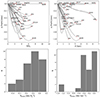 |
Fig. 1. Radial metallicity profiles and metallicity gradients calculated for our sample of dwarf galaxies. Top: smoothed [Fe/H] profiles as a function of SMA radius as obtained from the GPR fitting method in units of the 2D half-light radius (left) and as a function of physical radius (right). The radial metallicity profiles have been normalised to their value at R = 0. Dwarf galaxy names are as in Table 1. Bottom: distributions of the calculated metallicity gradients in the same units as in the top panels; bin widths were obtained following the Freedman-Diaconis normal reference rule. |
As shown in Fig. 1, the profiles are either flat or decline with radius; a slight increase is often seen in the outskirts, but when the individual [Fe/H] as a function of radius is compared with the GPR profile, this increase appears to be due to over-fitting of these sparse outer bins and can therefore be neglected. Therefore, the galaxies in our sample show either no metallicity gradients or negative metallicity gradients, out to the coverage of the spectroscopic datasets. We refer to Figs. A.1–A.5 for a detailed view of the individual [Fe/H] datasets and the corresponding GPR fits.
We proceeded to quantify the strength of the [Fe/H] gradient. Because we are interested in the average slope of the radial metallicity profile, we performed a linear fit on the smooth function returned by the GPR between R = 0 and the projected SMA radius where the GPR curve presents a minimum (or at the last measured point, in absence of a minimum). This was motivated by the fact that the GPR curves are mostly linear or parabolic in the considered range. The gradient value is therefore the slope of the linear fit. Its associated error is the error obtained on the slope parameter by performing a linear fit to the data instead1.
Because we compared galaxies of different sizes, we determined the gradient both in units of the 2D SMA half-light radius, ∇[Fe/H](R/Re), and in units of physical radius, ∇[Fe/H](R). The results are given in Table 2, and their distributions are shown in the bottom panels of Fig. 1, where the number of bins (and therefore their widths) was set following the Freedman-Diaconis normal reference rule2.
Adopted and derived parameters.
The distribution of gradient values covers the interval from ∼−0.4 dex  to ∼0 dex
  , or ∼−1.3 dex kpc−1 to ∼0 dex kpc−1, with the majority of the systems found in the range ∼−0.2 dex
  to ∼0 dex
  , and ∼−0.5 dex kpc−1 to ∼0 dex kpc−1. Median values are ∇[Fe/H](R/Re)∼ − 0.1 dex
  and ∇[Fe/H](R)∼ − 0.25 dex kpc−1, with a median absolute deviation scatter of 0.14 dex
  and 0.24 dex
  , respectively.
The different sample sizes, spatial coverages, and radial trends turn into rather different uncertainties in the recovered gradients. The ∇[Fe/H](R/Re) measures have associated errors ranging from 0.006 dex  to 0.14 dex
  , while for ∇[Fe/H](R), the errors reach from 0.004 dex kpc−1 to 0.43 dex kpc−1. In particular, the large ∇[Fe/H](R/Re) uncertainty for NGC 6822, despite its high number of individual metallicity measurements, arises because the spectroscopic sample covers an area just inside its half-light radius, even though this spans more than 10′ across the sky.
Finally, to verify that our method of deriving metallicity gradients does not rely too much on the position of the minimum on the GPR curves, we compared our results with those obtained by calculating the gradient as the difference in metallicity between the centre and 2 × Re of the GPR curves. We found a good general agreement (see Fig. B.3 in Appendix B). The only outlier (i.e. at > 3-σ) is Sculptor, which was found to have a steeper gradient. Even if we were to assume this value, our conclusions would still remain unchanged.
4. Comparison of the metallicity gradients
We report how the metallicity gradient strengths compare to different galaxy properties (host distance, stellar mass, and star formation timescales) for the considered sample of LG dwarf galaxies. Similarly, we analyse the role of angular momentum and past mergers.
4.1. Trends with environment and morphological type
In order to examine the role of the environment, we searched for possible trends with distance to the nearest large spiral. As shown in Fig. 2, neither satellite dwarfs nor isolated systems show on visual inspection any particular differences depending on their distance from the MW or M31 centres (see values in Table 2). We obtained distances using the distance modules from Battaglia et al. (2022) and the references in Table A.1. For M31, we assumed the coordinates and heliocentric distance from Conn et al. (2012), and for the MW, we assumed a heliocentric distance of 8.122 kpc (GRAVITY Collaboration 2018) and the Galactic centre coordinates from Reid & Brunthaler (2004).
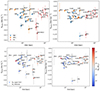 |
Fig. 2. Distribution of metallicity gradients as a function of distance from the nearest large LG spiral. Top: satellites of the Milky Way, M31, and the isolated systems are marked as blue circles, orange squares, and red triangles, respectively. Dwarf galaxies that might have experienced a past merger event are marked with an open circle. Bottom: same as above, but with data colour-coded according to their HI content; circles mark a full detection, and squares mark the 5-σ upper limit (data from Putman et al. 2021, and references therein). On the y-axes, the left panels show the metallicity gradients in units of the 2D SMA half-light radius, and in the right panels, they are in units of the physical radius. |
In general, the distribution of the metallicity gradients (either as ∇[Fe/H](R/Re) or ∇[Fe/H](R)) of satellite systems apparently has a slightly larger scatter than that of isolated dwarfs. However, when they are compared using the Kolmogorov-Smirnov and Anderson-Darling statistical tests (using scipy.stats functions ks_2samp and anderson_ksamp), the distributions do not show a statistically significant difference.
We note that the systems with the strongest ∇[Fe/H](R/Re) (i.e. ≲−0.25 dex  ) are present both among the isolated dwarf galaxies and among the satellites; removing them from our analysis does not change our conclusions. We also point out that the majority of these systems may have experienced a merger event in their past (see e.g., Amorisco et al. 2014; Kacharov et al. 2017; Cicuéndez & Battaglia 2018, for the cases of And II, Phoenix, and Sextans, respectively; but also Battaglia et al. 2006; Amorisco & Evans 2012; de Boer et al. 2012; del Pino et al. 2015; Leung et al. 2020, for the case of Fornax; and de Blok & Walter 2000, 2006; Demers et al. 2006; Battinelli et al. 2006; Hwang et al. 2014, but also Zhang et al. 2021, for the case of NGC 6822), and potentially, mergers may play a role in driving the formation of strong gradients (Benítez-Llambay et al. 2016). We refer to Sect. 4.5 for more details about this aspect.
We further searched for differences between the metallicity gradients by grouping our sample according to the galaxy HI-gas content (see Fig. 2, bottom panels; MHI data from Putman et al. 2021). In particular, we searched for statistical differences between the gas-poor (i.e. dSph, cE/dE; see Table 1) and the gas-rich systems (the dIrr and dTr), but found none. This is in contrast to the results reported by Leaman et al. (2013), who found a dichotomy between the dSphs and dIrrs, with the former showing a radially decreasing metallicity profile, while the latter had a flat profile. We attribute this discrepancy mainly to the limited sample of dwarf galaxies they analysed, which we tripled in number here.
These results indicate a limited role of the prolonged environmental interaction between a satellite and its host galaxy as the main actor in the formation of strong radial metallicity gradients in LG dwarf galaxies. Whether tidal and ram-pressure stripping eventually have a role in shaping metallicity gradients could depend on several factors, such as the internal properties and orbital history of the satellite, the build-up stage of the host, and whether the satellite fell into the host potential before or after its star formation had shut down (based on Mayer et al. 2007; Sales et al. 2010; Hausammann et al. 2019; Di Cintio et al. 2021). Although any process in general related to the mixing of stellar orbits might weaken an existing gradient (e.g., Sales et al. 2010), depending on the orbit, an encounter with a host could trigger central star formation in a gas-containing dwarf galaxy, leading instead to a strengthening of its metallicity gradient (e.g., Hausammann et al. 2019; Di Cintio et al. 2021; see also discussion in Koleva et al. 2011). Overall, the environment apparently has the potential to increase the scatter in the distribution of metallicity gradients in satellites, an indication of which is shown in Fig. 2. The statistics are currently such that we cannot firmly confirm this conclusion, however.
We further searched for possible correlations between the metallicity gradients of the MW satellites and their quenching timescale (i.e. the time spent by a dwarf galaxy to form 90% of its stars after its first infall into the MW potential, as calculated by Fillingham et al. 2019 and Miyoshi & Chiba 2020 using Gaia-DR2 proper motions), but found none. We also examined the orbital parameters (i.e. eccentricity, pericentric distance, period, and time since the last pericentric passage) provided by Battaglia et al. (2022) considering different MW-potentials, but our sample is too small (12 dwarf galaxies) to reach definitive conclusions. For reference, we show our results in Appendix C.
4.2. Trends in galaxy luminosity
Figure 3 shows an overview of the strength of the metallicity gradient as a function of the galaxy luminosity in the V band (see values in Table 2). The distribution of ∇[Fe/H](R/Re) displays a large scatter (left panel); on the other hand, ∇[Fe/H](R) weakly indicates a relation with LV (right panel) as shown by the linear fit (with a slope m = 0.05 ± 0.02) and the 95% confidence interval. This seems to be a manifestation of the fact that more luminous galaxies are in general larger than fainter ones (e.g., Tolstoy et al. 2009), as is reflected by the fact that the relation weakens significantly for ∇[Fe/H](R/Re), that is, when normalising for the half-light radius, with the confidence interval being consistent with no linear relation (m = 0.01 ± 0.01).
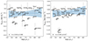 |
Fig. 3. Distribution of metallicity gradients as a function of the galaxy luminosity in V band with the respective uncertainties. The dashed blue lines represent the linear LSQ fit to the data and the blue shaded areas show the 95% confidence interval. In the legend boxes we report the slope value from the LSQ fits. On the y-axes, the left panel shows the metallicity gradients in units of the 2D SMA half-light radius, while on the right panel, they are in units of the physical radius. Dwarf galaxies that may have experienced a past merger event are marked with an open circle. |
We reached the same conclusion by replacing LV with the average metallicity ⟨[Fe/H]⟩, recovering a correlation with ∇[Fe/H](R) due to the luminosity-metallicity relation (e.g., Kirby et al. 2013b), and with the velocity dispersion σv , which is a proxy of the dynamical mass inside the half-light radius M1/2 (Walker et al. 2009; Wolf et al. 2010). We are aware that σv could be a biased mass-indicator when significant internal rotation is present (i.e. Vrot/σv ≳ 0.5). Accounting for this effect (see e.g., Kirby et al. 2014), however, would have a negligible effect on the relation between ∇[Fe/H](R) and M1/2.
To make a qualitative comparison, stellar metallicity gradients have also been detected in early- and late-type field galaxies (with 8.0 < log(M*/M⊙)< 11.5 and distances z ≲ 0.03). Only the former show no clear correlation between ∇[Fe/H](R/Re) and their stellar masses (see e.g., Koleva et al. 2011; Goddard et al. 2017).
On the other hand, zoom-in hydrodynamic simulations of isolated dwarf galaxies are also inconclusive about a correlation between ∇[Fe/H](R/Re) and stellar mass. Schroyen et al. (2013) and Revaz & Jablonka (2018, hereafter RJ18) found that additional factors could have an impact on the formation of metallicity gradients, for example their SFH and the presence of internal rotation. The absence of a correlation with stellar mass, average metallicity, but also with stellar rotation (although they had a few systems with Vrot/σv > 0.5) was instead reported by Mercado et al. (2021, see their Fig. A2), who conversely found a tight correlation with the median stellar age of their simulated systems (see Sects. 4.3, 4.4, and 5).
4.3. Correlation with star formation timescales?
To explore possible relations with star formation timescales, we considered the t50 and t90 quantities that indicate the look-back time at which the cumulative stellar mass inferred by the measured SFH reaches 50% and 90% of its current total value, respectively (see values in Table 2). We used the compilations of Weisz et al. (2014, 2015), except for the dwarfs analysed by Bettinelli et al. (2018) and Albers et al. (2019).
Figure 4 shows that no clear correlations emerge when metallicity gradients are plotted per unit of the 2D half-light radius, either as a function of log(t50) (top left) or log(t90) (bottom left). When we instead consider metallicity gradients per units of physical radius (right panels), a stronger relation appears with both t50 and t90. In particular, for the latter quantity, we obtain a significant slope value of m = −0.29 ± 0.11 from the linear LSQ fit. The correlations observed for ∇[Fe/H](R) are again a manifestation of the scaling relations among dwarf galaxies, as seen in the previous section. In this case, they are in large part a consequence of the fact that fainter dwarf galaxies (which have smaller Re) show shorter SFHs on average than brighter dwarf galaxies (which have larger Re; see e.g., Weisz et al. 2015). This is reflected by the weak trends observed for ∇[Fe/H](R/Re) (i.e. normalising for Re) that are consistent with no linear relation within the confidence intervals. The same conclusions are reached by expressing t50 and t90 values on a linear instead of a logarithmic scale. It is worth noting that some of these measures have large associated errors that could smear any possible correlation, so it would be particularly useful in the future to have access to SFHs that are both homogeneous and more accurate and precise than currently available compilations.
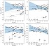 |
Fig. 4. Distribution of metallicity gradients as a function of the t50 (top panels) and t90 (bottom panels) for our sample of dwarf galaxies. The dashed blue lines represent the LSQ fit to the data and the blue shaded areas show the associated 95% confidence interval. On the y-axes, we plot the metallicity gradients in units of the 2D SMA half-light radius (left panels) and in units of the physical radius (right panels). In the legend boxes we report the slope value from the LSQ fits. Dwarf galaxies that may have experienced a past merger event are marked with an open circle. |
An important result of this analysis is the lack of a clear and strong correlation between ∇[Fe/H](R/Re) and t50, in contrast with the results obtained by Mercado et al. (2021). Analysing a set of simulated dwarf galaxies with stellar masses comparable to those of our dataset, Mercado et al. (2021) found a linear relation between the median age and the metallicity gradient of their simulated systems. This result was supported by a restricted sample of ten LG dwarf galaxies following a similar relation. As discussed in Sect. 5.1, but as also visible from Fig. 4 (upper left panel), when the observed sample size is increased, the clear correlation found by Mercado et al. (2021) practically disappears.
The link between the length of the star formation period and the emergence of metallicity gradients in dwarf galaxies, on the other hand, has been explored by RJ18. They analysed a different set of simulated dwarf galaxies. We refer to Sects. 5.1 and 5.2 for a detailed comparison between these sets of simulations and our analysis.
4.4. Role of angular momentum
Cosmological zoom-in simulations have highlighted the role played by angular momentum in preventing a radial metallicity profile in dwarf galaxies. Schroyen et al. (2013) and RJ18 have shown that a significant angular momentum may produce a centrifugal barrier that prevents the gaseous component from flowing towards the centre of the galaxy, thus preventing star formation from becoming more spatially concentrated and a metallicity gradient from forming. In particular, RJ18 found that internal rotation has a significant impact in preventing the formation of a radial metallicity profile in the highest-mass systems of their sample (i.e. with M* ≳ 108 M⊙), which are also those with the longest SFHs.
In our sample, significant stellar rotation (i.e. with 0.5 ≲ Vrot/σv ≲ 2.0) has been detected in the SMC (De Leo et al. 2020), the dEs (Geha et al. 2006, 2010), WLM (Leaman et al. 2012), IC 1613 (Wheeler et al. 2017; Taibi et al. in prep.), NGC 6822 (Demers et al. 2006; Wheeler et al. 2017), and at lower masses in Aquarius (Hermosa Muñoz et al. 2020), Pegasus (Kirby et al. 2014), and probably Carina (Martínez-García et al. 2021). It was reported as prolate rotation in And II (Ho et al. 2012) and Phoenix (Kacharov et al. 2017).We do not include in this list M32 and Antlia II, for which clear signs of internal stellar rotation have been observed, but that may have been caused by tidal perturbations from their hosts (Howley et al. 2013; Ji et al. 2021). We also note that the Carina Vrot/σv value reported by Martínez-García et al. (2021) is significant at the 2-σ level.
To better compare the properties of the rotating systems with the rest of the sample, we show in Fig. 5 the observed stellar luminosity of our systems compared to their SFH duration (i.e. their log(t90/yr)), with marker sizes and colours proportional to their ∇[Fe/H](R/Re); rotating dwarfs are highlighted with a different symbol. Because the SMC, VV 124, Antlia II, and Crater II have no calculated t90 from the literature, we gave them fiducial values based on the length of their SFH (Jacobs et al. 2011; Rubele et al. 2018; Walker et al. 2019; Ji et al. 2021).
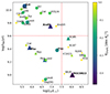 |
Fig. 5. Luminosity vs. t90 for our sample of dwarf galaxies. Systems that shows significant stellar rotation are marked with triangles, all the others are shown with circles; merger candidates are highlighted with bold text, and the colour-coding and marker sizes are according to the value of their metallicity gradients ∇[Fe/H](R/Re). Dashed red lines identify the sub-regions considered in Sect. 4.4. |
We observe that 7 out of 12 of the rotating systems have high stellar masses and extended SFHs (i.e. log(LV/L⊙)> 7.5 and log(t90/yr)< 9.6). Four of them show ∇[Fe/H](R/Re) consistent with 0 within the 1-σ error. On the other hand, of the remaining rotating systems with lower stellar masses, just one shows a flat [Fe/H] profile within the errors (i.e. Carina, which has an uncertain Vrot/σv detection, however). Thus, although milder gradients along with significant stellar rotation are likely to be observed among massive dwarf galaxies with an extended SFH, the same does not necessarily hold at low stellar masses.
It is interesting to further explore the properties of the low-mass systems. Those that have extended SFHs (i.e. log(t90/yr)< 9.6) are characterised by strong rotating systems and have ∇[Fe/H](R/Re) values with a median and scatter of −0.12 dex  and 0.14 dex
  , respectively.
Fainter systems that have formed stars for a shorter period (i.e. having log(LV/L⊙)< 7.5 and log(t90/yr)> 9.6) and that in general are not rotating (e.g., Wheeler et al. 2017) show negative gradients with a similar median of −0.11 dex  , but a smaller scatter of 0.06 dex
  . It is difficult, however, to ascertain whether SFH and angular momentum play a role in driving the scatter of ∇[Fe/H](R/Re) values between the two sub-samples of low-mass systems (apart from the presence of peculiar systems, such as prolate rotators) mainly due to their limited sizes.
4.5. Role of mergers
In our sample, several systems may have experienced a dwarf-dwarf merger in their past, namely Andromeda II (Amorisco et al. 2014; Lokas et al. 2014; del Pino et al. 2015), Phoenix (Kacharov et al. 2017), Sextans (Cicuéndez & Battaglia 2018), Fornax (Battaglia et al. 2006; Amorisco & Evans 2012; de Boer et al. 2012; del Pino et al. 2015; Leung et al. 2020; Pace et al. 2021), and NGC 6822 (de Blok & Walter 2000, 2006; Demers et al. 2006; Battinelli et al. 2006; Hwang et al. 2014; Zhang et al. 2021). Evidence supporting a past (z ≲ 1) major merger in these dwarf galaxies includes stellar substructures (including shell- or stream-like features), and peculiar structural or kinematic properties (e.g., prolate rotation).
We find in our analysis that the merger candidates are all characterised by a strong metallicity gradient. The ∇[Fe/H](R/Re) values are narrowly distributed around −0.35 dex  (Figs. 2–5).
Simulations have shown that these strong gradients can be the result of a past merger event. Benítez-Llambay et al. (2016), analysing a set of dwarf galaxies from the CLUES simulation, reported two main conditions for steep gradients to occur: a dwarf-dwarf merger must take place to disperse the old, metal-poor stellar components formed before the event, and in situ and centrally concentrated star formation must follow the subsequent accretion of residual gas. Cardona-Barrero et al. (2021), analysing the set of simulations of RJ18, have also shown that a major merger can cause the production of a prolate stellar rotation together with a strong metallicity gradient, both features observed in And II and Phoenix (Ho et al. 2012; Kacharov et al. 2017).
According to Deason et al. (2014), the majority of dwarf-dwarf mergers have occurred at high-z, with an expected 10% (15−20%) of dwarf satellite (isolated) systems with M* ≳ 106 M⊙ having experienced a major merger since z = 1. Specifically for the LG, they expect this to be the case for ∼1−3 (∼2−5) MW or M31 satellite dwarfs (isolated). These numbers agree well with those of our merger candidates, considering that they cover the same stellar mass range (where our full sample is almost complete, especially considering MW satellites and isolated systems).
If we were to exclude the merger candidates from the full distribution of metallicity gradients, the median and scatter of the sample would reduce to −0.08 dex  and 0.11 dex
  , respectively. The intrinsic scatter (i.e. taking into account measurement errors on the gradient values) about the median of this distribution would be only 0.05 dex
  . This result indicates that the values of ∇[Fe/H](R/Re), when merger candidates are excluded, are remarkably similar to each other despite the large differences in the properties of the analysed systems, which we recall span three orders of magnitude in luminosity, have formed stars on various timescales, and live in different environments. This may also indicate that the formation of mild metallicity gradients is intrinsic to the evolution of dwarf galaxies.
5. Comparison with simulations
Several works in the literature have followed the chemical evolution of dwarf galaxies in cosmological zoom-in simulations, exploring the interplay between gravity, angular momentum, and stellar feedback. The result of which may eventually lead or may not lead to the formation of metallicity gradients.
In this section, we examine in more detail whether the predictions of these simulations agree with our observations. In particular, we compare our results with those of Mercado et al. (2021), and we apply the same method used for the observed sample to analyse the systems simulated by Revaz & Jablonka (2018) and those presented in Bellovary et al. (2019), Akins et al. (2021) and Munshi et al. (2021). The considered simulations cover a stellar mass range similar to that of the observations (105 ≲ M*/M⊙ ≲ 109), but were generated using distinct hydrodynamic codes and different stellar feedback recipes.
5.1. Comparison with Mercado et al. (2021)
Mercado et al. (2021, hereafter M21), analysing a set of 26 isolated dwarf galaxies from the FIRE-2 simulation with stellar masses in the range 105.5 < M*/M⊙ < 108.3, found a significant linear relation between ∇[Fe/H](R/Re) and t50. The authors explain this correlation as due to the combined effect of two different mechanisms. Repeated episodes of stellar feedback ‘puff up’ the spatial distribution of stars: because older, more metal-poor populations experience more of these cycles than younger and metal-richer populations, the puffing-up will be stronger in the former than in the latter, creating a metallicity gradient. Whether this gradient remains strong or weakens then depends on the extent of the late star-forming spatial region: in galaxies that experience late gas accretion, this (recycled or metal-enriched) gas tends to be deposited at large radii, feeding the formation of metal-richer stars in the outskirts, and thus weakening the metallicity gradient. Although with a shallower slope, the authors obtained a similar dependence for a sample of ten LG dwarf galaxies, both isolated and satellites, based on t50 and ∇[Fe/H](R/Re) derived from SFHs and radial metallicity profiles, respectively, from spectroscopic observations available in the literature.
For the sake of comparison, Fig. 6 (left) shows the relation between the strength of the metallicity gradients with respect to t50 obtained by M21 for simulated galaxies (dotted black line) compared to the observed relation they obtained for their selected sub-sample of LG dwarf galaxies (orange squares and dashed line). We overplot our determination of the [Fe/H] gradient for the same sub-sample (blue circles and dashed line). In order to be consistent, we calculated the metallicity gradients as in M21, that is, using the 2D circular radii3 and limiting the analysis to twice the 2D projected geometric half-light radius. Values for our galaxy sample are reported in Table A.2. We also report in the figure the same t50 values as were tabulated by M21.
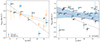 |
Fig. 6. Comparison with Mercado et al. (2021). Left: metallicity gradients as a function of t50 obtained by Mercado et al. (2021) for a sample of LG dwarf galaxies marked by orange squares with error bars, compared with our determinations for the same sample obtained following the Mercado et al. (2021) criteria (i.e. assuming circular radii and with gradients calculated within 2 × Re, circ) marked by blue circles with error bars. The dashed orange and blue lines are the linear LSQ fits to the described samples, respectively, while the dotted black line (in both panels) is the linear relation found by Mercado et al. (2021) for their set of simulated systems. Right: metallicity gradients obtained again following the Mercado et al. (2021) criteria, but for the full sample of galaxies analysed in this work as a function of their t50 adopted from Weisz et al. (2014), Bettinelli et al. (2018) and Albers et al. (2019); the dashed blue line and shaded area are the linear LSQ fit and the associated 95% confidence interval of the sample, respectively. As reference, red circles mark the sub-sample considered by Mercado et al. (2021). The dashed red line is the linear fit to it. |
This figure shows that the different spectroscopic samples and/or method we use cause differences in the values of the gradient strength of the individual galaxies, but overall, the trend with t50 remains, even though our relation is slightly shallower that theirs (m = −0.013 ± 0.005). Our calculated values further highlight the discrepancy with the theoretical trend (dashed black line) obtained by M21 from their simulated sample (mM21 = −0.036 ± 0.005).
In Fig. 6 (right) we instead show the metallicity gradients again assuming 2D circular radii, but this time, for our full sample of galaxies as a function of their t50 values listed in Table 2 (see Sect. 4.3 for further details). Increasing the sample size further flattens the relation with t50 (m = −0.009 ± 0.006), with the 95% confidence interval fully consistent with there being no relation between the two quantities. The sub-sample of LG dwarf galaxies selected by M21 are marked in red; they show a linear decreasing trend comparable to the one obtained in the left panel, despite the slight difference in the t50 values considered.
The observations, therefore, do not seem to back up the theoretical prediction of a clear relation between strength of the metallicity gradient and t50. This might be a consequence of the observed uncertainties related to the determination of t50 smudging the relation, or simply indicate a lower impact of stellar feedback in the evolution of LG dwarf galaxies with respect to that involved in the FIRE-2 simulations.
5.2. Comparison with Revaz & Jablonka (2018)
The link between the full length of the star formation period and metallicity gradients in dwarf galaxies has been explored by RJ18, who analysed a set of cosmological zoom-in simulations of 27 isolated dwarf galaxies with stellar masses between 105.5 − 108.75 M⊙. They showed that as long as star formation is active, metallicity gradients build up gradually because the gas reservoir shrinks towards the galaxy centre. In fainter systems (i.e. with M* ≤ 106 M⊙), star formation is soon quenched by the UV background heating, and thus gradients tend to be marginal. Similarly, at higher masses, a significant angular momentum counteracts their sustained SFH, producing flatter metallicity profiles. A major merger, however, could lead to the formation of a relatively strong and long-lasting gradient at any mass (see also Benítez-Llambay et al. 2016; Cardona-Barrero et al. 2021). We note that the RJ18 simulations use a different star formation recipe that leads to a lower impact of stellar feedback than the FIRE-2 simulations analysed by M21.
We have analysed here the simulated systems presented in RJ18 by applying the same method as we used for our observed dataset in order to calculate their metallicity gradients and perform a direct comparison with the LG systems. We adopted a fiducial [Fe/H] error of 0.2 dex for the stellar particles in the simulations, which is a typical observational uncertainty.
As shown in Fig. 7, the scenario described by RJ18 produces a shape resembling a U in the diagrams where the ∇[Fe/H](R/Re) is seen against the stellar mass or the t90. The strongest gradients are observed for systems at intermediate masses (i.e. log(M*/M⊙)∼7.0) with extended SFHs; systems at the high-mass end, characterised by a continuous and sustained SFH, have marginal gradients due to their high angular momentum; at the low-mass end instead, where the SFH is soon quenched, gradients show a large scatter.
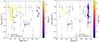 |
Fig. 7. Distribution of the metallicity gradients calculated for the simulated systems presented in Revaz & Jablonka (2018), on the left panel as a function of their stellar mass and color-coded according to their t90, while inverting these two variables in the right panel. Numbers identify the individual halos mentioned in the main text, while the gradient values for the Local Group dwarf galaxies presented in this work are shown as grey circles with their associated error bars. We have assumed in this case a stellar mass-to-light ratio of one. |
The simulations cover a similar range of ∇[Fe/H](R/Re) values as the observed galaxies, with a median and scatter of −0.09 dex  and 0.10 dex
  , respectively. These values are comparable to the observed ones, excluding the merger candidates, as shown in Fig. 8, where we performed a kernel density estimation (assuming in all cases a Gaussian kernel of bandwidth 0.04 dex
  , i.e. comparable to the average error of the metallicity gradients). To compare the different distributions, we used the PYTHON package KernelDensity in scikit-learn (Pedregosa et al. 2011).
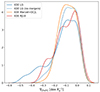 |
Fig. 8. Kernel density estimation of the metallicity gradient distribution for the LG sample (with and without merger candidates as solid and dashed blue lines, respectively), compared with the simulated sets of Revaz & Jablonka (2018, red line) and the DCJL plus MARVEL ones (orange line) analysed in Sects. 5.2 and 5.3, respectively. We assumed in all cases a Gaussian kernel with a bandwidth of 0.04 dex |

The simulated systems do not show ∇[Fe/H](R/Re) values that are in absolute terms as extreme as the observational ones, although when the error bars are taken into account, these may be plausible. On the other hand, two of the strongest gradients in the simulations (i.e. for h061 and h048) are for systems that experienced a major merger at ∼6 Gyr (see also Cardona-Barrero et al. 2021). We note that the strong gradient observed for h039 is instead caused by its large half-light radius, artificially enhanced due to the presence of small ultra-faint satellites orbiting it, with some of them in a process of being merged or destroyed at z = 0.
Despite the general agreement, we do not recover a strong dependence between the values of ∇[Fe/H](R/Re) and the stellar mass or SFH of the observed systems as for the simulated ones. In particular, we observe a larger scatter of observed systems at log(M*/M⊙)∼7.0 and log(t90/yr)∼9.5, where the formation of strong gradients should be favoured by their extended SFH. This may be due to the limited sample of simulated galaxies analysed by RJ18, which does not include analogues of observed dwarf galaxies such as Carina, Leo I, and Fornax, but also Aquarius and Leo A, characterised by a significant fraction of intermediate age stars (e.g., Gallart et al. 1999; de Boer et al. 2012, 2014; Cole et al. 2014; Ruiz-Lara et al. 2021). These limitations could also be due to the specific galaxy formation model implemented in RJ18, in particular regarding the impact of the UV-background heating and/or the efficiency of hydrogen self-shielding. However, as shown in RJ18, their simulated galaxies are able to reproduce over several orders of magnitudes the observed properties of LG systems in terms of LV, σv, Re, and MHI. Therefore, it is difficult to attribute the lack of intermediate-mass dwarf galaxies with an extended SFH in the RJ18 sample to a limitation of their model or to a simple lack of sufficient statistics.
We recall that RJ18 simulations follow the evolution of dwarf galaxies in isolation. The influence of an MW host on the same set was explored by Hausammann et al. (2019), who found that indeed ram-pressure and tidal interactions could help star formation last longer, with a possible impact on the formation of metallicity gradients. However, this would require very specific conditions (a very late entry with a small pericenter in the MW-potential, or a very early accretion) which seems to limit the actual role of a MW-like host. We have shown in Sect. 4.1 that we find no significant differences between the metallicity gradient properties of satellite and isolated systems.
5.3. Comparison with DCJL and MARVEL sets
We further analysed a sample of dwarf galaxies selected from two sets of zoom-in cosmological simulations: the near-mint DC Justice League (DCJL) presented in Bellovary et al. (2019) and Akins et al. (2021), and the MARVEL-ous Dwarfs (MARVEL) from Munshi et al. (2021). The DCJL set consists of ∼100 dwarf galaxies from four MW-like environments (namely Sandra, Ruth, Sonia, and Elena) that mimic the MW in terms of host halo-mass but with different formation histories. The MARVEL set instead is formed by ∼50 field dwarfs (some of which are satellites of dwarf galaxies) from four low-density environments (called CptMarvel, Elektra, Rogue, and Storm). Both sets of simulations were run using the same code and underlying physics.
The analysed systems cover a similar range of stellar masses as the RJ18 and M21 simulations, which, however, implemented different stellar feedback recipes with, simplifying, the DCJL and MARVEL sets halfway between the RJ18 set, characterised by low feedback, and M21 (see Iyer et al. 2020, for a comparison between the burstiness of the DCJL/MARVEL and FIRE-2 sets). We refer to Bellovary et al. (2019), Akins et al. (2021) and Munshi et al. (2021) for further details about the DCJL and MARVEL simulations.
The analysis of these simulated systems was conducted applying the same method as we developed for our observed dataset to calculate their metallicity gradients; this method was also used for the RJ18 set. The individual metallicity values initially had no associated uncertainties, hence we adopted a fiducial [Fe/H] error of 0.2 dex for each stellar particle. Our results show that the obtained ∇[Fe/H](R/Re) in all cases range between −0.25 dex  and 0 dex
  , with medians and scatter values of about −0.10 dex
  and 0.09 dex
  (see Figs. 8 and 9). We also find that both DCJL and MARVEL systems show similar ∇[Fe/H](R/Re) distributions, which suggests that the environment plays a limited role in these simulations in driving the scatter of metallicity gradients. The obtained results again agree well with our observations, except for the steepest gradients we observed, which have no match in these simulations. In addition, similar to our observations, the simulated systems show no clear correlations between their ∇[Fe/H](R/Re) and the stellar mass or with their t50 or t90 (see again Fig. 9). In a forthcoming paper, we will provide details on the chemical and star formation history of these simulated systems, together with an analysis of their past merger history and a thorough comparison with other sets of simulations carried out with different initial conditions and stellar feedback recipes (e.g., the aforementioned RJ18 simulations).
 |
Fig. 9. Distribution of the metallicity gradients calculated for the simulated systems of both the DCJL and MARVEL sets as a function of their stellar mass colour-coded according to their t90 (top left) and t50 (top right), and as a function of t90 (bottom left) and t50 (bottom right) in both cases colour-coded according to their stellar mass. We also show the gradient values for the LG dwarf galaxies presented in this work, shown as grey circles with their associated error bars. We have assumed a stellar mass-to-light ratio of one in this case. |
6. Summary and conclusions
We conducted a homogeneous search and measurement of stellar metallicity gradients in LG dwarf galaxies. We used publicly available spectroscopic catalogues of red giant stars in 30 systems, either isolated galaxies or satellites of the Milky Way and M31. This is the largest compilation of this type to date.
We analysed the radial variation of the metallicity [Fe/H] values using a Gaussian process regression analysis. From the resulting profiles, we determined a value for the metallicity gradient, both in units of the physical radius in kpc, ∇[Fe/H](R), and in units of the 2D SMA half-light radius, ∇[Fe/H](R/Re). We find that the majority of systems we analysed show negative gradients, with median values ∇[Fe/H](R/Re)∼ − 0.1 dex  , and ∇[Fe/H](R)∼ − 0.25 dex kpc−1.
Our systems show no correlation between their gradients and their morphological types (or internal gas content) or with the distance from the nearest host galaxy (i.e. the MW or M31). These results indicate that the environment as the main actor in the formation of strong radial metallicity gradients in LG dwarf galaxies plays a limited role. An important fact here is the presence of negative gradients in the isolated systems.
We find mild correlations between ∇[Fe/H](R) and the stellar luminosity of our systems, as well as with their t50 and t90 values (i.e. the look-back times at which the cumulative stellar mass inferred by the SFH reaches 50% and 90% of its total value, respectively), as a result of the scaling relations among LG systems (i.e. stellar mass-size, stellar mass-metallicity, and stellar mass-SFH relations). No clear correlations are found with the same parameters for ∇[Fe/H](R/Re).
In particular, we inspected the dependence of ∇[Fe/H](R/Re) on t50, which was found by Mercado et al. (2021) to exhibit a strong anti-correlation with the gradient strength in their simulated dwarfs. While we recovered the shallow dependence that they found for a sub-sample of ten LG dwarf galaxies, when we considered the full sample we analysed, the trend between the strength of ∇[Fe/H](R/Re) and t50 is consistent with no correlation between the two quantities.
We also searched for differences in the values of ∇[Fe/H](R/Re) of systems with significant stellar rotation. Simulations have shown that a high angular momentum could prevent the formation of strong gradients, particularly at higher masses (Schroyen et al. 2013; Revaz & Jablonka 2018). Dwarf galaxies with LV > 107.5 L⊙, characterised by an extended SFH and significant stellar rotation, include some systems with flat metallicity gradients. However, when the remaining rotating systems are taken into account, a high angular momentum does not necessarily imply a flat gradient.
The strongest gradients in our sample, ∇[Fe/H](R/Re)≲ − 0.25 dex  , are observed in And II, Phoenix, Sextans, Fornax, and NGC 6822. These are all systems that have been proposed as likely to have experienced a past merger event in the literature, given the chemo-kinematic properties of their stellar component. Simulations have shown that a dwarf-dwarf merger event followed by a re-ignition of star formation activity in the galaxy centre would indeed produce strong metallicity gradients (Benítez-Llambay et al. 2016; Cardona-Barrero et al. 2021).
When the merger candidates are excluded from the full distribution of metallicity gradients, the median ∇[Fe/H](R/Re) reduces to −0.08 dex  with an associated intrinsic scatter of only 0.05 dex
  . This result indicates that metallicity gradients of LG dwarf galaxies are remarkably self-similar despite the large differences in their observed properties (i.e. in terms of stellar mass, star formation history, and environment).
We complemented our study with the analysis of simulated dwarf galaxies from the literature by applying the same method we used for the observed sample to calculate their metallicity gradients. In particular, we examined the sample of Revaz & Jablonka (2018) (∼30, isolated dwarf galaxies) and recovered their previous results. We found that the average and scatter of their ∇[Fe/H](R/Re) values agree well with those of the observations. However, differently from their work, we did not recover any correlation between ∇[Fe/H](R/Re) and the luminosity and SFH of the observed systems. We note that our sample contains low-mass systems with an extended SFH, which have no counterparts in their simulations.
Similarly, we analysed a sample of simulated dwarf galaxies (∼150, either central or satellites of MW-like hosts) selected from two sets of cosmological simulations: DCJL (Bellovary et al. 2019; Akins et al. 2021), and MARVEL (Munshi et al. 2021). We obtain comparable ∇[Fe/H](R/Re) distributions between the different simulated samples, whose values again agreed well with those of the observed systems after we excluded the steepest gradients that have no match in the simulations. Similarly to the observations, we further find that the simulated systems show no clear correlation between their gradients and stellar mass or with t50 or t90.
In general, the interplay between the several internal factors that could led to the formation of metallicity gradients appears to be more complex than what is shown by the simulations with which we have compared our results. The role of the environment, on the other hand, seems limited, although we cannot exclude that effects such as tidal and ram-pressure stripping may have an impact in increasing the scatter of metallicity gradient values among the satellite systems.
The study of radial metallicity gradients in LG dwarf galaxies will benefit in the future from further investigations. From an observational point of view, it would be important to extend the surveyed area of some systems, in particular for NGC 6822. To confirm that its radial metallicity profile continues to be so steep even at larger radii would be of particular relevance in the context of the connection between strong gradients and major merger events.
On the other hand, in order to better understand the impact that star formation timescales have on the formation of metallicity gradients in dwarf galaxies, it would be useful to have measurements of their SFHs that are both homogeneous and more accurate and precise than those currently available. In this context, it would also be interesting to explore how the metallicity gradients compare to the radial age gradients that could be obtained from the analysis of individual stars.
Finally, we plan in the future to perform a thorough comparison between the sets of simulations considered in this work, which differ in their initial conditions, environment, and implemented stellar feedback recipes. We wish to provide the astronomical community with constraints on the processes that shape the formation and evolution of dwarf galaxies in the LG with our results.
Our method for deriving metallicity gradients is mostly equivalent to calculating the derivative of a GPR curve, which is differentiable, over the same interval and obtaining the average of this derivative. This gives us the average slope of the radial metallicity profile, similar to that obtained with the linear fit. The associated error is therefore the error obtained from a linear least-squares fit, assuming the error of the data is that of the GPR curve, which takes into account the uncertainties on the individual metallicity measurements together with the inherent dispersion of the data. This is again equivalent to obtaining the slope error of a least-squares linear fit to the raw data.
Acknowledgments
We wish to thank the anonymous referee for constructive comments that improved the manuscript. We thank M. Pawlowski, S. Cardona-Barrero, and A. Di Cintio for useful discussions and comments at different stages of this work. S.T. acknowledges funding of a Leibniz-Junior Research Group (PI: M. Pawlowski; project number J94/2020) via the Leibniz Competition. S.T. and G.B. acknowledge support from: the Agencia Estatal de Investigación del Ministerio de Ciencia e Innovación (AEI-MICIN) and the European Regional Development Fund (ERDF) under grant with reference AYA2017-89076-P, while the AEI-MICIN under grant with reference PID2020-118778GB-I00/10.13039/501100011033; G.B. acknowledge the AEI-MICIN under grant with reference CEX2019-000920-S. AMB and FDM acknowledge support from HST AR-13925 provided by NASA through a grant from the Space Telescope Science Institute, which is operated by the Association of Universities for Research in Astronomy, Incorporated, under NASA contract NAS5-26555. A.M.B. acknowledges support from HST AR-14281. A.M.B. and C.L.R. acknowledge support from NSF grant AST-1813871. Resources supporting this work were provided by the NASA High-End Computing (HEC) Program through the NASA Advanced Supercomputing (NAS) Division at Ames Research Center. This research has made use of NASA’s Astrophysics Data System, VizieR catalogue access tool (CDS, Strasbourg, France, DOI: 10.26093/cds/vizier), and extensive use of Python3.8 (Van Rossum & Drake 2009), including iPython (v8.3, Pérez & Granger 2007), Numpy (v1.21, Harris et al. 2020), Scipy (v1.7, Virtanen et al. 2020), Matplotlib (v3.5, Hunter 2007), Astropy (v5.0, Astropy Collaboration 2018) and Scikit-learn (v1.0, Pedregosa et al. 2011) packages.
References
- Akins, H. B., Christensen, C. R., Brooks, A. M., et al. 2021, ApJ, 909, 139 [NASA ADS] [CrossRef] [Google Scholar]
- Albers, S. M., Weisz, D. R., Cole, A. A., et al. 2019, MNRAS, 490, 5538 [NASA ADS] [CrossRef] [Google Scholar]
- Amorisco, N. C., & Evans, N. W. 2012, ApJ, 756, L2 [NASA ADS] [CrossRef] [Google Scholar]
- Amorisco, N. C., Evans, N. W., & van de Ven, G. 2014, Nature, 507, 335 [NASA ADS] [CrossRef] [Google Scholar]
- Astropy Collaboration (Price-Whelan, A. M., et al.) 2018, AJ, 156, 123 [Google Scholar]
- Battaglia, G., & Starkenburg, E. 2012, A&A, 539, A123 [NASA ADS] [CrossRef] [EDP Sciences] [Google Scholar]
- Battaglia, G., Tolstoy, E., Helmi, A., et al. 2006, A&A, 459, 423 [NASA ADS] [CrossRef] [EDP Sciences] [Google Scholar]
- Battaglia, G., Irwin, M., Tolstoy, E., et al. 2008, MNRAS, 383, 183 [NASA ADS] [CrossRef] [MathSciNet] [Google Scholar]
- Battaglia, G., Tolstoy, E., Helmi, A., et al. 2011, MNRAS, 411, 1013 [NASA ADS] [CrossRef] [Google Scholar]
- Battaglia, G., Taibi, S., Thomas, G. F., & Fritz, T. K. 2022, A&A, 657, A54 [NASA ADS] [CrossRef] [EDP Sciences] [Google Scholar]
- Battinelli, P., Demers, S., & Kunkel, W. E. 2006, A&A, 451, 99 [NASA ADS] [CrossRef] [EDP Sciences] [Google Scholar]
- Bellovary, J. M., Cleary, C. E., Munshi, F., et al. 2019, MNRAS, 482, 2913 [NASA ADS] [Google Scholar]
- Benítez-Llambay, A., Navarro, J. F., Abadi, M. G., et al. 2016, MNRAS, 456, 1185 [Google Scholar]
- Bettinelli, M., Hidalgo, S. L., Cassisi, S., Aparicio, A., & Piotto, G. 2018, MNRAS, 476, 71 [NASA ADS] [CrossRef] [Google Scholar]
- Cardona-Barrero, S., Battaglia, G., Di Cintio, A., Revaz, Y., & Jablonka, P. 2021, MNRAS, 505, L100 [NASA ADS] [CrossRef] [Google Scholar]
- Cardona-Barrero, S., Di Cintio, A., Battaglia, G., Macciò, A. V., & Taibi, S. 2022, ArXiv e-prints [arXiv:2206.10481] [Google Scholar]
- Carrera, R., Pancino, E., Gallart, C., & del Pino, A. 2013, MNRAS, 434, 1681 [NASA ADS] [CrossRef] [Google Scholar]
- Carretta, E., & Gratton, R. G. 1997, A&AS, 121, 95 [NASA ADS] [CrossRef] [EDP Sciences] [Google Scholar]
- Cicuéndez, L., & Battaglia, G. 2018, MNRAS, 480, 251 [CrossRef] [Google Scholar]
- Cicuéndez, L., Battaglia, G., Irwin, M., et al. 2018, A&A, 609, A53 [NASA ADS] [CrossRef] [EDP Sciences] [Google Scholar]
- Cole, A. A., Smecker-Hane, T. A., Tolstoy, E., Bosler, T. L., & Gallagher, J. S. 2004, MNRAS, 347, 367 [NASA ADS] [CrossRef] [Google Scholar]
- Cole, A. A., Weisz, D. R., Dolphin, A. E., et al. 2014, ApJ, 795, 54 [Google Scholar]
- Conn, A. R., Ibata, R. A., Lewis, G. F., et al. 2012, ApJ, 758, 11 [Google Scholar]
- Crnojević, D., Ferguson, A. M. N., Irwin, M. J., et al. 2014, MNRAS, 445, 3862 [CrossRef] [Google Scholar]
- de Blok, W. J. G., & Walter, F. 2000, ApJ, 537, L95 [NASA ADS] [CrossRef] [Google Scholar]
- de Blok, W. J. G., & Walter, F. 2006, AJ, 131, 343 [NASA ADS] [CrossRef] [Google Scholar]
- de Boer, T. J. L., Tolstoy, E., Hill, V., et al. 2012, A&A, 544, A73 [NASA ADS] [CrossRef] [EDP Sciences] [Google Scholar]
- de Boer, T. J. L., Tolstoy, E., Lemasle, B., et al. 2014, A&A, 572, A10 [NASA ADS] [CrossRef] [EDP Sciences] [Google Scholar]
- De Leo, M., Carrera, R., Noël, N. E. D., et al. 2020, MNRAS, 495, 98 [Google Scholar]
- Deason, A., Wetzel, A., & Garrison-Kimmel, S. 2014, ApJ, 794, 115 [Google Scholar]
- del Pino, A., Aparicio, A., & Hidalgo, S. L. 2015, MNRAS, 454, 3996 [NASA ADS] [CrossRef] [Google Scholar]
- del Pino, A., Łokas, E. L., Hidalgo, S. L., & Fouquet, S. 2017, MNRAS, 469, 4999 [Google Scholar]
- Demers, S., Battinelli, P., & Kunkel, W. E. 2006, ApJ, 636, L85 [NASA ADS] [CrossRef] [Google Scholar]
- Di Cintio, A., Mostoghiu, R., Knebe, A., & Navarro, J. F. 2021, MNRAS, 506, 531 [NASA ADS] [CrossRef] [Google Scholar]
- Dobbie, P. D., Cole, A. A., Subramaniam, A., & Keller, S. 2014, MNRAS, 442, 1680 [NASA ADS] [CrossRef] [Google Scholar]
- Fillingham, S. P., Cooper, M. C., Kelley, T., et al. 2019, MNRAS, submitted, [arXiv:1906.04180] [Google Scholar]
- Gaia Collaboration (Brown, A. G. A., et al.) 2021, A&A, 649, A1 [NASA ADS] [CrossRef] [EDP Sciences] [Google Scholar]
- Gallart, C., Freedman, W. L., Aparicio, A., Bertelli, G., & Chiosi, C. 1999, AJ, 118, 2245 [NASA ADS] [CrossRef] [Google Scholar]
- Gallart, C., Monelli, M., Mayer, L., et al. 2015, ApJ, 811, L18 [NASA ADS] [CrossRef] [Google Scholar]
- Geha, M., Guhathakurta, P., Rich, R. M., & Cooper, M. C. 2006, AJ, 131, 332 [NASA ADS] [CrossRef] [Google Scholar]
- Geha, M., van der Marel, R. P., Guhathakurta, P., et al. 2010, ApJ, 711, 361 [NASA ADS] [CrossRef] [Google Scholar]
- Goddard, D., Thomas, D., Maraston, C., et al. 2017, MNRAS, 465, 688 [Google Scholar]
- GRAVITY Collaboration (Abuter, R., et al.) 2018, A&A, 615, L15 [NASA ADS] [CrossRef] [EDP Sciences] [Google Scholar]
- Gullieuszik, M., Held, E. V., Saviane, I., & Rizzi, L. 2009, A&A, 500, 735 [NASA ADS] [CrossRef] [EDP Sciences] [Google Scholar]
- Harbeck, D., Grebel, E. K., Holtzman, J., et al. 2001, AJ, 122, 3092 [NASA ADS] [CrossRef] [Google Scholar]
- Harris, C. R., Millman, K. J., van der Walt, S. J., et al. 2020, Nature, 585, 357 [NASA ADS] [CrossRef] [Google Scholar]
- Hausammann, L., Revaz, Y., & Jablonka, P. 2019, A&A, 624, A11 [NASA ADS] [CrossRef] [EDP Sciences] [Google Scholar]
- Hermosa Muñoz, L., Taibi, S., Battaglia, G., et al. 2020, A&A, 634, A10 [NASA ADS] [CrossRef] [EDP Sciences] [Google Scholar]
- Higgs, C. R., McConnachie, A. W., Annau, N., et al. 2021, MNRAS, 503, 176 [NASA ADS] [CrossRef] [Google Scholar]
- Ho, N., Geha, M., Munoz, R. R., et al. 2012, ApJ, 758, 124 [Google Scholar]
- Ho, N., Geha, M., Tollerud, E. J., et al. 2015a, ApJ, 798, 77 [Google Scholar]
- Ho, I. T., Kudritzki, R.-P., Kewley, L. J., et al. 2015b, MNRAS, 448, 2030 [NASA ADS] [CrossRef] [Google Scholar]
- Howley, K. M., Guhathakurta, P., van der Marel, R., et al. 2013, ApJ, 765, 65 [NASA ADS] [CrossRef] [Google Scholar]
- Hunter, J. D. 2007, Comput. Sci. Eng., 9, 90 [NASA ADS] [CrossRef] [Google Scholar]
- Hwang, N., Park, H. S., Lee, M. G., et al. 2014, ApJ, 783, 49 [NASA ADS] [CrossRef] [Google Scholar]
- Iorio, G., Nipoti, C., Battaglia, G., & Sollima, A. 2019, MNRAS, 487, 5692 [CrossRef] [Google Scholar]
- Iyer, K. G., Tacchella, S., Genel, S., et al. 2020, MNRAS, 498, 430 [NASA ADS] [CrossRef] [Google Scholar]
- Jacobs, B. A., Tully, R. B., Rizzi, L., et al. 2011, AJ, 141, 106 [NASA ADS] [CrossRef] [Google Scholar]
- Ji, A. P., Koposov, S. E., Li, T. S., et al. 2021, ApJ, 921, 32 [CrossRef] [Google Scholar]
- Kacharov, N., Battaglia, G., Rejkuba, M., et al. 2017, MNRAS, 466, 2006 [Google Scholar]
- Kirby, E. N., Lanfranchi, G. A., Simon, J. D., Cohen, J. G., & Guhathakurta, P. 2011, ApJ, 727, 78 [Google Scholar]
- Kirby, E. N., Cohen, J. G., Guhathakurta, P., et al. 2013a, ApJ, 779, 102 [Google Scholar]
- Kirby, E. N., Cohen, J. G., & Bellazzini, M. 2013b, ApJ, 768, 96 [NASA ADS] [CrossRef] [Google Scholar]
- Kirby, E. N., Bullock, J. S., Boylan-Kolchin, M., Kaplinghat, M., & Cohen, J. G. 2014, MNRAS, 439, 1015 [NASA ADS] [CrossRef] [Google Scholar]
- Kirby, E. N., Rizzi, L., Held, E. V., et al. 2017, ApJ, 834, 9 [Google Scholar]
- Kirby, E. N., Gilbert, K. M., Escala, I., et al. 2020, AJ, 159, 46 [NASA ADS] [CrossRef] [Google Scholar]
- Koch, A., Grebel, E. K., Wyse, R. F. G., et al. 2006, AJ, 131, 895 [Google Scholar]
- Koleva, M., Prugniel, P., De Rijcke, S., & Zeilinger, W. W. 2011, MNRAS, 417, 1643 [NASA ADS] [CrossRef] [Google Scholar]
- Leaman, R., Venn, K. A., Brooks, A. M., et al. 2012, ApJ, 750, 33 [NASA ADS] [CrossRef] [Google Scholar]
- Leaman, R., Venn, K. A., Brooks, A. M., et al. 2013, ApJ, 767, 131 [NASA ADS] [CrossRef] [Google Scholar]
- Leung, G. Y. C., Leaman, R., van de Ven, G., & Battaglia, G. 2020, MNRAS, 493, 320 [Google Scholar]
- Lokas, E. L., Ebrova, I., Del Pino, A., & Semczuk, M. 2014, MNRAS, 445, L6 [NASA ADS] [CrossRef] [Google Scholar]
- Marcolini, A., D’Ercole, A., Battaglia, G., & Gibson, B. K. 2008, MNRAS, 386, 2173 [NASA ADS] [CrossRef] [Google Scholar]
- Martínez-García, A. M., del Pino, A., Aparicio, A., van der Marel, R. P., & Watkins, L. L. 2021, MNRAS, 505, 5884 [CrossRef] [Google Scholar]
- Mayer, L., Kazantzidis, S., Mastropietro, C., & Wadsley, J. 2007, Nature, 445, 738 [NASA ADS] [CrossRef] [Google Scholar]
- McConnachie, A. W. 2012, AJ, 144, 4 [Google Scholar]
- Mercado, F. J., Bullock, J. S., Boylan-Kolchin, M., et al. 2021, MNRAS, 501, 5121 [NASA ADS] [CrossRef] [Google Scholar]
- Miyoshi, T., & Chiba, M. 2020, ApJ, 905, 109 [NASA ADS] [CrossRef] [Google Scholar]
- Mucciarelli, A., Bellazzini, M., Ibata, R., et al. 2012, MNRAS, 426, 2889 [Google Scholar]
- Munshi, F., Brooks, A. M., Applebaum, E., et al. 2021, ApJ, 923, 35 [NASA ADS] [CrossRef] [Google Scholar]
- Pace, A. B., Kaplinghat, M., Kirby, E., et al. 2020, MNRAS, 495, 3022 [NASA ADS] [CrossRef] [Google Scholar]
- Pace, A. B., Walker, M. G., Koposov, S. E., et al. 2021, ApJ, 923, 77 [NASA ADS] [CrossRef] [Google Scholar]
- Pedregosa, F., Varoquaux, G., Gramfort, A., et al. 2011, J. Mach. Learn. Res., 12, 2825 [Google Scholar]
- Pérez, F., & Granger, B. E. 2007, Comput. Eng. Sci., 9 [Google Scholar]
- Pont, F., Zinn, R., Gallart, C., Hardy, E., & Winnick, R. 2004, AJ, 127, 840 [Google Scholar]
- Pontzen, A., & Governato, F. 2014, Nature, 506, 171 [NASA ADS] [CrossRef] [Google Scholar]
- Putman, M. E., Zheng, Y., Price-Whelan, A. M., et al. 2021, ApJ, 913, 53 [NASA ADS] [CrossRef] [Google Scholar]
- Reid, M. J., & Brunthaler, A. 2004, ApJ, 616, 872 [Google Scholar]
- Revaz, Y., & Jablonka, P. 2018, A&A, 616, A96 [NASA ADS] [CrossRef] [EDP Sciences] [Google Scholar]
- Rubele, S., Pastorelli, G., Girardi, L., et al. 2018, MNRAS, 478, 5017 [NASA ADS] [CrossRef] [Google Scholar]
- Ruiz-Lara, T., Gallart, C., Monelli, M., et al. 2021, MNRAS, 501, 3962 [NASA ADS] [CrossRef] [Google Scholar]
- Ryś, A., Falcón-Barroso, J., & van de Ven, G. 2013, MNRAS, 428, 2980 [CrossRef] [Google Scholar]
- Sales, L. V., Helmi, A., & Battaglia, G. 2010, Adv. Astron., 2010, 194345 [CrossRef] [Google Scholar]
- Schroyen, J., de Rijcke, S., Valcke, S., Cloet-Osselaer, A., & Dejonghe, H. 2011, MNRAS, 416, 601 [NASA ADS] [Google Scholar]
- Schroyen, J., De Rijcke, S., Koleva, M., Cloet-Osselaer, A., & Vandenbroucke, B. 2013, MNRAS, 434, 888 [NASA ADS] [CrossRef] [Google Scholar]
- Spencer, M. E., Mateo, M., Walker, M. G., & Olszewski, E. W. 2017, ApJ, 836, 202 [NASA ADS] [CrossRef] [Google Scholar]
- Starkenburg, E., Hill, V., Tolstoy, E., et al. 2010, A&A, 513, A34 [CrossRef] [EDP Sciences] [Google Scholar]
- Subramanian, S., & Subramaniam, A. 2012, ApJ, 744, 128 [NASA ADS] [CrossRef] [Google Scholar]
- Sybilska, A., Lisker, T., Kuntschner, H., et al. 2017, MNRAS, 470, 815 [NASA ADS] [CrossRef] [Google Scholar]
- Taibi, S., Battaglia, G., Kacharov, N., et al. 2018, A&A, 618, A122 [NASA ADS] [CrossRef] [EDP Sciences] [Google Scholar]
- Taibi, S., Battaglia, G., Rejkuba, M., et al. 2020, A&A, 635, A152 [NASA ADS] [CrossRef] [EDP Sciences] [Google Scholar]
- Tolstoy, E., Irwin, M. J., Helmi, A., et al. 2004, ApJ, 617, L119 [Google Scholar]
- Tolstoy, E., Hill, V., & Tosi, M. 2009, ARA&A, 47, 371 [Google Scholar]
- van den Bergh, S. 1994, ApJ, 428, 617 [NASA ADS] [CrossRef] [Google Scholar]
- Van Rossum, G., & Drake, F. L. 2009, Python 3 Reference Manual (Scotts Valley, CA: CreateSpace) [Google Scholar]
- Virtanen, P., Gommers, R., Oliphant, T. E., et al. 2020, Nat. Methods, 17, 261 [Google Scholar]
- Walker, M. G., Mateo, M., Olszewski, E. W., et al. 2009, ApJ, 704, 1274 [Google Scholar]
- Walker, M. G., Olszewski, E. W., & Mateo, M. 2015, MNRAS, 448, 2717 [NASA ADS] [CrossRef] [Google Scholar]
- Walker, A. R., Martínez-Vázquez, C. E., Monelli, M., et al. 2019, MNRAS, 490, 4121 [NASA ADS] [CrossRef] [Google Scholar]
- Weisz, D. R., Dolphin, A. E., Skillman, E. D., et al. 2014, ApJ, 789, 147 [Google Scholar]
- Weisz, D. R., Dolphin, A. E., Skillman, E. D., et al. 2015, ApJ, 804, 136 [NASA ADS] [CrossRef] [Google Scholar]
- Wheeler, C., Pace, A. B., Bullock, J. S., et al. 2017, MNRAS, 465, 2420 [NASA ADS] [CrossRef] [Google Scholar]
- Williams, T. G., Kreckel, K., Belfiore, F., et al. 2022, MNRAS, 509, 1303 [Google Scholar]
- Wolf, J., Martinez, G. D., Bullock, J. S., et al. 2010, MNRAS, 406, 1220 [NASA ADS] [Google Scholar]
- Zhang, S., Mackey, D., & Da Costa, G. S. 2021, MNRAS, 508, 2098 [NASA ADS] [CrossRef] [Google Scholar]
- Zhuang, Z., Kirby, E. N., Leethochawalit, N., & de los Reyes, M. A. C. 2021, ApJ, 920, 63 [NASA ADS] [CrossRef] [Google Scholar]
Appendix A: Supplementary material
A.1. Additional tables
We report in Table A.1 the references of the parameters we adopted for the systems that are not included in the Battaglia et al. (2022) compilation.
References to the parameters adopted for the systems that are not included in the Battaglia et al. (2022) compilation.
In Table A.2 we list global metallicities (weighted mean, median, and mode) and radial gradients, calculated using circular radii. We limited the analysis to twice the projected geometric half-light radius (see Sect. 5.1) for the systems in our sample.
Metallicity averages and radial gradients calculated using circular radii for the systems.
A.2. Individual GPR profiles
We report in Figs. A.1-A.5 the radial [Fe/H] distribution of the dwarf galaxies considered in this work (whose sources are listed in Table 1) with their calculated Gaussian process regression fits.
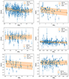 |
Fig. A.1. Individual [Fe/H] measurements and their errors as a function of SMA radius in units of the 2D half-light radius for the dwarf galaxies. The solid orange line and blue shaded area represent the result of the Gaussian process regression analysis (using a Gaussian kernel) and the associated 1-σ confidence interval. The legend box of each panel reports the name of the corresponding dwarf galaxy. |
Appendix B: Consistency checks
B.1. Average metallicity properties
We verified that the global metallicity values calculated for our sample of galaxies (i.e. their weighted average [Fe/H]) agree well with those expected from the stellar luminosity-metallicity relation of Kirby et al. (2013b).
The top left panel of Fig. B.1 shows that the stellar luminosity-metallicity relation obtained by performing a linear fit to our determinations of the global [Fe/H] agrees well with that by Kirby et al. (2013b, their Eq. 3), with the slope and intercept being within ∼ 2-σ from each other. Considering the root-mean-square of the best-fitting line, we found a higher value than was reported by Kirby et al. (0.19 dex versus 0.16 dex), probably due to the different methods used to derive [Fe/H] in our sample. Nevertheless, the two relations show considerable overlap between the scatter regions, demonstrating the absence of a large systematic offset in our sample.
When the linear fit is performed only for galaxies whose [Fe/H] was derived with the CaT calibration method (top right panel), the derived parameters show even better agreement with the Kirby et al. relation (i.e. at ∼ 1-σ level), despite a larger scatter (rms = 0.22 dex) than for the full sample. The absence of significant deviations between the global [Fe/H] of our galaxies and those obtained from the Kirby et al. relation at their luminosity is further evidenced when we take the difference (bottom left panel). We recover a median value of only −0.02 dex for the full sample. Considering the CaT-based measurements, we also recover a low value of 0.02 dex. Therefore, eventual variations in the [Ca/Fe] ratio, inherent to the datasets relying on the CaT-method, do not have a significant impact on the recovery of the average metallicity properties.
We further investigated whether using different ways of quantifying the global metallicity of the galaxies (bottom right panel; see values in Table A.2) may cause significant changes in the stellar luminosity-metallicity relation: we find that using either the median, the weighted average, or the mode of the [Fe/H] distribution function results in very similar relations, at least for the sample of galaxies we considered, but the mode introduces a larger scatter, as is clearly shown in the figure.
 |
Fig. B.1. Comparison of the average metallicity properties of our sample of dwarf galaxies. Top left: Stellar luminosity-metallicity diagram; MW (M31) satellites marked with blue circles (orange squares), while isolated systems are shown as red triangles; the linear relation recovered for our sample is indicated by a dotted line and a rms band in light grey, while a dashed line and rms band in dark grey indicate the Kirby et al. (2013b) relation. Top right: Same as the left panel, but with symbols indicating systems whose ⟨[Fe/H]⟩ have been obtained with the CaT calibration method (orange squares) or using a spectral fitting technique (blue circles); the linear relation recovered for the sub-sample using the CaT method is indicated by a dotted line and a rms band in light grey. Bottom left: Difference between the weighted-average ⟨[Fe/H]⟩ of our galaxies and those obtained from the Kirby et al. (2013b) relation at their luminosity; symbols as in the top right panel. Error bars were obtained adding the ⟨[Fe/H]⟩ errors and the rms = 0.16 dex of the Kirby et al. relation in quadrature. The dashed line is the median offset of 0.02 dex for the sub-sample using the CaT-method. Bottom right: Difference between the weighted average and the median (mode) of [Fe/H] distributions marked with blue squares (orange triangles) as a function of luminosity. The dashed (dotted) lines indicate the rms scatter. |
B.2. Using a different [Fe/H]-CaT equivalent width calibration for Carina and the SMC
We recalculated the individual [Fe/H] measurements for Carina and the SMC, applying the Starkenburg et al. (2010) and Carrera et al. (2013) calibrations, respectively, and compared them with their previous estimates (see Table 1) derived using the Carretta & Gratton (1997) scale. This scale is not optimal at low metallicities.
For Carina (Fig. B.2, left panel), the [Fe/H] distribution is slightly more metal poor than the original by ∼ 0.05 dex, but the calculated gradient remained basically unchanged within the errors. On the other hand, for the SMC (Fig. B.2, right panel), the overall [Fe/H] distribution is more metal poor by ∼ 0.1 dex and the gradient is slightly steeper (−0.130 ± 0.007 dex  , versus −0.101 ± 0.006 dex
  , i.e. different at a 3-σ level). However, we caution that in this case, we needed to use absolute Ks-band magnitudes for the calibration, while apparent magnitudes were provided in the original source (i.e. Dobbie et al. 2014), so differential reddening may be an additional issue here considering its significance in the SMC. Nevertheless, the change in the gradient value for the SMC is small (about 0.05 dex
  ) and does not change the conclusions we have reached in the main text.
B.3. Alternative methods for calculating the gradient
We finally report in Fig. B.3 the results from the comparison between the calculated metallicity gradients ∇[Fe/H](R/Re) used in our analysis and those obtained with an alternative method, namely by calculating the gradient as the difference between the initial value of the GPR curves and that at 2 × Re (in the left panel, while the right panel assumes circular radii; see details in Sect. 5.1 and values in Table A.2). We observe a general good agreement, with 21 (22 for the circular case) out of 30 measurements in agreement within 1-σ, while 29 out of 30 within 2-σ.
 |
Fig. B.2. Comparison of the individual [Fe/H] measurements as a function of SMA radius for Carina (left) and the SMC (right) between the original values (from Koch et al. 2006 and Dobbie et al. 2014, respectively, in black) calculated using the Carretta & Gratton (1997, CG97) scale, and those applying the Starkenburg et al. (2010, S10) and Carrera et al. (2013, C13) calibrations, respectively (in gray). The blue (orange) solid line and shaded area represent the result of the GPR analysis and the associated 1-σ confidence interval to the original (recalibrated) samples. |
 |
Fig. B.3. Difference between the assumed metallicity gradients (on the x-axis) and those calculated between the centre and 2 × Re of the GPR curves, assuming either elliptical (left) or circular radii (right; see Sect. 5.1). Systems for which a difference > 1-σ is recovered are highlighted. |
Appendix C: Orbital parameters
 |
Fig. C.1. Distribution of metallicity gradients as a function of the orbital parameters obtained for the MW satellites, assuming a light potential for the MW (see Battaglia et al. 2022, for further details). On the x-axes we show the eccentricities (top panels), the pericentric distances (middle panels), and the time since the last pericentric passage (bottom panels) of the considered sample. On the y-axes, we plot the metallicity gradients in units of the 2D SMA half-light radius (left panels) and in units of the physical radius (right panels). |
 |
Fig. C.2. As in Fig. C.1, but with the orbital parameters derived assuming a heavy potential for the MW (see Battaglia et al. 2022, for further details). |
We searched for possible correlations between the calculated [Fe/H] gradients and the orbital properties of the MW satellites considered in this work. We inspected the following parameters, made publicly available by Battaglia et al. (2022) and derived using Gaia-eDR3 proper motions (Gaia Collaboration 2021): eccentricity, pericentric distance, orbital period, and time since the last pericentric passage. The inspected parameters were obtained assuming two potentials, treating the MW as isolated: a light potential, with a total mass of M(< Rvir)=8.8 × 10¹¹ M⊙, and a heavy potential, with a total mass of M(< Rvir)=1.6 × 10¹² M⊙. We refer to Battaglia et al. (2022) for further details on the MW potentials and the orbital integration.
As reported in the main text and as shown in Figs. C.1 and C.2, the available sample is too small to reach definitive conclusions on any possible correlation between the metallicity gradients and the orbital parameters. For example, a correlation between ∇[Fe/H](R/Re) and the pericentric distance for both MW potentials is observed. Calculating the Spearman correlation coefficient ρ, we find indeed a high value of ∼ −0.7 in both cases, which is indicative of a strong anti-correlation. While this result may be related to the potential role played by tidal interactions in shaping the radial metallicity profile of satellite galaxies, it is also true that this correlation is mainly driven by the two outermost points, Phoenix and NGC 6822, which also show signs of a past merger event, as we have seen in the main text. Moreover, the orbital parameters of Phoenix are not particularly reliable due to its uncertain 3D velocity (Battaglia et al. 2022). When these dwarfs are removed, ρ noticeably reduces to a value of ∼ −0.4 for both MW-potentials. Therefore, it remains difficult to understand the role of tidal interactions in influencing metallicity gradients.
All Tables
References to the parameters adopted for the systems that are not included in the Battaglia et al. (2022) compilation.
Metallicity averages and radial gradients calculated using circular radii for the systems.
All Figures
|
Fig. 1. Radial metallicity profiles and metallicity gradients calculated for our sample of dwarf galaxies. Top: smoothed [Fe/H] profiles as a function of SMA radius as obtained from the GPR fitting method in units of the 2D half-light radius (left) and as a function of physical radius (right). The radial metallicity profiles have been normalised to their value at R = 0. Dwarf galaxy names are as in Table 1. Bottom: distributions of the calculated metallicity gradients in the same units as in the top panels; bin widths were obtained following the Freedman-Diaconis normal reference rule. |
| In the text | |
|
Fig. 2. Distribution of metallicity gradients as a function of distance from the nearest large LG spiral. Top: satellites of the Milky Way, M31, and the isolated systems are marked as blue circles, orange squares, and red triangles, respectively. Dwarf galaxies that might have experienced a past merger event are marked with an open circle. Bottom: same as above, but with data colour-coded according to their HI content; circles mark a full detection, and squares mark the 5-σ upper limit (data from Putman et al. 2021, and references therein). On the y-axes, the left panels show the metallicity gradients in units of the 2D SMA half-light radius, and in the right panels, they are in units of the physical radius. |
| In the text | |
|
Fig. 3. Distribution of metallicity gradients as a function of the galaxy luminosity in V band with the respective uncertainties. The dashed blue lines represent the linear LSQ fit to the data and the blue shaded areas show the 95% confidence interval. In the legend boxes we report the slope value from the LSQ fits. On the y-axes, the left panel shows the metallicity gradients in units of the 2D SMA half-light radius, while on the right panel, they are in units of the physical radius. Dwarf galaxies that may have experienced a past merger event are marked with an open circle. |
| In the text | |
|
Fig. 4. Distribution of metallicity gradients as a function of the t50 (top panels) and t90 (bottom panels) for our sample of dwarf galaxies. The dashed blue lines represent the LSQ fit to the data and the blue shaded areas show the associated 95% confidence interval. On the y-axes, we plot the metallicity gradients in units of the 2D SMA half-light radius (left panels) and in units of the physical radius (right panels). In the legend boxes we report the slope value from the LSQ fits. Dwarf galaxies that may have experienced a past merger event are marked with an open circle. |
| In the text | |
|
Fig. 5. Luminosity vs. t90 for our sample of dwarf galaxies. Systems that shows significant stellar rotation are marked with triangles, all the others are shown with circles; merger candidates are highlighted with bold text, and the colour-coding and marker sizes are according to the value of their metallicity gradients ∇[Fe/H](R/Re). Dashed red lines identify the sub-regions considered in Sect. 4.4. |
| In the text | |
|
Fig. 6. Comparison with Mercado et al. (2021). Left: metallicity gradients as a function of t50 obtained by Mercado et al. (2021) for a sample of LG dwarf galaxies marked by orange squares with error bars, compared with our determinations for the same sample obtained following the Mercado et al. (2021) criteria (i.e. assuming circular radii and with gradients calculated within 2 × Re, circ) marked by blue circles with error bars. The dashed orange and blue lines are the linear LSQ fits to the described samples, respectively, while the dotted black line (in both panels) is the linear relation found by Mercado et al. (2021) for their set of simulated systems. Right: metallicity gradients obtained again following the Mercado et al. (2021) criteria, but for the full sample of galaxies analysed in this work as a function of their t50 adopted from Weisz et al. (2014), Bettinelli et al. (2018) and Albers et al. (2019); the dashed blue line and shaded area are the linear LSQ fit and the associated 95% confidence interval of the sample, respectively. As reference, red circles mark the sub-sample considered by Mercado et al. (2021). The dashed red line is the linear fit to it. |
| In the text | |
|
Fig. 7. Distribution of the metallicity gradients calculated for the simulated systems presented in Revaz & Jablonka (2018), on the left panel as a function of their stellar mass and color-coded according to their t90, while inverting these two variables in the right panel. Numbers identify the individual halos mentioned in the main text, while the gradient values for the Local Group dwarf galaxies presented in this work are shown as grey circles with their associated error bars. We have assumed in this case a stellar mass-to-light ratio of one. |
| In the text | |
|
Fig. 8. Kernel density estimation of the metallicity gradient distribution for the LG sample (with and without merger candidates as solid and dashed blue lines, respectively), compared with the simulated sets of Revaz & Jablonka (2018, red line) and the DCJL plus MARVEL ones (orange line) analysed in Sects. 5.2 and 5.3, respectively. We assumed in all cases a Gaussian kernel with a bandwidth of 0.04 dex |
| In the text | |
|
Fig. 9. Distribution of the metallicity gradients calculated for the simulated systems of both the DCJL and MARVEL sets as a function of their stellar mass colour-coded according to their t90 (top left) and t50 (top right), and as a function of t90 (bottom left) and t50 (bottom right) in both cases colour-coded according to their stellar mass. We also show the gradient values for the LG dwarf galaxies presented in this work, shown as grey circles with their associated error bars. We have assumed a stellar mass-to-light ratio of one in this case. |
| In the text | |
|
Fig. A.1. Individual [Fe/H] measurements and their errors as a function of SMA radius in units of the 2D half-light radius for the dwarf galaxies. The solid orange line and blue shaded area represent the result of the Gaussian process regression analysis (using a Gaussian kernel) and the associated 1-σ confidence interval. The legend box of each panel reports the name of the corresponding dwarf galaxy. |
| In the text | |
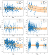 |
Fig. A.2. Same as in Fig. A.1. |
| In the text | |
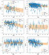 |
Fig. A.3. Same as in Fig. A.1. |
| In the text | |
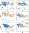 |
Fig. A.4. Same as in Fig. A.1. |
| In the text | |
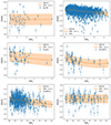 |
Fig. A.5. Same as in Fig. A.1. |
| In the text | |
|
Fig. B.1. Comparison of the average metallicity properties of our sample of dwarf galaxies. Top left: Stellar luminosity-metallicity diagram; MW (M31) satellites marked with blue circles (orange squares), while isolated systems are shown as red triangles; the linear relation recovered for our sample is indicated by a dotted line and a rms band in light grey, while a dashed line and rms band in dark grey indicate the Kirby et al. (2013b) relation. Top right: Same as the left panel, but with symbols indicating systems whose ⟨[Fe/H]⟩ have been obtained with the CaT calibration method (orange squares) or using a spectral fitting technique (blue circles); the linear relation recovered for the sub-sample using the CaT method is indicated by a dotted line and a rms band in light grey. Bottom left: Difference between the weighted-average ⟨[Fe/H]⟩ of our galaxies and those obtained from the Kirby et al. (2013b) relation at their luminosity; symbols as in the top right panel. Error bars were obtained adding the ⟨[Fe/H]⟩ errors and the rms = 0.16 dex of the Kirby et al. relation in quadrature. The dashed line is the median offset of 0.02 dex for the sub-sample using the CaT-method. Bottom right: Difference between the weighted average and the median (mode) of [Fe/H] distributions marked with blue squares (orange triangles) as a function of luminosity. The dashed (dotted) lines indicate the rms scatter. |
| In the text | |
|
Fig. B.2. Comparison of the individual [Fe/H] measurements as a function of SMA radius for Carina (left) and the SMC (right) between the original values (from Koch et al. 2006 and Dobbie et al. 2014, respectively, in black) calculated using the Carretta & Gratton (1997, CG97) scale, and those applying the Starkenburg et al. (2010, S10) and Carrera et al. (2013, C13) calibrations, respectively (in gray). The blue (orange) solid line and shaded area represent the result of the GPR analysis and the associated 1-σ confidence interval to the original (recalibrated) samples. |
| In the text | |
|
Fig. B.3. Difference between the assumed metallicity gradients (on the x-axis) and those calculated between the centre and 2 × Re of the GPR curves, assuming either elliptical (left) or circular radii (right; see Sect. 5.1). Systems for which a difference > 1-σ is recovered are highlighted. |
| In the text | |
|
Fig. C.1. Distribution of metallicity gradients as a function of the orbital parameters obtained for the MW satellites, assuming a light potential for the MW (see Battaglia et al. 2022, for further details). On the x-axes we show the eccentricities (top panels), the pericentric distances (middle panels), and the time since the last pericentric passage (bottom panels) of the considered sample. On the y-axes, we plot the metallicity gradients in units of the 2D SMA half-light radius (left panels) and in units of the physical radius (right panels). |
| In the text | |
|
Fig. C.2. As in Fig. C.1, but with the orbital parameters derived assuming a heavy potential for the MW (see Battaglia et al. 2022, for further details). |
| In the text | |
Current usage metrics show cumulative count of Article Views (full-text article views including HTML views, PDF and ePub downloads, according to the available data) and Abstracts Views on Vision4Press platform.
Data correspond to usage on the plateform after 2015. The current usage metrics is available 48-96 hours after online publication and is updated daily on week days.
Initial download of the metrics may take a while.