| Issue |
A&A
Volume 665, September 2022
|
|
|---|---|---|
| Article Number | A153 | |
| Number of page(s) | 18 | |
| Section | Interstellar and circumstellar matter | |
| DOI | https://doi.org/10.1051/0004-6361/202141511 | |
| Published online | 23 September 2022 | |
The mid-infrared aliphatic bands associated with complex hydrocarbons
1
Department of Physics and Astronomy, Aarhus University,
Ny Munkegade 120,
8000
Aarhus C, Denmark
e-mail: This email address is being protected from spambots. You need JavaScript enabled to view it.
2
School of Engineering and Natural Sciences, University of Iceland,
Dunhagi 3,
107
Reykjavik, Iceland
3
Department of Physics and Astronomy, University of Western Ontario,
London, ON
N6A 3K7, Canada
4
NASA Ames Research Center,
MS 245-6,
Moffett Field, CA
94035-1000, USA
5
Institute of Earth and Space Exploration, University of Western Ontario,
London, ON
N6A 3K7, Canada
6
SETI Institute,
189 Bernardo Avenue, Suite 100,
Mountain View, CA
94043, USA
7
Space Telescope Science Institute,
3700 San Martin Dr.,
Baltimore, MD
21218, USA
8
Department of Physics and Astronomy, University of North Carolina at Chapel Hill,
Chapel Hill, NC
27599-3255, USA
Received:
10
June
2021
Accepted:
11
June
2022
Abstract
Context. The mid-infrared emission features commonly attributed to polycyclic aromatic hydrocarbons (PAHs) vary in profile and peak position. These profile variations form the basis of their classification: Classes A, B, C reflect profiles with increasing central wavelength while Class D has similar central wavelength as Class B but a similar broad shape as Class C. A well-known empirical relationship exists between the central wavelength of these emission features in circumstellar environments and the effective temperature of their central stars. One posited explanation is that the presence of aliphatic hydrocarbons contributes to the variations in the shapes and positions of the features.
Aims. We aim to test this hypothesis by characterising the aliphatic emission bands at 6.9 and 7.25 µm and identifying relationships between these aliphatic bands and the aromatic features.
Methods. We have examined 5–12 µm spectra of 63 astronomical sources exhibiting hydrocarbon emission which have been observed by ISO/SWS, Spitzer/IRS, and SOFIA/FORCAST. We measured the intensities and central wavelengths of the relevant features and classified the objects based on their 7–9 µm emission complex. We examined correlations between the intensities and central wavelengths of the features, both aliphatic and aromatic, and investigated the behaviour of the aliphatic features based on the object type and hydrocarbon emission class.
Results. The presence of the 6.9 and 7.25 µm aliphatic bands depends on (aromatic) profile class, with aliphatic features detected in all Class D sources, 26% of the Class B sources, and no Class C sources. The peak position of the aliphatic features varies, with more variability seen in Class B sources than Class D sources, mimicking the degree of variability of the aromatic features in these classes. Variations are observed within Class D 6–9 µm profiles, but are significantly smaller than those in Class B. While a linear combination of Classes B and C emission can reproduce the Class D emission features at 6.2 and 7.7–8.6 µm, it cannot reproduce the aliphatic bands or the 11–14 µm hydrocarbon features. A correlation is found between the intensities of the two aliphatic bands at 6.9 and 7.25 µm, and between these aliphatic features and the 11.2 µm feature, indicating that conditions required for a population of neutral hydrocarbon particles are favourable for the presence of aliphatic material. A comparison with experimental data suggests a different assignment for the aliphatic 6.9 µm band in Class D and (some) Class B environments. Finally, we discuss evolutionary scenarios between the different classes.
Key words: astrochemistry / molecular processes / infrared: ISM / evolution / ISM: general / ISM: molecules
© P. A. Jensen et al. 2022
 Open Access article, published by EDP Sciences, under the terms of the Creative Commons Attribution License (https://creativecommons.org/licenses/by/4.0), which permits unrestricted use, distribution, and reproduction in any medium, provided the original work is properly cited.
This article is published in open access under the Subscribe-to-Open model. This email address is being protected from spambots. You need JavaScript enabled to view it. to support open access publication.
1 Introduction
Prominent infrared emission features at 3.3, 3.4, 6.2,7.7, 8.6, and 11.2 µm, among others, are observed ubiquitously throughout interstellar space and in many evolved stellar objects. Generally, the carrier of these features can be described as complex hydrocarbons (e.g. Volk et al. 2020). In most environments where these emission features are observed, polycyclic aromatic hydrocarbons (PAHs) dominate the hydrocarbon mixture (e.g. Leger & Puget 1984; Allamandola et al. 1985, 1989a,b; Peeters et al. 2002; Tielens 2008), but the specific identification of PAHs remains controversial. Several other carriers have been proposed, usually with a mix of aromatic and aliphatic hydrocarbons, including hydrogenated amorphous carbon (HAC; e.g. Duley & Williams 1988; Jones et al. 1990) as well as mixed aromatic and aliphatic organic molecules (MAONs; e.g. Kwok & Zhang 2013). The formation process of the proposed carriers is still under debate (e.g. Martínez et al. 2020; Santoro et al. 2020; Kaiser & Hansen 2021).
The spectral profiles and peak positions of the complex hydrocarbon features vary both between objects, and spatially within extended objects. Spectra from the Infrared Space Observatory (ISO; Kessler et al. 1996) led to the classification of hydrocarbon emission in three Classes, A, B, and C, based on their profiles in the 6–9 and 11–14 µm regions (Peeters et al. 2002; van Diedenhoven et al. 2004). Spectra from the Spitzer Space Telescope (Werner et al. 2004) led to a fourth Class, D (Matsuura et al. 2014). Class A spectra generally arise from interstellar objects, for example Hii regions and reflection nebulae, along with a small number of evolved stellar objects. Class B spectra predominantly come from carbon-rich planetary nebulae and the disks around young stellar objects (YSOs). Class C emission arises from a variety of objects, including Herbig AeBe stars, T Tauri stars, carbon-rich objects which have evolved past the asymptotic giant branch (AGB; i.e. post-AGB objects), and carbon-rich red giants. Class D spectra are observed solely in carbon-rich post-AGB objects.
The different classes of hydrocarbon emission profiles reflect variations in the emitting hydrocarbon material from object to object, either structural, chemical, or both. Theoretical studies suggest that the shift between Classes A and B could arise from changes in the size distribution, with smaller hydrocarbon particles responsible for Class A (Bauschlicher et al. 2008, 2009; Cami 2011; Shannon & Boersma 2019). Another hypothesis to explain the differences between Classes B and C is the varying ratio of aliphatic versus aromatic hydrocarbons (e.g. Sloan et al. 2005, 2007; Boersma et al. 2008; Keller et al. 2008; Pino et al. 2008; Acke et al. 2010; Carpentier et al. 2012; Jones et al. 2013; Dartois et al. 2020). In particular, the broadening of the 7.7 µm feature and the shift of this feature and others to longer wavelengths may result from an increasing abundance of aliphatic carbonaceous material. UV processing of complex hydrocarbons will preferentially destroy aliphatic bonds relative to aromatically bonded material. In this case, the degree of aromaticity is linked to the degree of UV photo-processing and thus hydrocarbon emission class. As the material transitions from the environments of evolved stars into the interstellar medium, an increased degree of UV processing then explains an increased degree of aromaticity.
Aliphatically bonded hydrocarbons produce a well-known emission feature at 3.4 µm that accompanies the usually stronger 1–0 C–H stretching mode from aromatic hydrocarbons at 3.29 µm. Geballe et al. (1994) settled the debate over whether the 3.4 µm feature arises from aliphatics or a 2–1 C–H aromatic stretch. They observed the 2–0 transition at 1.68 µm in a planetary nebula and showed that the 3.4 µm feature was much too strong and not at the right wavelength to arise from the 2–1 transition. The presence of the 3.4 µm feature in most Class A and Class B spectra indicates that the observed hydrocarbon mixture is rarely completely aromatic. The open question is whether the aliphatic C–H stretching mode arises from sidegroups attached to the PAH skeleton (e.g. Barker et al. 1987; Geballe et al. 1989; Joblin et al. 1996) or from bonding of H atoms directly to PAHs, which is commonly referred to as superhydrogenated PAHs or HnPAHs (e.g. Bernstein et al. 1996; Sandford et al. 2013), or from the aliphatic component in hydrocarbon solids (which naturally mix aliphatic, aromatic, and olefinic components; e.g. Robertson 1986).
Aliphatically bonded hydrocarbons also produce bands at 6.9 and 7.25 µm due to scissoring motions in methylene (CH2) and methyl (CH3) groups, respectively. Buss et al. (1990) detected the 6.9 µm band in emission in the spectra of warm supergiants, and Tielens et al. (1996) detected it in absorption toward the Galactic center. The launch of ISO led to a flurry of detections of both the 6.9 and 7.25 µm bands in a variety of sources, for example, towards Sgr A* and other sightlines towards the Galactic centre (e.g. Chiar et al. 2000), Herbig Ae/Be stars and post-AGB stars (e.g. Bouwman et al. 2001), and in active galactic nuclei (e.g. Spoon et al. 2001, 2002).
The Spitzer Space Telescope detected the 6.9 and 7.25 µm bands in many more sources (e.g. Sloan et al. 2005, 2007, 2014; Acke et al. 2010; Volk et al. 2011; Matsuura et al. 2014). In evolved stars, the 6.9 µm band is typically stronger than the 7.25 µm band. Matsuura et al. (2014) noted that the 6.9 µm band appears in all Class D sources. Sloan et al. (2014) found that all spectra with the unidentified emission feature at 21 µm also show the 6.9 µm band, and over half also showed the 7.25 µm band. Weak 6.9 and 7.25 µm aliphatic emission could also be identified in a few Class B sources and in one Class A source.
Despite the progress that has been made, a systematic observational analysis of the strengths and positions of the aliphatic bands at 6.9 and 7.25 µm is lacking. This paper seeks to correct that omission with the objective of observationally characterising the aliphatic bands to further our understanding of the nature of the aliphatic carbonaceous material responsible for the bands. We discuss our sources and selection criteria in Sect. 2. Section 3 describes our methodology and Sect. 4 presents the results. We discuss the astrophysical implications in Sect. 5. Finally, Sect. 6 summarises this work and its primary conclusions.
2 Sample
We have compiled mid-infrared spectra of 62 Galactic and Magellanic Cloud sources collected from the literature (Peeters et al. 2002; Sloan et al. 2007; Keller et al. 2008; Bernard-Salas et al. 2009; Cerrigone et al. 2009, 2011; Volk et al. 2011; Matsuura et al. 2014; Sloan et al. 2014) and one previously unpublished spectrum acquired with the FORCAST instrument (Herter et al. 2012) on the Stratospheric Observatory for Infrared Astronomy (SOFIA, Young et al. 2012; Temi et al. 2014). The sources were selected based on the absence of silicate emission at 9.7 µm and their PAH emission characteristics as seen in published spectra obtained with the Short Wavelength Spectrometer (SWS) on board ISO (De Graauw et al. 1996) and the Infrared Spectrograph (IRS) on board Spitzer (Houck et al. 2004). Specifically, we selected (i) all sources known to exhibit aliphatic emission at 6.9 and/or 7.25 and (ii) sources classified as B, C, or D according to the profile of the hydrocarbon emission at 7–9 µm (Peeters et al. 2002; van Diedenhoven et al. 2004; Matsuura et al. 2014) since these are the sources expected to show the strongest evidence of aliphatic emission (Sloan et al. 2007, 2014), but explicitly excluding any sources exhibiting silicate emission (as reported in the cited papers).
Five sources exhibiting Class A or AB band profiles (Peeters et al. 2002; van Diedenhoven et al. 2004) were also included in the sample as their profiles had previously either been mis-classified or their spectra showed some evidence of aliphatic emission1. As we detected aliphatic emission near 6.9 µm in one of these five sources exhibiting Class A or AB spectra, we inspected the remaining Class A and AB sources from Sloan et al. (2014), which are all planetary nebulae (PNe). No evidence of aliphatic emission was found in these spectra. We kept the five sources originally included in the sample, but no more Class A or AB sources were added. Of the 62 sources from the literature, twelve were observed with ISO/SWS, and the remainder with Spitzer/IRS.
We obtained a spectrum of the carbon-rich post-AGB star IRAS 05341+0852 with FORCAST on SOFIA (PI: Peeters, ID 03_0032). The source was chosen because it exhibits an unusually strong aliphatic feature at 3.4 µm (Goto et al. 2007). The observations were carried out using the FORCAST grisms FOR_G063 and FOR_G111 and the 2.4″ wide slit. These grisms cover 4.9–8.0 µm at a resolving power of 180, and 8.4–13.7 µm at a resolving power of 3002.
We determined the object types of the 63 sources in the sample using SIMBAD (Wenger et al. 2000), the SAGE-Spec (Surveying the Agents of Galaxy Evolution: Spectroscopy) Spitzer legacy programme (Woods et al. 2011), and Sloan et al. (2014). Our sample primarily consists of post-AGB objects (35), PNe (18), and Herbig AeBe stars (6). The sample also contains a variable star and an emission line star. A further two sources exhibit a mixture of PN and post-AGB characteristics. Given our sample selection, we are probing many different circumstellar environments. Table 1 presents the full list of sources and their properties.
The sample.
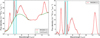 |
Fig. 1 Spectrum of IRAS 06111-7023. Left: a spline continuum is drawn to isolate the emission features. The vertical blue shading denotes regions in which aliphatic emission is often present (near 6.9 and 7.25 µm). Right: the same spectrum after subtracting the spline continuum. |
3 Methods
3.1 Decomposition
We fitted a continuum to each spectrum, utilising a spline function anchored on points adjacent to the complex hydrocarbon features (Fig. 1). This method is common in the literature (e.g Hony et al. 2001; Peeters et al. 2002; Sloan et al. 2005, Sloan et al. 2007). We avoided using an anchor point at ~8.2 µm between the features at 7.7 and 8.6 µm, similar to the method used by Sloan et al. (2014), Shannon et al. (2015), Stock et al. (2016), and Peeters et al. (2017).
After subtracting the spline continuum, we measured the flux of the 6.2 and 11.2 µm features by direct integration. Contributions from the 6.0 and 11.0 µm features were excluded by setting the lower integration boundaries at 6.1 and 11.1 µm respectively. The 6.5–9 µm region was fitted with six Gaussians in order to extract the intensity and central wavelength of the aliphatic bands at 6.9 and 7.25 µm and of the 7.7 µm complex. Figure 2 illustrates the fitting method, which is shown for all sources with aliphatic emission in Appendix B. Specifically, the 6.9 µm aliphatic band can be fitted with a single Gaussian function. However, the 7.25 µm feature is generally blended with the 7.7 µm complex. Consequently, this complex requires five Gaussians, including one for the 7.25 µm feature, akin to the methods of Peeters et al. (2017) and Stock & Peeters (2017). The central wavelength and full-width at half-maximum (FWHM) of each Gaussian function is allowed to vary by up to 0.1 µm to ensure the best fit to the hydrocarbon emission. This step is necessary because the 7.7–8.6 µm complex shifts as a whole, particularly for Class B objects (Peeters et al. 2002). One of the four Gaussian functions fits the 8.6 µm feature; the other three are centred near 7.5, 7.7, and 8.2 µm. We determined the 7.7 µm flux by summing the integrated flux from the Gaussians centred at 7.5, 7.7 and 8.2 µm. The Gaussian at 8.2 µm is incorporated as it sometimes becomes part of the “7.7” µm complex for red-shifted B, C, and D Class profiles (see Fig. 2). The obtained results fit well to the emission in this region, which enables (1) the de-blending of the 7.25 µm band and the 7.7 µm complex, and (2) a good estimate of the total intensity and central wavelength of the 7.7 µm complex. We do not analyse any of the four Gaussians used to represent the 7.7 µm complex individually in this paper. We impose a 3σ detection limit for each band.
Other methods of decomposing the spectra are possible and have been used in the literature. For example, one can fit Drude profiles (PAHFIT, Smith et al. 2007) or Lorentzian profiles (e.g. Boulanger et al. 1998; Galliano et al. 2008) to the individual components in the spectrum. The choice of specific spectral decomposition method may result in the loss of critical information. In addition, the selected decomposition method affects the (absolute) measured fluxes of the hydrocarbon features. Several studies that have employed and compared multiple decomposition methods when studying ratios of hydrocarbon feature strengths have found that the decomposition method does not affect their resulting trends and conclusions (e.g. Galliano et al. 2008; Smith et al. 2007; Peeters et al. 2012, 2017).
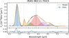 |
Fig. 2 6–10 µm region of IRAS 06111-7023 after subtracting a spline continuum (cf. Fig. 1). The 6.9 µm band is fitted with a single Gaussian, while the complex from 7–9 µm has been fit with five Gaussians, one of which fits the 7.2 µm aliphatic band (see Sect. 3.1 for details). The lower panel shows the residuals after subtracting the fitted Gaussians from the data. |
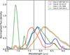 |
Fig. 3 Example spectra for each of the profile classes (in Wm2 µm−1), normalised to the integrated flux of the 7.7 µm feature. The solid vertical lines drawn at 7.7 and 8.2 µm illustrate how the peak wavelength of the 7.7 µm complex changes with profile class. Spectra belonging to Class A peak shortward of 7.7 µm and spectra belonging to Class C peak around 8.2 µm whereas spectra belonging to Classes B or D peak in between. These examples are representative for Classes A and C as those classes only exhibit small variations, but not for Classes B and D. |
3.2 Classification
The central wavelength of the 7.7 µm complex is determined by measuring the bisector of the full Gaussian fit, excluding 7.25 µm where present. Our method differs slightly from that of Sloan et al. (2007, Sloan et al. 2014) in that we include the Gaussian fitted to the 8.6 µm feature to determine the central wavelength of the 7.7 µm complex. Using the central wavelength and shape of the complex, the sources are separated into Classes A, B, C, and D (Peeters et al. 2002; van Diedenhoven et al. 2004; Matsuura et al. 2014). A source is considered to be Class A if the central wavelength of the complex is less than 7.7 µm and if it clearly exhibits a distinct emission feature at 8.6 µm. Class B objects have a redder central wavelength (7.7 µm < λc ⪅ 8.0 µm) and also exhibit a distinct feature at 8.6 µm though it may be significantly more blended or washed out than in Class A objects. Class C objects have very red central wavelengths, λc ~ 8.15–8.2 µm. They generally have a single broad feature from ~7.5 to 9.0 µm rather than showing a separate feature at 8.6 µm. In rare cases, they may exhibit a very weak feature at 8.6 µm. Whether the 8.6 µm feature is absent or blended is unknown (Peeters et al. 2002). The profiles of objects classified as Class D typically have a fairly red central wavelength, though not as red as the C Class spectra. The central wavelength of the 7.7 µm complex of a Class D spectrum generally falls between 7.8 and 7.9 µm. The complex tends to be broadened in a similar way as the Class C spectra, showing a weak to indistinguishable 8.6 µm feature. Figure 3 shows a typical spectrum for each Class taken from our sample. The sample contains three Class A sources, two Class AB3 sources, 43 Class B sources, three Class C sources, and 11 Class D sources.
3.3 The SOFIA spectrum of IRAS 05341+0852
Figure 4 presents the SOFIA spectrum of IRAS 05341+0852. The 6.2 and 11.2 µm emission features are clearly present, as is the 6.9 µm aliphatic band. As the FORCAST grisms do not cover the 8.0–8.4 µm wavelength range, we cannot directly classify its 7.7 µm complex. We utilised a mixture of literature data and indirect measures to help us estimate its profile class, but this analysis was inconclusive and we left this object unclassified in this paper. The Appendix A discusses this analysis more thoroughly.
4 Results
Table 2 presents the fluxes and central wavelengths of the aliphatic bands in sources where they are detected above the 3σ limit. For these sources, we additionally include the fluxes of the 6.2, 7.7 and the 11.2 µm features and the central wavelength of the 7.7 µm feature. In the following sections, we investigate relationships and trends amongst the aromatic features (Sect. 4.1), the aliphatic bands (Sect. 4.2), and relationships between the two sets (Sect. 4.3).
4.1 Aromatics
Band intensities. We recover the well-known strong correlation between the 6.2 and 7.7 µm features, normalising their integrated fluxes to that of the 11.2 µm feature, with a weighted Pearson correlation coefficient of 0.84 (Fig. 5). The observed range of the variations is larger than previously reported in the literature, which includes a sample of Galactic photo-dissociation regions (PDRs) and Hii regions, Magellanic Hii regions, and galaxies of various types (Galliano et al. 2008); Galactic and Magellanic H ii regions and PNe (Bernard-Salas et al. 2009); and the reflection nebulae NGC7023 (Boersma et al. 2014b) and NGC2023 (Peeters et al. 2017). The largest ratios are seen towards seven Classes A or B sources while Classes C and D objects are concentrated towards the lower ratios.
Band profiles
Within the profile classification, Class A and Class C feature profiles only vary slightly between sources, while Class B feature profiles vary much more significantly (Peeters et al. 2002; van Diedenhoven et al. 2004). As our sample contains 11 sources exhibiting Class D emission, we investigated the spectral variations within that class. Figure 6 shows the continuum-subtracted spectra of all Class D sources in this paper. The shape and central wavelength of the 7.7 µm feature profile shows some variation in this group (Figs. 7 and 8). However, while it is larger than the variation observed in Classes A and C, it is significantly less than in Class B. In addition, the central wavelength of the 7.7 µm feature does not vary in unison with the ionisation fraction, as traced by the 6.2/11.2 µm feature ratio. We find a mean central wavelength of 7.81 ± 0.09 µm. Most of the central wavelengths fall between 7.85 and 7.90 µm. However, this average is skewed to the blue due to three sources with central wavelengths below 7.80 µm (IRAS 05413-6934, J01054645-7147053, and NGC 1978). The central wavelengths of the 6.2 and 11.2 µm features of the Class D objects do not vary greatly, although their intensities do vary significantly, though no more than for the other classes (Peeters et al. 2002; van Diedenhoven et al. 2004).
As the profile of the Class D feature is very broad and smooth, we explore whether it can be reproduced by a superposition of a Class B and a Class C profile. As the Class B feature profiles vary significantly (Peeters et al. 2002), the relatively small profile variations in Class D are likely easily accommodated. Figure 9 shows that the average Class D feature profile in the 7-9 µm region closely resembles the superposition of a normalised Classes C with a normalised Class B spectrum. We tested this for 28 Classes B sources in our sample (excluding YSOs) and found that the linear combination accurately recreates the average Class D profile with 11 of these Class B sources. While 10 of the latter 11 Class B sources do exhibit aliphatic emission at 6.9 µm, it is not possible to recreate the strong aliphatic 6.9 µm band seen in most Class D spectra. Furthermore, we found that blue B profiles (i.e., peaking towards the blue end of the observed B Class wavelength range) recreate the average Class D spectrum best, whereas red Class B profiles will tend to create a spectrum with the right shape, but peaking to the red of any Class D profiles in our sample. A linear combination between an A and C profile also yields roughly the shape of a D profile, but it peaks to the blue of most D profiles in our sample. A similar effort found that a linear combination of Classes B and C could not accurately recreate the shape of the Class D profile in the 10–14 µm wavelength range.
In terms of object type, the Classes C and D sources in the sample are all post-AGB objects, which suggests that these spectra are seen primarily in circumstellar environments where significant mass loss and dust formation has recently taken place. The Class A sources in the sample are a mix of post-AGB objects and PNe while the Class B sources contain a mixture of many different object types including Herbig AeBe stars, post-AGB objects, and PNe. All Herbig AeBe stars in our sample exhibit Class B emission.
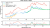 |
Fig. 4 Our SOFIA spectrum of IRAS 05341+0852 (blue) is compared to other spectra from the literature, including another SOFIA spectrum (orange; Materese et al. 2017), a Spitzer/IRS spectrum (AORkey: 4896512, PI: Dale Cruikshank), and an ISO/SWS spectrum (Matsuura et al. 2014). The dashed lines represent the applied continua for the corresponding spectra (in the same colour). The lower panel displays the residual after subtracting a spline continuum. See Sect. 3.3 for details. |
Intensities and central wavelengths of sources with aliphatic emission detected at or above S/N = 3.
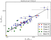 |
Fig. 5 Correlation between the intensity of the 6.2 and the 7.7 µm features, normalised to the intensity of the 11.2 µm feature. We recover the well-known correlation between the features and find a correlation coefficient r = 0.84. |
4.2 Aliphatics
Here we present the results pertaining to the aliphatic bands at 6.9 and 7.25 µm. As discussed in Sect. 5.1, an aromatic component at 6.67 µm and a potential olefinic component at 7.09 µm may contribute, respectively, to the 6.9 and 7.25 µm bands analysed here. Given the spectral resolution of the data used in this paper, we are unable to discern potential contributions of a non-aliphatic nature. Based on prior observations, we anticipate their contributions to be minimal. An emission feature at 6.9 µm is present at or above 3σ in 24 sources, and a feature at 7.25 µm is present at or above 3σ in 14 of those 24 sources. Table 2 lists those sources.
The central wavelength, λc, of the 6.9 µm band varies continuously from 6.80 to 6.95 µm (with two outliers at slightly redder wavelengths, and one at slightly bluer wavelength) with an average of 6.91 ± 0.05 µm. This behaviour is consistent with reported values in the literature (Table 3). However, within the individual profile classes, this picture changes (Fig. 10). For Class B sources, the peak wavelength varies continuously across the observed 6.80–6.95 µm range, but for Class D sources the variation is, while still present, more limited. The feature in the Class A source is close to the average. Since only one Class A source in our sample exhibits aliphatic emission, it is impossible to generalise about the behaviour of the band within this class. Acke et al. (2010) reported a FWHM for the 6.9 µm band of 0.11 ± 0.04 µm whereas we find a generally wider FWHM of 0.16 ± 0.03 µm. As noted by Matsuura et al. (2014) and Sloan et al. (2014), all Class D sources show 6.9 µm emission. Within this class, its strength varies significantly, that is, from 20 to 150% of the 6.2 µm band strength. In a handful of sources (e.g. IRAS F05110, IRAS 06111, J004441, and NGC 1978), the peak flux density of the 6.9 µm aliphatic band is stronger than that of the 6.2 µm aromatic feature. Thus, it is typically much stronger than the 6.9 µm band intensity observed in other profile classes (Sloan et al. 2014).
While most detections of the 6.9 µm features have signal-to-noise ratios (S/N) larger than 10, many of the 7.25 µm band detections have S/Ns of only ~3 or 4, making them significantly weaker than their 6.9 µm counterpart. Furthermore, the 7.25 µm band is blended with the blue wing of the 7–9 µm complex and has to be disentangled before it can be characterised, leading to larger uncertainties in its flux and peak wavelength. The 7.25 µm band is detected in only 58% of the sources with 6.9 µm emission. Figure 11 shows the 7.25 µm band profiles and their average. The position of the band varies more than the 6.9 µm band. The central wavelength varies from 7.17 to 7.31 µm with an average value of 7.26 ± 0.04 µm. Of the 14 detections of the feature, seven are from Class B sources, and seven from Class D sources. The class-dependent average positions of the feature are 7.24 ± 0.04 µm for Class B and 7.28 ± 0.02 µm for Class D. Previously, the central wavelength of this feature has been measured as 7.22 ± 0.02 µm (Acke et al. 2010) and 7.27 ± 0.02 µm (Sloan et al. 2014) (see Table 3). Our results are entirely consistent with the literature, given that the sample of Acke et al. (2010) contains only Class B objects, and Sloan et al. (2014) primarily detected a 7.25 µm band in Class D sources. Acke et al. (2010) reported a FWHM of 0.11 ± 0.03 µm for the 7.25 µm band. We found a FWHM of 0.11 ± 0.03 µm in excellent agreement with previously reported results.
Finally, we examined correlations between the aliphatic emission bands. Figure 12 shows the correlations between the intensities of the two aliphatic bands, normalised to the intensity of the 6.2 µm feature. Given the limited amount of sources (i.e. 14), we find a reasonable correlation (with Pearson correlation coefficient r = 0.86), although we note that this is largely driven by the Class D sources.
4.3 Aliphatics versus aromatics
We investigated possible correlations between the aliphatic bands and aromatic features. We found a very weak correlation between the intensities of the 7.25 aliphatic band and 11.2 µm aromatic feature, normalised to the intensity of the 6.2 µm feature, with a weighted Pearson correlation coefficient of r = 0.60 (Fig. 13). We find a stronger correlation between the intensities of the 6.9 band and the 11.2 µm feature when normalising to the intensity at 6.2 µm, with a weighted Pearson correlation coefficient of r = 0.84 (Fig. 13). However, if we only consider sources exhibiting both a 6.9 and a 7.25 µm band the correlation improves and we find a correlation coefficient of r = 0.92. Hence, the intensity of the 6.9 and 7.25 µm aliphatic bands correlates with the 11.2 µm PAH intensity.
The ratio of the 11.2 µm out-of-plane bending mode to either the 6.2 or 7.7 µm C–C modes in PAHs traces the degree of ionisation of the PAHs (e.g. Allamandola et al. 1985, 1999; Hudgins et al. 1994), with a higher ratio indicating a higher ionization fraction. Thus this correlation suggests that the aliphatic bands tend to be stronger in environments where the PAHs are more neutral.
Figure 14 shows the correlations of the two aliphatic bands with the 7.7 µm complex. A weak correlation (r = 0.61) is found for the 6.9 µm band, while no correlation (r = 0.38) is found for the 7.25 µm band.
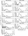 |
Fig. 6 Continuum-subtracted spectra of the Class D sources in our sample. The aliphatic feature at 6.9 µm is found in all 11 sources, and is comparable in strength to the 6.2 µm feature for a number of them. The aliphatic feature at 7.25 µm is unambiguously measured in seven of the sources. |
4.4 Wavelength correlations
No convincing correlations were found between the peak wavelengths of the aliphatic bands, nor between the peak wavelengths of the aliphatic bands and the central wavelength of the 7.7 µm complex (see Sect. 3.2 for definition, Fig. 15). We checked for a potential correlation between the peak wavelength of the aliphatic features and the effective temperature of the star where these data are available, but find no correlation. Whether this is an intrinsic result or a consequence of the small sample size is not yet possible to determine.
Lastly, we checked the correlation between the ratio of aliphatic-to-aromatic intensities and the central wavelength of the 7.7 µm feature. The 7.7 µm feature has previously been shown to correlate with effective temperature for Classes A, B, and C (Sloan et al. 2007; Keller et al. 2008; Acke et al. 2010), and Acke et al. (2010) found a correlation between the aliphatic-to-aromatic intensity ratio and effective temperatures in YSOs. Figure 16 shows our results. We find no overall correlation.
However, the Class B sources as a group do exhibit a correlation. In contrast, the aliphatic-to-aromatic ratio seems to be independent of the central wavelength of the 7.7 µm complex for Class D sources (see Sect. 3.2 for definition).
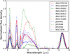 |
Fig. 7 All Class D spectra normalised to the peak flux of the 11.2 µm feature. The shape and strength of the 7.7 µm complex vary significantly, but the peak position of the complex does not. Additionally, the strength of the 6.2 and 7.7 µm features vary together, suggesting that the peak positions of the features do not change with ionisation fraction. |
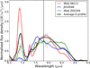 |
Fig. 8 Average Class D profile spectrum (in Wm−2 µm−1), normalised to the flux of the 7.7 µm feature (solid black line). The vertical line marks the average peak wavelength of the 7.7 µm complex for Class D spectra (i.e. 7.8 µm). The three Class D spectra that showed the most deviation from the average are shown in red, blue, and green. Aliphatic bands are present at 6.9 and 7.25 µm. |
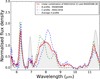 |
Fig. 9 Linear combination (solid red line) of Class B and Class C spectra (dashed green and blue respectively), both of which are normalised to the integrated flux of the 7.7 µm complex. The average Class D profile spectrum, also normalised to the integrated flux of the 7.7 µm complex, is filled in in grey for comparison. |
Centroid averages for the aliphatic emission bands.
5 Discussion
We have systematically investigated the relationship between the aliphatic hydrocarbon bands at 6.9 and 7.25 µm and the aromatic hydrocarbon features in the mid-IR. Here we discuss the implications for their carriers and put it in context of previous observations, theory, and experiments. We note that observations at 3 – 4 µm cover both aromatic and aliphatic emission and, combined with our study, would provide a more complete assessment of the observational characteristics of the aliphatic features. Unfortunately, such observations are unavailable for our sample, restricting the discussion to the mid-IR features.
Our findings can be summarised as follows: Firstly, we confirmed the association between Class D emission and aliphatic emission at 6.9 µm as previously reported by Matsuura et al. (2014) and Sloan et al. (2014). Secondly, we failed to detect aliphatic emission above 3σ in any Class C sources. However, we only considered post-AGB objects and did not investigate YSOs (due to the presence of silicate emission in the latter). Third, we found a correlation between the strengths of the aliphatic hydrocarbon emission bands at 6.9 and 7.25 µm and the aromatic out-of-plane bending mode at 11.2 µm. The 11.2 µm feature is stronger with respect to the aromatic skeletal modes at 6–9 µm when neutral PAHs dominate the PAH population, suggesting a connection between aliphatic emission and a softer radiation field. Additionally we found that a linear combination of Classes B and C can reproduce the Class D emission profile at 7–9 µm, when blue Class B spectra are used. However, this combination does not reproduce Class D emission at 11–14 µm nor does it reproduce the strong aliphatic band at 6.9 µm observed in all Class D sources. And lastly we found that the position of the 6.9 µm aliphatic band is confined to the immediate vicinity of 6.90 µm in Class D sources, but when it appears in Class B sources, its peak position varies between 6.80 and 6.90 µm.
These findings, put in the context of previous work, can shed light on two important questions about interstellar PAHs and carbonaceous material: (1) the origin of the aliphatic bands observed in many hydrocarbon spectra of late-type stellar objects, and (2) what clues the aliphatic emission bands provide about the evolution of the hydrocarbon population with profile class.
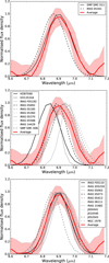 |
Fig. 10 Average 6.9 µm profile based on 24 spectra with a 3σ detection of this band (red). The envelope on the average feature represents a 1σ variation in the profile. The individual 6.9 µm band profiles of SMP SMC Oil (Class A) and IRAS 05341 (Class undetermined) (top), Class B (middle) and Class D (bottom) are shown in grey-scale. For Class B, a representative sample is shown for clarity. The band profiles (in Wm−2 µm−1) were normalised to the fitted peak flux densities of the features. |
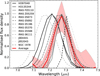 |
Fig. 11 Average 7.2 µm band profile (in Wm−2 µm−1), based on 14 spectra with a 3σ detection of this band, normalised to the fitted peak flux density (in red). The shaded region represents the standard deviation of the average profile. The individual, normalised 7.25 µm band profiles are shown in grey-scale. |
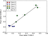 |
Fig. 12 Correlation between the intensities of the 6.9 and 7.2 µm features in sources containing both features, normalised to the intensity of the 6.2 µm band. A 3σ cut was applied to the intensity ratios. The correlation coefficient is 0.86. |
5.1 Assignments for the aliphatic emission features
The emission band from aliphatic hydrocarbons at 6.9 µm arises from a scissoring transition in methylene units (CH2, Wexler 1967). Its position depends on the number of neighbouring methylene units. In aliphatic chains, it appears near 6.8 µm while in larger, primarily aromatic molecules with only a few methylene subunits, it appears at 6.9 µm or even at longer wavelengths (Colthup et al. 1990; Arnoult et al. 2000). The 6.9 µm band behaves similarly in HnPAHs, shifting from ~6.9 µm in PAHs with few additional H atoms to ~6.8 µm in more completely hydrogenated PAHs (Sandford et al. 2013). The band also grows stronger with increasing levels of hydrogenation. In addition to this band, Jones et al. (2013) suggest that an asymmetric sp3 CH3 C–H bending mode at 6.8 µm and an aromatic CC mode at 6.67 µm may contribute to the 6.9 µm feature. The relative contributions of the individual sub-bands vary with the chemical structure of the emitting population of molecules and determine the peak position of this blended feature.
A weaker band at 7.2–7.35 µm arising from methyl groups (Chiar et al. 2000) is generally also present in the laboratory spectra of HnPAHs and PAHs with aliphatic side-groups and side-chains. Specifically, Jones et al. (2013) note that multiple bands can contribute at this wavelength, including aliphatic sub-bands at 7.14 and 7.30 µm arising from methyl groups, and possibly an olefinic band at 7.09 µm. The presence of this band in astronomical spectra thus implies the presence of methyl sidegroups in PAHs, longer chains, or complex hydrocarbons. Thus, we expect PAHs with excess hydrogen atoms or aliphatic sidegroups, or amorphous hydrocarbon material with strong aliphatic components, to exhibit emission at 6.9 and 7.25 µm with the position of the former feature depending on the relative contribution of the aliphatic and aromatic bonds within the hydrocarbon mixture.
The difference in the behaviour of the 6.9 µm band between the Classes B and D spectra suggests differences in the aliphatic hydrocarbons between these two classes. For most Class D sources, the 6.9 µm band is centered close to 6.9 µm, while for Class B sources with aliphatic emission, the peak of the feature spans a range of wavelengths and is significantly blue-shifted for many Class B sources. As Fig. 14 shows, the 6.9 µm band is significantly stronger in the Class D spectra. Combined with the experimental results, this implies that most Class D sources have aliphatic emission due to completely hydrogenated HnPAHs or other hydrocarbon structures with a significant aliphatic component, or larger, primarily aromatic molecules with only a few methylene subunits. In addition, the blue-shifted aliphatic component seen in many Class B sources arises from either minimally hydrogenated HnPAHs or from short sidechains (with few or no neighbouring methylene groups). We note that this change is not correlated with the 7.7 µm band profile (Fig. 15).
The composition of the hydrocarbon material is interesting from an evolutionary standpoint, but it may also be particularly important for H2 formation. Due to their high abundances, PAHs provide a large fraction of the total available surface area for the formation of H2 via surface reactions (Habart et al. 2003, 2004). Laboratory and theoretical studies show that the creation of HnPAHs, and subsequent abstraction of excess hydrogen atoms through Eley-R2ideal type reactions (forming H2 in the process), is a possible formation route under astrophysical conditions (Bauschlicher 1998; Rauls & Hornekær 2008; Thrower et al. 2012, Thrower et al. 2014; Mennella et al. 2011; Skov et al. 2014; Jensen et al. 2019). Photolysis of HAC is another possible route towards the formation of H2 under interstellar conditions (Jones & Habart 2015) that may be relevant in the environments of interest in this paper. In this scheme, a single UV photon will dissociate a CH bond in an aliphatic or olefmic bridge between aromatic clusters in the amorphous grains, freeing up a hydrogen atom to bond with a bound hydrogen atom from a different CH group. Observationally, a correlation between hydrocarbon emission and the H2 formation rate has been observed in PDRs (Habart et al. 2003, 2004). It should however be noted that while a feature at 3.4 µm has been observed in a number of PDRs, aliphatic bands at 6.9 or 7.25 µm have neither been reported nor studied in those sources, nor are there any observational studies that suggest a similar correlation in the late-type stellar objects studied here.
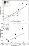 |
Fig. 13 Intensities of the 6.9 (top) and 7.25 (bottom) µm bands compared to the 11.2 µm feature intensities normalised to the intensity of the 6.2 µm feature. Filled markers represent sources where both aliphatic bands have been detected, while unfilled markers represent sources where only the 6.9 µm band has been detected. For the 6.9 µm band, the correlation coefficient is 0.84, and improves to 0.92 when only considering sources where both aliphatic bands are detected. For the 7.25 µm band, a weak correlation with a correlation coefficient of 0.60 is found. |
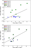 |
Fig. 14 Intensities of the 6.9 (top) and 7.25 µm (bottom) aliphatic bands compared to the 7.7 µm feature intensities normalised to the intensity of the 6.2 µm feature. Filled markers represent sources where both aliphatic features have been detected, while unfilled markers represent sources where only the 6.9 µm feature has been detected. The correlation coefficient is 0.84 and 0.38 for the 6.9 and 7.25 µm bands, respectively. |
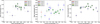 |
Fig. 15 Central wavelengths of the 6.9 versus 7.25 µm bands (left), the 6.9 band versus the 7.7 µm feature (center), and the 7.25 band versus the 7.7 µm feature (right). No convincing correlations are observed. |
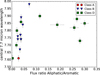 |
Fig. 16 Correlation between the ratio of aliphatic to aromatic intensities and the central wavelength of the 7.7 µm feature. A 3σ cut was applied to the intensity ratios. The correlation coefficient is 0.55 for Class B, but no correlation was found for Class D. |
5.2 Structural and chemical evolution of the emitters
It is generally accepted that the profile classes reflect an evolution in the structural and/or chemical state of the emitting population (Peeters et al. 2002; van Diedenhoven et al. 2004; Sloan et al. 2007; Bauschlicher et al. 2008, 2009; Keller et al. 2008; Pino et al. 2008; Acke et al. 2010; Cami 2011; Carpentier et al. 2012).
Theoretically calculated intrinsic PAH spectra have illustrated that the peak position of the various features in the 6–9 µm range depends on PAH size and to a lesser degree PAH charge and structure (e.g. Bauschlicher et al. 2008, 2009; Ricca et al. 2012; Peeters et al. 2017). Cami (2011) reported excellent fits of the Classes A, B, and C PAH emission using the NASA Ames PAH IR spectral database (Bauschlicher et al. 2010, Bauschlicher et al. 2018; Boersma et al. 2014a) indicating Class C PAH emission is reproduced by the emission of a collection of small PAHs. More recently, Shannon & Boersma (2019) systematically analysed employing this PAH database and concluded that PAH size drives the difference in Classes A and B emission. These authors were unable to reproduce the Classes C and D emission.
Based on the observed dependence of the central wavelength of the aromatic emission features with the effective temperature of the central star, the variation in profile classes have also been attributed to a varying degree of aromaticity (Sloan et al. 2007; Keller et al. 2008; Acke et al. 2010). Laboratory studies of soot and hydrocarbon material of varying aliphatic content provide further evidence for this hypothesis (Pino et al. 2008; Carpentier et al. 2012). As the aliphatic content increases, the strength of the aliphatic bands at 3.4 and 6.9 µm grows, though the latter remains weak. A higher aliphatic content also shifts the 6.2 µm emission feature to the red (by ~0.1 µm) and shifts the 7–9 µm emission complex from a spectral shape and structure most closely resembling Classes A, then B, and then C. These results suggest that the Class C emission arises from hydrocarbons with higher aliphatic-to-aromatic ratios than Class B.
The laboratory results and the observations differ in two significant ways. First, with increasing degree of aromaticity, the overall spectrum changes with emission features dominating at lower aliphatic fractions and the continuum emission dominating at higher fractions. Second, even for a high degree of aliphatic content, the aliphatic bands at 6.9 and 7.25 µm remain weak in the laboratory samples (Carpentier et al. 2012). These differences in part arise from the size of the soot particles. More recent laboratory results (Dartois et al. 2020) may address the aliphatic bands seen in observed Class D spectra. These authors applied a top-down approach to studying astronomical hydrocarbon analogues by mechanical milling various types of microscopic carbon solids (e.g. graphite, carbon nanotubes, multi-layer graphene, and C60) in a hydrogen atmosphere, to mimic the very localised chemical reactions with solids happening in interstellar space. Increased milling times led to a stronger aliphatic emission component in the spectra. These samples reproduce the strong feature observed at 6.9 µm observed in Class D astronomical spectra and convincingly recreate Classes C and D emission profiles. Increased milling also led to an increase in curvature and defects in the hydrocarbon material, which influences the shape of the 7–9 µm emission complex. Details in the structure depend on the overall H-content in the sample, and a H-content of 3–7% best fits the astronomical spectra. Dartois et al. (2020) suggest that the carriers of the Classes C and D spectra may represent an intermediate evolutionary level between small carbonaceous dust particles and pure free-floating PAH molecules, with Class D emitters being comprised of free-floating, well-defined (mostly aromatic) PAH molecules.
With these laboratory and theoretical results in mind, we discuss an evolutionary scenario from Class C to Class D, then to Class B, and finally to Class A in the environments surrounding evolved stars. Several results support this scenario: (1) acetylene, a building block in the bottom-up PAH formation route, and benzene are only detected in some Class C sources (Kraemer et al. 2006; Sloan et al. 2007); (2) Class D profiles at 7–9 µm can be reconstructed by a superposition of a (blue) Class B and Class C profile, but not by a Class A and a Class C profile; and (3) Class B and Class D sources show aliphatic emission at 6.9 and/or 7.25 µm. However, a number of arguments can also be made against this scenario: (1) Class C exhibits weak to no emission assigned to CH modes (both aromatic and aliphatic, van Diedenhoven et al. 2004; Kraemer et al. 2006; Sloan et al. 2007) whereas the other classes do. Hence, the origin of the hydrogen present in Class D (and subsequently Classes B and A) is unclear in this scenario; (2) we cannot reproduce the strong 6.9 µm emission feature seen in Class D with a linear combination of any Classes C and B sources; (3) both Classes B and C are readily seen in different types of YSOs, but not Class D which is the intermediate step between Classes B and C in the scenario outlined above.
Another possibility is that Classes C and D represent a fork in the astronomical PAH evolution, i.e., instead of going from C to D to B to A, the evolution goes from C or D to B to A. In this case, local variations in the chemical and physical environment, including different lines of sight, determine whether Classes C or D emission is observed. For example, Class C may require a higher optical depth, consistent with the observed absorption bands from acetylene and other smaller molecules seen in some spectra. Such a difference in optical depth can arise for different inclinations in an axisymmetric morphology, with Class D being observed with more pole-on angles and Class C being observed with more edge-on angles.
The James Webb Space Telescope (JWST) will simultaneously provide full wavelength access relevant to PAH emission (3–20 µm) at medium spectral resolution (required for the characterisation of substructure or blended PAH emission bands), at high spatial resolution (required to disentangle the response of PAHs to the changing physical conditions) and with high sensitivity. This capability will enable a systematic study of the (often weaker) aliphatic emission bands and their relation to the aromatic emission features. It will also allow for the investigation of potential olefinic bands. To fully exploit the data that JWST will produce, additional experimental and theoretical studies are essential. In particular, systematic experimental and/or theoretical studies of PAHs with excess hydrogenation, hetero-atoms, and with and without sidegroups, which more closely resemble those expected to be present in space in size and shape, would make for better comparisons. Furthermore, systematic experimental and/or theoretical studies of the dynamics governing the interaction of PAHs in space with atomic species, radicals, free electrons, and radiation are required to interpret the evolution of the carrier of the aliphatic bands in extended sources.
6 Conclusion
We present a systematic study of the characteristics of the aliphatic carbonaceous emission bands at 6.9 and 7.25 µm and their relation to the aromatic emission features from complex hydrocarbon in late-type stellar objects and YSOs these features are commonly attributed to PAHs. The aim is to study the origins of the aliphatic features as well as their relations to the hydrocarbon profile classes. To this end, we compiled a sample of 63 sources exhibiting complex hydrocarbon emission, most of which belong to profile Classes B, C, or D. We detected aliphatic emission features in 24 sources, all of which exhibit emission at 6.9 µm and 14 of which exhibit emission at 7.25 µm.
Due to its relative recent discovery, we explored the characteristics of the 7.7 µm Class D profile. We find that this profile shows some variability, but it is significantly less than that present in Class B. Moreover, the average 7–9 µm Class D profile closely resembles a linear combination of Classes B and C profiles.
We confirm that the presence of the 6.9 and 7.25 µm aliphatic bands depends on (aromatic) profile class, with aliphatic features detected in all Class D sources, 26% of the Class B sources, and no Class C sources. Only one of the five Class A or AB sources present in our sample has aliphatic bands in its spectrum.
We report variability in terms of peak position for both aliphatic bands. The peak positions of the 6.9 and 7.25 µm bands vary continuously from 6.8 to 6.95 µm and from 7.22 to 7.28 µm respectively. This variation is much more pronounced in Class B sources than in Class D sources. Hence, the degree of variability mimics that which is seen in the aromatic feature profiles for a given profile class. However, no convincing correlations are present between the peak position of these aliphatic bands and that of the 7.7 µm complex.
Considerable variation is also seen in the strength of the aliphatic bands, especially at 6.9 µm. The band is strongest in Class D sources. In some cases within Class D, the 6.9 µm band is stronger than the 6.2 µm feature, indicating that the hydrocarbon material in Class D objects is likely more aliphatic in nature than that in other classes.
We further explored possible correlations between aliphatic and aromatic emission feature intensities. We find strong to moderate correlations between the strengths of the aliphatic 6.9 µm and 7.25 µm bands and the 11.2 µm aromatic feature. This suggests that aliphatic material is more likely to be present where the PAH population is primarily neutral.
The aliphatic material may be in the form of HnPAHs, aliphatic sidegroups on (neutral) PAHs or separate aliphatic molecules present along with a neutral PAH population. Comparison with experimental data suggests that most Class D sources have aliphatic emission due to completely hydrogenated HnPAHs or larger, primarily aromatic molecules with only a few methylene subunits. In contrast, the blue-shifted aliphatic component seen in many Class B sources may arise from either minimally hydrogenated HnPAHs or from short sidechains (with few or no neighbouring methylene groups). We find that this change is not correlated with the 7.7 µm feature profile. Finally, we explore two evolutionary scenarios: an evolutionary sequence from Classes C to D to B to A and evolutionary sequence from Classes C or D to B to A. We conclude that future observations from e.g., JWST, are required to settle this issue.
Acknowledgements
The authors would like to thank Drs. L. Keller, K. Volk, M. Matsuura, and M. Goto for providing data used in this article. We thank the referee, A. Jones, for helping us improve this paper. The authors would also like to acknowledge funding from the Independent Research Fund Denmark under grant no. 4002-00385B, the Augustinus Foundation, the Oticon Foundation, and the Natural Sciences and Engineering Research Council of Canada (NSERC).
Appendix A The SOFIA spectrum of IRAS 05341+0852
Fig. 4 presents our SOFIA spectrum of IRAS 05341+0852, which we acquired using the FORCAST grisms. The 6.2 and 11.2 hydrocarbon emission features are clearly present, as is the 6.9 aliphatic band. As the FORCAST grisms do not cover the 8.0–8.4 range, we cannot directly classify its 7.7 complex. Instead, we examined data from the literature and considered indirect measures to help classify the hydrocarbon spectrum.
Fig. 4 includes spectroscopic observations of IRAS 05341 from the literature. These data include an ISO/SWS spectrum from Matsuura et al. (2014), a Spitzer/IRS high-resolution spectrum (AORkey: 4896512, PI: Dale Cruikshank), and a cross-dispersed SOFIA FORCAST spectrum from Materese et al. (2017). The ISO/SWS spectrum has complete spectral coverage in our region of interest, albeit with a somewhat lower signal-to-noise ratio. The high-resolution, high-sensitivity Spitzer spectrum provides reliable data, but no coverage below 10 µm. The SOFIA spectrum by Materese et al. (2017) has the same limitations as our data, but it allows a direct comparison of the 6.2, 6.9, and 11.2 features and the overall continuum. Due to low signal-to-noise, we smoothed the SWS and SOFIA data for this comparison. To directly compare the hydrocarbon features, we subtracted a spline continuum from the data, as shown in the lower part of Fig. 4. Given the limitations of each data set, the spectra agree fairly well with each other. The 6.2 feature is clearly present, though its width seems particularly inflated in the SWS spectrum. The 11.2 feature is very consistent (in both shape and absolute calibration) between our SOFIA spectrum and the Spitzer spectrum. The 11.2 feature in the SWS spectrum, however, is affected by serious spectral undulations, which is not unusual for this wavelength range (at the end of band 2C in SWS AOT1 spectra).
Considering the 7.7 feature, the SWS spectrum suggests that IRAS 05341 may be a class D source, as first noted by Matsuura et al. (2014). In their spectrum (shown here), the profile starts at roughly 6.6 whereas a typical class D profile (Fig. 9) starts at ~7.15 when taking a continuum anchor point around the 6.9 band as done in this paper. However, even after considerable smoothing, the SWS spectrum has an unusual appearance, and an anchor point near 7.15 would produce extreme curvature in the continuum that we do not expect to be present. Our SOFIA spectrum instead is suggestive of a class C profile, though the limited signal-to-noise of these data as well and the gap in wavelength coverage leave the classification somewhat ambiguous.
We can also use indirect measures to narrow down to the 7.7 class. First, we measured the peak wavelengths of the 6.2 and 11.2 features, which depend on profile class (Peeters et al. 2002; van Diedenhoven et al. 2004). Specifically, both features are red-shifted for class B and C objects compared to class A, and are red-shifted to a higher degree for class C objects. We note that class D objects were not included in these studies and thus this relationship has not been established for class D sources. For the SOFIA spectrum, we find λp(6.2) = 6.27 ± 0.02 µmand λp(11.2) = 11.35 ± 0.02 µm. Both of these peak wavelengths are significantly red-shifted compared to what is expected for these features in a class A spectrum. The wavelength of the 6.2 feature is within the range found for class B profiles, but at the red end and thus close to that of a class C profile. The 11.2 feature is more red-shifted than a typical class B feature (Peeters et al. 2002; Sloan et al. 2007). In addition, in the sample of Sloan et al. (2007), sources with central wavelengths for the 6.2 and 11.2 features similar to those measured for our SOFIA spectrum of IRAS 05341 have central wavelengths between 8.15 and 8.25 for the 7.7 complex. Thus the peak wavelengths point toward a red B or C class profile.
Second, it is well established that the central wavelengths of the 6.2, 7.7, and 11.2 features, and thus the profile classes, correlate well with effective stellar temperature for hydrocarbon in circumstellar environments (Sloan et al. 2007; Keller et al. 2008). Based on a small sample of three sources, Matsuura et al. (2014) found however that class D sources do not follow this relationship. With an effective temperature of 6750 ± 125 K (De Smedt et al. 2016), IRAS 05341 coincides with effective temperatures in the overlap region between class B and C for both the 7.7 and 11.2 features (see Fig. 8 of Keller et al. 2008). Using this relationship, we find an expected central wavelength of ~8.1 and ~11.35 µm for the 7.7 and 11.2 µmfeatures, respectively. In addition, in the sample of Sloan et al. (2007), sources with central wavelengths for the 6.2 and 11.2 features similar to those measured for our SOFIA spectrum of IRAS 05341 exhibit central wavelengths of between 8.15 and 8.25 for the 7.7 complex. The central wavelengths of these features suggest that IRAS 05341 is a class C object.
We conclude that IRAS 05341+0852 likely has a 7.7 µm complex that is most consistent with that of a class C profile. As the indirect measures do not apply to class D sources, we cannot confidently exclude the possibility that it is a class D source. Due to this ambiguity, we leave its profile class as undetermined for this paper.
Appendix B Gaussian decomposition
We provide the full set of fits to sources with aliphatic features in Figs. B.1, B.2 and B.3. The methodology is as described in Section. 3.1.
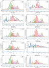 |
Fig. B.1 Complete fits to our sources with aliphatic features. The number at the top of the y axis (e.g. 1e-15) refers to the multiplication factor for the values on the axis. |
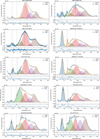 |
Fig. B.2 Complete fits to our sources with aliphatic features. The number at the top of the y axis (e.g. 1e-15) refers to the multiplication factor for the values on the axis. |
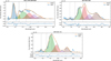 |
Fig. B.3 Complete fits to our sources with aliphatic features. The number at the top of the y axis (e.g. 1e-15) refers to the multiplication factor for the values on the axis. |
References
- Acke, B., Bouwman, J., Juhász, A., et al. 2010, ApJ, 718, 558 [Google Scholar]
- Allamandola, L., Tielens, A., & Barker, J. 1985, ApJ, 290, L25 [NASA ADS] [CrossRef] [Google Scholar]
- Allamandola, L., Bregman, J., Sandford, S., et al. 1989a, ApJ, 345, L59 [NASA ADS] [CrossRef] [Google Scholar]
- Allamandola, L., Tielens, A., & Barker, J. 1989b, ApJS, 71, 733 [NASA ADS] [CrossRef] [Google Scholar]
- Allamandola, L., Hudgins, D., & Sandford, S. 1999, ApJ, 511, L115 [NASA ADS] [CrossRef] [Google Scholar]
- Arnoult, K. M., Wdowiak, T. J., & Beegle, L. W. 2000, ApJ, 535, 815 [NASA ADS] [CrossRef] [Google Scholar]
- Barker, J. R., Allamandola, L., & Tielens, A. 1987, ApJ, 315, L61 [NASA ADS] [CrossRef] [Google Scholar]
- Bauschlicher, C. W. J. 1998, ApJ, 509, L125 [NASA ADS] [CrossRef] [Google Scholar]
- Bauschlicher, C. W. J., Peeters, E., & Allamandola, L. J. 2008, ApJ, 678, 316 [NASA ADS] [CrossRef] [Google Scholar]
- Bauschlicher, C. W. J., Peeters, E., & Allamandola, L. J. 2009, ApJ, 697, 311 [NASA ADS] [CrossRef] [Google Scholar]
- Bauschlicher, C. W., Boersma, C., Ricca, A., et al. 2010, ApJS, 189, 341 [NASA ADS] [CrossRef] [Google Scholar]
- Bauschlicher, J. C. W., Ricca, A., Boersma, C., & Allamandola, L. J. 2018, ApJS, 234, 32 [NASA ADS] [CrossRef] [Google Scholar]
- Bernard-Salas, J., Peeters, E., Sloan, G., et al. 2009, ApJ, 699, 1541 [NASA ADS] [CrossRef] [Google Scholar]
- Bernstein, M. P., Sandford, S. A., & Allamandola, L. J. 1996, ApJ, 472, L127 [NASA ADS] [CrossRef] [Google Scholar]
- Boersma, C., Bouwman, J., Lahuis, F., et al. 2008, A&A, 484, 241 [NASA ADS] [CrossRef] [EDP Sciences] [Google Scholar]
- Boersma, C., Bauschlicher, C., Jr., Ricca, A., et al. 2014a, ApJS, 211, 8 [NASA ADS] [CrossRef] [Google Scholar]
- Boersma, C., Bregman, J., & Allamandola, L. 2014b, ApJ, 795, 110 [NASA ADS] [CrossRef] [Google Scholar]
- Boulanger, F., Boisssel, P., Cesarsky, D., & Ryter, C. 1998, A&A, 339, 194 [NASA ADS] [Google Scholar]
- Bouwman, J., Meeus, G., de Koter, A., et al. 2001, A&A, 375, 950 [NASA ADS] [CrossRef] [EDP Sciences] [Google Scholar]
- Buss, R. H., Jr., Cohen, M., Tielens, A. G. G. M., et al. 1990, ApJ, 365, L23 [NASA ADS] [CrossRef] [Google Scholar]
- Cami, J. 2011, EAS Publ. Ser., 46, 117 [NASA ADS] [CrossRef] [EDP Sciences] [Google Scholar]
- Carpentier, Y., Féraud, G., Dartois, E., et al. 2012, A&A, 548, A40 [NASA ADS] [CrossRef] [EDP Sciences] [Google Scholar]
- Cerrigone, L., Hora, J. L., Umana, G., & Trigilio, C. 2009, ApJ, 703, 585 [NASA ADS] [CrossRef] [Google Scholar]
- Cerrigone, L., Hora, J. L., Umana, G., et al. 2011, ApJ, 738, 121 [NASA ADS] [CrossRef] [Google Scholar]
- Chiar, J. E., Tielens, A. G. G. M., Whittet, D. C. B., et al. 2000, ApJ, 537, 749 [NASA ADS] [CrossRef] [Google Scholar]
- Colthup, N., Daly, L., & Wiberley, S. 1990, Introduction to Infrared and Raman Spectroscopy (New York: Academic Press) [Google Scholar]
- Dartois, E., Charon, E., Engrand, C., Pino, T., & Sandt, C. 2020, A&A, 637, A82 [NASA ADS] [CrossRef] [EDP Sciences] [Google Scholar]
- De Graauw, T., Haser, L., Beintema, D., et al. 1996, A&A, 315, L49 [NASA ADS] [Google Scholar]
- De Smedt, K., Van Winckel, H., Kamath, D., et al. 2016, A&A, 587, A6 [NASA ADS] [CrossRef] [EDP Sciences] [Google Scholar]
- Duley, W., & Williams, D. 1988, MNRAS, 231, 969 [NASA ADS] [CrossRef] [Google Scholar]
- Galliano, F., Madden, S. C., Tielens, A. G., Peeters, E., & Jones, A. P. 2008, ApJ, 679, 310 [NASA ADS] [CrossRef] [Google Scholar]
- Geballe, T., Tielens, A., Allamandola, L., Moorhouse, A., & Brand, P. 1989, ApJ, 341, 278 [NASA ADS] [CrossRef] [Google Scholar]
- Geballe, T., Joblin, C., d’Hendecourt, L., et al. 1994, ApJ, 434, L15 [NASA ADS] [CrossRef] [Google Scholar]
- Goto, M., Kwok, S., Takami, H., et al. 2007, ApJ, 662, 389 [NASA ADS] [CrossRef] [Google Scholar]
- Habart, E., Boulanger, F., Verstraete, L., et al. 2003, A&A, 397, 623 [NASA ADS] [CrossRef] [EDP Sciences] [Google Scholar]
- Habart, E., Boulanger, F., Verstraete, L., Walmsley, C., & Des Forêts, G. P. 2004, A&A, 414, 531 [NASA ADS] [CrossRef] [EDP Sciences] [Google Scholar]
- Herter, T., Adams, J., De Buizer, J., et al. 2012, ApJ, 749, L18 [NASA ADS] [CrossRef] [Google Scholar]
- Hony, S., Van Kerckhoven, C., Peeters, E., et al. 2001, A&A, 370, 1030 [CrossRef] [EDP Sciences] [Google Scholar]
- Houck, J. R., Roellig, T. L., Van Cleve, J., et al. 2004, in SPIE Astronomical Telescopes+ Instrumentation, International Society for Optics and Photonics, 62 [Google Scholar]
- Hudgins, D., Sandford, S., & Allamandola, L. J. 1994, JPC, 98, 4243 [Google Scholar]
- Jensen, P., Lecesse, M., Simonsen, F., et al. 2019, MNRAS, 486, 5492 [NASA ADS] [CrossRef] [Google Scholar]
- Joblin, C., Tielens, A., Allamandola, L., & Geballe, T. 1996, ApJ, 458, 610 [NASA ADS] [CrossRef] [Google Scholar]
- Jones, A., & Habart, E. 2015, A&A, 581, A92 [NASA ADS] [CrossRef] [EDP Sciences] [Google Scholar]
- Jones, A., Duley, W., & Williams, D. 1990, Q. J. R. Astron. Soc., 31, 567 [Google Scholar]
- Jones, A., Fanciullo, L., Köhler, M., et al. 2013, A&A, 558, A62 [NASA ADS] [CrossRef] [EDP Sciences] [Google Scholar]
- Jones, O. C., Woods, P. M., Kemper, F., et al. 2017, MNRAS, 470, 3250 [NASA ADS] [CrossRef] [Google Scholar]
- Kaiser, R. I., & Hansen, N. 2021, J. Phys. Chem. A, 125, 3826 [NASA ADS] [CrossRef] [Google Scholar]
- Keller, L. D., Sloan, G., Forrest, W., et al. 2008, ApJ, 684, 411 [NASA ADS] [CrossRef] [Google Scholar]
- Kessler, M., Steinz, J., Anderegg, M., et al. 1996, A&A, 315, L27 [NASA ADS] [Google Scholar]
- Kraemer, K. E., Sloan, G., Bernard-Salas, J., et al. 2006, ApJ, 652, L25 [NASA ADS] [CrossRef] [Google Scholar]
- Kwok, S., & Zhang, Y. 2013, ApJ, 771, 5 [NASA ADS] [CrossRef] [Google Scholar]
- Lebouteiller, V., Barry, D., Spoon, H., et al. 2011, ApJS, 196, 8 [NASA ADS] [CrossRef] [Google Scholar]
- Leger, A., & Puget, J. 1984, A&A, 137, L5 [NASA ADS] [Google Scholar]
- Martínez, L., Santoro, G., Merino, P., et al. 2020, Nat. Astron., 4, 97 [Google Scholar]
- Materese, C. K., Bregman, J. D., & Sandford, S. A. 2017, ApJ, 850, 165 [NASA ADS] [CrossRef] [Google Scholar]
- Matsuura, M., Bernard-Salas, J., Evans, T. L., et al. 2014, MNRAS, 439, 1472 [NASA ADS] [CrossRef] [Google Scholar]
- Mennella, V., Hornekær, L., Thrower, J., & Accolla, M. 2011, ApJ, 745, L2 [Google Scholar]
- Peeters, E., Hony, S., Van Kerckhoven, C., et al. 2002, A&A, 390, 1089 [NASA ADS] [CrossRef] [EDP Sciences] [Google Scholar]
- Peeters, E., Tielens, A. G., Allamandola, L. J., & Wolfire, M. G. 2012, ApJ, 747, 44 [NASA ADS] [CrossRef] [Google Scholar]
- Peeters, E., Bauschlicher, C. W., Jr., Allamandola, L. J., et al. 2017, ApJ, 836, 198 [NASA ADS] [CrossRef] [Google Scholar]
- Pino, T., Dartois, E., Cao, A.-T., et al. 2008, A&A, 490, 665 [CrossRef] [EDP Sciences] [Google Scholar]
- Rauls, E., & Hornekær, L. 2008, ApJ, 679, 531 [NASA ADS] [CrossRef] [Google Scholar]
- Ricca, A., Bauschlicher, C. W., Jr. Boersma, C., Tielens, A. G., & Allamandola, L. J. 2012, ApJ, 754, 75 [NASA ADS] [CrossRef] [Google Scholar]
- Robertson, J. 1986, Adv. Phys., 35, 317 [NASA ADS] [CrossRef] [Google Scholar]
- Sandford, S. A., Bernstein, M. P., & Materese, C. K. 2013, ApJS, 205, 8 [NASA ADS] [CrossRef] [Google Scholar]
- Santoro, G., Martínez, L., Lauwaet, K., et al. 2020, ApJ, 895, 97 [CrossRef] [Google Scholar]
- Shannon, M. J., & Boersma, C. 2019, ApJ, 871, 124 [NASA ADS] [CrossRef] [Google Scholar]
- Shannon, M., Stock, D., & Peeters, E. 2015, ApJ, 811, 153 [NASA ADS] [CrossRef] [Google Scholar]
- Skov, A., Thrower, J., & Hornekær, L. 2014, Faraday Discuss., 168, 223 [NASA ADS] [CrossRef] [Google Scholar]
- Sloan, G., Keller, L., Forrest, W., et al. 2005, ApJ, 632, 956 [NASA ADS] [CrossRef] [Google Scholar]
- Sloan, G., Jura, M., Duley, W., et al. 2007, ApJ, 664, 1144 [NASA ADS] [CrossRef] [Google Scholar]
- Sloan, G., Lagadec, E., Zijlstra, A., et al. 2014, ApJ, 791, 28 [NASA ADS] [CrossRef] [Google Scholar]
- Smith, J., Draine, B., Dale, D., et al. 2007, ApJ, 656, 770 [NASA ADS] [CrossRef] [Google Scholar]
- Spoon, H. W. W., Keane, J. V., Tielens, A. G. G. M., Lutz, D., & Moorwood, A. F. M. 2001, A&A, 365, L353 [NASA ADS] [CrossRef] [EDP Sciences] [Google Scholar]
- Spoon, H.W.W., Keane, J. V., Tielens, A. G. G. M., et al. 2002, A&A, 385, 1022 [NASA ADS] [CrossRef] [EDP Sciences] [Google Scholar]
- Stock, D. J., & Peeters, E. 2017, ApJ, 837, 129 [NASA ADS] [CrossRef] [Google Scholar]
- Stock, D., Choi, W.-Y., Moya, L., et al. 2016, ApJ, 819, 65 [NASA ADS] [CrossRef] [Google Scholar]
- Temi, P., Marcum, P. M., Young, E., et al. 2014, ApJS, 212, 24 [NASA ADS] [CrossRef] [Google Scholar]
- Thrower, J., Jørgensen, B., Friis, E., et al. 2012, ApJ, 752, 3 [NASA ADS] [CrossRef] [Google Scholar]
- Thrower, J. D., Friis, E. E., Skov, A. L., Jørgensen, B., & Hornekær, L. 2014, PCCP, 16, 3381 [NASA ADS] [CrossRef] [Google Scholar]
- Tielens, A. G. 2008, ARA&A, 46, 289 [NASA ADS] [CrossRef] [Google Scholar]
- Tielens, A. G. G. M., Wooden, D. H., Allamandola, L. J., Bregman, J., & Witteborn, F. C. 1996, ApJ, 461, 210 [NASA ADS] [CrossRef] [Google Scholar]
- van Diedenhoven, B., Peeters, E., Van Kerckhoven, C., et al. 2004, ApJ, 611, 928 [NASA ADS] [CrossRef] [Google Scholar]
- Volk, K., Hrivnak, B. J., Matsuura, M., et al. 2011, ApJ, 735, 127 [NASA ADS] [CrossRef] [Google Scholar]
- Volk, K., Sloan, G., & Kraemer, K. E. 2020, Astrophys. Space Sci., 365, 1 [CrossRef] [Google Scholar]
- Wenger, M., Ochsenbein, F., Egret, D., et al. 2000, ApJS, 143, 9 [Google Scholar]
- Werner, M., Roellig, T., Low, F., et al. 2004, ApJS, 154, 1 [NASA ADS] [CrossRef] [Google Scholar]
- Wexler, A. 1967, Appl. Spectrosc. Rev., 1, 29 [CrossRef] [Google Scholar]
- Woods, P. M., Oliveira, J., Kemper, F., et al. 2011, MNRAS, 411, 1597 [NASA ADS] [CrossRef] [Google Scholar]
- Young, E., Becklin, E., Marcum, P., et al. 2012, ApJ, 749, L17 [NASA ADS] [CrossRef] [Google Scholar]
IRAS 05127-6911, SMP LMC 025, SMP LMC 085, SMP SMC 011, and SMP SMC 020, see Table 1.
Class AB refers to objects with comparable 7.6 and 7.8 µm subcomponents, such that the 7.7 µm complex creates a flat-topped band (Peeters et al. 2002).
All Tables
Intensities and central wavelengths of sources with aliphatic emission detected at or above S/N = 3.
All Figures
|
Fig. 1 Spectrum of IRAS 06111-7023. Left: a spline continuum is drawn to isolate the emission features. The vertical blue shading denotes regions in which aliphatic emission is often present (near 6.9 and 7.25 µm). Right: the same spectrum after subtracting the spline continuum. |
| In the text | |
|
Fig. 2 6–10 µm region of IRAS 06111-7023 after subtracting a spline continuum (cf. Fig. 1). The 6.9 µm band is fitted with a single Gaussian, while the complex from 7–9 µm has been fit with five Gaussians, one of which fits the 7.2 µm aliphatic band (see Sect. 3.1 for details). The lower panel shows the residuals after subtracting the fitted Gaussians from the data. |
| In the text | |
|
Fig. 3 Example spectra for each of the profile classes (in Wm2 µm−1), normalised to the integrated flux of the 7.7 µm feature. The solid vertical lines drawn at 7.7 and 8.2 µm illustrate how the peak wavelength of the 7.7 µm complex changes with profile class. Spectra belonging to Class A peak shortward of 7.7 µm and spectra belonging to Class C peak around 8.2 µm whereas spectra belonging to Classes B or D peak in between. These examples are representative for Classes A and C as those classes only exhibit small variations, but not for Classes B and D. |
| In the text | |
|
Fig. 4 Our SOFIA spectrum of IRAS 05341+0852 (blue) is compared to other spectra from the literature, including another SOFIA spectrum (orange; Materese et al. 2017), a Spitzer/IRS spectrum (AORkey: 4896512, PI: Dale Cruikshank), and an ISO/SWS spectrum (Matsuura et al. 2014). The dashed lines represent the applied continua for the corresponding spectra (in the same colour). The lower panel displays the residual after subtracting a spline continuum. See Sect. 3.3 for details. |
| In the text | |
|
Fig. 5 Correlation between the intensity of the 6.2 and the 7.7 µm features, normalised to the intensity of the 11.2 µm feature. We recover the well-known correlation between the features and find a correlation coefficient r = 0.84. |
| In the text | |
|
Fig. 6 Continuum-subtracted spectra of the Class D sources in our sample. The aliphatic feature at 6.9 µm is found in all 11 sources, and is comparable in strength to the 6.2 µm feature for a number of them. The aliphatic feature at 7.25 µm is unambiguously measured in seven of the sources. |
| In the text | |
|
Fig. 7 All Class D spectra normalised to the peak flux of the 11.2 µm feature. The shape and strength of the 7.7 µm complex vary significantly, but the peak position of the complex does not. Additionally, the strength of the 6.2 and 7.7 µm features vary together, suggesting that the peak positions of the features do not change with ionisation fraction. |
| In the text | |
|
Fig. 8 Average Class D profile spectrum (in Wm−2 µm−1), normalised to the flux of the 7.7 µm feature (solid black line). The vertical line marks the average peak wavelength of the 7.7 µm complex for Class D spectra (i.e. 7.8 µm). The three Class D spectra that showed the most deviation from the average are shown in red, blue, and green. Aliphatic bands are present at 6.9 and 7.25 µm. |
| In the text | |
|
Fig. 9 Linear combination (solid red line) of Class B and Class C spectra (dashed green and blue respectively), both of which are normalised to the integrated flux of the 7.7 µm complex. The average Class D profile spectrum, also normalised to the integrated flux of the 7.7 µm complex, is filled in in grey for comparison. |
| In the text | |
|
Fig. 10 Average 6.9 µm profile based on 24 spectra with a 3σ detection of this band (red). The envelope on the average feature represents a 1σ variation in the profile. The individual 6.9 µm band profiles of SMP SMC Oil (Class A) and IRAS 05341 (Class undetermined) (top), Class B (middle) and Class D (bottom) are shown in grey-scale. For Class B, a representative sample is shown for clarity. The band profiles (in Wm−2 µm−1) were normalised to the fitted peak flux densities of the features. |
| In the text | |
|
Fig. 11 Average 7.2 µm band profile (in Wm−2 µm−1), based on 14 spectra with a 3σ detection of this band, normalised to the fitted peak flux density (in red). The shaded region represents the standard deviation of the average profile. The individual, normalised 7.25 µm band profiles are shown in grey-scale. |
| In the text | |
|
Fig. 12 Correlation between the intensities of the 6.9 and 7.2 µm features in sources containing both features, normalised to the intensity of the 6.2 µm band. A 3σ cut was applied to the intensity ratios. The correlation coefficient is 0.86. |
| In the text | |
|
Fig. 13 Intensities of the 6.9 (top) and 7.25 (bottom) µm bands compared to the 11.2 µm feature intensities normalised to the intensity of the 6.2 µm feature. Filled markers represent sources where both aliphatic bands have been detected, while unfilled markers represent sources where only the 6.9 µm band has been detected. For the 6.9 µm band, the correlation coefficient is 0.84, and improves to 0.92 when only considering sources where both aliphatic bands are detected. For the 7.25 µm band, a weak correlation with a correlation coefficient of 0.60 is found. |
| In the text | |
|
Fig. 14 Intensities of the 6.9 (top) and 7.25 µm (bottom) aliphatic bands compared to the 7.7 µm feature intensities normalised to the intensity of the 6.2 µm feature. Filled markers represent sources where both aliphatic features have been detected, while unfilled markers represent sources where only the 6.9 µm feature has been detected. The correlation coefficient is 0.84 and 0.38 for the 6.9 and 7.25 µm bands, respectively. |
| In the text | |
|
Fig. 15 Central wavelengths of the 6.9 versus 7.25 µm bands (left), the 6.9 band versus the 7.7 µm feature (center), and the 7.25 band versus the 7.7 µm feature (right). No convincing correlations are observed. |
| In the text | |
|
Fig. 16 Correlation between the ratio of aliphatic to aromatic intensities and the central wavelength of the 7.7 µm feature. A 3σ cut was applied to the intensity ratios. The correlation coefficient is 0.55 for Class B, but no correlation was found for Class D. |
| In the text | |
|
Fig. B.1 Complete fits to our sources with aliphatic features. The number at the top of the y axis (e.g. 1e-15) refers to the multiplication factor for the values on the axis. |
| In the text | |
|
Fig. B.2 Complete fits to our sources with aliphatic features. The number at the top of the y axis (e.g. 1e-15) refers to the multiplication factor for the values on the axis. |
| In the text | |
|
Fig. B.3 Complete fits to our sources with aliphatic features. The number at the top of the y axis (e.g. 1e-15) refers to the multiplication factor for the values on the axis. |
| In the text | |
Current usage metrics show cumulative count of Article Views (full-text article views including HTML views, PDF and ePub downloads, according to the available data) and Abstracts Views on Vision4Press platform.
Data correspond to usage on the plateform after 2015. The current usage metrics is available 48-96 hours after online publication and is updated daily on week days.
Initial download of the metrics may take a while.