| Issue |
A&A
Volume 664, August 2022
|
|
|---|---|---|
| Article Number | A124 | |
| Number of page(s) | 22 | |
| Section | Galactic structure, stellar clusters and populations | |
| DOI | https://doi.org/10.1051/0004-6361/202243921 | |
| Published online | 15 August 2022 | |
Blanco DECam Bulge Survey (BDBS)
V. Cleaning the foreground populations from Galactic bulge colour-magnitude diagrams using Gaia EDR3
1
European Southern Observatory, Karl-Schwarzschild-Strasse 2, 85748 Garching bei München, Germany
e-mail: tommaso.marchetti@eso.org
2
Space Telescope Science Institute, 3700 San Martin Drive, Baltimore, MD 21218, USA
3
Kavli Institute for Theoretical Physics, University of Santa Barbara, California 93106, USA
4
Department of Physics and Astronomy, University of California Los Angeles, 430 Portola Plaza, Box 951547 Los Angeles, CA 90095-1547, USA
5
Shanghai Key Lab for Astrophysics, Shanghai Normal University, 100 Guilin Road, Shanghai 200234, PR China
6
Indiana University, University Information Technology Services, CIB 2709 E 10th Street, Bloomington, IN 47401, USA
7
Department of Natural Sciences, University of Michigan-Dearborn, 4901 Evergreen Rd., Dearborn, MI 48128, USA
8
Indiana University Department of Astronomy, SW319, 727 E 3rd Street, Bloomington, IN 47405, USA
9
Saint Martin’s University, 5000 Abbey Way SE, Lacey, WA 98503, USA
10
Zentrum für Astronomie der Universitat Heidelberg, Astronomisches Rechen-Institut, Monchhofstr. 12, 69120 Heidelberg, Germany
Received:
2
May
2022
Accepted:
23
June
2022
Aims. The Blanco DECam Bulge Survey (BDBS) has imaged more than 200 square degrees of the southern Galactic bulge, providing photometry in the ugrizy filters for ∼250 million unique stars. The presence of a strong foreground disk population, along with complex reddening and extreme image crowding, has made it difficult to constrain the presence of young and intermediate age stars in the bulge population.
Methods. We employed an accurate cross-match of BDBS with the latest data release (EDR3) from the Gaia mission, matching more than 140 million sources with BDBS photometry and Gaia EDR3 photometry and astrometry. We relied on Gaia EDR3 astrometry, without any photometric selection, to produce clean BDBS bulge colour-magnitude diagrams (CMDs). Gaia parallaxes were used to filter out bright foreground sources, and a Gaussian mixture model fit to Galactic proper motions could identify stars kinematically consistent with bulge membership. We applied this method to 127 different bulge fields of 1 deg2 each, with |ℓ| ≤ 9.5° and −9.5° ≤b ≤ −2.5°.
Results. The astrometric cleaning procedure removes the majority of blue stars in each field, especially near the Galactic plane, where the ratio of blue to red stars is ≲10%, increasing to values ∼20% at higher Galactic latitudes. We rule out the presence of a widespread population of stars younger than 2 Gyr. The vast majority of blue stars brighter than the turnoff belong to the foreground population, according to their measured astrometry. We introduce the distance between the observed red giant branch bump and the red clump as a simple age proxy for the dominant population in the field, and we confirm the picture of a predominantly old bulge. Further work is needed to apply the method to estimate ages to fields at higher latitudes, and to model the complex morphology of the Galactic bulge. We also produce transverse kinematic maps, recovering expected patterns related to the presence of the bar and of the X-shaped nature of the bulge.
Key words: Galaxy: bulge / astrometry / Galaxy: kinematics and dynamics / Galaxy: stellar content
© T. Marchetti et al. 2022
 Open Access article, published by EDP Sciences, under the terms of the Creative Commons Attribution License (https://creativecommons.org/licenses/by/4.0), which permits unrestricted use, distribution, and reproduction in any medium, provided the original work is properly cited.
This article is published in open access under the Subscribe-to-Open model. Subscribe to A&A to support open access publication.
1. Introduction
The advent of numerous photometric (e.g., 2MASS, Skrutskie et al. 2006; VVV, Minniti et al. 2010; OGLE, Udalski et al. 2015; BDBS, Rich et al. 2020) and spectroscopic (e.g., BRAVA, Rich et al. 2007; Kunder et al. 2012; Gaia-ESO, Gilmore et al. 2012; ARGOS, Freeman et al. 2013; GIBS, Zoccali et al. 2014; APOGEE, Majewski et al. 2017) ground-based surveys has greatly improved our knowledge on the structure of the Galactic bulge (see Rich 2013; Babusiaux 2016; Bland-Hawthorn & Gerhard 2016; Zoccali & Valenti 2016; Barbuy et al. 2018, for recent reviews). Recently, the data released by the European Space Agency (ESA) satellite Gaia (Gaia Collaboration 2016), including photometry and astrometry for more than 1 billion stars, have revolutionized our understanding of the Milky Way, providing essential information complementary to the results of ground-based surveys. In particular, the combined information on precise multi-band photometry, spectroscopy, and astrometry for individual stars in the Galactic bulge has created an invaluable tool for studying its composition, formation, and evolution through cosmic time. This allows for the different stellar populations coexisting along the line of sight towards the central region of our Galaxy to be investigated and disentangled.
The Galactic bulge is known to host a bar (e.g., Binney et al. 1991; Stanek et al. 1994), which forms an angle of ∼27° with the line of sight from the Sun to the Galactic Centre, and it rotates clockwise when viewed from the north Galactic pole (e.g., Stanek et al. 1997; Wegg & Gerhard 2013). The presence of a characteristic X-shaped structure of the bulge was first identified by NIR photometry from the COBE satellite (Weiland et al. 1994), and later verified looking at the doubling of the red clump (RC, e.g., Nataf et al. 2010; McWilliam & Zoccali 2010). This was then confirmed and shown to become prominent above ∼400 pc from the Galactic plane by Wegg & Gerhard (2013), which mapped the three-dimensional density of the bulge using RC stars. Recent works from Clarke et al. (2019) and Sanders et al. (2019) confirm the signature of the bar and of the X-shaped structure using star kinematics, deriving absolute proper motions from VVV and Gaia, and creating transverse kinematic maps of the Galactic bulge over a region of 300 deg2.
These observations are of fundamental importance, since the current morphology of the Galactic bulge can reveal the physical mechanisms responsible for its formation. Historically, two main bulge formation mechanisms have been introduced, resulting in the so-called classical bulges and pseudo-bulges (Kormendy & Kennicutt 2004). Classical bulges are expected to form following the mergers that a galaxy experiences through cosmic time, and they predict an old population of stars. On the other hand, the formation of pseudo-bulges involves dynamical instabilities in the stellar disk that give rise to a barred bulge, which then evolves to an X-shaped structure due to buckling and vertical spreading. This second scenario therefore predicts that the bulge should contain stars with a broader distribution of ages, including younger stars, which would not be expected according to the classical merger scenario. Both types of bulges are observed in nearby galaxies (e.g., Kormendy et al. 2010), and they are not mutually exclusive (Erwin et al. 2015, 2021). Even if the pseudo-bulge scenario seems to be favoured by the observations (Ness et al. 2013; Di Matteo et al. 2015), a dependence of the observed kinematics on the metallicity of the stars (e.g., Soto et al. 2007; Pietrukowicz et al. 2012, 2015; Portail et al. 2017; Clarkson et al. 2018; Kunder et al. 2020) suggests that the bulge is a composite system. The presence of a classical bulge in the Milky Way is constrained to be very small (e.g., Shen et al. 2010; Kunder et al. 2012), and possibly metal-poor ([Fe/H] ≲ − 1) (e.g., Kirby et al. 2013; Arentsen et al. 2020; Fragkoudi et al. 2020). This points to a more complex evolution scenario than what historically proposed, in which also the influence of the stellar halo and of globular clusters should be included in the global picture (e.g., Sestito et al. 2019; Di Matteo et al. 2019; Massari et al. 2019; Horta et al. 2021).
Observations of the Galactic bulge are hindered by our location in the Galaxy, but precise absolute proper motions of stars can be used to study the kinematics of the different populations and to isolate bulge members from foreground contaminants rotating coherently in the stellar disk. Using proper motions from the Hubble Space Telescope (HST), Kuijken & Rich (2002) first separated the foreground and bulge populations in two bulge fields (the low-dust Baade’s Window and Sgr I), finding strong evidence for the rotation of the bulge. Other subsequent works used deep HST proper motions with a clean separation of bulge and disk stars (less than 0.2% contamination from the disk, Clarkson et al. 2008), providing evidence that at most 3.4% of the bulge sources are younger than 5 Gyr (Clarkson et al. 2011). Proper motion cleaning of bulge fields allowed also the first detection of blue straggler stars (BSS, Clarkson et al. 2011) and of the white dwarf cooling sequence (Calamida et al. 2014) in the bulge. Clarkson et al. (2018) studied the proper motion rotation curves from HST as a function of metallicity for main sequence stars, finding that the metal rich population shows a steeper gradient with Galactic longitude, with a greater rotation amplitude. Simulations provided by Gough-Kelly et al. (2022) predict that young stars (< 7 Gyr) rotate more rapidly than old stars near the bulge minor axis, which is consistent with findings by Clarkson et al. (2018) in the SWEEPS field. At larger Galactic longitudes, these populations are expected to trace the underlying density: young stars have orbits aligned with the bar (resulting in a rotation curve with forbidden velocities), while old stars show an axisymmetric velocity distribution (Gough-Kelly et al. 2022).
The star formation history of the Milky Way bulge, as constrained by photometry, remains a complicated problem due to the complex foreground populations of the thin and thick disks, variable extinction, spatial depth, and extreme image crowding. Even after 30 years of HST photometry, definitive constraints on the fraction of intermediate age (defined as < 8 Gyr old) stars are still not available. While the old and red main sequence turn-off (MSTO) observed by Clarkson et al. (2008) seems to point to an exclusively old population, as found also by Zoccali et al. (2003), Clarkson et al. (2011), Valenti et al. (2013), Renzini et al. (2018), Savino et al. (2020), the discovery of a population of young stars seems to challenge these results (e.g., Bensby et al. 2013, 2017). Looking at high-resolution spectra of microlensed dwarf and subgiant bulge stars, Bensby et al. (2017) find that more than one third of the metal rich stars are younger than 8 Gyr. Hasselquist et al. (2020), using a supervised machine learning approach, infer ages for ∼6000 metal-rich bulge stars, finding a non-negligible fraction of stars with ages between 2 and 5 Gyr close to the plane of the disk. Recent photometry even claims populations < 1 Gyr (Saha et al. 2019). One possible solution is given by Haywood et al. (2016), which find that, given the range of metallicities observed in the bulge, a uniformly old stellar population would produce a spread in colour at the MSTO, which is not observed in the SWEEPS field. Instead, the presence of stars younger than 10 Gyr in the bulge would explain the more narrow sequence observed. Barbuy et al. (2018) later noticed that the simulations of the CMDs in Haywood et al. (2016) produce too many bright stars, which are not consistent with the deep HST data. While HST colour-magnitude diagrams are compelling, a notable weakness is in their sampling of tiny pinpoint fields over a narrow range of bulge fields, therefore lacking the survey area and sample size required to detect rare populations that might be present over a wide area. The possibility that the bulge has intermediate age stars is also sustained by the presence of long period, luminous Miras (see e.g., Catchpole et al. 2016) whose progenitors must logically be present in the form of intermediate age main sequence stars. Schultheis et al. (2017), using APOGEE stars in Baade’s Window, find a bimodal distribution, with an old population at ∼10 Gyr, and a long tail towards younger ages, down to ∼2 Gyr. Looking at proper motion-cleaned CMDs for four HST fields with low reddening, Bernard et al. (2018) find that 80% of the stars are older than 8 Gyr, with 10% of the brighter (V ≲ 21) stars being younger than 5 Gyr. A recent work from Surot et al. (2019b) employs synthetic photometric catalogues to decontaminate the VVV CMDs from foreground disk stars on a field along the bulge minor axis, at b = −6°. The authors find that the best fitting model favours a population of stars with ages between 7.5 Gyr and 11 Gyr, and that young stars are not present in their observations. Similarly, Joyce et al. (2022) perform a re-determination of the bulge age distribution according to Bensby et al. (2017)’s own parameters using MIST isochrones (Choi et al. 2016; Dotter 2016), finding a lower number of stars consistent with being younger than 7 Gyr, and not finding conclusive evidence for the existence of a bulge population with ages < 5 Gyr.
The Blanco DECam Bulge Survey (BDBS) is an imaging survey spanning more than 200 deg2 of the southern Galactic bulge using the Dark Energy Camera at the CTIO-4m telescope, providing photometry calibrated to the SDSS u and Pan-STARSS grizy filters (Rich et al. 2020; Johnson et al. 2020). BDBS photometry reaches a median depth of i = 22.3 (Johnson et al. 2020), or ∼3 mag fainter than the 10 Gyr old MSTO. Recent works from BDBS include the derivation of a tight colour-metallicity relation for RC stars (Johnson et al. 2020), the analysis of the double RC (Lim et al. 2021), the investigation of multiple populations in globular clusters (Kader et al. 2022), and the derivation of the metallicity distribution function for RC stars (Johnson et al. 2022). BDBS optical and near-ultra violet (UV) photometry in the less reddened southern Galactic bulge is a perfect match to Gaia astrometry, whose performance and completeness is highly affected by dust extinction and stellar crowding (e.g., Boubert & Everall 2020). The most recent data release of Gaia is the early third data release (EDR3), which contains data collected over a period of 34 months (Gaia Collaboration 2021). Gaia EDR3 provides astrometry (positions, parallaxes and absolute proper motions) and photometry (magnitudes in the Gaia G band, and in the blue photometer (BP) and red photometer (RP) bands, GBP and GRP) for ∼1.5 billion stars with G ≲ 21 (Lindegren et al. 2021b; Riello et al. 2021). Radial velocities are currently available for a subset of ∼7 million bright stars (Katz et al. 2019; Seabroke et al. 2021).
A complication to the study of the Milky Way bulge is given by the presence of a stubborn population of foreground main sequence stars in the disk whose presence renders age constraints extremely more challenging, as well as high and variable reddening and the complex spatial structure of the bar. The advent of the Gaia EDR3 catalogue offers a potential breakthrough, enabling use of the proper motion cleaning technique (e.g., Kuijken & Rich 2002; Clarkson et al. 2008) on a vast scale. We exploit this possibility in this paper, attaching precision EDR3 astrometric measurements to BDBS photometry, with the goal of producing bulge CMDs significantly corrected for foreground disk contamination.
This paper is organized as follows. In Sect. 2 we describe the cross-matching procedure used to identify stars observed by both BDBS and Gaia EDR3, and we show the properties of the resulting catalogue of more than 100 million individual sources. In Sect. 3 we present our proposed method to use Gaia EDR3 astrometry to clean the bulge CMDs, applied to stars within 1 deg from the centre of Baade’s window. Section 4 then generalizes the method to 127 individual fields in the southern Galactic Bulge, allowing us to map the different stellar populations across an area of ∼130 deg2. In Sect. 5 we show our results, in terms of observed cleaned bulge CMDs and transverse kinematic maps of the bulge. We also present our results in a wider context, discussing the implications on the age and formation of the Galactic bulge. Finally, in Sect. 6, we summarize our analysis and results.
2. The BDBS/Gaia EDR3 crossmatch
We crossmatch BDBS to Gaia EDR3, back-propagating Gaia EDR3 coordinates from epoch J2016.0 to J2013.99 (the mean epoch of BDBS observations), using Gaia EDR3 proper motions, when available. We then assign to each BDBS source the nearest Gaia EDR3 star within 1″. This procedure results in a total of 147 496 652 unique sources in the BDBS/Gaia catalogue. Of these, 100 002 214 (∼68%) have full astrometry from Gaia EDR31, and will be the main focus of this paper. The remaining stars have only positions, G-band magnitudes, and, in some cases, the colour GBP − GRP. To check the accuracy of the match in position, we estimate G band magnitudes from BDBS g and i photometry, using polynomial transformations comparing Gaia to other known photometric systems2. When we compare the estimated and observed Gaia G band magnitudes, we find that 99.7% of the sources have magnitudes consistent within 1 mag, and 98.9% within 0.5 mag. By visual inspection of the CMDs, we find that the majority of sources with inconsistent magnitudes have bad photometric measurements. Of the stars with estimated and observed G band magnitudes inconsistent within 1 mag, we find ∼95% of these have i > 18. Bulge stars at these fainter magnitudes lie in the region of the CMD which is less sensitive to the Gaia astrometric cleaning, as we show in Sect. 3.1, and do not contaminate the bright part of the CMDs above the MSTO.
The distribution in Galactic coordinates of all the sources is shown in Fig. 1, where several patterns are evident: low-density regions correspond to dust features (especially at b ≥ −4°), and to regions of the sky with a lower number of BDBS observations, as is visible for example in the fields at (ℓ,b) = (−3° , − 8° ) and (ℓ,b) = (+4° , − 5° ). The dashed black box corresponds to the |ℓ| ≤ 10°, b ≥ −10° region of the sky where it is possible to employ the 1′×1′ reddening map constructed by Simion et al. (2017) using RC stars in the VVV survey, which we use in this work to correct the observed magnitudes. The red circle corresponds to the Baade’s Window field that is analysed in Sect. 3, while the black squares correspond to the fields investigated in Sect. 4. We exclude stars with b < −2.5° because of the higher extinction towards the Galactic plane and due to variations of the reddening on scales smaller than 1′. The blue dots are the known globular clusters in the area, taken from the list of Harris (1996, 2010 edition).
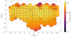 |
Fig. 1. Logarithmic density, in Galactic coordinates, of all the sources from the BDBS/Gaia EDR3 matched catalogue. The colour is proportional to the number of stars in each bin. The bins have sizes of 2.26′×2.26′. The dashed box marks the region where we can use the extinction map derived by Simion et al. (2017). The red circle shows the location of the field centred on Baade’s window with a radius of 1°, analysed in Sect. 3. The black squares show the bulge fields examined in Sect. 4, each covering an area of 1 deg2. The blue-filled circles correspond to the known clusters in the field, taken from the catalogue of Harris (1996, 2010 edition). |
Uncertainties in Gaia EDR3 proper motions in the right ascension direction are shown as a function of the observed magnitude in the Gaia G band in Fig. 2 (the trend for the errors in proper motions in the declination direction is equivalent). We see how these values range from ∼20 μas yr−1 for bright sources (G ≲ 13), but then increase steeply with magnitudes, reaching ∼1 mas yr−1 at G = 20. Uncertainties in Gaia EDR3 parallaxes range from ∼20 μmas at G ≲ 13, to ∼1 mas for faint stars with G = 20.
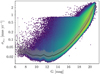 |
Fig. 2. Uncertainties in Gaia EDR3 proper motions in right ascension as a function of G magnitude for all the sources in the BDBS/Gaia EDR3 matched catalogue. The median value is shown with a solid black line, and the grey shaded area corresponds to the 1-sigma confidence interval, computed using the 16th and 84th percentiles of the distribution. |
3. Application to stars in Baade’s window
In this section, we focus only on stars in Baade’s Window, to describe the procedure we introduce to clean the observed CMDs based on Gaia EDR3 parallaxes and proper motions. Baade’s Window is one of the most observed and analysed bulge fields, because of its (relatively) low and uniform interstellar absorption (e.g., Holtzman et al. 1998). There are 3, 414, 177 sources in the BDBS/Gaia EDR3 catalogue within a radius of 1° from the centre of Baade’s Window, at (ℓ,b) = (+1.02° , − 3.92° ). This field is shown in Fig. 1 as a red circle. 2 039 126 of these stars have full astrometric solution from Gaia EDR33. We remove stars within 5′ from the centres of NGC 6522 and NGC 6528, the two known globular clusters in the field, and remain with a total of 2 002 241 sources with full astrometry from Gaia EDR3. These stars will be the main focus of this section.
3.1. Astrometric cleaning procedure
We correct Gaia EDR3 parallaxes by subtracting the estimated parallax zero-point ϖZP, following the approach described by Lindegren et al. (2021a). We apply the correction only to sources with Gaia G-band magnitudes 6 < G < 21, with 1.1 μm−1 < NU_EFF_USED_IN_ASTROMETRY < 1.9 μm−1 (for the sources with a 5-parameters solution from Gaia EDR3), and with 1.24 μm−1 < PSEUDOCOLOUR < 1.72 μm−1 (for the sources with a 6-parameters solution). For the sources outside these ranges, we assume ϖZP = 0. Here, NU_EFF_USED_IN_ASTROMETRY and PSEUDOCOLOUR are the effective wavenumbers used for the astrometric solution when Gaia DR2 photometry in the BP and RP bands was or was not available, respectively (Lindegren et al. 2021b). Gaia DR2 colours were used to calibrate the point spread function for the Gaia EDR3 astrometric solution. In case these were not available, a likely scenario for stars in the densest bulge fields, the astrometric pseudo-colour was estimated using the chromatic displacement of the image centroids. For the sample of stars in Baade’s Window, we find ϖZP ∈ [ − 0.08, 0.02] mas, with a median value of −0.025 mas. We remind the reader that the parallax zero-point should be subtracted from the observed parallaxes, therefore a mean negative value implies that, on average, stars are closer than the distance implied by the nominal value of their Gaia EDR3 parallax.
We then restrict our sample to the sources with reliable astrometric measurements from Gaia EDR3 and good photometry from BDBS in the g and i bands. The photometry was cleaned by selecting only stars that have median chi and sharp parameters residing within one standard deviation of the mean values in the original images. Furthermore, we restricted the sample to only include stars that did not have unusually high sky values relative to the local background on each image and were detected at least two times in each band. Further information about the quality flags is provided in Johnson et al. (2020). We also applied the following selection cuts on the Gaia EDR3 data:


where σμα* and σμδ are, respectively, the uncertainties on the proper motions in right ascension and declination, Δℓ and Δb are the means of the uncertainties in the distributions of proper motion in Galactic longitude and latitude in the field, respectively, computed from the 16 and the 84th percentiles of the distributions, and RUWE is the Gaia EDR3 renormalized unit weight error (see Lindegren et al. 2021b). The RUWE is the square-root of the reduced chi-square of the astrometric fit, and a large value is an indication of a bad determination of the astrometry of the star. Possible causes for a large value of RUWE include binarity, variability, and instrumental problems (Belokurov et al. 2020). A subset of 1 289 972 stars (∼64%) satisfies the criteria listed in Eqs. (1)–(5) and the cuts in BDBS photometry. The dereddened BDBS CMD for these sources, created using the reddening map by Simion et al. (2017), is shown in Fig. 3. We can see a well-defined RC at i0 ∼ 15, the MSTO region at i0 ∼ 17.6, a blue sequence at (g − i)0 ∼ 0 extending up to i0 ∼ 12 caused by foreground main sequence stars, and the population of putative ’blue loop’ stars at i0 ∼ 12, (g − i)0 ∼ 0.5 identified by Saha et al. (2019) in the same bulge field (see their Fig. 15).
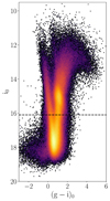 |
Fig. 3. Observed dereddened CMD for all the ∼1.3 × 10⁶ sources in Baade’s window, passing the quality cuts on the Gaia EDR3 astrometry and BDBS photometry. The horizontal dashed line marks the cut at i0 = i0, max − 3σi = 16.1 which we employ at the end of Sect. 3 to remove the MSTO and compute the ratio of blue to red stars in the field. |
To verify that the astrometric cuts do not introduce a bias in the CMDs, we inspect the CMD comprising the sources which do not satisfy the Gaia cuts in Eqs. (1)–(5). We find that the sources excluded are on average fainter and occupy unexpected regions of the HR diagram, such as the cloud at (g − i)0 ∼ −1 and i0 ∼ 18.5, and a plume at (g − i)0 ∼ 3 and i0 ∼ 15.5. The rest of the CMD is covered uniformly, allowing us to conclude that the cuts on proper motion do not significantly bias our results.
Even if Gaia EDR3 parallaxes are not precise and accurate enough to provide reliable distances to individual stars in the bulge (and in general beyond a few kpc from the Sun), they can be used to remove obvious foreground stars, which might otherwise contaminate our selection of bulge members. We define as ϖ-foreground stars all the sources satisfying:

and:

The first condition4 selects all the stars with estimated heliocentric distances within 5 kpc, while the second selection ensures that we consider only the stars with uncertainties small enough that an accurate distance can be determined by inverting the observed Gaia parallax (see Bailer-Jones 2015). For relative errors in parallax above ∼20%, the inverse of the observed parallax is a biased estimator for the distance of a star, and a Bayesian approach involving the use of prior probabilities on the distance of a star should be implemented (e.g., Bailer-Jones et al. 2018, 2021; Luri et al. 2018).
The observed CMD for the ∼7.7 × 10⁴ ϖ-foreground stars is shown in the left panel of Fig. 4. A well-defined blue sequence is observed centred at (g − i)0 ∼ 0, which is composed of nearby disk stars. A population of nearby bright giant stars is also clearly visible at (g − i)0 ∼ 1. The middle panel of Fig. 4 shows instead the observed CMD for the ϖ-background sources, defined as the original sample of stars minus the ϖ-foreground objects. This sample consists of ∼1.2 × 10⁶ stars. We can see how the foreground blue disk population is largely suppressed, but it is still evident at fainter magnitudes i0 ≳ 14.5 and (g − i)0 ∼ 0.5. These stars are possible foreground contaminants, which are not classified as such because of the large uncertainties in parallax due to their faintness (see Eq. (7)). Nevertheless, we note how almost all of the bright blue sources disappear when applying the cuts in parallax, including the bright “blue loop” population claimed by Saha et al. (2019), as already shown in Rich et al. (2020). The absence of blue loop stars in the CMDs will be further discussed in Sect. 3.2.
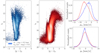 |
Fig. 4. Astrometric cleaning procedure using Gaia parallaxes. Left: dereddened BDBS CMD for all the ϖ-foreground stars in Baade’s window, defined as the sources with (ϖ−ϖZP) > 0.2 mas and σϖ/(ϖ−ϖZP) < 0.2. Middle: BDBS CMD for the ϖ-background sources. Right: distribution of proper motions in Galactic longitude (top) and latitude (bottom) for ϖ-foreground (blue) and ϖ-background (red) stars. The vertical dashed line corresponds to the cut in μℓ* employed by Clarkson et al. (2008) to select bulge members. |
Given the presence of a faint foreground population which is not easily removed using Gaia EDR3 parallaxes only, we rely on the more precise Gaia EDR3 proper motions, which allow us to further clean the observed CMD to a larger volume. Proper motions in Galactic coordinates μℓ* and μb are shown in the right-most panels of Fig. 4, in blue and red for the ϖ-foreground and ϖ-background sources, respectively. As already discussed in e.g., Kuijken & Rich (2002), Clarkson et al. (2008), Calamida et al. (2014), Bernard et al. (2018), Terry et al. (2020), μℓ* can be used to distinguish efficiently between foreground stars and bulge stars, even if there is a clear overlap between the distributions, at μℓ* ∼ −5 mas yr−1. A bump in the red distribution is also evident at μℓ* ∼ −2 mas yr−1, due to the contamination by foreground objects. The dashed vertical line at μℓ* = −2 mas yr−1 corresponds to the threshold value used by Clarkson et al. (2008) to isolate bulge members. The distributions in proper motions along Galactic latitude μb are instead more similar, even if for ϖ-foreground stars it peaks towards slightly lower (more negative) values. The power of proper motions to identify bulge stars is further shown in Fig. 5, where we present the CMDs for all the ϖ-background sources (left panel), colour-coded by the mean value of the proper motion in Galactic longitude and latitude (middle and right panels, respectively). From these plots, it is clear that foreground stars belonging to the blue disk sequence have on average higher values of μℓ* and lower values of μb. Figure 6 further shows the power of the proper motion in Galactic longitude to distinguish between blue and red stars. Here, we plot μℓ* as a function of the extinction-corrected colour (g − i)0. The red line corresponds to the median value of proper motion for each colour bin, and the red shaded region is computed from the 16th and 84th percentiles of the distribution in each bin. We observe a clear increase in the median value of μℓ* for (g − i)0 ∼ 0.5, corresponding to blue stars. The value for redder stars then reaches a plateau for μℓ* ∼ −6.5 mas yr−1.
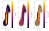 |
Fig. 5. Left: de-reddened CMD for all the ϖ-background sources in Baade’s Window, cleaned from foreground contaminants using Gaia EDR3 parallaxes. Colour is proportional to the logarithm of the density of sources. Middle: same CMD, colour-coded by the mean value of the proper motion in Galactic longitude. Right: same CMD, colour-coded by the mean value of the proper motion in Galactic latitude. To compare the proper motion values to their typical uncertainty in Gaia EDR3 (see Fig. 2), we note that i0 = 17 corresponds roughly to G = 18.5. |
Instead of using a single value of μℓ* for distinguishing between the two populations, we fitted the two-dimensional distribution in (μℓ*, μb) for the ϖ-background stars using a Gaussian Mixture Model (GMM) with two components, using the SKLEARN implementation (Pedregosa et al. 2011)5. We initialize one Gaussian to the mean proper motion we obtain for giant stars only, defined as background stars with i0 ≤ 15.5 (this cut, as shown in the middle panel of Fig. 4, excludes the great majority of stars belonging to the blue foreground sequence). The other Gaussian is instead initialized to (μℓ*, μb) = (0, 0) mas yr−1. The parameters of the resulting best-fitting bivariate Gaussian distributions are presented in Table 1, and the distributions are shown in Fig. 7, with a red (blue) curve for bulge (foreground) stars. We define the bulge subset as the subset of stars with proper motions consistent with belonging to the red Gaussian (lower values of μℓ*), and the μ-foreground sample as the subset of sources with proper motions consistent with belonging to the blue Gaussian. We see that the mean value for the bulge Gaussian, shown with a black horizontal dashed line in Fig. 6, corresponds to the expected value for giant stars. We note that the proper motion dispersions measured for the bulge and disk components, reported in Table 1, are similar to those reported in HST studies for this and nearby fields, suggesting that Gaia proper motion uncertainties are not significantly impacting our measured dispersions.
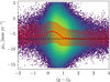 |
Fig. 6. Distribution of proper motion in Galactic longitude as a function of colour for the ϖ-background sources in Baade’s window. The red curve is the median value of μℓ* for each bin in (g − i)0, and the width of the red band is computed using the 16th and the 84th percentiles of the distribution of proper motions in each bin. The black dashed horizontal line corresponds to the mean of the Gaussian fitted to the distribution of the bulge stars. |
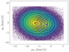 |
Fig. 7. Result of the GMM applied to the distribution of Galactic proper motions for ϖ-background stars in Baade’s window. The red and blue bivariate Gaussian distributions correspond to the bulge and to the μ-foreground population, respectively. The black curve is the sum of the two Gaussian distributions, and the crosses mark the position of the mean of the distributions. The parameters of the two distributions are summarized in Table 1. |
To further clean the CMDs and reduce the contamination from foreground stars, we can then assign to each star a weight equal to its probability of belonging to the bulge, according to the Gaia EDR3 proper motions:

Here, we use 𝒩(x, y) to indicate a bivariate Gaussian distribution, evaluated in the point (x, y). Figure 8 shows the observed CMD for all the ϖ-background stars, colour-coded by wbulge. We can clearly see that stars belonging to the blue sequence have lower probability to belong to the bulge given their proper motions (as expected from Fig. 5).
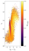 |
Fig. 8. De-reddened CMD for all the ϖ-background sources in Baade’s Window, colour-coded by the probability of bulge membership according to Gaia EDR3 proper motions (Eq. (8)). |
We now use wbulge to weight each star by its probability of belonging to the Galactic bulge, according to its Gaia EDR3 proper motions. Figure 9 summarizes the step used to clean the CMDs using Gaia EDR3 parallaxes and proper motions. The left panel shows the CMD for all the ∼1.3 × 10⁶ sources surviving the Gaia EDR3 and BDBS quality cuts. The middle panel shows the distribution of the ϖ-background sources surviving the Gaia EDR3 parallax cuts, while in the right panel we plot the same CMD for bulge stars, where each star is weighted by its probability wbulge of belonging kinematically to the Galactic bulge. We find a total of 8.8 × 10⁵ stars to be consistent with belonging to the Galactic bulge, according to their parallax and proper motions. We also note that all the bright blue stars are removed from the cleaned CMD, pointing to the fact that the claim of a strong constituency of very young stars in the bulge is not supported by the results presented here. The persistence of a faint blue sequence at (g − i)0 ∼ 0 proves that the GMM cleaning is still not perfect, as also evident from Fig. 7 and from the parameters of the Gaussian distributions listed in Table 1, which show a significant overlap between the proper motions of the two populations. In Appendix B we show that, when imposing much stricter cuts in proper motions to select bulge stars, μℓ* < −5 mas yr−1, this blue plume becomes less prominent, hinting towards the fact that this might be caused by foreground contaminants.
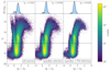 |
Fig. 9. Density plots illustrating the parallax and proper motion cleaning of the dereddend CMD for stars in Baade’s window. Left: all sources with reliable BDBS photometry and Gaia EDR3 astrometry. Middle: same as middle panel in Fig. 4, ϖ-background sources surviving the Gaia EDR3 parallax cuts. Right: subset of the ∼3.3 × 10⁵ sources with Gaia EDR3 proper motions consistent with a bulge membership, according to the GMM. The blue histograms above the CMDs represent the corresponding normalized distributions of (g − i)0 for stars brighter than i0, max − 3σi = 16.1 (shown as a horizontal dashed line in all three plots). The dashed curves correspond to the two fitted Gaussian distributions, and the black curve to their sum. The corresponding value of fB (the ratio between blue and red stars) is reported in each panel. |
To quantify the maximum contamination from the foreground population in the clean bulge CMDs, we define the following estimator:
![$$ \begin{aligned} f_\mathrm{cont} = \frac{{\displaystyle \int } \min \Bigl [\mathcal{N} _\mathrm{bulge} (\mu _{\ell *}, \mu _b), \mathcal{N} _\mathrm \mu -foreground (\mu _{\ell *}, \mu _b)\Bigr ]d\mu _{\ell *} d\mu _b}{{\displaystyle \int } \mathcal{N} _\mathrm{bulge} (\mu _{\ell *}, \mu _b) d\mu _{\ell *} d\mu _b} \ . \end{aligned} $$](/articles/aa/full_html/2022/08/aa43921-22/aa43921-22-eq11.gif)
Here, the numerator corresponds to the overlapping area of the red and blue Gaussian distributions in Galactic proper motions shown in Fig. 7, while the denominator is the area of the red Gaussian distribution. fcont is therefore a measure of the contamination to the clean bulge CMDs from stars with proper motions consistent with belonging to the foreground population. For stars in Baade’s window, we find fcont = 0.18. The contamination from bulge stars to the μ-foreground population is instead higher, ∼0.54, because of the smaller weight of the blue Gaussian with respect to the red one, implying a higher number of bulge stars compared to foreground disk stars in the field.
To further quantify the presence of blue stars in the bulge, we now limit our analysis to stars brighter than the MSTO. We estimate this as the maximum i0, max of the i0 distribution for i0 > 17 (to remove any possible contribution from the RC). We then fit a Gaussian distribution to this distribution, to estimate its standard deviation σi. With the further condition i0 ≤ i0, max − 3σi = 16.1, we are left with a sample of 427, 951 stars with full Gaia EDR3 astrometry. This cut is shown with a horizontal dashed line in Figs. 3 and 9. We quantify the ratio fB between the blue and the red sequence populations in the cleaned CMDs by fitting two Gaussian distributions to the distribution of (g − i)0. This is shown in the normalized histograms of Fig. 9, where we see how the local maximum at (g − i)0 ∼ 0.4 becomes less prominent with further cleaning, confirming its identification with the disk foreground population. By comparing the areas of the two distributions, we find a fraction of blue to red stars for the cleaned CMD of fB ≡ Nblue/Nred = 0.0437. We see how fB decreases from ∼18% for all the sources, to ∼8% when removing the foreground objects using Gaia EDR3 parallaxes (the ϖ-background sample), to ∼4% when adding the GMM proper motion cleaning (the bulge sample).
3.2. Location of the Blue Loop according to isochrones
As an additional demonstration, the top panel in Fig. 10 shows a sample of MIST isochrones (Dotter 2016) overplotted on a clean bulge BDBS CMD in Baade’s Window. The models are converted to the PanSTARRS photometry system to match the calibration of BDBS (Johnson et al. 2020), assume Solar composition, and span ages from 0.05 to 15 Gyr. To compute absolute magnitudes Mi0 we assume a distance modulus of 14.57, corresponding to a helio-centric distance of 8 kpc for all the stars. The chosen value for the distance corresponds to the mean distance of the RC sample in this field, as determined by Johnson et al. (2022), using BDBS data.
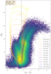 |
Fig. 10. Top: a selection of MIST isochrones adopting solar composition overlaid on BDBS photometry in Baade’s window, after the parallax and proper motion cleaning. The absolute magnitude in the i band Mi0 is computed assuming a fiducial distance of 8 kpc for all the stars. |
When the theoretical and observed MSTO regions align in the top panel of Fig. 10, it is evident that the stars purported to be blue-loop stars by Saha et al. (2019), observed at (g − i)0 ∼ 0.5, i0 ∼ 12, are not consistent with the location of the blue-loop feature predicted by the isochrones. The theoretical blue-loop is much brighter than the bulge RGB and falls in a region of the cleaned CMD that does not show any stars. This inconsistency persists in the same direction regardless of the composition assumed in the isochrones (over the range [Fe/H] = −1.8 through +0.5). This morphological difference is hence not explainable by inaccurate metallicity assumptions, nor could it be explained by observational issues that cause systematic offsets. As shown in Rich et al. (2020), these putative blue loop stars are foreground thin disk stars.
It is noteworthy that the purported blue-loop feature disappears entirely as better selection criteria are introduced into the cleaning procedure. Furthermore, any theoretical blue-loop that intersects the observed stars reported in Saha et al. (2019) requires a population < 250 Myr in age, and the cleaned CMD strongly rules out such a young main-sequence turn-off. Finally, we remind the reader that the position of the overdensity corresponding to the MSTO is highly affected by Gaia EDR3 incompleteness at the faint end, explaining the mismatch between the theoretical isochrones for ages ≳8 Gyr and the overdensity at Mi0 ∼ 3.2 in BDBS data.
4. Application to different bulge fields
In this section, we apply the methodology introduced and discussed in Sect. 3 to the 127 southern bulge fields shown with black squares in Fig. 1. The centres of these fields span a range in Galactic coordinates |ℓ| ≤ 9°, −9° ≤b ≤ −3°, each covering an area of 1 deg2. We remove the field at (ℓ,b) = (7° , − 8° ) and those at ℓ ≥ 5°, b = −9° because of the absence (or scarcity) of sources in the BDBS footprint. As mentioned in Sect. 2, the choice of the fields is driven by the range of applicability of the Simion et al. (2017) extinction map, which is valid for sources in the VVV footprint, with |ℓ| ≤ 10°, b ≥ −10°.
For each field, we remove all the sources within 5 arcmin from the centres of known clusters from Harris (1996, 2010 edition), and we apply the quality cuts on Gaia EDR3 astrometry and BDBS photometry discussed in Sect. 3, Eqs. (1) through (5). Then, we remove the ϖ-foreground sources, defined as those with precise parallaxes (corrected for the zero-point) consistent with the star being closer than 5 kpc from the Sun (see Eqs. (6) and (7)). We then use the GMM to fit the distribution in Galactic proper motions with two bivariate Gaussian distributions, for which we assume that the one with lower (more negative) values of μℓ* corresponds to the bulge stars. In Appendix A we explore and discuss the possibility to fit a higher number of Gaussian components to the proper motion distributions. The kinematic weights for each field are then computed using Eq. 8. Finally, for each field, we estimate the fraction of blue to red stars, fitting Gaussian distributions to the distribution in colour for sources brighter than the MSTO.
5. Results and discussion
In this section, we present the results we obtain for the individual bulge fields, following the approach discussed in Sect. 4.
5.1. Clean colour-magnitude diagrams
The clean CMDs for bulge stars in all the fields, obtained weighting their contribution by the corresponding value of wbulge, are presented in Fig. 11. The plots are presented following the arrangement of the fields shown in Fig. 1, so that each column corresponds to a constant value of the Galactic longitude ℓ (increasing from right to left), and each row to a constant value of the Galactic latitude b (increasing from bottom to top). The increase in Galactic longitude and latitude in each subsequent field centre is 1°. Similarly, in Fig. 12, we show the CMDs for all the foreground stars in each field, defined as the combined sample of sources satisfying Eqs. (6) and (7), and of ϖ-background stars weighted by 1 − wbulge (so the combination of the ϖ-foreground and the μ-foreground samples). The difference between Figs. 11 and 12 is most evident for the fields closer to the Galactic plane, where the RC is almost absent for the foreground stars, except along the bulge minor axis.
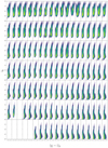 |
Fig. 11. Extinction-corrected and foreground-cleaned bulge CMDs for Galactic fields with |ℓ| ≤ 9° (rows), −9° ≤b ≤ −3° (columns), with a step of 1°. Each field contains all the sources within a square of 1 deg2. Galactic longitude ℓ increases towards the left of the plot, so that the plot in the top left corresponds to (ℓ,b) = (9° , − 3° ), and the one in the bottom right to (ℓ,b) = (−9° , − 9° ), as shown by the black circles in Fig. 1. |
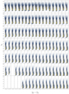 |
Fig. 12. Same as Fig. 11, but showing only the foreground sources in each field (selected using both Gaia EDR3 parallaxes and proper motions). |
We emphasize again that, because of the significant overlap between the two distributions in proper motions, there is a significant contamination from foreground stars in the bulge fields, as hinted by the presence of a sequence of blue stars. To quantify this possible contamination, we compute fcont using Eq. (9) for each bulge field. The result of this is shown in the first panel of Fig. 13. We find that fcont ∼ 20% at lower latitudes, and decreases to ∼10% at further away from the Galactic plane. A clear asymmetry in Galactic longitude, corresponding to the location of the near-side of the bar, is evident at ℓ > 0°.
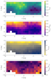 |
Fig. 13. First row: maximum contamination to the bulge CMDs from stars with proper motions consistent with belonging to the foreground population. Second row: ratio of foreground to background stars. Third row: maximum of the i0 distribution (for i0 > 17). Fourth Row: ratio of blue to red stars, when only stars with i0 ≤ i0, max − 3σi are considered. All the plots are shown as a function of Galactic coordinates, for the bulge fields shown in Fig. 1. |
In the second panel of Fig. 13 we show the ratio of the number of foreground to bulge stars in each field. We see how this varies from ∼25% for the fields further away from the Galactic plane, and increases to ∼50% at lower absolute values of Galactic latitude, where the density of stars in both the stellar disk and the bulge increases. We find this ratio to correlate strongly with the value of fcont.
In the third panel of Fig. 13, we plot i0, max, defined as the maximum of the i0 distribution in each field for i0 > 17, as a function of Galactic coordinates. The i0 > 17 cut is needed to ensure that the maximum of the distribution corresponds to the region of the MSTO, and to remove the possible contamination from the RC, which is particularly prominent in the fields close to the plane, especially at (ℓ,b) = (−3° , − 3° ). The shift in i0, max is due to two main effects: the presence of dust features, which redden the observed magnitudes and lower the maximum absolute magnitude observable in each field, and the Gaia completeness, which is a strong function of Galactic latitude and crowding of the field (see Boubert & Everall 2020). Also, the presence of the near-side of the bar induces a dependence on ℓ, contributing to a decrease in the value of i0, max at positive values of the Galactic longitude.
We then quantify the ratio of blue to red stars in each bulge field, as previously explained in Sect. 3 for stars in Baade’s Window. We select only stars with i0 ≤ i0, max − 3σi to minimize the contribution from the region around the MSTO, where red giants and nearby disk stars have a similar colour. The bottom panel in Fig. 13 shows the ratio between the areas of the blue and red fitted Gaussian distributions for the bulge fields explored in this work. We see that these values range from ∼2.6% for the fields along the bulge major axis, to ∼40% further away from the Galactic plane. We note that the bulge population drops dramatically with increasing distance from the Galactic plane, therefore a lower value of Nblue/Nred at low latitudes should not be regarded as an estimate of the contamination from the stellar disk. At lower latitudes, the prominence of the RC (as shown in Fig. 11) results in lower values of Nblue/Nred, while on the other hand, at higher latitudes, the fraction of red stars is lower, resulting in higher values of Nblue/Nred. Here we stress that Nblue/Nred is computed only for the ϖ-background stars (that is, after removing foreground stars using Gaia parallaxes), and therefore the contribution from blue disk stars brighter than the MSTO is further suppressed. This explains the observed anti-correlation between the values of Nfore/Nbkg and Nblue/Nred, shown when comparing the second and fourth panel in Fig. 13. A further discussion on the population of blue stars in the fields and their kinematics is provided in Sect. 5.3.
5.2. Kinematic Transverse Maps
We can use the results of the GMM applied to Gaia EDR3 proper motions to investigate the transverse kinematics of stars in the different bulge fields explored in this work. Following the works of Clarke et al. (2019), Sanders et al. (2019) using VVV and Gaia DR2 data, we quantify the bulge kinematics using the mean proper motions of the bulge stars ⟨μℓ*⟩, ⟨μb⟩, the corresponding dispersions σμℓ*, σμb, the dispersion ratio σμℓ*/σμb, and the correlation coefficient between the proper motions ρ(μℓ*, μb). These quantities are presented in Fig. 14 for all the bulge fields shown in Fig. 1. For an easier comparison, we use the same colours and a similar range as in Fig. 10 of Clarke et al. (2019). The first two panels show the projected mean rotation of the bulge stars along ℓ and b, respectively, and are offset because of the tangential reflex motion of the Sun (see Reid & Brunthaler 2004). The third and fourth panel, showing the proper motion dispersions, reach a well-defined maximum near the Galactic plane along the minor axis, due to the potential well of the bulge. Also, the observed asymmetries with the Galactic longitude are due to the inclination of the bar, with dispersions being generally smaller (larger) at ℓ < 0 (ℓ > 0), when the bar is further away from (closer to) the Sun. The fifth panel shows the dispersion ratio, which is ∼1 along the bulge minor axis, and reaches higher values ∼1.2 near the Galactic plane. The dipole pattern in the correlation between the proper motion components (which becomes a quadrupole pattern when one has access to the Northern Galactic bulge) shows a radial alignment towards the Galactic Centre, and it reaches its maximum amplitudes around b ∼ −6°, due to the triaxial shape of the bulge.
 |
Fig. 14. Kinematic transverse maps derived from the parameters of the Gaussian distribution of the bulge members fitted to Gaia EDR3 proper motions, for the same bulge fields shown in Fig. 1. From top to bottom, we show the mean proper motions in Galactic longitude and latitude, the proper motion dispersions in Galactic longitude and latitude, the dispersion ratio, and the correlation between the proper motions. |
In general, we find a very good agreement with the results presented in Clarke et al. (2019), Sanders et al. (2019), both in terms of the VIRAC data (Smith et al. 2018), and of the made-to-measure (M2M) model (Portail et al. 2017; Clarke et al. 2019). The magnitude of the dispersions, dispersion ratio, and correlation is also consistent with the study of Kozłowski et al. (2006) in the vicinity of Baade’s window. This proves the convergence of the GMM to the expected values, further validating the approach introduced in this paper, and it confirms the kinematic results with the more precise Gaia EDR3 astrometry.
5.3. Blue stars in the bulge
The fourth panel of Fig. 13 shows that the ratio between blue and red stars in the bulge fields considered in this work is typically around ∼3% near the Galactic plane, increasing towards higher absolute Galactic latitudes to ∼20%. This blue population is clearly visible in the cleaned bulge CMDS shown in Fig. 11, where it is most evident in the fields at b ≥ −4° where it clearly separates from the red giant branch.
We now investigate the kinematics of blue and red stars, to understand whether blue stars belong to the bulge population. As explained in Sect. 5.1, we only consider stars with i0 ≤ i0, max − 3σi. We then fit two Gaussian distributions to the resulting distribution in (g − i)0. Following Eq. (8), we compute the probability of each star to belong to the blue population as:
We can then isolate blue stars by weighting each star in the ϖ-background sample by the probability wbluewbulge, and red stars weighting by the probability (1 − wblue)wbulge. The first four panels of Fig. 15 show the mean proper motions and the proper motion dispersion in Galactic longitude for blue and red stars. The last panel shows instead the difference between the mean proper motion in Galactic longitude between blue and red stars. In these plots we focus on μℓ* because it is the proper motion component that is more efficient at separating the bulge and the foreground populations. By comparing Figs. 13–15, we can see how the population of blue stars shows significantly different trends as a function of Galactic coordinates, with respect to the expected patterns for an X-shaped triaxial bulge (Clarke et al. 2019; Sanders et al. 2019). In particular, we can see how the mean proper motion along Galactic longitude increases with increasing Galactic latitude, which is the opposite of what is predicted for bulge stars. The red stars, on the other hand, show kinematics consistent with what shown in Fig. 13.
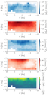 |
Fig. 15. From top to bottom, we show the mean proper motion in ℓ for blue stars, the mean proper motion in ℓ for red stars, the dispersion in proper motions in ℓ for blue stars, the dispersion in proper motions in ℓ for red stars, and the difference between the mean proper motions in ℓ for blue and red stars. All the plots are shown as a function of Galactic coordinates, for the southern bulge fields shown in Fig. 1. |
As a further check, in Appendix B we show that the faint blue sequence visible in Fig. 11, especially in the fields closer to the Galactic plane, is highly suppressed when imposing the much stricter cut μℓ* < −5 mas yr−1. Together with Fig. 15, this is a strong indication that this peculiar feature is likely to be caused by faint foreground disk stars, whose parallax is too imprecise to have a distance determination from Gaia EDR3, and whose proper motions lay in the overlapping region between the bulge and foreground distributions.
5.4. Estimating the age of the dominant population of stars
As a proof of concept, in this Section we derive age estimates for the bulge field in Baade’s window, showing the importance of a clean astrometric foreground removal to infer the overall distribution of ages of stars in the Milky Way bulge. In Fig. 16 we show the distribution of absolute magnitudes for sources with (g − i)0 ≥ 0.8, to exclude the contamination from blue stars and from the MSTO. Following Surot et al. (2019a), we fitted the distribution with the sum of a fourth-order polynomial (for the background density) and three Gaussian distributions. While the third Gaussian is not needed to explain the observed trend, the RC (purple curve) and the red giant branch (RGB) bump (blue curve) are clearly visible in the luminosity function. We find that the RC has a mean magnitude Mi0 = 0.61, with a standard deviation of 0.31. The RGB bump is instead observed at Mi0 = 1.34, with a standard deviation of 0.25.
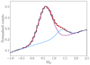 |
Fig. 16. Gaussian fits to the absolute magnitude distribution for sources in Baade’s window with (g − i)0 ≥ 0.8 (dash-dotted vertical line in Fig. 10). The purple curve corresponds to the RC, while the blue one to the RGB bump. Absolute magnitudes are computed assuming a mean distance of 8 kpc for all the stars. |
Since the absolute magnitudes are not calibrated, but they are just computed assuming a mean distance for all the stars corresponding to the mean distance of the RC stars in the field (Johnson et al. 2022), we cannot directly compare their location to the theoretical values predicted by the MIST isochrones. For this reason, here we discuss the use of the distance from the RGB bump to the RC as an age indicator for the dominant stellar population in a given bulge field. We derive the location of the RGB bump and of the RC in MIST isochrones of different ages and metallicities, by visually inspecting the HR diagrams. Figure 17 shows the difference of the absolute magnitude in the i band for the RGB bump and RC, ΔRGBB − RC, as a function of the age of the population. The three chosen values of [Fe/H] and [α/Fe] correspond to the adopted values in Baade’s window, and in the fields at (ℓ,b) = (0° , − 6° ) and (ℓ,b) = (+5° , − 8° ) explored in Appendix C. The coloured lines correspond to linear fits to the data points:
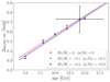 |
Fig. 17. Distance between the RGB bump and the RC in the i band as a function of age for MIST isochrones of different metallicities and alpha abundances. The lines are linear fits to the theoretical points. The black dot, with its uncertainties, corresponds to the value obtained in this work for stars in Baade’s Window. |
where t is the age of the isochrone in Gyr. The fitted parameters a and b, together with their uncertainties, are provided in Table 2 for three values of metallicities and abundances. The three fits are consistent with each other, even if it is possible to observe a trend at a given age: isochrones with lower values of [Fe/H] (and higher values of [α/Fe]) show systematically lower values of the i-band magnitude distance between the RGB bump and the RC.
We can now use the relation between the age and the magnitude difference between the RGB bump and the RC to estimate the age of the dominant stellar population in Baade’s window. By inverting Eq. (11), given the fitted positions of the RGB bump and RC, we can estimate the ages as:
The corresponding uncertainty on the age can then be estimated using error propagation:
where σa and σb are the uncertainties on the parameters a and b, provided in Table 2, and  is the combined uncertainty on the locations of the RGB bump and RC, which we assume σRGBB = σRC = 0.1 mag.
Using Eqs. (12) and (13), and the values of the RGB bump and RC derived from the Gaussian fits, we obtain ΔRGBB − RC = 0.73 ± 0.14, and therefore a mean age for stars in Baade’s window of (14.13 ± 3.92) Gyr. This value is shown with a black dot in Fig. 17. This age estimate, despite the large uncertainties, points to the picture of a predominantly old bulge, and is consistent with other measurements in the same field (e.g., Zoccali et al. 2003; Clarkson et al. 2008; Schultheis et al. 2017).
This is further confirmed by Fig. 18, where in the top panel we show a selection of MIST isochrones for [Fe/H] = 0 and [α/Fe] = 0. If we make the assumption that the mean age of the stellar population of the field is 10 Gyr, and that it has the same metallicity and alpha abundances as the Sun, then the fitted standard deviation of 0.25 of the Gaussian distribution corresponding to the RGB bump in Baade’s window can give us an approximate estimate of the minimum age of the stars in the field. By looking at the theoretical isochrones, we see how the observed uncertainty is marginally consistent with the location of the RGB bump for a population of 6 Gyr, while stellar ages ≤5 Gyr are excluded at 1 sigma level. The bottom panel of Fig. 18 shows instead MIST isochrones for [Fe/H] = +0.3 and [α/Fe] = 0. If we now assume that the bulk of the population is best described by the MIST isochrone with t = 10 Gyr and [Fe/H] = 0, then we see how a variation of +0.3 dex in metallicity extends the range of ages compatible with the observations, and only ages < 4 Gyr can be excluded at 1 sigma level.
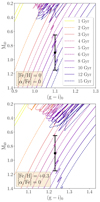 |
Fig. 18. Set of MIST isochrones for [Fe/H] = 0 and [α/Fe] = 0 (top panel), and [Fe/H] = +0.3 and [α/Fe] = 0 (bottom panel). The black point corresponds to the fitted value of the RGB bump in Baade’s window, assuming a mean age for the stars of 10 Gyr, and a mean solar metallicity. |
Because of the complex morphology of the Galactic bulge, this simplistic approach is not suited for fields at higher latitudes, where the X-shaped structure results into the overlapping along the line of sight of stellar populations at different distances. In Appendix C we further discuss this, showing an example from a more complex field at (ℓ,b) = (0° , − 6° ).
6. Summary and conclusions
In this analysis, we have demonstrated the power of using precise Gaia EDR3 astrometry to remove the vast majority of foreground star contamination brighter than the MSTO, and produce clean BDBS optical CMDs for stars in the bulge. No photometric information was used to isolate the bulge stars from the foreground population. We analysed 127 different fields in the southern Galactic bulge, spanning ℓ ≤ 9.5° and −9.5° ≤b ≤ −2.5°. Gaia EDR3 parallaxes were used to remove obvious foreground stars with precise parallaxes consistent with the stars being within a few kpc from the Sun. Additionally, we show how Gaia EDR3 proper motions can be further used to separate foreground stars from the bulge population. We used a GMM algorithm to fit two bivariate Gaussian distributions to the distribution of proper motions in Galactic longitude and latitude, which we then employed to assign to each star a probability to belong to the bulge according to its measured astrometry. We can summarize the main results of this paper as follows:
-
We produced extinction-corrected and foreground-cleaned bulge CMDs for 127 individual fields in the southern Galactic bulge. The astrometric cleaning procedure removes the majority of the blue stars from each field, while retaining the population of red giants.
-
The contamination from foreground stars with proper motions consistent with the bulge population in the CMDs is, at maximum, at a level of ∼20% near the plane, with values ∼10% at higher absolute values of the Galactic latitude.
-
The overall ratio of foreground to background stars is found to be maximum for the fields at lower absolute Galactic latitudes, where it can be as high as ∼50%. This value decreases further away from the plane, reaching ∼25%.
-
We produced kinematic transverse maps, recovering the expected kinematic patterns caused by the orientation of the bar and the morphological structure of the Milky Way bulge. The proper motion dispersions peak at ∼2.8 mas yr−1 near the plane because of the potential well of the Milky Way bulge, and decrease with increasing distance from the plane. The asymmetry of the dispersions with Galactic longitude is caused by the orientation of the bar. The radially-aligned quadrupole pattern observed in the proper motion correlation is a direct consequence of the X-shaped structure of the bulge.
-
We quantified the fraction of blue to red bulge stars brighter than the MSTO, finding this to be around 3% closer to the plane, and increasing to ∼20% for the fields further away from the plane. This value is driven by the prominence of the RC in the CMDs of the fields at lower latitudes, and it should not be interpreted as an estimate of the residual contamination from stars belonging to the stellar disk.
-
The population of blue stars visible especially in the fields closer to the Galactic plane is likely to be a residual foreground population. This particularly evident when investigating the kinematics of the red and blue stars in each field, and when applying more severe cuts in proper motions to isolate a pure bulge sample.
-
The application of Gaia EDR3 astrometric cleaning clearly shows that no widespread population of young He-burning blue loop stars is present across the bulge, and places strong limits on stars younger than 2 Gyr.
-
We have derived a tight linear relation between the difference of the i-band magnitudes of the RGB bump and of the RC as a function of age, constructed from a set of MIST isochrones for different values of [Fe/H] and [α/Fe]. We have used this relation to derive a mean age of (14.13 ± 3.92) Gyr for stars in Baade’s window. If we assume that the mean age of the population is 10 Gyr (Schultheis et al. 2017), then contribution from stars with ages < 6 Gyr (< 4 Gyr) can be excluded at 1 sigma level for a mean metallicity [Fe/H] = 0 ([Fe/H]= + 0.3). The application of this method to fields at higher Galactic latitudes, where projection effects due to the morphology of the Galactic bulge become important, requires further work on the modelling of the populations.
Most of the interesting star formation history of the bulge, and the origin of the bar, will very likely require ages of 1−2 Gyr precision for stars older than 5 Gyr. These efforts offer the possibility of constraining whether the bar formed substantially later than the thick disk, and potentially whether the halo population is older still. With advanced kinematic models of the bulge and the derivation of photometric metallicities at the MSTO level (e.g., Brown et al. 2010), one can envision some significant advances in age constraints, especially in the outer bulge fields where crowding and reddening are less severe. Future improvements in the precision of parallaxes and proper motions may be of great value in this endeavour. The extended observational baseline of future Gaia data releases will result into a more precise and accurate determination of the astrometry of the stars, allowing us to refine the cleaning procedure and to lower the contamination from foreground objects. In particular, Gaia DR4 (DR5) will be based on 5.5 years (10 years) of data, and parallax precisions will improve by a factor of ∼1.33 (∼1.90) with respect to Gaia EDR3. For proper motions instead, the improvement will be ∼2.4 and ∼7.1 for Gaia DR4 and Gaia DR5, respectively, compared to Gaia EDR36. Looking at the future, the proposed space mission GaiaNIR, an all-sky near-infrared survey, will allow probing the central region of our Galaxy, providing photometry and astrometry for more than 10 billion stars (Hobbs et al. 2016; Høg 2021). Proper motions (parallaxes) from Gaia NIR will be 10−20 ( ) times more precise than the final data release of Gaia, thanks to the improved baseline of 20 years (Hobbs et al. 2019). Gaia DR5 will also provide radial velocities for all sources brighter than the 16th magnitude in the Radial-Velocity Spectrometer (RVS) band. In addition, the advent of multi-object spectroscopic facilities such as MOONS (Gonzalez et al. 2020) and 4MOST (de Jong et al. 2012), will complement Gaia observations, providing spectra for million of stars in the bulge (Chiappini et al. 2019). The combined three-dimensional velocity will be essential to produce a precise foreground subtraction for the brightest stars, allowing the study of bulge CMDs to an unprecedented level of details.
In this work, we do not differentiate between sources with 5-parameter and 6-parameter solutions from Gaia EDR3 (Lindegren et al. 2021b) and we use the astrometric pseudo-colour, when available, only to estimate the parallax zero-point. With full astrometric solution, we refer to the complete determination of the 5 astrometric parameters: coordinates, parallax, and proper motions.
We also experiment using the extreme deconvolution algorithm (Bovy et al. 2011), which takes into account the full proper motion covariance matrix for each star, using the ASTROML implementation (Vanderplas et al. 2012). We find the results to be indistinguishable to those obtained using the simpler GMM, and therefore we decide to choose the latter, simpler method. This follows from the fact that the observed dispersion in proper motions is dominated by the intrinsic velocity dispersion of the stars, and not by the measurement uncertainties (see Fig. 2).
Acknowledgments
The authors thank the anonymous referee for their comments, which greatly improved the quality of this manuscript. T.M. thanks M. Rejkuba for interesting discussions. T.M. acknowledges an ESO Fellowship. M.J. was supported primarily by the Lasker Data Science Fellowship, awarded by the Space Telescope Science Institute. M.J. further acknowledges the Kavli Institute for Theoretical Physics at the University of California, Santa Barbara, whose collaborative residency program TRANSTAR21 was supported by the National Science Foundation under Grant No. NSF PHY-1748958. A.M.K. acknowledges support from grant AST-2009836 from the National Science Foundation. A.J.K.-H. gratefully acknowledges funding by the Deutsche Forschungsgemeinschaft (DFG, German Research Foundation) – Project-ID 138713538 – SFB 881 (“The Milky Way System”), subprojects A03, A05, A11. Data used in this paper comes from the Blanco DECam Survey Collaboration. This project used data obtained with the Dark Energy Camera (DECam), which was constructed by the Dark Energy Survey (DES) collaboration. Funding for the DES Projects has been provided by the U.S. Department of Energy, the U.S. National Science Foundation, the Ministry of Science and Education of Spain, the Science and Technology Facilities Council of the United Kingdom, the Higher Education Funding Council for England, the National Center for Supercomputing Applications at the University of Illinois at Urbana-Champaign, the Kavli Institute of Cosmological Physics at the University of Chicago, the Center for Cosmology and Astro-Particle Physics at the Ohio State University, the Mitchell Institute for Fundamental Physics and Astronomy at Texas A&M University, Financiadora de Estudos e Projetos, Fundaçõ Carlos Chagas Filho de Amparo á Pesquisa do Estado do Rio de Janeiro, Conselho Nacional de Desenvolvimento Científico e Tecnológico and the Ministério da Ciência, Tecnologia e Inovacão, the Deutsche Forschungsgemeinschaft, and the Collaborating Institutions in the Dark Energy Survey. The Collaborating Institutions are Argonne National Laboratory, the University of California at Santa Cruz, the University of Cambridge, Centro de Investigaciones Enérgeticas, Medioambientales y Tecnológicas-Madrid, the University of Chicago, University College London, the DES-Brazil Consortium, the University of Edinburgh, the Eidgenössische Technische Hochschule (ETH) Zürich, Fermi National Accelerator Laboratory, the University of Illinois at Urbana-Champaign, the Institut de Cióncies de l’Espai (IEEC/CSIC), the Institut de Física d’Altes Energies, Lawrence Berkeley National Laboratory, the Ludwig-Maximilians Universität München and the associated Excellence Cluster Universe, the University of Michigan, the National Optical Astronomy Observatory, the University of Nottingham, the Ohio State University, the OzDES Membership Consortium the University of Pennsylvania, the University of Portsmouth, SLAC National Accelerator Laboratory, Stanford University, the University of Sussex, and Texas A&M University. Based on observations at Cerro Tololo Inter-American Observatory (2013A-0529; 2014A-0480; PI: Rich), National Optical Astronomy Observatory, which is operated by the Association of Universities for Research in Astronomy (AURA) under a cooperative agreement with the National Science Foundation. This work has made use of data from the European Space Agency (ESA) mission Gaia (https://www.cosmos.esa.int/gaia), processed by the Gaia Data Processing and Analysis Consortium (DPAC, https://www.cosmos.esa.int/web/gaia/dpac/consortium). Funding for the DPAC has been provided by national institutions, in particular the institutions participating in the Gaia Multilateral Agreement. Software used: numpy (Harris et al. 2020), matplotlib (Hunter 2007), scipy (Virtanen et al. 2020), astropy (Astropy Collaboration 2013, 2018), scikit-learn (Pedregosa et al. 2011), pomegranate (Schreiber 2017), astroML (Vanderplas et al. 2012), TOPCAT (Taylor 2005, 2006).
References
- Arentsen, A., Starkenburg, E., Martin, N. F., et al. 2020, MNRAS, 491, L11 [Google Scholar]
- Astropy Collaboration (Robitaille, T. P., et al.) 2013, A&A, 558, A33 [NASA ADS] [CrossRef] [EDP Sciences] [Google Scholar]
- Astropy Collaboration (Price-Whelan, A. M., et al.) 2018, AJ, 156, 123 [Google Scholar]
- Babusiaux, C. 2016, PASA, 33 [CrossRef] [Google Scholar]
- Bailer-Jones, C. A. L. 2015, PASP, 127, 994 [Google Scholar]
- Bailer-Jones, C. A. L., Rybizki, J., Fouesneau, M., Mantelet, G., & Andrae, R. 2018, AJ, 156, 58 [Google Scholar]
- Bailer-Jones, C. A. L., Rybizki, J., Fouesneau, M., Demleitner, M., & Andrae, R. 2021, AJ, 161, 147 [Google Scholar]
- Barbuy, B., Chiappini, C., & Gerhard, O. 2018, ARA&A, 56, 223 [Google Scholar]
- Belokurov, V., Penoyre, Z., Oh, S., et al. 2020, MNRAS, 496, 1922 [Google Scholar]
- Bensby, T., Yee, J. C., Feltzing, S., et al. 2013, A&A, 549, A147 [NASA ADS] [CrossRef] [EDP Sciences] [Google Scholar]
- Bensby, T., Feltzing, S., Gould, A., et al. 2017, A&A, 605, A89 [NASA ADS] [CrossRef] [EDP Sciences] [Google Scholar]
- Bernard, E. J., Schultheis, M., Di Matteo, P., et al. 2018, MNRAS, 477, 3507 [CrossRef] [Google Scholar]
- Binney, J., Gerhard, O. E., Stark, A. A., Bally, J., & Uchida, K. I. 1991, MNRAS, 252, 210 [Google Scholar]
- Bland-Hawthorn, J., & Gerhard, O. 2016, ARA&A, 54, 529 [Google Scholar]
- Boubert, D., & Everall, A. 2020, MNRAS, 497, 4246 [NASA ADS] [CrossRef] [Google Scholar]
- Bovy, J., Hogg, D. W., & Roweis, S. T. 2011, Ann. Appl. Stat., 5, 1657 [Google Scholar]
- Brown, T. M., Sahu, K., Anderson, J., et al. 2010, ApJ, 725, L19 [NASA ADS] [CrossRef] [Google Scholar]
- Calamida, A., Sahu, K. C., Anderson, J., et al. 2014, ApJ, 790, 164 [NASA ADS] [CrossRef] [Google Scholar]
- Catchpole, R. M., Whitelock, P. A., Feast, M. W., et al. 2016, MNRAS, 455, 2216 [NASA ADS] [CrossRef] [Google Scholar]
- Chiappini, C., Minchev, I., Starkenburg, E., et al. 2019, The Messenger, 175, 30 [NASA ADS] [Google Scholar]
- Choi, J., Dotter, A., Conroy, C., et al. 2016, ApJ, 823, 102 [Google Scholar]
- Clarke, J. P., Wegg, C., Gerhard, O., et al. 2019, MNRAS, 489, 3519 [Google Scholar]
- Clarkson, W., Sahu, K., Anderson, J., et al. 2008, ApJ, 684, 1110 [NASA ADS] [CrossRef] [Google Scholar]
- Clarkson, W. I., Sahu, K. C., Anderson, J., et al. 2011, ApJ, 735, 37 [NASA ADS] [CrossRef] [Google Scholar]
- Clarkson, W. I., Calamida, A., Sahu, K. C., et al. 2018, ApJ, 858, 46 [NASA ADS] [CrossRef] [Google Scholar]
- de Jong, R. S., Bellido-Tirado, O., Chiappini, C., et al. 2012, in Ground-based and Airborne Instrumentation for Astronomy IV, eds. I. S. McLean, S. K. Ramsay, & H. Takami, SPIE Conf. Ser., 8446, 84460T [NASA ADS] [Google Scholar]
- Di Matteo, P., Gómez, A., Haywood, M., et al. 2015, A&A, 577, A1 [NASA ADS] [CrossRef] [EDP Sciences] [Google Scholar]
- Di Matteo, P., Fragkoudi, F., Khoperskov, S., et al. 2019, A&A, 628, A11 [NASA ADS] [CrossRef] [EDP Sciences] [Google Scholar]
- Dotter, A. 2016, ApJS, 222, 8 [Google Scholar]
- Erwin, P., Saglia, R. P., Fabricius, M., et al. 2015, MNRAS, 446, 4039 [Google Scholar]
- Erwin, P., Seth, A., Debattista, V. P., et al. 2021, MNRAS, 502, 2446 [NASA ADS] [CrossRef] [Google Scholar]
- Fragkoudi, F., Grand, R. J. J., Pakmor, R., et al. 2020, MNRAS, 494, 5936 [Google Scholar]
- Freeman, K., Ness, M., Wylie-de-Boer, E., et al. 2013, MNRAS, 428, 3660 [NASA ADS] [CrossRef] [Google Scholar]
- Gaia Collaboration (Prusti, T., et al.) 2016, A&A, 595, A1 [NASA ADS] [CrossRef] [EDP Sciences] [Google Scholar]
- Gaia Collaboration (Brown, A. G. A., et al.) 2021, A&A, 649, A1 [NASA ADS] [CrossRef] [EDP Sciences] [Google Scholar]
- Gilmore, G., Randich, S., Asplund, M., et al. 2012, The Messenger, 147, 25 [NASA ADS] [Google Scholar]
- Gonzalez, O. A., Zoccali, M., Vasquez, S., et al. 2015, A&A, 584, A46 [NASA ADS] [CrossRef] [EDP Sciences] [Google Scholar]
- Gonzalez, O. A., Mucciarelli, A., Origlia, L., et al. 2020, The Messenger, 180, 18 [NASA ADS] [Google Scholar]
- Gough-Kelly, S., Debattista, V. P., Clarkson, W. I., et al. 2022, MNRAS, 509, 4829 [Google Scholar]
- Harris, W. E. 1996, AJ, 112, 1487; 2010 edn: [arXiv:1012.3224] [Google Scholar]
- Harris, C. R., Millman, K. J., van der Walt, S. J., et al. 2020, Nature, 585, 357 [NASA ADS] [CrossRef] [Google Scholar]
- Hasselquist, S., Zasowski, G., Feuillet, D. K., et al. 2020, ApJ, 901, 109 [CrossRef] [Google Scholar]
- Haywood, M., Di Matteo, P., Snaith, O., & Calamida, A. 2016, A&A, 593, A82 [NASA ADS] [CrossRef] [EDP Sciences] [Google Scholar]
- Hobbs, D., Høg, E., Mora, A., et al. 2016, ArXiv e-prints [arXiv:1609.07325] [Google Scholar]
- Hobbs, D., Brown, A., Høg, E., et al. 2019, ArXiv e-prints [arXiv:1907.12535] [Google Scholar]
- Høg, E. 2021, ArXiv e-prints [arXiv:2107.07177] [Google Scholar]
- Holtzman, J. A., Watson, A. M., Baum, W. A., et al. 1998, AJ, 115, 1946 [Google Scholar]
- Horta, D., Schiavon, R. P., Mackereth, J. T., et al. 2021, MNRAS, 500, 1385 [Google Scholar]
- Hunter, J. D. 2007, Comput. Sci. Eng., 9, 90 [NASA ADS] [CrossRef] [Google Scholar]
- Johnson, C. I., Rich, R. M., Young, M. D., et al. 2020, MNRAS, 499, 2357 [NASA ADS] [CrossRef] [Google Scholar]
- Johnson, C. I., Rich, R. M., Simion, I. T., et al. 2022, MNRAS, 515, 1469 [NASA ADS] [CrossRef] [Google Scholar]
- Joyce, M., Johnson, C. I., Marchetti, T., et al. 2022, APJ, submitted ArXiv e-prints [arXiv:2205.07964] [Google Scholar]
- Kader, J. A., Pilachowski, C. A., Johnson, C. I., et al. 2022, ApJ, submitted ArXiv e-prints [arXiv: 2206.12817] [Google Scholar]
- Katz, D., Sartoretti, P., Cropper, M., et al. 2019, A&A, 622, A205 [NASA ADS] [CrossRef] [EDP Sciences] [Google Scholar]
- Kirby, E. N., Cohen, J. G., Guhathakurta, P., et al. 2013, ApJ, 779, 102 [Google Scholar]
- Kormendy, J., & Kennicutt, R. C., Jr 2004, ARA&A, 42, 603 [NASA ADS] [CrossRef] [Google Scholar]
- Kormendy, J., Drory, N., Bender, R., & Cornell, M. E. 2010, ApJ, 723, 54 [Google Scholar]
- Kozłowski, S., Woźniak, P. R., Mao, S., et al. 2006, MNRAS, 370, 435 [CrossRef] [Google Scholar]
- Kuijken, K., & Rich, R. M. 2002, AJ, 124, 2054 [NASA ADS] [CrossRef] [Google Scholar]
- Kunder, A., Koch, A., Rich, R. M., et al. 2012, AJ, 143, 57 [NASA ADS] [CrossRef] [Google Scholar]
- Kunder, A., Pérez-Villegas, A., Rich, R. M., et al. 2020, AJ, 159, 270 [NASA ADS] [CrossRef] [Google Scholar]
- Lim, D., Koch-Hansen, A. J., Chung, C., et al. 2021, A&A, 647, A34 [NASA ADS] [CrossRef] [EDP Sciences] [Google Scholar]
- Lindegren, L., Klioner, S. A., Hernández, J., et al. 2021a, A&A, 649, A2 [EDP Sciences] [Google Scholar]
- Lindegren, L., Bastian, U., Biermann, M., et al. 2021b, A&A, 649, A4 [EDP Sciences] [Google Scholar]
- Luri, X., Brown, A. G. A., Sarro, L. M., et al. 2018, A&A, 616, A9 [NASA ADS] [CrossRef] [EDP Sciences] [Google Scholar]
- Majewski, S. R., Schiavon, R. P., Frinchaboy, P. M., et al. 2017, AJ, 154, 94 [NASA ADS] [CrossRef] [Google Scholar]
- Massari, D., Koppelman, H. H., & Helmi, A. 2019, A&A, 630, L4 [NASA ADS] [CrossRef] [EDP Sciences] [Google Scholar]
- McWilliam, A., & Zoccali, M. 2010, ApJ, 724, 1491 [NASA ADS] [CrossRef] [Google Scholar]
- Minniti, D., Lucas, P. W., Emerson, J. P., et al. 2010, New Astron., 15, 433 [Google Scholar]
- Nataf, D. M., Udalski, A., Gould, A., Fouqué, P., & Stanek, K. Z. 2010, ApJ, 721, L28 [NASA ADS] [CrossRef] [Google Scholar]
- Nataf, D. M., Udalski, A., Gould, A., & Pinsonneault, M. H. 2011, ApJ, 730, 118 [NASA ADS] [CrossRef] [Google Scholar]
- Ness, M., Freeman, K., Athanassoula, E., et al. 2013, MNRAS, 432, 2092 [NASA ADS] [CrossRef] [Google Scholar]
- Pedregosa, F., Varoquaux, G., Gramfort, A., et al. 2011, J. Mach. Learn. Res., 12, 2825 [Google Scholar]
- Pietrukowicz, P., Udalski, A., Soszyński, I., et al. 2012, ApJ, 750, 169 [NASA ADS] [CrossRef] [Google Scholar]
- Pietrukowicz, P., Kozłowski, S., Skowron, J., et al. 2015, ApJ, 811, 113 [Google Scholar]
- Portail, M., Wegg, C., Gerhard, O., & Ness, M. 2017, MNRAS, 470, 1233 [NASA ADS] [CrossRef] [Google Scholar]
- Reid, M. J., & Brunthaler, A. 2004, ApJ, 616, 872 [Google Scholar]
- Renzini, A., & Fusi Pecci, F. 1988, ARA&A, 26, 199 [NASA ADS] [CrossRef] [Google Scholar]
- Renzini, A., Gennaro, M., Zoccali, M., et al. 2018, ApJ, 863, 16 [NASA ADS] [CrossRef] [Google Scholar]
- Rich, R. M. 2013, in The Galactic Bulge, eds. T. D. Oswalt, & G. Gilmore (Dordrecht: Springer Science+Business Media), 5, 271 [Google Scholar]
- Rich, R. M., Reitzel, D. B., Howard, C. D., & Zhao, H. 2007, ApJ, 658, L29 [NASA ADS] [CrossRef] [Google Scholar]
- Rich, R. M., Johnson, C. I., Young, M., et al. 2020, MNRAS, 499, 2340 [NASA ADS] [CrossRef] [Google Scholar]
- Riello, M., De Angeli, F., Evans, D. W., et al. 2021, A&A, 649, A3 [NASA ADS] [CrossRef] [EDP Sciences] [Google Scholar]
- Saha, A., Vivas, A. K., Olszewski, E. W., et al. 2019, ApJ, 874, 30 [NASA ADS] [CrossRef] [Google Scholar]
- Sanders, J. L., Smith, L., Evans, N. W., & Lucas, P. 2019, MNRAS, 487, 5188 [CrossRef] [Google Scholar]
- Savino, A., Koch, A., Prudil, Z., Kunder, A., & Smolec, R. 2020, A&A, 641, A96 [NASA ADS] [CrossRef] [EDP Sciences] [Google Scholar]
- Schreiber, J. 2017, ArXiv e-prints [arXiv:1711.00137] [Google Scholar]
- Schultheis, M., Rojas-Arriagada, A., García Pérez, A. E., et al. 2017, A&A, 600, A14 [NASA ADS] [CrossRef] [EDP Sciences] [Google Scholar]
- Seabroke, G. M., Fabricius, C., Teyssier, D., et al. 2021, A&A, 653, A160 [NASA ADS] [CrossRef] [EDP Sciences] [Google Scholar]
- Sestito, F., Longeard, N., Martin, N. F., et al. 2019, MNRAS, 484, 2166 [NASA ADS] [CrossRef] [Google Scholar]
- Shen, J., Rich, R. M., Kormendy, J., et al. 2010, ApJ, 720, L72 [NASA ADS] [CrossRef] [Google Scholar]
- Simion, I. T., Belokurov, V., Irwin, M., et al. 2017, MNRAS, 471, 4323 [NASA ADS] [CrossRef] [Google Scholar]
- Skrutskie, M. F., Cutri, R. M., Stiening, R., et al. 2006, AJ, 131, 1163 [NASA ADS] [CrossRef] [Google Scholar]
- Smith, L. C., Lucas, P. W., Kurtev, R., et al. 2018, MNRAS, 474, 1826 [Google Scholar]
- Soto, M., Rich, R. M., & Kuijken, K. 2007, ApJ, 665, L31 [NASA ADS] [CrossRef] [Google Scholar]
- Stanek, K. Z., Mateo, M., Udalski, A., et al. 1994, ApJ, 429, L73 [NASA ADS] [CrossRef] [Google Scholar]
- Stanek, K. Z., Udalski, A., Szymański, M., et al. 1997, ApJ, 477, 163 [NASA ADS] [CrossRef] [Google Scholar]
- Surot, F., Valenti, E., Hidalgo, S. L., et al. 2019a, A&A, 623, A168 [NASA ADS] [CrossRef] [EDP Sciences] [Google Scholar]
- Surot, F., Valenti, E., Hidalgo, S. L., et al. 2019b, A&A, 629, A1 [NASA ADS] [CrossRef] [EDP Sciences] [Google Scholar]
- Taylor, M. B. 2005, in Astronomical Data Analysis Software and Systems XIV, eds. P. Shopbell, M. Britton, & R. Ebert, ASP Conf. Ser., 347, 29 [Google Scholar]
- Taylor, M. B. 2006, in Astronomical Data Analysis Software and Systems XV, eds. C. Gabriel, C. Arviset, D. Ponz, & S. Enrique, ASP Conf. Ser., 351, 666 [Google Scholar]
- Terry, S. K., Barry, R. K., Bennett, D. P., et al. 2020, ApJ, 889, 126 [NASA ADS] [CrossRef] [Google Scholar]
- Udalski, A., Szymański, M. K., & Szymański, G. 2015, Acta Astron., 65, 1 [NASA ADS] [Google Scholar]
- Valenti, E., Zoccali, M., Renzini, A., et al. 2013, A&A, 559, A98 [NASA ADS] [CrossRef] [EDP Sciences] [Google Scholar]
- Vanderplas, J., Connolly, A., Ivezić, Ž., & Gray, A. 2012, in Conference on Intelligent Data Understanding (CIDU), 47 [CrossRef] [Google Scholar]
- Virtanen, P., Gommers, R., Oliphant, T. E., et al. 2020, Nat. Methods, 17, 261 [Google Scholar]
- Wegg, C., & Gerhard, O. 2013, MNRAS, 435, 1874 [Google Scholar]
- Weiland, J. L., Arendt, R. G., Berriman, G. B., et al. 1994, ApJ, 425, L81 [NASA ADS] [CrossRef] [Google Scholar]
- Zoccali, M., & Valenti, E. 2016, PASA, 33 [CrossRef] [Google Scholar]
- Zoccali, M., Renzini, A., Ortolani, S., et al. 2003, A&A, 399, 931 [NASA ADS] [CrossRef] [EDP Sciences] [Google Scholar]
- Zoccali, M., Gonzalez, O. A., Vasquez, S., et al. 2014, A&A, 562, A66 [NASA ADS] [CrossRef] [EDP Sciences] [Google Scholar]
Appendix A: Choosing the number of components for the Gaussian Mixture Model
We use the Bayesian information criterion (BIC) to select the optimal number of Gaussian components for the multivariate Gaussian distribution according to the GMM in each southern Galactic bulge field. Minimizing the BIC is a heuristic approach designed to select the model which best describes the data (maximizes the likelihood probability), but at the same time penalizes models with too many parameters (the total number of Gaussian distributions in this case), which might lead to overfitting. For each field, we remove ϖ-foreground stars using Gaia EDR3 parallaxes, and then we apply the GMM to the Gaia EDR3 proper motions, following the procedure outlined in Section 4. We explore a number of Gaussian components, ranging from 1 (a single Gaussian distribution) to 8. One of the Gaussian is initialized to the proper motion values obtained for giant stars, as discussed in Section 4, while all the others are initialized to (μℓ*, μb) = (0, 0) mas yr−1. We train the GMM 20 times for each chosen value of the number of Gaussian components nGMM, and we compute the BIC as the median of the individual values, to compensate for the effect of the intrinsic randomness of the GMM algorithm. We then select the number of Gaussian components which minimizes the value of the median BIC. The result is shown in Fig. A.1, for the Bulge fields discussed in Section 4. This plot shows that nGMM = 2 for fields further away from the Galactic plane, and increases to higher values towards b = 0. The value of nGMM is maximum near the plane, with nGMM = 8 along the bulge minor axis. We also observe an asymmetry at positive values of Galactic longitude due to the presence of the near-side of the Galactic bar. We note that, even for the fields in which nGMM = 8, the parameters of the Gaussian associated to the bulge stars (the red curve in Fig. 7) do not depend on the number of Gaussian components for the GMM, which affect only the μ-foreground distributions at μℓ* ∼ 0 mas yr−1. For this reason, in this work we choose to fit only two Gaussian components to the ϖ-background stars in the fields, to clearly isolate bulge and foreground stars. We refer to a future work the detailed investigation of the multiple population in proper motions for some fields, which might point towards the use of the precise Gaia EDR3 proper motions to decompose the density field and identify not only bulge stars, but also differentiate between other stellar populations. Finally, we want to stress that nGMM is not a precise determination of the exact number of individual populations in each field. A large value should be interpreted as an indication that a simple decomposition between bulge and foreground stars might be too simplistic, and it points to a higher complexity of the proper motion distribution in the field.
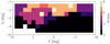 |
Fig. A.1. Number of Gaussian components in the GMM minimizing the median BIC, for the bulge fields shown in Fig. 1. |
Appendix B: Selecting the cleanest bulge CMDs
In this appendix we further clean the bulge CMDs shown in Fig. 11, reducing the completeness of the fields, but increasing their purity (see also Bernard et al. 2018; Terry et al. 2020). In Fig. B.1 we plot the bulge CMDs, selecting only sources with μℓ* < −5 mas yr−1. An individual CMD for stars in Baade’s window is shown in Fig. B.2. As evident from Fig. 7 and the first panel in Fig. 14, this cut in proper motion removes the great majority of stars with proper motions consistent with belonging to the disk foreground population, and maximizes the contribution from the bulge stars. The resulting CMDs show a less prominent blue sequence, especially for the fields closer to the disk plane. This hints to the fact that the leftover blue population shown in Fig. 11 is likely to be a residual foreground contaminant to the bulge CMDs. This is due to two main factors: (i) the faintness of the sources prevents the use of Gaia EDR3 parallaxes to determine their distances which would likely place those stars within a few kpc from the Sun, and (ii) the distribution in proper motions of disk and bulge stars show a significant overlap (as quantified by the first panel of Fig. 13), and therefore a perfect separation between the two populations based on the astrometry alone is not possible.
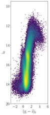 |
Fig. B.2. CMD for all the ϖ-background stars in Baade’s Window with μℓ* < −5 mas yr−1. |
Appendix C: Age estimate for a field at higher Galactic latitudes
The top panel in Fig. C.1 shows the cleaned CMDs for the bulge field at (ℓ,b) = (0° , − 6° ). The field is chosen on the bulge minor axis, further away from the plane with the respect to Baade’s window. We assume a distance of 8 kpc to convert observed magnitudes into absolute ones, and we overplot MIST isochrones with [Fe/H]= − 0.1 and [α/Fe]= + 0.1 (Johnson et al. 2022). In this field, we can clearly rule out the presence of stars younger than 2 Gyr, and exclude a significant population of young stars with ages ≲5 Gyr, which would have been apparent with a brighter MSTO. This is consistent with the results presented for Baade’s window in Section 5.4.
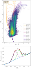 |
Fig. C.1. Top: Clean bulge de-reddened CMD for sources within 1° from (ℓ,b) = (0° , − 6° ), with overplotted a selection of MIST isochrones with [Fe/H]= − 0.1 and [α/Fe]= + 0.1. Bottom: distribution absolute magnitudes for sources with (g − i)0 ≥ 0.8 (dash-dotted line in top panel), with Gaussian fits to the double RC (purple and green curve) and to the RGB bump (blue curve). |
Following the same approach described in Section 5.4, in the bottom panel of Fig. C.1 we show the luminosity function for stars with (g − i)0 ≥ 0.8. In this field, we clearly observe the double RC, which is caused by the X-shaped nature of the bulge, and the distance distribution of sources along this line of sight (e.g. Nataf et al. 2010; McWilliam & Zoccali 2010; Gonzalez et al. 2015; Lim et al. 2021). For the bright (faint) RC, we fitted a mean magnitude Mi0 = 0.48 (Mi0 = 0.92) and a standard deviation of 0.23 (0.20). The RGB bump is instead observed at Mi0 = 1.49, with a standard deviation of 0.20. For this field, we try to fit 4 Gaussian distributions to identify both components of the RGB bump, but we are not able due to its overlap with the RCs.
The application of the method introduced in Section 5.4, using the distance between the RGB bump and the RC as a proxy for the age of the stars in the field, requires a precise (and unambiguous) detection of the two features in the observed CMD. A direct application of equation (12) to the field at (ℓ,b) = (0° , − 6° ) would result in an unphysical age of ∼21 Gyr, because of the large difference of ∼1 mag between the RGB bump and the RC (see Fig. 17). This mismatch could be explained by the overlap between the faint RC and the bright component of the RGB bump, which is less populated compared to the RC (e.g. Renzini & Fusi Pecci 1988; Nataf et al. 2011). To summarize, the presence of stars with different metallicities and different distances along the line of sight complicates the picture, and a detailed modelling of the complex three-dimensional morphology of the Galactic bulge is required before this method can be applied to all the bulge fields discussed in this work.
All Tables
All Figures
|
Fig. 1. Logarithmic density, in Galactic coordinates, of all the sources from the BDBS/Gaia EDR3 matched catalogue. The colour is proportional to the number of stars in each bin. The bins have sizes of 2.26′×2.26′. The dashed box marks the region where we can use the extinction map derived by Simion et al. (2017). The red circle shows the location of the field centred on Baade’s window with a radius of 1°, analysed in Sect. 3. The black squares show the bulge fields examined in Sect. 4, each covering an area of 1 deg2. The blue-filled circles correspond to the known clusters in the field, taken from the catalogue of Harris (1996, 2010 edition). |
| In the text | |
|
Fig. 2. Uncertainties in Gaia EDR3 proper motions in right ascension as a function of G magnitude for all the sources in the BDBS/Gaia EDR3 matched catalogue. The median value is shown with a solid black line, and the grey shaded area corresponds to the 1-sigma confidence interval, computed using the 16th and 84th percentiles of the distribution. |
| In the text | |
|
Fig. 3. Observed dereddened CMD for all the ∼1.3 × 10⁶ sources in Baade’s window, passing the quality cuts on the Gaia EDR3 astrometry and BDBS photometry. The horizontal dashed line marks the cut at i0 = i0, max − 3σi = 16.1 which we employ at the end of Sect. 3 to remove the MSTO and compute the ratio of blue to red stars in the field. |
| In the text | |
|
Fig. 4. Astrometric cleaning procedure using Gaia parallaxes. Left: dereddened BDBS CMD for all the ϖ-foreground stars in Baade’s window, defined as the sources with (ϖ−ϖZP) > 0.2 mas and σϖ/(ϖ−ϖZP) < 0.2. Middle: BDBS CMD for the ϖ-background sources. Right: distribution of proper motions in Galactic longitude (top) and latitude (bottom) for ϖ-foreground (blue) and ϖ-background (red) stars. The vertical dashed line corresponds to the cut in μℓ* employed by Clarkson et al. (2008) to select bulge members. |
| In the text | |
|
Fig. 5. Left: de-reddened CMD for all the ϖ-background sources in Baade’s Window, cleaned from foreground contaminants using Gaia EDR3 parallaxes. Colour is proportional to the logarithm of the density of sources. Middle: same CMD, colour-coded by the mean value of the proper motion in Galactic longitude. Right: same CMD, colour-coded by the mean value of the proper motion in Galactic latitude. To compare the proper motion values to their typical uncertainty in Gaia EDR3 (see Fig. 2), we note that i0 = 17 corresponds roughly to G = 18.5. |
| In the text | |
|
Fig. 6. Distribution of proper motion in Galactic longitude as a function of colour for the ϖ-background sources in Baade’s window. The red curve is the median value of μℓ* for each bin in (g − i)0, and the width of the red band is computed using the 16th and the 84th percentiles of the distribution of proper motions in each bin. The black dashed horizontal line corresponds to the mean of the Gaussian fitted to the distribution of the bulge stars. |
| In the text | |
|
Fig. 7. Result of the GMM applied to the distribution of Galactic proper motions for ϖ-background stars in Baade’s window. The red and blue bivariate Gaussian distributions correspond to the bulge and to the μ-foreground population, respectively. The black curve is the sum of the two Gaussian distributions, and the crosses mark the position of the mean of the distributions. The parameters of the two distributions are summarized in Table 1. |
| In the text | |
|
Fig. 8. De-reddened CMD for all the ϖ-background sources in Baade’s Window, colour-coded by the probability of bulge membership according to Gaia EDR3 proper motions (Eq. (8)). |
| In the text | |
|
Fig. 9. Density plots illustrating the parallax and proper motion cleaning of the dereddend CMD for stars in Baade’s window. Left: all sources with reliable BDBS photometry and Gaia EDR3 astrometry. Middle: same as middle panel in Fig. 4, ϖ-background sources surviving the Gaia EDR3 parallax cuts. Right: subset of the ∼3.3 × 10⁵ sources with Gaia EDR3 proper motions consistent with a bulge membership, according to the GMM. The blue histograms above the CMDs represent the corresponding normalized distributions of (g − i)0 for stars brighter than i0, max − 3σi = 16.1 (shown as a horizontal dashed line in all three plots). The dashed curves correspond to the two fitted Gaussian distributions, and the black curve to their sum. The corresponding value of fB (the ratio between blue and red stars) is reported in each panel. |
| In the text | |
|
Fig. 10. Top: a selection of MIST isochrones adopting solar composition overlaid on BDBS photometry in Baade’s window, after the parallax and proper motion cleaning. The absolute magnitude in the i band Mi0 is computed assuming a fiducial distance of 8 kpc for all the stars. |
| In the text | |
|
Fig. 11. Extinction-corrected and foreground-cleaned bulge CMDs for Galactic fields with |ℓ| ≤ 9° (rows), −9° ≤b ≤ −3° (columns), with a step of 1°. Each field contains all the sources within a square of 1 deg2. Galactic longitude ℓ increases towards the left of the plot, so that the plot in the top left corresponds to (ℓ,b) = (9° , − 3° ), and the one in the bottom right to (ℓ,b) = (−9° , − 9° ), as shown by the black circles in Fig. 1. |
| In the text | |
|
Fig. 12. Same as Fig. 11, but showing only the foreground sources in each field (selected using both Gaia EDR3 parallaxes and proper motions). |
| In the text | |
|
Fig. 13. First row: maximum contamination to the bulge CMDs from stars with proper motions consistent with belonging to the foreground population. Second row: ratio of foreground to background stars. Third row: maximum of the i0 distribution (for i0 > 17). Fourth Row: ratio of blue to red stars, when only stars with i0 ≤ i0, max − 3σi are considered. All the plots are shown as a function of Galactic coordinates, for the bulge fields shown in Fig. 1. |
| In the text | |
|
Fig. 14. Kinematic transverse maps derived from the parameters of the Gaussian distribution of the bulge members fitted to Gaia EDR3 proper motions, for the same bulge fields shown in Fig. 1. From top to bottom, we show the mean proper motions in Galactic longitude and latitude, the proper motion dispersions in Galactic longitude and latitude, the dispersion ratio, and the correlation between the proper motions. |
| In the text | |
|
Fig. 15. From top to bottom, we show the mean proper motion in ℓ for blue stars, the mean proper motion in ℓ for red stars, the dispersion in proper motions in ℓ for blue stars, the dispersion in proper motions in ℓ for red stars, and the difference between the mean proper motions in ℓ for blue and red stars. All the plots are shown as a function of Galactic coordinates, for the southern bulge fields shown in Fig. 1. |
| In the text | |
|
Fig. 16. Gaussian fits to the absolute magnitude distribution for sources in Baade’s window with (g − i)0 ≥ 0.8 (dash-dotted vertical line in Fig. 10). The purple curve corresponds to the RC, while the blue one to the RGB bump. Absolute magnitudes are computed assuming a mean distance of 8 kpc for all the stars. |
| In the text | |
|
Fig. 17. Distance between the RGB bump and the RC in the i band as a function of age for MIST isochrones of different metallicities and alpha abundances. The lines are linear fits to the theoretical points. The black dot, with its uncertainties, corresponds to the value obtained in this work for stars in Baade’s Window. |
| In the text | |
|
Fig. 18. Set of MIST isochrones for [Fe/H] = 0 and [α/Fe] = 0 (top panel), and [Fe/H] = +0.3 and [α/Fe] = 0 (bottom panel). The black point corresponds to the fitted value of the RGB bump in Baade’s window, assuming a mean age for the stars of 10 Gyr, and a mean solar metallicity. |
| In the text | |
|
Fig. A.1. Number of Gaussian components in the GMM minimizing the median BIC, for the bulge fields shown in Fig. 1. |
| In the text | |
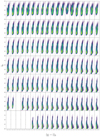 |
Fig. B.1. Same as Fig. 11, but considering only sources with μℓ* < −5 mas yr−1. |
| In the text | |
|
Fig. B.2. CMD for all the ϖ-background stars in Baade’s Window with μℓ* < −5 mas yr−1. |
| In the text | |
|
Fig. C.1. Top: Clean bulge de-reddened CMD for sources within 1° from (ℓ,b) = (0° , − 6° ), with overplotted a selection of MIST isochrones with [Fe/H]= − 0.1 and [α/Fe]= + 0.1. Bottom: distribution absolute magnitudes for sources with (g − i)0 ≥ 0.8 (dash-dotted line in top panel), with Gaussian fits to the double RC (purple and green curve) and to the RGB bump (blue curve). |
| In the text | |
Current usage metrics show cumulative count of Article Views (full-text article views including HTML views, PDF and ePub downloads, according to the available data) and Abstracts Views on Vision4Press platform.
Data correspond to usage on the plateform after 2015. The current usage metrics is available 48-96 hours after online publication and is updated daily on week days.
Initial download of the metrics may take a while.