| Issue |
A&A
Volume 664, August 2022
|
|
|---|---|---|
| Article Number | A79 | |
| Number of page(s) | 30 | |
| Section | Planets and planetary systems | |
| DOI | https://doi.org/10.1051/0004-6361/202142912 | |
| Published online | 11 August 2022 | |
K2 and Spitzer phase curves of the rocky ultra-short-period planet K2-141 b hint at a tenuous rock vapor atmosphere
1
Max-Planck-Institut für Astronomie,
Königstuhl 17,
69117
Heidelberg, Germany
e-mail: This email address is being protected from spambots. You need JavaScript enabled to view it.
2
Leiden Observatory, Leiden University,
Niels Bohrweg 2,
2333
CA Leiden, The Netherlands
3
Centre for Research in Earth and Space Sciences, York University,
4700 Keele St,
Toronto,
ON M3J 1P3
Canada
4
SRON Netherlands Institute for Space Research,
Niels Bohrweg 4,
2333
CA Leiden, The Netherlands
5
Department of Earth & Planetary Sciences, McGill University,
3450 rue University,
QC H3A 0E8
Montréal, Canada
6
Department of Physics, McGill University,
3600 rue University,
Montréal,
QC H3A 2T8
Canada
7
Atmospheric, Oceanic & Planetary Physics, Department of Physics, University of Oxford,
Oxford,
OX1 3PU,
UK
8
Université de Montréal, Institut de Recherche sur les Exoplanètes,
1375 Ave.Thérèse-Lavoie-Roux,
Montréal,
QC H2V 0B3
Canada
9
Department of Physics, Oxford University,
Parks Rd,
Oxford,
OX1 3PJ
UK
10
Department of Physics, University of Warwick,
Coventry,
CV4 7AL
UK
11
Eureka Scientific Inc,
Oakland,
CA 94602
USA
12
Dipartimento di Fisica e Astronomia "Galileo Galilei", Università degli Studi di Padova,
Vicolo dell'Osservatorio 3,
35122
Padova, Italy
13
INAF - Osservatorio Astronomico di Padova,
Vicolo dell'Osservatorio 5,
35122
Padova, Italy
14
Johns Hopkins APL,
11100 Johns Hopkins Rd,
MD 20723
Laurel, USA
Received:
14
December
2021
Accepted:
1
March
2022
Abstract
K2-141 b is a transiting, small (1.5 R⊕) ultra-short-period (USP) planet discovered by the Kepler space telescope orbiting a K-dwarf host star every 6.7 h. The planet's high surface temperature of more than 2000 K makes it an excellent target for thermal emission observations. Here we present 65 h of continuous photometric observations of K2-141 b collected with Spitzer's Infrared Array Camera (IRAC) Channel 2 at 4.5 μm spanning ten full orbits of the planet. We measured an infrared eclipse depth of  ppm and a peak to trough amplitude variation of
  ppm. The best fit model to the Spitzer data shows no significant thermal hotspot offset, in contrast to the previously observed offset for the well-studied USP planet 55 Cnc e. We also jointly analyzed the new Spitzer observations with the photometry collected by Kepler during two separate K2 campaigns. We modeled the planetary emission with a range of toy models that include a reflective and a thermal contribution. With a two-temperature model, we measured a dayside temperature of
  K and a night-side temperature that is consistent with zero (Tp,n < 1712 K at 2σ). Models with a steep dayside temperature gradient provide a better fit to the data than a uniform dayside temperature (ΔBIC = 22.2). We also found evidence for a nonzero geometric albedo
  . We also compared the data to a physically motivated, pseudo-2D rock vapor model and a 1D turbulent boundary layer model. Both models fit the data well. Notably, we found that the optical eclipse depth can be explained by thermal emission from a hot inversion layer, rather than reflected light. A thermal inversion may also be responsible for the deep optical eclipse observed for another USP, Kepler-10 b. Finally, we significantly improved the ephemerides for K2-141 b and c, which will facilitate further follow-up observations of this interesting system with state-of-the-art observatories such as James Webb Space Telescope.
Key words: planets and satellites: atmospheres / planets and satellites: individual: K2-141 b / techniques: photometric
© S. Zieba et al. 2022
 Open Access article, published by EDP Sciences, under the terms of the Creative Commons Attribution License (https://creativecommons.org/licenses/by/4.0), which permits unrestricted use, distribution, and reproduction in any medium, provided the original work is properly cited.
Open Access funding provided by Max Planck Society.
1 Introduction
The field of exoplanetary science started off with the surprising discovery of planets with short orbital periods. The formation of these planets has been well studied and still remains a puzzle to this day (see e.g., Dawson & Johnson 2018). Ultra-short-period (USP) planets are an extreme subgroup of this population with orbital periods shorter than one day (for a review of USPs see e.g., Winn et al. 2018). The majority of these planets have been found to be smaller than 2R⊕ (Sanchis-Ojeda et al. 2014; Lundkvist et al. 2016).
One early theory was that these small USP planets could be remnant bare cores of hot Jupiters that lost their envelopes due to photoevaporation, Roche overflow, or other processes (Jackson et al. 2013). It was however shown that the well-known planet–metallicity correlation (Fischer & Valenti 2005) is not observed for USP planets (Winn et al. 2017). USP planets are therefore probably not evaporated hot Jupiters, but there is still no consensus about whether they are born rocky or whether they once had amodest hydrogen envelope (Van Eylen et al. 2018; Lopez 2017). As USPs and sub-Neptunes (planets between 2 R⊕ and 4 R⊕) generally orbit stars with similar metallicities, sub-Neptunes might be possible progenitors. Most USPs have Earth-like densities (Dai et al. 2019), but a few (55 Cnce; Crida et al. 2018b,a) (WASP-47e; Vanderburg et al. 2017) have lower densities consistent with a low iron fraction or a small volatile envelope. Direct observations of the planet’s atmospheres are needed to distinguish between these scenarios.
55 Cnce (Fischer et al. 2008; Dawson & Fabrycky 2010; Winn et al. 2011; Demory et al. 2011), is one of the best-studied small USP planets and shows evidence for a thick atmosphere (Demory et al. 2016a; Angelo & Hu 2017). It is one of the very few small planets (<2 R⊕) for which thermal emission was observed in the infrared (others include LHS 3844 b by Kreidberg et al. (2019) and K2-141 b in this work). Most other USP planets have been observed in the visible light with missions such as CoRoT (Auvergne et al. 2009), Kepler (Borucki et al. 2010), K2 (Howell et al. 2014), or more recently TESS (Ricker et al. 2014). Numerous observations of 55Cnce with Spitzer have shown some surprising results: a large hotspot offset, where the hottest region of the planet is significantly offset from the substellar point (Demory et al. 2016a). This phase curve offset could be explained by a thick atmosphere with a super-rotating jet that advects energy away from the substellar point (Kite et al. 2016; Hammond & Pierrehumbert 2017; Angelo & Hu 2017). Demory et al. (2016b) furthermore reported varying observed dayside temperatures for 55 Cnc e ranging from 1300 K to 2800 K. The authors propose that these observed changes were possibly caused by volcanic activity, leading to plumes which increase the opacity in the Spitzer bandpass. Tamburo et al. (2018) reanalyzed the Spitzer observations and conclude that the changing eclipse depths were best modeled by a year-to-year variability model. They also suggest that the dayside of the planet is intermittently covered with reflective grains obscuring the hot surface, possibly originating from volcanic activity or cloud variability. Despite the numerous observations of 55Cnce, its composition and structure still remains puzzling. Dorn et al. (2019) suggest that the low observed density of 55Cnce (6.4 ± 0.3 g/cm3) might be explained by the planet being a part of a new class of Super-Earths which formed from high-temperature condensates. Planets similar to this would have no core and have enhancements in Ca, Al rich minerals leading to a lower overall bulk density compared to an Earth-like (30% Fe and 70% MgSiO3) or a pure MgSiO3 composition.
Recent observations of 55 Cnc e with TESS also showed a tentative deep optical eclipse, which could be caused by a nonzero albedo if confirmed (Kipping & Jansen 2020). Other observations of 55 Cnc e in the optical by the Microvariability and Oscillations in Stars (MOST) space telescope (Winn et al. 2011) showed a quasi-sinusoidal modulation of flux with the same period as the planet. The amplitude of the signal was, however, too large to be reflected light or thermal emission alone and its origin remained unclear in that study. Additional MOST observations spanning several weeks between 2011 and 2015 by Sulis et al. (2019) confirmed this optical modulation. The amplitude and phase of the signal were variable which the authors suggested might be due to some star-planet interaction or the presence of a transiting circumstellar dust torus. They also did not detect the secondary eclipse of the planet which led to an upper value for the geometric albedo of 0.47 (2σ). Furthermore, recently Morris et al. (2021) presented CHEOPS observations of the planet showing a large phase variation but they do not detect a significant secondary eclipse of the planet. The authors suggest that the origin of the signal might be from circumstellar or circumplanetary material modulating the flux of the system. This is just another example of the challenges to determine the nature of 55 Cnce.
Another surprising discovery came with Kepler-10b (Batalha et al. 2011), the first rocky planet detected by the Kepler mission. The planet showed a deep secondary eclipse that suggested an unusually high reflectivity in the Kepler bandpass (Batalha et al. 2011; Rouan et al. 2011; Sheets & Deming 2014). A high albedo for planets that are highly irradiated by their stars could be explained by the creation of calcium- and aluminumrich surfaces on their dayside (Léger et al. 2011; Rouan et al. 2011; Kite et al. 2016; Modirrousta-Galian et al. 2021). A subset of planets detected by Kepler showed comparably high albedos in the optical wavelengths (Demory 2014). Most notably, both Kepler-10b and Kepler-78b (Sanchis-Ojeda et al. 2013) have albedos of 0.4–0.6 (Sheets & Deming 2014). Hu et al. (2015) reanalyzed the Kepler data of Kepler-10b and did not detect any phase curve offset. They found that any model with a Bond albedo greater than 0.8 fits the visible phase curve well regardless of whether asymmetric reflection exists.
Due to the high irradiation small USP planets receive from their host stars, they are more susceptible to atmospheric loss (Lopez 2017). LHS 3844b (Vanderspek et al. 2019), an USP planet orbiting an M-type star, was clearly shown to lack a thick atmosphere using observations by the Spitzer Space Telescope and is therefore likely a bare rock (Kreidberg et al. 2019). The 100h continuous phase curve of the planet showed no hotspot offset ruling out the possibility of a thick atmosphere, and any less-massive atmospheres would be unstable to erosion by stellar wind. Some planets might however retain an atmosphere by the evaporation of surface lava oceans leading to a silicate rich atmosphere (Schaefer & Fegley 2010; Miguel et al. 2011) or might have other thick, high mean-molecular-weight atmospheres (Demory et al. 2016a).
Here we present Spitzer observations of the USP K2-141 b (EPIC 246393474 b). The planet was discovered in 2018 by Malavolta et al. (2018) and independently by Barragán et al. (2018) using observations of the Kepler telescope during its “second light” mission, K2 (Howell et al. 2014). The planet has a radius of Rp = 1.51 ± 0.05 R⊕ and orbits its K-dwarf host star every 0.28 days (6.7 hours). Observations of the star by the high-precision spectrograph HARPS-N measured a mass for the planet (Mp = 5.08 ± 0.41 M⊕). With a density of ρ = (8.2 ± 1.1) g/cm3, K2-141b is mostly consistent with an Earth-like iron-silicate composition. The radial velocity observations furthermore confirmed another companion K2-141c, which is in radius and upper mass more likely to be a Neptunelike planet than a rocky planet or a HJ, orbiting further out with an orbital period of 7.7 days.
The Kepler observations also revealed the optical phase curve and secondary eclipse with a depth of 23 ± 4 ppm. The equilibrium temperatures of K2-141 b, Kepler-10b and 55 Cnce are 2150 K, 2170 K and 1950 K in case of full atmospheric heat redistribution and 2745 K, 2775 K and 2490 K for instant reradiation, respectively1. K2-141 b is therefore a perfect target to compare to other well studied USPs (see also Table 1). Its host star is also bright enough (V = 11.5 mag, K = 8.4 mag) to conduct follow-up observations of the planet’s emission in the infrared as previously done with 55 Cnce (V = 6.0mag, K = 4.0mag) (Demory et al. 2016a,b). K2-141 b and 55 Cnc e are therefore the only two currently known small USPs which are accessible in both the optical and infrared which invites comparison between the two planets. We note, however, the difference in densities for the planets: while K2-141 b’s density is consistent with an Earth-like composition (30% Fe), is 55 Cnc e inconsistent with an Earth-like composition at over 4σ2.
Recently, Nguyen et al. (2020) modeled the atmosphere of K2-141 b assuming the planet has a thin rock vapor atmosphere which arises from the evaporation of the surface on the dayside. This leads to a flow that is maintained by the pressure gradient between the nightside and dayside on the planet. This flow is however not able to transport enough heat to the nightside to create a considerable thermal hotspot offset nor to heat the nightside. Previous studies of transit spectroscopy of lava planets focused on more volatile species such as Na or K (Castan & Menou 2011; Kite et al. 2016). Nguyen et al. (2020) compared different atmospheric compositions expected for a rock vapor atmosphere (Na, SiO and SiO2) and found that an SiO2 atmosphere may be easier to observe due to the extreme geometry of this system. Nguyen et al. (2020) also noted that due to the proximity of K2-141 b to its host star (a/R* = 2.292), the night side (the area of the planet which never receives any incident flux) is only about a third of the planet, rather than a hemisphere. The terminator for K2-141b is located approximately 115° from the substellar point, leading to a hemisphere-integrated night side temperature of approximately 400 K for the planet3. Therefore, the regions probed during a transit range from ~65° to ~115° from the substellar point. If the planet is further away from the star the region probed during a transit is approximately 90° from the substellar point. This effect is so small, however, that the flux emitted from the night side would not be detectable within the measurement precision of our data. We therefore adopt a night hemisphere in this paper.
The paper is structured as follows: Sect. 2 describes the data reduction of the K2 and Spitzer observations used in this paper. Section 3 discusses the different models which were fit to the K2 and Spitzer data to extract information on the reflective and thermal emission coming from the planet. Section 4 compares the observations to two different atmospheric models: a pseudo-2D rock vapor model and a 1D turbulent boundary layer model, the latter being recently published in Nguyen et al. (2020) and further improved in Nguyen et al. (2022). In Sect. 5 we discuss our findings and summarize our conclusions in Sect. 6.
Selection of USPs and their properties.
2 Observations and Data Reduction
2.1 Spitzer Photometry
We observed the K2-141 system with the Spitzer InfraRed Array Camera (IRAC; Fazio et al. 2004) for about 65 h between October 09 and October 11, 2018 (Program 14135, Kreidberg et al. 2018). We used Channel 2 on IRAC (equivalent to a photometric bandpass of 4–5 µm) with a two-second exposure time. The observations began with a 30-min burn-in to allow for the telescope to thermally settle. Following this procedure, we placed the target on the “sweet spot”, a pixel on the detector which is known to have a minimal intra-pixel sensitivity variation.
We split the observations into six sequential datasets (AORs, Astronomical Observation Requests) which we downloaded from the Spitzer Heritage Archive4 (see Table 2 for the start and end time of each individual AOR). We reduced the Basic Calibrated Data (BCD, provided by the Spitzer Science Center) with the Photometry for Orbits, Eclipses, and Transits (POET) pipeline (which is available open-source on GitHub5) developed by Stevenson et al. (2012) and Cubillos et al. (2013). It performs centroiding on each frame by fitting a 2D Gaussian profile to the stellar image (Lust et al. 2014) in each Spitzer exposure after upsampling by a factor of five in each spatial direction (Harrington et al. 2007). The target remains centered near the sweet spot for the entire AOR in each observation, with the majority of the exposures being well within of 0.1 pixels from the sweet spot (see plots in Appendix C.2). POET then identifies and flags bad pixels using an iterative sigma-clipping procedure along the time axis and then sums the flux in each fixed aperture. We have chosen a grid of apertures with radii ranging from two to four pixels in 0.25 pixel steps for every AOR and used the aperture which minimizes the residual noise in each of the extracted light curves (a list of the apertures can be found in Table 3). For the median background flux estimation, we used an annulus with an inner radius of 7 pixels and outer radius of 15 pixels.
The dominant systematics for the 4.5 µm Spitzer channel are intrapixel sensitivity variations (Charbonneau et al. 2005; May & Stevenson 2020). We therefore fit for them by using the BiLinearlyInterpolated Subpixel Sensitivity (BLISS) map technique introduced by Stevenson et al. (2012) (see plots in Appendix C.3 to see the determined intrapixel sensitivity variations across the detector). We determined the pixel bin size used for the map for every AOR and listed it in Table 3.
We visually inspected the data and removed three short segments of data (two in AOR3 and one in AOR5) making up approximately 5% of the observations that showed strong correlated noise in the residuals. After visually inspecting the individual frames during the discarded segment in AOR5 it was able to attribute this event to a strong cosmic ray hit on the detector (see Fig. C.2). The other segment in AOR3 showed no noticeable trends in PRF width or other parameters (see Fig. C.1). Similar outliers were also observed in previous observations using Spitzer’s IRAC Channel 2 (e.g., Kreidberg et al. 2019; Challener et al. 2021). For the majority of the observations, the target fell well within 0.5 pixels around the sweet spot. We removed an additional 0.3% of exposures in the third AOR because these exposures had a centroid position shifted by a whole pixel in the x-dimension.
Observations with Kepler and Spitzer used in this work.
Parameters used for the data reduction of every Spitzer AOR determined by minimizing the Bayesian Information Criterion (BIC).
2.2 K2 Photometry
2.2.1 Campaign 12
K2’s campaign 12 (C12) was carried out by the Kepler space telescope from December 15, 2016, to March 04, 2017. The photometric data were taken in the long cadence sampling rate (~30 min) over a timespan of about 79 days. The data extraction and reduction is described in Malavolta et al. (2018) and was reused for this analysis.
2.2.2 Campaign 19
K2’s campaign 19 (C19) was carried out from August 30, 2018 to September 26, 2018 and marked the last observations taken by the Kepler space telescope before running out of fuel. C19’s field-of-view overlapped with C12 leading to a reobservation of K2-1416. The fuel shortage on the spacecraft, however, led to a shorter campaign. These last data taken by Kepler span only about a month and suffer from erratic pointing at the beginning and end of the campaign. We removed approximately 54% of the data leaving us with approximately 7 days of observations with a photometric precision comparable to other K2 Campaigns. Approximately 8.5 days at the beginning of the observations were removed because the boresight of the telescope was off-nominal leading to K2-141 being completely out of the pixel stamp. We also removed the final 11 days of the observations where the boresight and roll of Kepler fluctuated erratically7. In contrast to C12, the observations of K2-141 in C19 were taken in the short cadence mode with a sampling rate of about one minute. Due to this higher temporal resolution, there is no need to oversample the C19 data.
The photometry was accessed with the python package lightkurve (Lightkurve Collaboration 2018), which retrieves the data from the MAST archive8. We downloaded the Simple Aperture Photometry (SAP) data and removed every measurement with a nonzero “quality” flag, which indicates events like thruster firings or cosmic ray hits.
We used the self-flat-fielding (SFF) procedure described in Vanderburg & Johnson (2014) and Vanderburg et al. (2016), which is implemented in lightkurve, to correct for the systematic flux variations of the K2 data caused by thruster firings every six hours. In addition to the six hour back and forth movement throughout the K2 mission, there was also transverse spacecraft drift on timescales longer than 10 days (Vanderburg et al. 2016). We therefore subdivided the 8 days of data into two “windows” and performed the SFF independently in each of them. To remove outliers, we fit a cubic spline to the data and performed an iterative sigma clipping with respect to the median to mask outliers at 5σ below and 3σ above the light curve, which removed 0.3% of the remaining C19 data. We then normalized the data by dividing by the median of the flux.
To remove the stellar variability (Prot ~ 14 days, Malavolta et al. 2018), we fit a linear function of time to the out-of-transit data for each orbit (eclipse to eclipse) while masking the transits following Sanchis-Ojeda et al. (2013). For each orbit, the linear function was then subtracted from the data and unity was added. The observations contain 25 full phases (eclipse to eclipse) of the planet around the star. The C19 observations also contain one transit of K2-141 c which we removed from our analysis, but use in Appendix A to improve the ephemeris of K2-141 c.
3 Light Curve Fits
We considered fits to the Spitzer data alone (see Sect. 3.1), and to the joint Spitzer and Kepler dataset (see Sect. 3.3). For every model described in the following section we performed a differential evolution Markov chain Monte Carlo (MCMC) (Ter Braak 2006) analysis to estimate parameter uncertainties. We rescaled the uncertainties for every data point by a constant factor so that the reduced chi-squared is unity and we get realistic uncertainties for the fit parameters. The chi-squared values before rescaling based on the final best fitting model in our analysis can be found in Table B.1. We ran the MCMC until all free parameters of four initialized chains converged to within 1% of unity according to the Gelman-Rubin statistic (Gelman & Rubin 1992). Each chain consisted out of 10 000 steps and we discarded the first 50% of the MCMCs as burn-in. This leaves us with a total of 20 000 steps for each run. We include plots of the resulting posterior distributions in Appendices C.5 to C.10.
The transit model implemented in BATMAN (Kreidberg 2015) which was used in every fit, consists of the time of central transit t0, the radius of planet in units of stellar radii Rp/R*, the orbital period P, semi-major axis in units of stellar radii a/R* and the cosine of the inclination cos i. We fixed the eccentricity ecc and the argument of periastron ω to zero. This is justified due to the very short circularization time scale of these USPs. Following equation 3 from Adams & Laughlin (2006), the circularization time scale for K2-141 b is only about τcirc = 3.1 Myr assuming a tidal quality factor of QP = 106. We used the ExoCTK limb darkening calculator (Batalha et al. 2017) and the stellar parameters given in Malavolta et al. (2018) to determine and fix the linear and quadratic limb-darkening coefficients u1 and u2. They are u1 = 0.105 and u2 = 0.119 in the Spitzer IRAC Channel 2 bandpass and u1 = 0.666 and u2 = 0.062 in the Kepler bandpass.
3.1 Spitzer Only Fit
We model the full Spitzer light curve, F(x, y, X, Y, t), as:
 (1)
(1)
where Fs is the constant out-of-transit flux (i.e., the stellar flux), R(t) is the ramp model, M(x, y) is the BLISS map with (x, y) describing the position of the star on the detector, T(t) is the Mandel & Agol (2002) transit model implemented in BATMAN (Kreidberg 2015), E(t) is the eclipse model implemented in BATMAN and P(t) the phase variation in SPIDERMAN (Louden & Kreidberg 2018) or POET Cubillos et al. (2013) (depending on which specific model was used). G(X, Y) is a term fitting for variations in the pixel response function (PRF) using a 2D cubic (i.e., PRF-FWHM detrending, see e.g., Lanotte et al. 2014; Mendonça et al. 2018; May & Stevenson 2020) and has the following form:
 (2)
(2)
where X1 (Y1), X2 (Y2), and X3 (Y3) are the linear, quadratic and cubic coefficients in the X (Y) dimension, respectively, and sx and sy the Gaussian widths of the pixel response function in the X (Y) dimension, respectively. The optimal resolution for BLISS mapping, the ramp model R(t) (either a constant or linear ramp) and the order of the PRF fit G(X, Y) were independently determined by minimizing the Bayesian Information Criterion (BIC) for every AOR and are listed in Table 3.
Equation (1) describes the general model which was fit to the Spitzer data. For this model, the orbital period P was fixed to the literature value reported in Malavolta et al. (2018). For parameters which are more precisely determined by the K2 data, namely t0, Rp/R* a/R* and cos i, we used Gaussian priors in our analysis based on the literature values.
We fit three different phase variation models P(t) to the Spitzer data. First, a sinusoid with amplitude A multiplied by an eclipse model with eclipse depth fp/f* and including a phase offset ϕ of the hotspot. Second, same as above but without a phase offset. Third, a two temperature model for the planet with a constant temperature on the dayside, Tp,d, and on the nightside, Tp,n. A list of the free parameters for every model is listed in the Appendix (see Table B.2).
A commonly approach for model selection in the exo-planet literature is using the Bayesian Information Criterion (BIC, Schwarz 1978; Kass & Raftery 1995; Liddle 2007). It approximates the evidence E and has the following form:
 (3)
(3)
where ℒmax is the maximum likelihood of the model, k the number of free parameters of the model and N the number of data points. The BIC therefore penalizes models with more free parameters and the best-fitting model is the one with the lowest BIC (i.e., the largest evidence). We compare models by calculating ΔBIC:
 (4)
(4)
with BICmin being the smallest BIC of the set of models being compared. By taking the difference of BIQ and BICmin, several constants cancel out and we are left with: BIC = χ2 + k ln N, which now includes the χ2 value of the model. When comparing two models, Kass & Raftery (1995) lists a ΔBIC > 3.2, ΔBIC > 10, ΔBIC > 100 as being a substantial, strong, decisive evidence for the model with the lower BIC, respectively.
The symmetric sinusoidal model with no hotspot offset is statistically substantially preferred with ΔBIC > 8.8 (see Table 4) compared to a sinusoid with an offset. We therefore find the data are consistent with the peak brightness occurring at the substellar point, in contrast to the prominent USP planet 55 Cnce which has an eastward offset of 41° ± 12° (Demory et al. 2016a). When we include an offset as a free parameter, we obtain  (the negative sign denotes an offset westward from the substellar point). We measure an eclipse depth in the Spitzer bandpass
  ppm and an amplitude variation
  ppm. We note that the reflected light contribution at 4.5 µm has not been subtracted from the brightness temperature computation. Table 4 lists all best fit parameters and their uncertainties. A comparison of the BIC between the models showed that the sinusoidal model with no hotspot offset fits best to the Spitzer data. We show the best fitting model with the Spitzer observations in Fig. 1.
3.2 Goodness of Spitzer Only Fit
We tested for the presence of red noise by comparing the root-mean-square (rms) of the binned residuals of the light curve with the predictions from white noise. If the data are uncor-related (white) in time, the rms of the residuals is expected to decrease with  , where N is the number of data in a bin. A bin size of one, therefore, denotes no binning at all. We combined all six datasets and subtracted the best fitting model. Figure 2 shows that the residuals of the Spitzer data agree well with the expectations from uncorrelated noise. The same figures for each individual Spitzer AOR can be found in Appendix C.4.
 |
Fig. 1 Phase curve of K2-141 b after phase folding the complete Spitzer observations. The eclipse is at phase = 0.5. The best fitting model shown in red describes the observed thermal emission from the planet as a sinusoidal function. Each bin in black (gray) consists out of 7200 (1800) Spitzer 2-s exposures. The pairs plot for this model can be found in the Appendix C.5. |
All models fit to the Spitzer data alone.
3.3 Joint Spitzerand Kepler Fit
The phase variation P(t) for the joint fit consists of a thermal Ptherm(t) and a reflective Prefl(t) contribution, with P(t) = Ptherm(t) + Prefl(t). For the reflected light component Prefl(t), we assumed a uniform Lambertian reflector (Seager 2010):
 (5)
(5)
where Ag is the geometric albedo and the orbital phase z(t) is described by:
 (6)
(6)
We fit three thermal emission models to the combined Spitzer and K2 dataset. First, a toy model described in Kreidberg & Loeb (2016) with the planet’s heat redistribution F as a free parameter. Second, same as above but with the redistribution fixed to zero leading to a nightside temperature of 0 K. Third, a two temperature model with a constant temperature on the dayside, Tp,d, and on the nightside, Tp,n. A list of the free parameters for every model is listed in the Appendix (see Table B.3). The toy heat redistribution model described in Kreidberg & Loeb (2016) expresses the temperature of the planet T(z) as a function of the zenith angle z using the following form:
 (7)
(7)
where σ is the Stefan-Boltzmann constant,  the insolation, AB the Bond albedo, z the zenith angle and 0 < F < 0.5 the heat redistribution parameter. For F = 0 no heat is being distributed and the nightside has a temperature of 0K. If F = 0.5, half of the energy received by the dayside is being transported to the nightside and the whole planet is isothermal.
With the full Spitzer and Kepler dataset, we now also fit for the orbital period P. We use Gaussian priors for T* and a/R* based on values reported in Malavolta et al. (2018): The prior for the stellar temperature is T* = (4599 ± 79) K and for semi-major axis in units of the stellar radius we use a/R* = 2.36 ± 0.06, which we derive from the stellar density ρ* = (2.244 ± 0.161)ρo following a/R* ∝ (ρ*P2)1/3.
The K2 data in Campaign 12 was collected in the long cadence mode with a sampling rate of approximately 30 min. We oversample the data by a factor of 11 as in Malavolta et al. (2018) to account for the long exposure time. The data from Campaign 19 has a shorter sampling rate of about a minute and we therefore do not oversample this data set.
The insolation parameter S for the toy model was calculated at every step in a self-consistent way, assuming  . We fit for the stellar temperature in the toy model, to take into account its uncertainty in the calculation of the insolation. In every step of the MCMC, we calculate a Kurucz model (Kurucz 1993) for the host star using the priors on the stellar temperature and stellar properties from Malavolta et al. (2018).
We tested using separate geometric albedos for the Kepler and the Spitzer dataset (Ag, K2 and Ag, Spitzer), but obtained a uniform posterior distribution for Ag, Spitzer, indicating that the Spitzer data are not able to constrain the albedo at 4.5 µm (where thermal emission dominates). We therefore used a wavelength-independent geometric albedo Ag in all subsequent fits.
The toy model includes the Bond albedo as a parameter to regulate the radiation balance of the planet. Since we assume Lambertian reflection in our analysis, the Bond albedo AB and the geometric albedo Ag are related by: AB = 3/2 Ag. While Lambertian reflectance is not an accurate model for the rocky bodies in the Solar System (Mayorga et al. 2016), this simplifying assumption is appropriate given the precision of our data and the unknown surface properties of K2-141 b. Table 5 lists all best fit parameters and their uncertainties for the joint fits and Table 6 contains some derived parameters for the best fitting model.
 |
Fig. 2 Allan deviation plot of the Spitzer data: root-mean-square (rms) of the fit residuals of the Spitzer data using the sinusoidal model without a hotspot offset (black curve) as a function of the number of data points per bin. A bin size of one depicts no binning at all. The red line shows the expected rms for Gaussian noise following the inverse square root law. |
All models fit to the joint Spitzer and K2 dataset.
3.4 Goodness of Joint Spitzerand Kepler Fit
As in Sect. 3.2 we took the observations and subtracted the best fitting model to compare the rms of the fit residuals with the expected rms for Gaussian noise. The Spitzer data agrees again well with the expectations from uncorrelated noise and looks very similar to Fig. 2. Figure 3 shows the Allan deviation plots for the two K2 Campaigns.
3.5 Improved Ephemerides
Having a precise ephemeris is crucial to schedule follow-up observations of a planet. K2-141 b is an exciting target to be observed with observatories such as JWST. In fact, Cycle 1 of JWST includes two programs to observe the planet (Dang et al. 2021; Espinoza et al. 2021). We improved the orbital period P and the transit time t0 significantly in our joint analysis using the three different datasets: the long cadence K2 C12 observations used in the discovery papers (Malavolta et al. 2018; Barragán et al. 2018), new short cadence observations during Campaign 19 of K2 and new Spitzer observations. The updated parameters for P and t0 are listed in Table 7. They are based on our joint fit using the toy model (Kreidberg & Loeb 2016) with the heat redistribution F set to zero as the resulting fit agrees best with our data. With the additional data, the 3cr uncertainty on the predicted transit time in 2024 decreases from about an hour to just 2.7 min. We also used the one transit of K2-141 c observed in K2 C19 (see Fig. 4) to improve the ephemeris of the planet. Future observers can use the updated P and t0 of K2-141 c to avoid scheduling conflicts with planet b. The analysis for K2-141 c can be found in Appendix A.
 |
Fig. 3 Allan deviation plot for K2 C12 in the left panel and K2 C19 in the right panel. |
Updated ephemeris for K2-141 b and the 3tr uncertainty on the predicted transit time in 2022 and 2024.
3.6 Results
We performed three different fits for the Spitzer data and for the joint dataset. We measured the eclipse depth in the Spitzer bandpass  ppm and an amplitude variation (peak to trough)
  ppm. The best fit is a two temperature model for the planet without a hotspot offset ϕ. When we, however, let ϕ vary, we find a value of
  , which is at a 3.9cr level strongly inconsistent with the value obtained for 55 Cnc e of 41° ± 12° (Demory et al. 2016a). For the joint analysis (Spitzer observations and the two K2 Campaigns) we find that a toy heat redistribution model from Kreidberg & Loeb (2016) without heat redistribution is most preferred. We measure a geometric albedo of
  , a dayside temperature of
  and a nightside temperature of
  (<1712 K at 2σ). A corner plot of these three parameters used in the two-temperature model can be found in Fig. 5. We found an eclipse depth in the Kepler bandpass of
  ppm which is consistent with the value reported in the discovery paper (23 ± 4 ppm, Malavolta et al. 2018). We therefore robustly detect emission coming from the dayside of K2-141b in the optical light. As a comparison, 55Cnce’s secondary eclipse detection was only seen in the TESS observations at a significance of 3σ (Kipping & Jansen 2020). We show the best fitting model to the joint data set with the Kepler observations in Fig. 6.
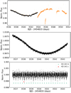 |
Fig. 4 K2 Campaign 19 data of K2-141. Upper panel: the full K2 Campaign 19 observations. We removed outliers and data suffering from decreased photometric precision due to Kepler running out of fuel (marked in orange). Middle panel: K2 C19 data with instrumental systematics removed using the SFF algorithm. Lower panel: the K2 C19 observations after removal of the stellar variability. The 25 transits by K2-141 b have been marked in green. An additional transit by K2-141 c is denoted in red. |
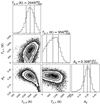 |
Fig. 5 Corner plot of the best fitting model to the joint K2 and Spitzer dataset for the dayside temperature Tp,d, the nightside temperature Tp,n and the geometric albedo Ag. |
 |
Fig. 6 Phase curve of K2-141 b as seen by Kepler during Campaign 12 and 19. Upper panel: the solid black line shows the phase curve based on the values in our best fit model (toy model without heat redistribution for the thermal emission and a uniform Lambertian reflector for the reflected light contribution). The dark orange and light orange areas around the best fitting model are the 1σ and 3σ uncertainties, respectively. We binned the Campaign 19 data that was collected in short cadence mode (~1 min) into bins of 29.4 min to have the same temporal resolution as the Campaign 12 data. We then phase folded the Kepler observations and binned the data for clarity. Each bin in black (gray) consists out of 180 (45) Kepler exposures. Lower panel: the residuals of the Kepler observations to the best fitting model. |
4 Atmospheric Constraints
In addition to the toy models presented in Sect. 3, here we compare the data to physically motivated models. K2-141b is expected to have a molten surface with a thin rock vapor atmosphere. To model the atmosphere, we used two different approaches: (1) apseudo 2-D model that includes radiative transfer for plausible chemical species, and (2) ID turbulent boundary layer model that includes mass transfer between the planet’s surface and the atmosphere.
4.1 Pseudo-2D Rock Vapor Model
We calculated pseudo-2D models for the atmosphere by dividing the planet into concentric rings in 10 degree radial increments starting at the substellar point and finishing at a zenith angle of 80° (for angles >80° the outgassed atmosphere becomes too tenuous resulting in numerical instabilities).
This modeling approach is accurate in the limit that each column of atmosphere equilibrates locally with the magma ocean, without any influence of heat or mass transport from neighboring columns. For each increment, we calculated the outgassed chemistry and temperature-pressure structure of a gas-melt equilibrium atmosphere. Our outgassed elemental budget and atmospheric pressure are determined by the results of the melt-gas equilibrium code MAGMA (Fegley & Cameron 1987; Schaefer & Fegley 2004). This is done for a volatile-free komatiite9 composition with no fractional vaporization (removal of vapor from the atmosphere) (Schaefer & Fegley 2004; Miguel et al. 2011). The outgassed chemistry and pressure are consistently adjusted for a surface temperature computed using radiative-transfer models, which are described below. We note that possible melt compositions for exoplanets are currently not known. Our choice of komatiite is based on early Earth (Miguel et al. 2011). Different melt compositions or evaporated atmospheres may result in chemistry and thermal structure changes (Zilinskas et al. 2022).
Equilibrium gas chemistry in the atmosphere is computed using a thermochemical equilibrium model FastChem10 (Stock et al. 2018). The chemistry considered includes over 30 different species for elements: O, Na, Si, Fe, Mg, K, Ti, AI, Ca and does not include ions. We do not consider the possible temporal evolution of chemistry through disequilibrium processes such as photochemistry or atmospheric mixing.
The temperature profile of the atmosphere is modeled in a radiative-convective equilibrium using a radiative transfer code HELIOS11 (Malik et al. 2017, 2019). As absorbers we include Na and SiO, for which we use a sampling wavelength resolution of λ/Δλ = 1000 and a range of 0.06–200 µm. Na opacity is computed using Vienna Atomic Line Database (VALD3) line list (Ryabchikova et al. 2015). We use the Voigt profile approximation for all, but the 0.6 µm doublet. The doublet is instead fit using unified line-shape theory of Rossi & Pascale (1985) and Allard et al. (2007a,b). The opacity of SiO is constructed using the EBJT (Barton et al. 2013) line list for ground state transitions and the Kurucz (Kurucz 1992) line list for shortwave bands. For simplicity we assume null surface albedo and black-body stellar irradiation, which may slightly overestimate incident shortwave flux. As with chemistry, temperature profiles, including the surface temperature, are consistently adjusted depending on the outgassed material. The temperature-pressure profiles of K2-141b at different zenith angles for this model are shown in Fig. 7. All zenith angles show a thermal inversion due to short-wavelength Na absorption, with a sharp increase in temperature starting at a few millibar. The amount of heating is sensitive to the UV spectrum of the star, which is unknown; however, in general thermal inversions should be expected in rock vapor atmospheres (Zilinskas et al. 2021). Future UV characterization of K2-141 would refine the theoretical predictions of the temperature structure.
To simulate emission spectra for each radial segment we use the radiative-transfer code petitRADTRANS12 (Mollière et al. 2019) with the same wavelength resolution and opacities as for the T–P profile calculation. We sum the fluxes weighted by the area of each concentric ring to calculate the total flux from the planet. Finally, we divide the planet flux by a PHOENIX stellar spectrum (Husser et al. 2013) to determine the planet-to-star contrast.
Equilibrium gas chemistry in the atmosphere leads to a decreasing surface pressure with zenith angle. Figure 8 shows the column density as a function of zenith angle for different species expected at the temperatures of K2-141 b based on calculations in Miguel et al. (2011). We show the densities for a Bulk-Silicate-Earth composition and a komatiite composition which show similar results with Na being the most abundant in both of them.
 |
Fig. 7 T–P profile of K2-141 b based on the pseudo-2D rock vapor model as described in Sect. 4.1 at different angles from the substellar point. |
4.2 1D Turbulent Boundary Layer Model
In addition to the pseudo-2D model described above, we also computed an atmospheric circulation model following Nguyen et al. (2020) and Castan & Menou (2011). The model calculates the steady-state flow induced by constant evaporation on the dayside and condensation on the nightside. Being tidally locked, we can impose symmetry across the substellar-antistellar axis by neglecting Coriolis forces. By assuming a turbulent boundary layer (TBL), we can marginalize over the vertical dimension and further reduce the problem to ID: distance from the substellar point.
This model assumes a boundary layer that is: hydrostatically-bound and behaves like a continuous fluid (atmosphere does not escape K2-141 b and we can apply fluid dynamic equations), turbulent (for vertically-constant wind speeds), and optically thin (no radiative transfer necessary). With these assumptions, we can construct a system of differential equations similar to the shallow-water equations which calculate the atmospheric pressure, wind velocity, and temperature at the boundary layer. We can only reduce the vertical dependence by assuming a vertical temperature profile.
The model itself describes the conservation of mass, momentum, and energy and their interactions: the atmospheric flow is being pushed by the pressure-gradient (momentum balance) driven by the uneven evaporation and condensation (mass balance), bringing with it sensible heating and cooling (energy balance) across the planet’s surface which in turns affect the evaporation/condensation. A solution is found when the pressure, temperature, and wind speed obey the conservation of mass, momentum, and energy and a steady-state flow exists.
Recent progress in these types of model have been made by including radiative transfer, in a three-band scheme (UV, optical and IR), for an SiO-dominated atmosphere (Nguyen et al. 2022). SiO absorbs strongly in the UV, which causes upper-level atmospheric heating, possibly leading to a temperature inversion (Ito et al. 2015). Therefore, the updated TBL model tests different vertical temperature profiles: adiabatic, isothermal, and inverted. Finally, coupling the radiative budgets of the atmosphere and surface, we can calculate emission spectra and phase variations for K2-141b.
The different temperature profiles lead to significant changes to the dynamics. Making the lapse rate negative (temperature increases with height) increases the horizontal pressure gradient force which induces stronger winds. However, the energy budget is unchanged as incoming stellar flux does not depend on the temperature profile used. Therefore, the atmosphere reacts to the increased kinetic energy by lowering its thermal energy, leading to overall cooler temperatures.
4.3 Comparison of the Models
We calculated the surface pressure for both models as a function of zenith angle and show the results in Fig. 9. One can see that due to the lack of atmospheric circulation in the pseudo-2D rock vapor model the surface pressure does not drop off as quickly with zenith angle as in the ID turbulent boundary layer (TBL) model. This indicates that the pseudo-2D rock vapor model a reasonably good approximation to the ID TBL model due to the overall atmospheric circulation being low.
4.4 Comparison Between the Models and the Data
We compared both the physically motivated models and the toy models to the measured dayside emission spectrum and the full phase curves. The thermal emission spectrum of K2-141b consists of the two broad photometric bands for K2 and Spitzer IRAC Channel 2, as shown in Fig. 10. The two photometric band measurements are both consistent within two sigma with the pseudo-2D rock vapor atmosphere model and the best-fit toy model to the joint dataset, where the planet was modeled by a two temperature model and a Lambertian reflective law. As illustrated in Fig. 10, both models produce a larger eclipse depth at optical wavelengths than a single temperature black-body. In the case of the toy model, this eclipse depth is due to reflected light from a moderately high albedo  . For the rock vapor model, the eclipse depth in the K2 bandpass is dominated by thermal emission from a high-temperature inversion layer in the atmosphere. We note that the blackbody spectra in the figure have been divided by a Kurucz stellar spectrum (Kurucz 1993); any features in the black body spectra are therefore originating from the host star. As noted by Ito et al. (2015) for 55 Cnc e, the strong UV heating of the atmosphere, combined with relatively weak IR radiative cooling, leads to an inversion that extends all the way to the ground, suppressing convection. This is a potentially important feature for interpreting infrared emission data for lava planets because the inversion makes the atmosphere considerably hotter than the planet’s surface. There are strong absorption features from Na in the optical, and SiO in the infrared, so the emission in both of our photometric bands largely comes from the atmosphere rather than the surface.
We also compared the measured phase curves to a range of models. For the ID TBL model, we computed three different phase curves assuming an adiabatic, an isothermal and an temperature inversion case. We furthermore used the Open Source package SPIDERMAN (Louden & Kreidberg 2018) to convert the emitted flux coming from each concentric ring in the pseudo-2D rock vapor model and generated a phase curve. Figure 11 shows the comparison of the Spitzer data to these different phase curves. The adiabatic TBL model and rock vapor model both compare well to the data with the adiabatic model agreeing best. The temperature inversion TBL model provides the worst fit to the data with ΔBIC = 7.3 relative to the adiabatic model (ΔBIC > 3.2 (>10) is a substantial (strong) evidence for the model with the lower BIC; Kass & Raftery 1995). The isothermal TBL and rock vapor model have ΔBIC = 3.3 and ΔBIC = 2.4, respectively.
 |
Fig. 8 Column density of various species as a function of the zenith angle of the planet for a Bulk-Silicate-Earth composition (left panel) and a komitiite composition (right panel) based on calculations in Miguel et al. (2011). The temperature as a function of zenith angle assumed for this plot is based on the our best fit model presented in Kreidberg & Loeb (2016) without heat redistribution (F = 0). It assumes that the temperature at the substellar point is |
 |
Fig. 9 Surface pressure as a function of the zenith angle for the two different models used in this paper. The dashed pink line is based on the pseudo-2D rock vapor model and the blue lines are based on the 1D TBL model for a Na, SiO and SiO2 atmosphere. Although, the TBL models shown in this plot are based on Nguyen et al. (2020) and lack radiative transfer, this would introduce little to no changes to the surface pressure. Na is the most volatile possible component of rock vapor atmosphere, so a pure Na atmosphere has the highest surface pressure (Schaefer & Fegley 2004). |
 |
Fig. 10 Eclipse depths measured in the Kepler and Spitzer bandpasses compared to different emission spectra of the planet: the pink solid line was calculated using the pseudo-2D rock vapor model and shows thermal emissions in the optical due to Na. The dashed orange line uses the best fit dayside temperature Tp,d and geometric albedo Ag values using the joint dataset (Spitzer & K2). The orange shaded area is due to the uncertainties in Tp,d and Ag. We also show black body (BB) emission spectra in gray for two exemplary dayside temperatures of K2-141 b assuming a geometric albedo of Ag = 0: Tp,d = 2150K that corresponds to a full redistribution of heat on the planet (whole planet is isothermal) and Tp,d = 2745 K in case of instant reradiation of incoming energy (nightside temperature is zero). Any features in the black body spectra are originating from the host star because we divide the black body spectrum of the planet with a Kurucz stellar spectrum (Kurucz 1993). The pink (orange) boxes show the Spitzer and K2 bandpass integrated eclipse depth for the rock vapor model (sum of the thermal and reflective emission from the best fit to the joint data set). |
5 Discussion
What sets K2-141 b apart from previously studied USPs is that it is the first with detected phase variation and secondary eclipse at optical and infrared wavelengths, enabling unique constraints on its atmospheric properties. By comparing the joint K2 and Spitzer datasets with a range of toy and physically-motivated models, we find that a thick atmosphere is disfavored, but a rock vapor atmosphere provides a good explanation to all available data.
 |
Fig. 11 Observed Spitzer phase curve and the best fit sine curve to the Spitzer data (red dashed line with the one sigma uncertainty shaded in red) compared to four theoretical phase curves: the different three blue solid lines are phase curves for the 1D TBL model assuming an adiabatic, an isothermal and an temperature inversion case. We also generated a phase curve out of the pseudo-2D rock vapor model (solid pink line). The adiabatic, isothermal and rock vapor model all fit the observations well and the temperature inversion model provides the worst fit. |
5.1 Evidence Against a Thick Atmosphere
One noteworthy feature of the data is that the peak brightness occurs at the substellar point. Based on a sinusoidal model fit to the Spitzer data, we found no significant offset  . The observation of a thermal hotspot has been usually attributed to a super-rotating jet that advects energy on the planet eastward from the substellar point (e.g., Showman & Polvani 2011). Previously, an eastward offset on a small (<2 R⊕) exoplanet was observed for 55 Cnc e using Spitzer data. Demory et al. (2016a) analyzed the shape of the thermal phase curve and measured a hotspot offset of ϕ = 41° ± 12°. This offset could be explained by a thick atmosphere and suggests a moderate mean molecular weight atmosphere with a surface pressure of a few bars (Kite et al. 2016; Angelo & Hu 2017; Hammond & Pierrehumbert 2017). By contrast, our measured phase curve for K2-141 b rules out a 55 Cnc e-like offset at the 3.9cr level. The nondetection of a significant offset in our analysis of K2-141 b indicates that the planet does not have a thick, 55 Cnc e-like atmosphere.
This conclusion is further supported by the low observed nightside temperature,  K (<1712 K at 2σ) compared to the nightside temperature of 1380 ± 400 K observed for 55 Cnc e (Demory et al. 2016a). Nonzero nightside temperatures are commonly also attributed by heat transport from the dayside to the nightside. To check for heat redistribution on the planet, we used a toy model presented in Kreidberg & Loeb (2016) (see Eq. (7)) to fit the planet’s thermal emission. The model uses a heat redistribution parameter, F, to regulate how much energy is transported from the dayside to the nightside of the planet. We fit this toy heat redistribution model to the joint (K2 & Spitzer) data set, and found that fixing the heat redistribution parameter to F = 0 (i.e., no heat redistribution on the planet) is statistically preferred compared to letting F vary free at ΔBIC = 12.0 which is strong evidence for the model with no heat redistribution (Kass & Raftery 1995). Taken together, the absence of a hotspot offset and atmospheric heat redistribution support a scenario where the planet has little-to-no atmosphere.
5.2 Evidence Fora Thin Rock Vapor Atmosphere
While a thick atmosphere is disfavored by the data, thinner atmospheres are a possibility. Thin gas-melt equilibrium atmospheres are expected for USPs (e.g., Miguel et al. 2011). These atmospheres have much weaker heat circulation, but may be sufficiently optically thick that they have detectable spectral features (e.g., Ito et al. 2015). To evaluate this possibility, we compared the dayside emission spectrum of K2-141 to two different models (see Fig. 10). The first is a toy model based on the joint fit from Sect. 3.2 (a blackbody plus a reflected light component). The second model is the physically-motivated, pseudo-2D rock vapor spectrum described in Sect. 4.1. We focused on the dayside spectrum alone because a full 3D model with realistic radiative transfer is beyond the scope of this paper.
Both the model spectra fit the observed eclipse depths well (within 2σ), but they have different implications for the nature of the planet’s atmosphere. Both models have a larger optical eclipse depth than expected from a single-temperature black-body. In the toy model, the eclipse depth in the Kepler bandpass is fit by a high geometric albedo  . By contrast, in the rock vapor model, the large optical eclipse depth is due to thermal emission from a hot inversion layer in the upper atmospheres, which is probed by strong absorbers at optical wavelengths. A priori, it is challenging to say whether thermal emission or reflected light is more physically plausible. Recent lab experiments by Essack et al. (2020) have shown that lava worlds like K2-141b are expected to have low albedos (Ag < 0.1). In light of those results, a thermal inversion in a rock vapor atmosphere may be a more plausible explanation for the data. Alternatively, it is also possible that highly reflective clouds could form in a rock vapor atmosphere; this possibility merits further theoretical investigation. Either way, whether the optical eclipse depth is due to a thermal inversion or reflective clouds, both explanations point to a thin rock vapor atmosphere rather than a reflective surface.
These results shed new light on another well-known USP, Kepler-10 b (Batalha et al. 2011), discovered by Kepler. Kepler-10 b also showed a surprisingly deep optical eclipse depth attributed to a highly reflective lava (Léger et al. 2011; Rouan et al. 2011). We find that the eclipse depth may also be explained by a thermal inversion layer. Figure 12 shows our pseudo-2D rock vapor atmosphere model adjusted for the planetary and stellar parameters of Kepler-10 b compared to the measured eclipse depth by Sheets & Deming (2014). Emission features due to the thermal inversion of Na at approximately 0.6 and 0.8 µm increase the observed emission in the K2 bandpass. The spectrum agrees well with the originally published eclipse depth. Subsequent analysis suggested that the eclipse depth may be even higher (Sheets & Deming 2014; Singh et al. 2022). The thermal inversion model agrees with these values to within 2.4 and 3.6cr, respectively. Depending on the exact approach used for the data analysis, a thermal inversion can explain all or part of the observed signal. Thermal inversions are thus important to consider when interpreting the optical eclipse depths for USPs.
 |
Fig. 12 Eclipse depth of Kepler-10 b measured in the Kepler bandpass compared to a pseudo-2D rock vapor model in pink showing emission features caused by thermal emission. The pink square is the predicted bandpass integrated eclipse depth assuming the rock vapor atmosphere model for the planet. |
6 Summary and Conclusions
We analyzed new Spitzer observations of K2-141 b spanning 65 h and detected the thermal emission of the planet at 3.7σ confidence with an eclipse depth of  ppm. We fit several models to the Spitzer data alone, and to the joint Spitzer and Kepler dataset. By fitting a sinusoid to the Spitzer data we found no evidence for a hotspot offset. Our results on the hotspot offset are inconsistent with the Spitzer observations of 55 Cnce at a 3.9σ level, the only other small USP planet with temperatures high enough to melt rock observed with Spitzer. Combining the Spitzer observations which are dominated by thermal emission with the Kepler observations dominated by optical emission we are able to break the degeneracy between these two emission sources. We fit a toy model described in Kreidberg & Loeb (2016) with the planet’s heat redistribution F as a free parameter and find that fixing F = 0 is statistically preferred. We find a nonzero geometric albedo of
  , a dayside temperature of
  K and a nightside temperature of
  K (< 1712 K at 2σ).
The planetary system containing the two confirmed planets was discovered using Kepler observations collected in the K2 Campaign 12 (Malavolta et al. 2018; Barragán et al. 2018). Since then, the system has been reobserved during K2 Campaign 19 and with Spitzer. We were able to significantly improve the ephemerides of K2-141 b and K2-141 c. The 3σ uncertainty on the predicted transit time in 2024 decreased from about an hour to just 2.7 minutes for planet b and from 5.2 hours to 16 minutes planet c compared to Malavolta et al. (2018). This will help in the future to schedule observations of K2-141 b and avoid transits or eclipses of planet c.
We compare the data to physically motivated models, including a pseudo-2D rock vapor atmosphere model and a 1D turbulent boundary layer (TBL) model. We found that the TBL model with an adiabatic temperature pressure profile and the rock vapor model both agree well to the observed phase curve with Spitzer. With TBL model with an isothermal T-P profile agrees worse with a ΔBIC = 3.3 and the TBL model with a temperature inverted T–P profile has substantial disagreement with the observations ΔBIC = 7.3.
The moderately high albedo (roughly 0.3) may be due to a reflective surface, or a thermal inversion in a rock vapor atmosphere. The previous high albedo measurement for Kepler-10 b can be also partially explained by such an inversion. A high optical emission also for other rocky planets might therefore be explained by a thermal inversion in a rock vapor atmosphere.
The negligible hotspot offset for K2-141 b contrasts with the large offset previously observed for 55 Cnc e. This suggests that the atmospheres have different properties. 55 Cnce was suggested to have a moderate mean molecular weight atmosphere of a few bars (Hammond & Pierrehumbert 2017; Angelo & Hu 2017). K2-141 b either has a high mean molecular weight and low surface pressure or no atmosphere at all.
Future observations of ultra-short-period planets will give more insight on the nature of these extreme planets. In fact, the James Webb Space Telescope (JWST) will observe several small (<2 R⊕) USP planets during its Cycle 1 General Observers program:
LHS 3844b with R = 1.3 R⊕, P = 11.1 h, Teq = 805K
three eclipses with MIRI/LRS (Kreidberg et al. 2021)
GJ 367 b with R = 0.72 R⊕, P = 7.7 h and Teq = 1350 K
phase curve with MIRI/LRS (Zhang et al. 2021)
55 Cnc e with R = 1.9 R⊕, P = 17.7 h, Teq = 1950 K
one eclipse with NIRCam/GRISMR+F444W (Hu et al. 2021)
one eclipse with MIRI/LRS (Hu et al. 2021)
four eclipses with NIRCam/GRISMR+F444W (Brandeker et al. 2021)
K2-141b with R = 1.51 R⊕, P = 6.9 h and Teq = 2150K.
phase curve with NIRSpec/G395H+F290LP (Espinoza et al. 2021)
phase curve with MIRI/LRS (Dang et al. 2021).
Of these four planets observed in Cycle 1, only K2-141 b and 55 Cnc e are hot enough to have a molten dayside. JWST s sensitivity and spectroscopic range is perfectly suited to study the thermal emission coming from these highly irradiated exoplanets. These planets might have detectable Na, SiO or SiO2 in their atmospheres due to the evaporation of their surfaces. For example, SiO has broad features at 4 and 9 µm (Ito et al. 2015). The large wavelength coverage of the MIRI/LRS instrument (~5–12 µm) is especially suited for probing in and out of the SiO band to determine the presence of an extended atmosphere. With JWST observations already planned for K2-141 b during Cycle 1, additionally information about the atmosphere is forthcoming. Espinoza et al. (2021) will use the NIRSpec G395H+F290LP instrument with a resolution of R =1900–3700 to observe a phase curve in the near infrared (2.87–5.18 µm). The planned mid-infrared observations by Dang et al. (2021) will use MIRI’s LRS mode (5–12 µm) at a resolution of R ~ 100. All of these JWST observations, combined with the available data collected in the optical by K2 and in the infrared by Spitzer will paint an unprecedented picture for a lava planet.
Acknowledgements
L.C. acknowledges support from the DFG Priority Programme SP1833 Grant CA 1795/3. R.L. acknowledges support from the NASA ROSES XRP grant NNX17AC02G. This research made use of Lightkurve, a Python package for Kepler and TESS data analysis (Lightkurve Collaboration 2018). This paper includes data collected by the Kepler mission and obtained from the MAST data archive at the Space Telescope Science Institute (STScI). Funding for the Kepler mission is provided by the NASA Science Mission Directorate. STScI is operated by the Association of Universities for Research in Astronomy, Inc., under NASA contract NAS 5-26555. This work is based on observations made with the Spitzer Space Telescope, which was operated by the Jet Propulsion Laboratory, California Institute of Technology under a contract with NASA. This research has made use of the NASA/IPAC Infrared Science Archive, which is funded by the National Aeronautics and Space Administration and operated by the California Institute of Technology. We gratefully acknowledge the packages and tools that made this work possible: numpy (Harris et al. 2020), matplotlib (Hunter 2007), scipy (Virtanen et al. 2020), astropy (Astropy Collaboration 2013, 2018), ipython (Perez & Granger 2007), batman (Kreidberg 2015), SPIDERMAN (Louden & Kreidberg 2018), POET (Cubillos et al. 2013), corner (Foreman-Mackey 2016), dynesty (Speagle 2020), MAGMA (Fegley & Cameron 1987; Schaefer & Fegley 2004), FastChem (Stock et al. 2018), HELIOS (Malik et al. 2017, 2019), petitRADTRANS (Mollière et al. 2019). Finally, we thank the anonymous referee for a detailed report, which helped us to improve the quality of this paper.
Appendix A Updated Ephemeris for K2-141 c
We used the one transit of K2-141 c which occurred in the continuous 8 days of K2 C19 (see Fig. 4) to improve the ephemeris of the planet. Our total model uses the transit model implemented in BATMAN (Kreidberg 2015) multiplied by a constant. The fit model has 5 free parameters: the orbital period P, the time of central transit t0, the radius of planet in units of stellar radii Rp/R*, the semi-major axis in units of stellar radii a/R*, the cosine of the inclination cos i and a constant c. We fixed the eccentricity ecc and the argument of periastron ω to zero. We used the same values for the limb-darkening coefficients u1 and u2 as in our analysis of K2-141b (see Section 3). The Parameters and their uncertainties were estimated using the Nested Sampling package dynesty (Speagle 2020). We used Gaussian priors based on the values reported in Malavolta et al. (2018) for P, a/R*. and cos i. The final fit and the pairs plot of the posteriors can be found in Figure A.1 and Figure A.2, respectively. The resulting t0 was used to recalculate the orbital period P following the following approach:
 (A.1)
(A.1)
 (A.2)
(A.2)
 (A.3)
(A.3)
Firstly, we take the difference between our newly determined transit time t0,new and the value t0,Lit. reported in Malavolta et al. (2018) and divide this value by the orbital period (see Equation A.1). This equals the number of elapsed orbits between the two transit times and be a number nold really close to a full integer nnew (see Equation A.2). Finally, we can use the newly determined nnew to update the orbital period (see Equation A.3). Our updated ephemeris for K2-141 c is listed in Table A.1. We could improve the uncertainties on the orbital period on the transit time for the planet, so that the 3σ uncertainty on the predicted transit time in 2024 was reduced from 5.2 hours to 16 minutes compared to Malavolta et al. (2018). This will make it especially easier in the future to schedule observations of K2-141 b and avoid transits or eclipses of planet c.
Updated ephemeris for K2-141 c and the 3σ uncertainty on the predicted transit time in 2022 and 2024.
We only fit for the single transit which occurred in K2 C19. This lead to a better ephemeris, but we were not able to improve other orbital parameters like a/R*, cos i or the planet’s size Rp/R*. Our resulting radius of K2-141 c in units of stellar radii Rp/R* is consistent with the value reported in Malavolta et al. (2018). It is, however, strongly correlated with the cosine of the inclination cos i due to the grazing transit geometry of the planet. This can be also seen in Figure A.1 as the duration of the transit is short and V-shaped.
 |
Fig. A.1 The transit of K2-141 c in C19 with 100 random draws from the posterior in red. |
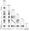 |
Fig. A.2 Corner plot of the fit transit model based on the single transit of K2-141 c in K2 C19 to update the ephemeris of the planet. Gaussian Priors were used on P, a/R*. and cos i based on the values reported in Malavolta et al. (2018) who only used the observations in C12. We used the resulting transit time t0 to recalculate the orbital period P. The transit time in this plot is expressed as BJDTDB - 2458371.0 d. |
Appendix B Additional Tables
Appendix B.1 Rescaling of Uncertainties
χ2 values for each Spitzer AOR before rescaling them to unity.
Appendix B.2 Parameters of the fit Models
All free parameters used in the models which were fit to the Spitzer data alone.
All free parameters used in the models which were fit to the joint Kepler and Spitzer dataset.
Best fit systematic parameters for all six models.
Appendix C Additional Plots
Appendix C.1 Systematics
 |
Fig. C.1 Diagnostic plot of the full Spitzer observations: The vertical, dashed blue lines indicate the start of a new Astronomical Observation Request (AOR). The data in the vertical, gray shaded regions were removed for the fit due to systematic effects. The red line in the top panel shows the best fit model of the Spitzer data. The difference between the model and the normalized flux can be seen in the panel below. The data has been binned downed to 10 minutes in the top two panels and to 4 minutes in the lower panels. The observed raw flux in µJy/pixel is shown in the third panel. The background flux in the fourth panel is showing changes at the beginning of every AOR as expected due to changes in pointing. An outlier segment in AOR5 which was manually removed from the dataset has been able to be attributed to a strong cosmic ray hit on the detector. The 2D images showing this event can be found in Fig. C.2. The parameters, x and y are the pixel position of the target relative to the “sweet spot”. Finally, sx and sy describe the Gaussian widths of the star’s point spread function. |
 |
Fig. C.2 Spitzer data frames showing strong cosmic ray hit on the Spitzer IRAC detector which led to changes in the background flux during AOR5. Each column shows the same Basic Calibrated Data (BCD, provided by the Spitzer Science Center) frame but at a different contrast. The star is located in the center of every frame, whereas the cosmic ray hit can be seen in the lower right of the second frame. All frames in this plot have been taken from the same BCD cube which typically consist out of 64 images with 32 × 32 pixel. |
 |
Fig. C.3 Raw, unbinned light curve is shown with gray dots with the best fitting model in light red. The vertical, dashed blue lines indicate the start of a new Astronomical Observation Request (AOR). The data in the vertical, gray shaded regions were removed for the fit due to systematic effects. The solid black (red) line shows the raw light curve (best fitting model) binned down to 10 minutes. The planetary signatures (transit, phase curve variation or eclipse) are too weak to be seen in the raw data. For example, the transit depth of K2-141 b is ~425 ppm which leads to a dip of just ~30 µJy/pixel. |
 |
Fig. C.4 Reflected and thermal contributions to the total flux in the Kepler and Spitzer bandpasses using our best fitting model (toy model without heat redistribution). The shaded areas show the 1σ uncertainties on the best fitting phase curve shape. The K2 phase curves shown here take the longer exposure time into account (30 minutes for K2 Campaign 12) which leads to a less steep ingress and egress at the eclipse. |
Appendix C.2 Spitzer Pointings
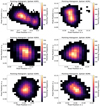 |
Fig. C.5 Pointing diagrams for all six Spitzer AORs. The color map indicates the frequency of exposures for which the centroid of the star hit a certain position. |
Appendix C.3 Spitzer BLISS Maps
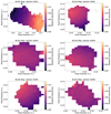 |
Fig. C.6 BLISS sensitivity maps for all six Spitzer AORs. |
Appendix C.4 Spitzer Allan Deviation Plots
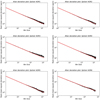 |
Fig. C.7 Allan deviation plots for all six Spitzer AORs. The residuals (black curve) are calculated by taking the difference of the full dataset (Spitzer and Kepler) and the Toy model without redistribution fit. A bin size of one depicts no binning at all. The red line shows the expected root-mean-square (rms) for Gaussian noise following the inverse square root law. |
Appendix C.5 Spitzer Fit: Sinusoidal (ϕ = 0)
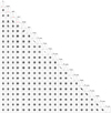 |
Fig. C.8 MCMC corner plot for the sinusoidal model fit without a hotspot offset (ϕ = 0) to the Spitzer data. The red bars for t0, Rp/R*, a/R* and cos i show the Gaussian priors which were used in this fit. The prior values and the best fit values are listed in Table 4. The resulting values for the systematic parameters are in Table B.4. A list with all fit parameters can be found in Table B.2. |
Appendix C.6 Spitzer Fit: Sinusoidal (ϕ free)
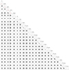 |
Fig. C.9 MCMC corner plot for the sinusoidal model fit with a hotspot offset (ϕ free) to the Spitzer data. The red bars for f0, Rv/R*, a/R, and cos i show the Gaussian priors which were used in this fit. The prior values and the best fit values are listed in Table 4. The resulting values for the systematic parameters are in Table B.4. A list with all fit parameters can be found in Table B.2. |
Appendix C.7 Spitzer Fit: Two Temperature Model
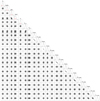 |
Fig. C.10 MCMC corner plot for the two temperature model fit to the Spitzer data. The red bars for t0, Rp/R*, a/R* cos i and T* show the Gaussian priors which were used in this fit. The prior values and the best fit values are listed in Table 4. The resulting values for the systematic parameters are in Table B.4. A list with all fit parameters can be found in Table B.2. |
Appendix C.8 Joint (K2 and Spitzer) Fit: Toy Model (F = 0)
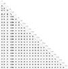 |
Fig. C.11 MCMC corner plot for the toy model fit without heat redistribution (F = 0) to the joint dataset, i.e., Spitzer and K2. The red bars for a/R* and T* show the Gaussian priors which were used in this fit. The prior values and the best fit values are listed in Table 5. The resulting values for the systematic parameters are in Table B.4. A list with all fit parameters can be found in Table B.3. |
Appendix C.9 Joint (K2 and Spitzer) Fit: Toy Model (F Free)
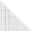 |
Fig. C.12 MCMC corner plot for the toy model fit with heat redistribution (F free) to the joint dataset, i.e., Spitzer and K2. The red bars for a/R* and T* show the Gaussian priors which were used in this fit. The prior values and the best fit values are listed in Table 5. The resulting values for the systematic parameters are in Table B.4. A list with all fit parameters can be found in Table B.3. |
Appendix C.10 Joint (K2 And Spitzer) Fit: Two Temperature Model
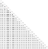 |
Fig. C.13 MCMC corner plot for the two temperature model fit to the joint dataset, i.e., Spitzer and K2. The red bars for a/R* and T* show the Gaussian priors which were used in this fit. The prior values and the best fit values are listed in Table 5. The resulting values for the systematic parameters are in Table B.4. A list with all fit parameters can be found in Table B.3. |
References
- Adams, F. C., & Laughlin, G. 2006, ApJ, 649, 1004 [Google Scholar]
- Allard, F., Allard, N. F., Homeier, D., et al. 2007a, A&A, 474, L21 [NASA ADS] [CrossRef] [EDP Sciences] [Google Scholar]
- Allard, N. F., Kielkopf, J. F., & Allard, F. 2007b, Eur. Phys. J. D, 44, 507 [NASA ADS] [CrossRef] [Google Scholar]
- Angelo, I., & Hu, R. 2017, AJ, 154, 232 [NASA ADS] [CrossRef] [Google Scholar]
- Astropy Collaboration (Robitaille, T. P., et al.) 2013, A&A, 558, A33 [NASA ADS] [CrossRef] [EDP Sciences] [Google Scholar]
- Astropy Collaboration (Price-Whelan, A. M., et al.) 2018, AJ, 156, 123 [Google Scholar]
- Auvergne, M., Bodin, P., Boisnard, L., et al. 2009, A&A, 506, 411 [NASA ADS] [CrossRef] [EDP Sciences] [Google Scholar]
- Barragán, O., Gandolfi, D., Dai, F., et al. 2018, A&A, 612, A95 [Google Scholar]
- Barton, E. J., Yurchenko, S. N., & Tennyson, J. 2013, MNRAS, 434, 1469 [NASA ADS] [CrossRef] [Google Scholar]
- Batalha, N. M., Borucki, W. J., Bryson, S. T., et al. 2011, ApJ, 729, 27 [Google Scholar]
- Batalha, N. E., Mandell, A., Pontoppidan, K., et al. 2017, PASP, 129, 064501 [Google Scholar]
- Borucki, W. J., Koch, D., Basri, G., et al. 2010, Science, 327, 977 [Google Scholar]
- Bourrier, V., Dumusque, X., Dorn, C., et al. 2018, A&A, 619, A1 [NASA ADS] [CrossRef] [EDP Sciences] [Google Scholar]
- Brandeker, A., Alibert, Y., Bourrier, V., et al. 2021, Is it raining lava in the evening on 55 Cancrie?, JWST Proposal. Cycle 1 [Google Scholar]
- Castan, T., & Menou, K. 2011, ApJ, 743, L36 [NASA ADS] [CrossRef] [Google Scholar]
- Challener, R. C., Harrington, J., Jenkins, J., et al. 2021, PSJ, 2, 9 [CrossRef] [Google Scholar]
- Charbonneau, D., Allen, L. E., Megeath, S. T., et al. 2005, ApJ, 626, 523 [Google Scholar]
- Crida, A., Ligi, R., Dorn, C., Borsa, F., & Lebreton, Y. 2018a, RNAAS, 2, 172 [Google Scholar]
- Crida, A., Ligi, R., Dorn, C., & Lebreton, Y. 2018b, ApJ, 860, 122 [NASA ADS] [CrossRef] [Google Scholar]
- Cubillos, P., Harrington, J., Madhusudhan, N., et al. 2013, ApJ, 768, 42 [NASA ADS] [CrossRef] [Google Scholar]
- Dai, F., Masuda, K., Winn, J. N., & Zeng, L. 2019, ApJ, 883, 79 [NASA ADS] [CrossRef] [Google Scholar]
- Dang, L., Cowan, N. B., Hammond, M., et al. 2021, A Hell of a Phase Curve: Mapping the Surface and Atmosphere of a Lava Planet K2-141b, JWST Proposal. Cycle 1 [Google Scholar]
- Dawson, R. I., & Fabrycky, D. C. 2010, ApJ, 722, 937 [Google Scholar]
- Dawson, R. I., & Johnson, J. A. 2018, ARA&A, 56, 175 [Google Scholar]
- Demory, B.-O. 2014, ApJ, 789, L20 [NASA ADS] [CrossRef] [Google Scholar]
- Demory, B. O., Gillon, M., Deming, D., et al. 2011, A&A, 533, A114 [NASA ADS] [CrossRef] [EDP Sciences] [Google Scholar]
- Demory, B.-O., Gillon, M., de Wit, J., et al. 2016a, Nature, 532, 207 [NASA ADS] [CrossRef] [Google Scholar]
- Demory, B.-O., Gillon, M., Madhusudhan, N., & Queloz, D. 2016b, MNRAS, 455, 2018 [NASA ADS] [CrossRef] [Google Scholar]
- Dorn, C., Harrison, J. H. D., Bonsor, A., & Hands, T. O. 2019, MNRAS, 484, 712 [Google Scholar]
- Dumusque, X., Bonomo, A. S., Haywood, R. D., et al. 2014, ApJ, 789, 154 [NASA ADS] [CrossRef] [Google Scholar]
- Espinoza, N., Bello-Arufe, A., Buchhave, L. A., et al. 2021, The first near-infrared spectroscopic phase-curve of a super-Earth, JWST Proposal. Cycle 1 [Google Scholar]
- Essack, Z., Seager, S., & Pajusalu, M. 2020, ApJ, 898, 160 [CrossRef] [Google Scholar]
- Fazio, G. G., Hora, J. L., Allen, L. E., et al. 2004, ApJS, 154, 10 [Google Scholar]
- Fegley, B., & Cameron, A. G. W. 1987, Earth Planet. Sci. Lett., 82, 207 [CrossRef] [Google Scholar]
- Fischer, D. A., Marcy, G. W., Butler, R. P., et al. 2008, ApJ, 675, 790 [Google Scholar]
- Fischer, D. A., & Valenti, J. 2005, ApJ, 622, 1102 [NASA ADS] [CrossRef] [Google Scholar]
- Foreman-Mackey, D. 2016, J. Open Source Softw., 1, 24 [Google Scholar]
- Gelman, A., & Rubin, D. B. 1992, Statist. Sci., 7, 457 [NASA ADS] [Google Scholar]
- Hammond, M., & Pierrehumbert, R. T. 2017, ApJ, 849, 152 [CrossRef] [Google Scholar]
- Harrington, J., Luszcz, S., Seager, S., Deming, D., & Richardson, L. J. 2007, Nature, 447, 691 [NASA ADS] [CrossRef] [Google Scholar]
- Harris, C. R., Millman, K. J., van der Walt, S. J., et al. 2020, Nature, 585, 357 [NASA ADS] [CrossRef] [Google Scholar]
- Howell, S. B., Sobeck, C., Haas, M., et al. 2014, PASP, 126, 398 [Google Scholar]
- Hu, R., Demory, B.-O., Seager, S., Lewis, N., & Showman, A. P. 2015, ApJ, 802, 51 [Google Scholar]
- Hu, R., Brandeker, A., Damiano, M., et al. 2021, Determining the Atmospheric Composition of the Super-Earth 55 Cancri e, JWST Proposal. Cycle 1 [Google Scholar]
- Hunter, J. D. 2007, Comput. Sci. Eng., 9, 90 [NASA ADS] [CrossRef] [Google Scholar]
- Husser, T. O., Wende-von Berg, S., Dreizler, S., et al. 2013, A&A, 553, A6 [NASA ADS] [CrossRef] [EDP Sciences] [Google Scholar]
- Ito, Y., Ikoma, M., Kawahara, H., et al. 2015, ApJ, 801, 144 [NASA ADS] [CrossRef] [Google Scholar]
- Jackson, B., Stark, C. C., Adams, E. R., Chambers, J., & Deming, D. 2013, ApJ, 779, 165 [NASA ADS] [CrossRef] [Google Scholar]
- Kass, R. E., & Raftery, A. E. 1995, J. Am. Stat. Assoc., 90, 773 [Google Scholar]
- Kipping, D., & Jansen, T. 2020, RNAAS, 4, 170 [NASA ADS] [Google Scholar]
- Kite, E. S., Fegley Bruce, J., Schaefer, L., & Gaidos, E. 2016, ApJ, 828, 80 [NASA ADS] [CrossRef] [Google Scholar]
- Koll, D. D. B., Malik, M., Mansfield, M., et al. 2019, ApJ, 886, 140 [NASA ADS] [CrossRef] [Google Scholar]
- Kopal, Z. 1954, MNRAS, 114, 101 [NASA ADS] [CrossRef] [Google Scholar]
- Kreidberg, L. 2015, PASP, 127, 1161 [Google Scholar]
- Kreidberg, L., & Loeb, A. 2016, ApJ, 832, L12 [NASA ADS] [CrossRef] [Google Scholar]
- Kreidberg, L., Lopez, E., Cowan, N., et al. 2018, Taking the Temperature of a Lava Planet, Spitzer Proposal [Google Scholar]
- Kreidberg, L., Koll, D. D. B., Morley, C., et al. 2019, Nature, 573, 87 [NASA ADS] [CrossRef] [Google Scholar]
- Kreidberg, L., Hu, R., Kite, E. S., et al. 2021, A Search for Signatures of Volcanism and Geodynamics on the Hot Rocky Exoplanet LHS 3844b, JWST Proposal. Cycle 1 [Google Scholar]
- Kurucz, R. L. 1992, Rev. Mexicana Astron. Astrofis., 23, 45 [Google Scholar]
- Kurucz, R. L. 1993, SYNTHE spectrum synthesis programs and line data [Google Scholar]
- Lanotte, A. A., Gillon, M., Demory, B. O., et al. 2014, A&A, 572, A73 [NASA ADS] [CrossRef] [EDP Sciences] [Google Scholar]
- Léger, A., Grasset, O., Fegley, B., et al. 2011, Icarus, 213, 1 [CrossRef] [Google Scholar]
- Liddle, A. R. 2007, MNRAS, 377, L74 [NASA ADS] [Google Scholar]
- Lightkurve Collaboration, Cardoso, J. V. D. M., Hedges, C., et al. 2018, Astrophysics Source Code Library [record ascl:1812.013] [Google Scholar]
- Lopez, E. D. 2017, MNRAS, 472, 245 [NASA ADS] [CrossRef] [Google Scholar]
- Louden, T., & Kreidberg, L. 2018, MNRAS, 477, 2613 [NASA ADS] [CrossRef] [Google Scholar]
- Lundkvist, M. S., Kjeldsen, H., Albrecht, S., et al. 2016, Nat. Commun., 7, 11201 [Google Scholar]
- Lust, N. B., Britt, D., Harrington, J., et al. 2014, PASP, 126, 1092 [NASA ADS] [CrossRef] [Google Scholar]
- Malavolta, L., Mayo, A. W., Louden, T., et al. 2018, AJ, 155, 107 [NASA ADS] [CrossRef] [Google Scholar]
- Malik, M., Grosheintz, L., Mendonça, J. M., et al. 2017, AJ, 153, 56 [Google Scholar]
- Malik, M., Kitzmann, D., Mendonça, J. M., et al. 2019, AJ, 157, 170 [Google Scholar]
- Mandel, K., & Agol, E. 2002, ApJ, 580, L171 [Google Scholar]
- May, E. M., & Stevenson, K. B. 2020, AJ, 160, 140 [NASA ADS] [CrossRef] [Google Scholar]
- Mayorga, L. C., Jackiewicz, J., Rages, K., et al. 2016, AJ, 152, 209 [NASA ADS] [CrossRef] [Google Scholar]
- McEwen, A. S., Keszthelyi, L., Spencer, J. R., et al. 1998, Science, 281, 87 [NASA ADS] [CrossRef] [Google Scholar]
- Mendonça, J. M., Malik, M., Demory, B.-O., & Heng, K. 2018, AJ, 155, 150 [Google Scholar]
- Miguel, Y., Kaltenegger, L., Fegley, B., & Schaefer, L. 2011, ApJ, 742, L19 [NASA ADS] [CrossRef] [Google Scholar]
- Modirrousta-Galian, D., Ito, Y., & Micela, G. 2021, Icarus, 358, 114175 [CrossRef] [Google Scholar]
- Mollière, P., Wardenier, J. P., van Boekel, R., et al. 2019, A&A, 627, A67 [Google Scholar]
- Morris, B. M., Delrez, L., Brandeker, A., et al. 2021, A&A, 653, A173 [NASA ADS] [CrossRef] [EDP Sciences] [Google Scholar]
- Nguyen, T. G., Cowan, N. B., Banerjee, A., & Moores, J. E. 2020, MNRAS, 499, 4605 [NASA ADS] [CrossRef] [Google Scholar]
- Nguyen, T. G., Cowan, N., Pierrehumbert, R., Lupu, R., & Moores, J. 2022, MNRAS, in press [Google Scholar]
- Perez, F., & Granger, B. E. 2007, Comput. Sci. Eng., 9, 21 [Google Scholar]
- Pont, F., Zucker, S., & Queloz, D. 2006, MNRAS, 373, 231 [NASA ADS] [CrossRef] [Google Scholar]
- Ricker, G. R., Winn, J. N., Vanderspek, R., et al. 2014, SPIE Conf. Ser., 9143, 914320 [Google Scholar]
- Rossi, F., & Pascale, J. 1985, Phys. Rev. A, 32, 2657 [CrossRef] [Google Scholar]
- Rouan, D., Deeg, H. J., Demangeon, O., et al. 2011, ApJ, 741, L30 [Google Scholar]
- Ryabchikova, T., Piskunov, N., Kurucz, R. L., et al. 2015, Phys. Scr, 90, 054005 [Google Scholar]
- Sanchis-Ojeda, R., Rappaport, S., Winn, J. N., et al. 2013, ApJ, 774, 54 [Google Scholar]
- Sanchis-Ojeda, R., Rappaport, S., Winn, J. N., et al. 2014, ApJ, 787, 47 [Google Scholar]
- Schaefer, L., & Fegley, B. 2004, Icarus, 169, 216 [CrossRef] [Google Scholar]
- Schaefer, L., & Fegley, B. 2010, Icarus, 208, 438 [NASA ADS] [CrossRef] [Google Scholar]
- Schwarz, G. 1978, Ann. Statist., 6, 461 [Google Scholar]
- Seager, S. 2010, Exoplanet Atmospheres: Physical Processes [Google Scholar]
- Sheets, H. A., & Deming, D. 2014, ApJ, 794, 133 [NASA ADS] [CrossRef] [Google Scholar]
- Showman, A. P., & Polvani, L. M. 2011, ApJ, 738, 71 [Google Scholar]
- Singh, V., Bonomo, A. S., Scandariato, G., et al. 2022, A&A, 658, A132 [NASA ADS] [CrossRef] [EDP Sciences] [Google Scholar]
- Speagle, J. S. 2020, MNRAS, 493, 3132 [Google Scholar]
- Stevenson, K. B., Harrington, J., Fortney, J. J., et al. 2012, ApJ, 754, 136 [Google Scholar]
- Stock, J.W., Kitzmann, D., Patzer, A. B. C., & Sedlmayr, E. 2018, MNRAS, 479, 865 [NASA ADS] [Google Scholar]
- Sulis, S., Dragomir, D., Lendl, M., et al. 2019, A&A, 631, A129 [NASA ADS] [CrossRef] [EDP Sciences] [Google Scholar]
- Tamburo, P., Mandell, A., Deming, D., & Garhart, E. 2018, AJ, 155, 221 [NASA ADS] [CrossRef] [Google Scholar]
- Ter Braak, C. J. F. 2006, Stat. Comput., 16, 239 [Google Scholar]
- Van Eylen, V., Agentoft, C., Lundkvist, M. S., et al. 2018, MNRAS, 479, 4786 [Google Scholar]
- Vanderburg, A., & Johnson, J. A. 2014, PASP, 126, 948 [Google Scholar]
- Vanderburg, A., Latham, D. W., Buchhave, L. A., et al. 2016, ApJS, 222, 14 [Google Scholar]
- Vanderburg, A., Becker, J. C., Buchhave, L. A., et al. 2017, AJ, 154, 237 [NASA ADS] [CrossRef] [Google Scholar]
- Vanderspek, R., Huang, C. X., Vanderburg, A., et al. 2019, ApJ, 871, L24 [Google Scholar]
- Virtanen, P., Gommers, R., Oliphant, T. E., et al. 2020, Nature Methods, 17, 261 [CrossRef] [Google Scholar]
- Winn, J. N., Holman, M. J., Bakos, G. Á., et al. 2007, AJ, 134, 1707 [NASA ADS] [CrossRef] [Google Scholar]
- Winn, J. N., Holman, M. J., Torres, G., et al. 2008, ApJ, 683, 1076 [Google Scholar]
- Winn, J. N., Matthews, J. M., Dawson, R. I., et al. 2011, ApJ, 737, L18 [Google Scholar]
- Winn, J. N., Sanchis-Ojeda, R., Rogers, L., et al. 2017, AJ, 154, 60 [NASA ADS] [CrossRef] [Google Scholar]
- Winn, J. N., Sanchis-Ojeda, R., & Rappaport, S. 2018, New A Rev., 83, 37 [Google Scholar]
- Zeng, L., Jacobsen, S. B., Sasselov, D. D., et al. 2019, Proc. Natl. Acad. Sci. U.S.A., 116, 9723 [Google Scholar]
- Zhang, M., Dai, F., Hu, R., Knutson, H. A., & Lam, K. 2021, The First and Only Multi-wavelength Map of an Ultra-short-period sub-Earth, JWST Proposal. Cycle 1 [Google Scholar]
- Zilinskas, M., Miguel, Y., Lyu, Y., & Bax, M. 2021, MNRAS, 500, 2197 [Google Scholar]
- Zilinskas, M., van Buchem, C., Miguel, Y., et al. 2022, A&A, 661, A126 [NASA ADS] [CrossRef] [EDP Sciences] [Google Scholar]
Calculated using  while assuming Bond albedo AB = 0. The heat redistribution factor, f, is f = 1/4 in case of uniform redistribution (if the planet has a thick atmosphere able to redistribute heat) and f = 2/3 for instant reradiation (if the planet is a bare rock) (Koll et al. 2019).
Calculations based on the Mass-Radius tables from Zeng et al. (2019).
Calculations based on Kopal (1954) and Nguyen et al. (2020).
The star was proposed to be observed in short cadence mode in K2 Campaign 19 from the following K2 General Observer programs: GO19027, A. Vanderburg; GO19065, C. Dressing.
See the Data Release Notes for K2 Campaign 19 for further information: https://archive.stsci.edu/missions/k2/doc/drn/KSCI-19145-882_K2-DRN29_C19.pdf
Komatiites are magnesium-rich, ultramafic lavas which formed on Earth during the Archaean (3.8–2.5 billion years ago) when the Earth had higher surface temperatures (McEwen et al. 1998; Schaefer & Fegley 2004).
All Tables
Parameters used for the data reduction of every Spitzer AOR determined by minimizing the Bayesian Information Criterion (BIC).
Updated ephemeris for K2-141 b and the 3tr uncertainty on the predicted transit time in 2022 and 2024.
Updated ephemeris for K2-141 c and the 3σ uncertainty on the predicted transit time in 2022 and 2024.
All free parameters used in the models which were fit to the joint Kepler and Spitzer dataset.
All Figures
 |
Fig. 1 Phase curve of K2-141 b after phase folding the complete Spitzer observations. The eclipse is at phase = 0.5. The best fitting model shown in red describes the observed thermal emission from the planet as a sinusoidal function. Each bin in black (gray) consists out of 7200 (1800) Spitzer 2-s exposures. The pairs plot for this model can be found in the Appendix C.5. |
| In the text | |
 |
Fig. 2 Allan deviation plot of the Spitzer data: root-mean-square (rms) of the fit residuals of the Spitzer data using the sinusoidal model without a hotspot offset (black curve) as a function of the number of data points per bin. A bin size of one depicts no binning at all. The red line shows the expected rms for Gaussian noise following the inverse square root law. |
| In the text | |
 |
Fig. 3 Allan deviation plot for K2 C12 in the left panel and K2 C19 in the right panel. |
| In the text | |
 |
Fig. 4 K2 Campaign 19 data of K2-141. Upper panel: the full K2 Campaign 19 observations. We removed outliers and data suffering from decreased photometric precision due to Kepler running out of fuel (marked in orange). Middle panel: K2 C19 data with instrumental systematics removed using the SFF algorithm. Lower panel: the K2 C19 observations after removal of the stellar variability. The 25 transits by K2-141 b have been marked in green. An additional transit by K2-141 c is denoted in red. |
| In the text | |
 |
Fig. 5 Corner plot of the best fitting model to the joint K2 and Spitzer dataset for the dayside temperature Tp,d, the nightside temperature Tp,n and the geometric albedo Ag. |
| In the text | |
 |
Fig. 6 Phase curve of K2-141 b as seen by Kepler during Campaign 12 and 19. Upper panel: the solid black line shows the phase curve based on the values in our best fit model (toy model without heat redistribution for the thermal emission and a uniform Lambertian reflector for the reflected light contribution). The dark orange and light orange areas around the best fitting model are the 1σ and 3σ uncertainties, respectively. We binned the Campaign 19 data that was collected in short cadence mode (~1 min) into bins of 29.4 min to have the same temporal resolution as the Campaign 12 data. We then phase folded the Kepler observations and binned the data for clarity. Each bin in black (gray) consists out of 180 (45) Kepler exposures. Lower panel: the residuals of the Kepler observations to the best fitting model. |
| In the text | |
 |
Fig. 7 T–P profile of K2-141 b based on the pseudo-2D rock vapor model as described in Sect. 4.1 at different angles from the substellar point. |
| In the text | |
 |
Fig. 8 Column density of various species as a function of the zenith angle of the planet for a Bulk-Silicate-Earth composition (left panel) and a komitiite composition (right panel) based on calculations in Miguel et al. (2011). The temperature as a function of zenith angle assumed for this plot is based on the our best fit model presented in Kreidberg & Loeb (2016) without heat redistribution (F = 0). It assumes that the temperature at the substellar point is |
| In the text | |
 |
Fig. 9 Surface pressure as a function of the zenith angle for the two different models used in this paper. The dashed pink line is based on the pseudo-2D rock vapor model and the blue lines are based on the 1D TBL model for a Na, SiO and SiO2 atmosphere. Although, the TBL models shown in this plot are based on Nguyen et al. (2020) and lack radiative transfer, this would introduce little to no changes to the surface pressure. Na is the most volatile possible component of rock vapor atmosphere, so a pure Na atmosphere has the highest surface pressure (Schaefer & Fegley 2004). |
| In the text | |
 |
Fig. 10 Eclipse depths measured in the Kepler and Spitzer bandpasses compared to different emission spectra of the planet: the pink solid line was calculated using the pseudo-2D rock vapor model and shows thermal emissions in the optical due to Na. The dashed orange line uses the best fit dayside temperature Tp,d and geometric albedo Ag values using the joint dataset (Spitzer & K2). The orange shaded area is due to the uncertainties in Tp,d and Ag. We also show black body (BB) emission spectra in gray for two exemplary dayside temperatures of K2-141 b assuming a geometric albedo of Ag = 0: Tp,d = 2150K that corresponds to a full redistribution of heat on the planet (whole planet is isothermal) and Tp,d = 2745 K in case of instant reradiation of incoming energy (nightside temperature is zero). Any features in the black body spectra are originating from the host star because we divide the black body spectrum of the planet with a Kurucz stellar spectrum (Kurucz 1993). The pink (orange) boxes show the Spitzer and K2 bandpass integrated eclipse depth for the rock vapor model (sum of the thermal and reflective emission from the best fit to the joint data set). |
| In the text | |
 |
Fig. 11 Observed Spitzer phase curve and the best fit sine curve to the Spitzer data (red dashed line with the one sigma uncertainty shaded in red) compared to four theoretical phase curves: the different three blue solid lines are phase curves for the 1D TBL model assuming an adiabatic, an isothermal and an temperature inversion case. We also generated a phase curve out of the pseudo-2D rock vapor model (solid pink line). The adiabatic, isothermal and rock vapor model all fit the observations well and the temperature inversion model provides the worst fit. |
| In the text | |
 |
Fig. 12 Eclipse depth of Kepler-10 b measured in the Kepler bandpass compared to a pseudo-2D rock vapor model in pink showing emission features caused by thermal emission. The pink square is the predicted bandpass integrated eclipse depth assuming the rock vapor atmosphere model for the planet. |
| In the text | |
 |
Fig. A.1 The transit of K2-141 c in C19 with 100 random draws from the posterior in red. |
| In the text | |
 |
Fig. A.2 Corner plot of the fit transit model based on the single transit of K2-141 c in K2 C19 to update the ephemeris of the planet. Gaussian Priors were used on P, a/R*. and cos i based on the values reported in Malavolta et al. (2018) who only used the observations in C12. We used the resulting transit time t0 to recalculate the orbital period P. The transit time in this plot is expressed as BJDTDB - 2458371.0 d. |
| In the text | |
 |
Fig. C.1 Diagnostic plot of the full Spitzer observations: The vertical, dashed blue lines indicate the start of a new Astronomical Observation Request (AOR). The data in the vertical, gray shaded regions were removed for the fit due to systematic effects. The red line in the top panel shows the best fit model of the Spitzer data. The difference between the model and the normalized flux can be seen in the panel below. The data has been binned downed to 10 minutes in the top two panels and to 4 minutes in the lower panels. The observed raw flux in µJy/pixel is shown in the third panel. The background flux in the fourth panel is showing changes at the beginning of every AOR as expected due to changes in pointing. An outlier segment in AOR5 which was manually removed from the dataset has been able to be attributed to a strong cosmic ray hit on the detector. The 2D images showing this event can be found in Fig. C.2. The parameters, x and y are the pixel position of the target relative to the “sweet spot”. Finally, sx and sy describe the Gaussian widths of the star’s point spread function. |
| In the text | |
 |
Fig. C.2 Spitzer data frames showing strong cosmic ray hit on the Spitzer IRAC detector which led to changes in the background flux during AOR5. Each column shows the same Basic Calibrated Data (BCD, provided by the Spitzer Science Center) frame but at a different contrast. The star is located in the center of every frame, whereas the cosmic ray hit can be seen in the lower right of the second frame. All frames in this plot have been taken from the same BCD cube which typically consist out of 64 images with 32 × 32 pixel. |
| In the text | |
 |
Fig. C.3 Raw, unbinned light curve is shown with gray dots with the best fitting model in light red. The vertical, dashed blue lines indicate the start of a new Astronomical Observation Request (AOR). The data in the vertical, gray shaded regions were removed for the fit due to systematic effects. The solid black (red) line shows the raw light curve (best fitting model) binned down to 10 minutes. The planetary signatures (transit, phase curve variation or eclipse) are too weak to be seen in the raw data. For example, the transit depth of K2-141 b is ~425 ppm which leads to a dip of just ~30 µJy/pixel. |
| In the text | |
 |
Fig. C.4 Reflected and thermal contributions to the total flux in the Kepler and Spitzer bandpasses using our best fitting model (toy model without heat redistribution). The shaded areas show the 1σ uncertainties on the best fitting phase curve shape. The K2 phase curves shown here take the longer exposure time into account (30 minutes for K2 Campaign 12) which leads to a less steep ingress and egress at the eclipse. |
| In the text | |
 |
Fig. C.5 Pointing diagrams for all six Spitzer AORs. The color map indicates the frequency of exposures for which the centroid of the star hit a certain position. |
| In the text | |
 |
Fig. C.6 BLISS sensitivity maps for all six Spitzer AORs. |
| In the text | |
 |
Fig. C.7 Allan deviation plots for all six Spitzer AORs. The residuals (black curve) are calculated by taking the difference of the full dataset (Spitzer and Kepler) and the Toy model without redistribution fit. A bin size of one depicts no binning at all. The red line shows the expected root-mean-square (rms) for Gaussian noise following the inverse square root law. |
| In the text | |
 |
Fig. C.8 MCMC corner plot for the sinusoidal model fit without a hotspot offset (ϕ = 0) to the Spitzer data. The red bars for t0, Rp/R*, a/R* and cos i show the Gaussian priors which were used in this fit. The prior values and the best fit values are listed in Table 4. The resulting values for the systematic parameters are in Table B.4. A list with all fit parameters can be found in Table B.2. |
| In the text | |
 |
Fig. C.9 MCMC corner plot for the sinusoidal model fit with a hotspot offset (ϕ free) to the Spitzer data. The red bars for f0, Rv/R*, a/R, and cos i show the Gaussian priors which were used in this fit. The prior values and the best fit values are listed in Table 4. The resulting values for the systematic parameters are in Table B.4. A list with all fit parameters can be found in Table B.2. |
| In the text | |
 |
Fig. C.10 MCMC corner plot for the two temperature model fit to the Spitzer data. The red bars for t0, Rp/R*, a/R* cos i and T* show the Gaussian priors which were used in this fit. The prior values and the best fit values are listed in Table 4. The resulting values for the systematic parameters are in Table B.4. A list with all fit parameters can be found in Table B.2. |
| In the text | |
 |
Fig. C.11 MCMC corner plot for the toy model fit without heat redistribution (F = 0) to the joint dataset, i.e., Spitzer and K2. The red bars for a/R* and T* show the Gaussian priors which were used in this fit. The prior values and the best fit values are listed in Table 5. The resulting values for the systematic parameters are in Table B.4. A list with all fit parameters can be found in Table B.3. |
| In the text | |
 |
Fig. C.12 MCMC corner plot for the toy model fit with heat redistribution (F free) to the joint dataset, i.e., Spitzer and K2. The red bars for a/R* and T* show the Gaussian priors which were used in this fit. The prior values and the best fit values are listed in Table 5. The resulting values for the systematic parameters are in Table B.4. A list with all fit parameters can be found in Table B.3. |
| In the text | |
 |
Fig. C.13 MCMC corner plot for the two temperature model fit to the joint dataset, i.e., Spitzer and K2. The red bars for a/R* and T* show the Gaussian priors which were used in this fit. The prior values and the best fit values are listed in Table 5. The resulting values for the systematic parameters are in Table B.4. A list with all fit parameters can be found in Table B.3. |
| In the text | |
Current usage metrics show cumulative count of Article Views (full-text article views including HTML views, PDF and ePub downloads, according to the available data) and Abstracts Views on Vision4Press platform.
Data correspond to usage on the plateform after 2015. The current usage metrics is available 48-96 hours after online publication and is updated daily on week days.
Initial download of the metrics may take a while.


