| Issue |
A&A
Volume 679, November 2023
|
|
|---|---|---|
| Article Number | A92 | |
| Number of page(s) | 17 | |
| Section | Planets and planetary systems | |
| DOI | https://doi.org/10.1051/0004-6361/202244946 | |
| Published online | 16 November 2023 | |
CHEOPS and TESS view of the ultra-short-period super-Earth TOI-561 b★,★★
1
Department of Astronomy, Stockholm University, AlbaNova University Center,
10691
Stockholm, Sweden
e-mail: This email address is being protected from spambots. You need JavaScript enabled to view it.
2
Physikalisches Institut, University of Bern,
Gesellschaftsstrasse 6,
3012
Bern, Switzerland
3
Centre for Exoplanet Science, SUPA School of Physics and Astronomy, University of St Andrews,
North Haugh,
St Andrews
KY16 9SS, UK
4
Department of Physics, University of Warwick,
Gibbet Hill Road,
Coventry
CV4 7AL, UK
5
Observatoire Astronomique de l’Université de Genève,
Chemin Pegasi 51,
1290
Versoix, Switzerland
6
Space Research Institute, Austrian Academy of Sciences,
Schmiedlstrasse 6,
8042
Graz, Austria
7
Centre Vie dans l’Univers, Faculté des sciences, Université de Genève,
Quai Ernest-Ansermet 30,
1211
Genève 4, Switzerland
8
Instituto de Astrofisica e Ciencias do Espaco, Universidade do Porto, CAUP,
Rua das Estrelas,
4150-762
Porto, Portugal
9
Center for Space and Habitability, University of Bern,
Gesellschaftsstrasse 6,
3012
Bern, Switzerland
10
Institute of Planetary Research, German Aerospace Center (DLR),
Rutherfordstrasse 2,
12489
Berlin, Germany
11
Instituto de Astrofisica de Canarias,
38200
La Laguna, Tenerife, Spain
12
Departamento de Astrofisica, Universidad de La Laguna,
38206
La Laguna, Tenerife, Spain
13
Institut de Ciencies de l’Espai (ICE, CSIC),
Campus UAB, Can Magrans s/n,
08193
Bellaterra, Spain
14
Institut d’Estudis Espacials de Catalunya (IEEC),
08034
Barcelona, Spain
15
Admatis,
5. Kandó Kálmán Street,
3534
Miskolc, Hungary
16
Depto. de Astrofisica, Centro de Astrobiología (CSIC-INTA),
ESAC campus,
28692
Villanueva de la Cañada (Madrid), Spain
17
Departamento de Fisica e Astronomia, Faculdade de Ciencias, Universidade do Porto,
Rua do Campo Alegre,
4169-007
Porto, Portugal
18
Université Grenoble Alpes, CNRS, IPAG,
38000
Grenoble, France
19
Université de Paris, Institut de physique du globe de Paris, CNRS,
75005
Paris, France
20
Centre for Mathematical Sciences, Lund University,
Box 118,
221 00
Lund, Sweden
21
Aix-Marseille Univ, CNRS, CNES, LAM,
38 rue Frédéric Joliot-Curie,
13388
Marseille, France
22
Astrobiology Research Unit, Université de Liège,
Allée du Six-Août 19C,
4000
Liège, Belgium
23
Space sciences, Technologies and Astrophysics Research (STAR) Institute, Université de Liège,
Allée du Six-Août 19C,
4000
Liège, Belgium
24
Leiden Observatory, University of Leiden,
PO Box 9513,
2300 RA
Leiden, The Netherlands
25
Department of Space, Earth and Environment, Chalmers University of Technology, Onsala Space Observatory,
439 92
Onsala, Sweden
26
Dipartimento di Fisica, Universita degli Studi di Torino,
via Pietro Giuria 1,
10125,
Torino, Italy
27
Department of Astrophysics, University of Vienna,
Türkenschanzstrasse 17,
1180
Vienna, Austria
28
Science and Operations Department - Science Division (SCI-SC), Directorate of Science, European Space Agency (ESA), European Space Research and Technology Centre (ESTEC),
Keplerlaan 1,
2201-AZ
Noordwijk, The Netherlands
29
Konkoly Observatory, Research Centre for Astronomy and Earth Sciences,
1121
Budapest,
Konkoly Thege Miklós út 15-17, Hungary
30
ELTE Eötvös Loránd University, Institute of Physics,
Pázmány Péter sétány 1/A,
1117
Budapest, Hungary
31
Institute of Optical Sensor Systems, German Aerospace Center (DLR),
Rutherfordstrasse 2,
12489
Berlin, Germany
32
IMCCE, UMR8028 CNRS, Observatoire de Paris, PSL Univ., Sorbonne Univ.,
77 av. Denfert-Rochereau,
75014
Paris, France
33
Institut d’astrophysique de Paris, UMR7095 CNRS, Université Pierre & Marie Curie,
98bis Bd Arago,
75014
Paris, France
34
INAF, Osservatorio Astronomico di Padova,
Vicolo dell’Osservatorio 5,
35122
Padova, Italy
35
Astrophysics Group, Keele University,
Staffordshire,
ST5 5BG, UK
36
INAF, Osservatorio Astrofisico di Catania,
Via S. Sofia 78,
95123
Catania, Italy
37
Dipartimento di Fisica e Astronomia “Galileo Galilei”, Università degli Studi di Padova,
Vicolo dell’Osservatorio 3,
35122
Padova, Italy
38
ETH Zurich, Department of Physics,
Wolfgang-Pauli-Strasse 2,
8093
Zurich, Switzerland
39
Cavendish Laboratory,
JJ Thomson Avenue,
Cambridge
CB3 0HE, UK
40
ESTEC, European Space Agency,
2201 AZ,
Noordwijk, The Netherlands
41
Zentrum für Astronomie und Astrophysik, Technische Universität Berlin,
Hardenbergstr. 36,
10623
Berlin, Germany
42
Institut für Geologische Wissenschaften, Freie Universität Berlin,
12249
Berlin, Germany
43
ELTE Eötvös Loránd University, Gothard Astrophysical Observatory,
9700
Szombathely,
Szent Imre h. u. 112, Hungary
44
MTA-ELTE Exoplanet Research Group,
9700
Szombathely,
Szent Imre h. u. 112, Hungary
45
Institute of Astronomy, University of Cambridge,
Madingley Road,
Cambridge,
CB3 0HA, UK
Received:
9
September
2022
Accepted:
14
August
2023
Abstract
Context. Ultra-short-period planets (USPs) are a unique class of super-Earths with an orbital period of less than a day, and hence they are subject to intense radiation from their host star. These planets cannot retain a primordial H/He atmosphere, and most of them are indeed consistent with being bare rocky cores. A few USPs, however, show evidence for a heavyweight envelope, which could be a water layer resilient to evaporation or a secondary metal-rich atmosphere sustained by outgassing of the molten volcanic surface. Much thus remains to be learned about the nature and formation of USPs.
Aims. The prime goal of the present work is to refine the bulk planetary properties of the recently discovered TOI-561 b through the study of its transits and occultations. This is crucial in order to understand the internal structure of this USP and to assess the presence of an atmosphere.
Methods. We obtained ultra-precise transit photometry of TOI-561 b with CHEOPS, and performed a joint analysis of these data along with three archival visits from CHEOPS and four TESS sectors.
Results. Our analysis of TOI-561 b transit photometry put strong constraints on its properties. In particular, we restrict the uncertainties on the planetary radius at ~2% retrieving Rp = 1.42 ± 0.02 R⊕. This result informs our internal structure modelling of the planet, which shows that the observations are consistent with a negligible H/He atmosphere; however, other lighter materials are required, in addition to a pure iron core and a silicate mantle, to explain the observed density. We find that this can be explained by the inclusion of a water layer in our model. Additionally, we ran a grid of forward models with a water-enriched atmosphere to explain the transit radius. We searched for variability in the measured Rp/R★ over time, which could trace changes in the structure of the planetary envelope. However, no temporal variations are recovered within the present data precision. In addition to the transit event, we tentatively detect an occultation signal in the TESS data with an eclipse depth L = 27.40−11.35+10.87 ppm. We use models of outgassed atmospheres from the literature to explain this eclipse signal. We find that the thermal emission from the planet can mostly explain the observation. Based on this, we predict that near- to mid-infrared observations with the James Webb Space Telescope should be able to detect silicate species in the atmosphere of the planet. This could also reveal important clues about the planetary interior and help disentangle planet formation and evolution models.
Key words: techniques: photometric / planets and satellites: terrestrial planets / planets and satellites: composition / planets and satellites: atmospheres / planets and satellites: individual: TOI-561 b
The raw and detrended photometric time series data are available at the CDS via anonymous ftp to cdsarc.cds.unistra.fr (130.79.128.5) or via https://cdsarc.cds.unistra.fr/viz-bin/cat/J/A+A/679/A92
Based in part on Guaranteed Time Observations on the European Space Agency telescope CHEOPS under programme 10.0008 by the CHEOPS Consortium.
© The Authors 2023
 Open Access article, published by EDP Sciences, under the terms of the Creative Commons Attribution License (https://creativecommons.org/licenses/by/4.0), which permits unrestricted use, distribution, and reproduction in any medium, provided the original work is properly cited.
This article is published in open access under the Subscribe to Open model. This email address is being protected from spambots. You need JavaScript enabled to view it. to support open access publication.
1 Introduction
The advent of the new generation of exoplanet discovery missions, such as Kepler/K2 (Borucki et al. 2010; Howell et al. 2014) and the Transiting Exoplanet Survey Satellite (TESS; Ricker et al. 2014), has led to the detection of the vast majority of the known exoplanets. These planets and planetary systems show a large diversity in terms of composition and orbital architecture. In particular one curious class of lower mass planets exists with radius smaller than ~2R⊕ and that orbit the host star within a day, and hence are called ultra-short-period planets (USPs; see Winn et al. 2018, for a review). USPs receive extreme radiation from their host stars, leading to the loss of any primary H/He atmosphere these planets may have formed with (Lopez & Fortney 2013; Owen & Wu 2013, 2016). However, these planets could develop and sustain secondary atmospheres made of heavier species. This may consist of a variety of species such as Na, K, SiO, SiO2, and O2, depending upon the dayside temperature and pressure (Schaefer & Fegley 2009; Miguel et al. 2011; Schaefer et al. 2012; Wordsworth & Kreidberg 2022). Since the surface of the planet can potentially be molten (Léger et al. 2011), the composition of the atmosphere becomes strongly dependent on that of the interior (see e.g. Wordsworth & Kreidberg 2022). The temperature gradient across the day- and night-side of the planet can transport some of the species to the night-side, causing their condensation (Kite et al. 2016). Additionally, some of the species can be lost into space (see Wordsworth & Kreidberg 2022, for a review). These various processes could potentially result in temporal variability for the atmosphere of some USPs (Kite et al. 2016). In the most extreme cases the surface of the planet itself is thought to be disintegrating and escaping into space, leading to the formation of dust tails that can be observed through their highly asymmetric transit light curves (see e.g. Rappaport et al. 2012, 2014; Brogi et al. 2012). The photometric and spectroscopic observations of such disintegrating planets, and more generally of USPs, not only give insights into the nature of their atmospheres, but also provide essential clues regarding their interiors.
The formation mechanism of USPs is a topic of active research. The scarcity of close-in planets with sub-Jovian mass in the Neptunian desert (e.g. Lecavelier des Etangs 2007; Davis & Wheatley 2009; Szabó & Kiss 2011; Beaugé & Nesvorný 2013; Lundkvist et al. 2016), which is thought to be a result of atmospheric escape (e.g. Lecavelier des Etangs et al. 2004; Owen & Jackson 2012; Owen 2019), led to a conjecture that the USPs are remnants of hot Neptunes that have gone through strong mass loss (e.g. Ehrenreich & Désert 2011; Lopez & Fortney 2013; Venturini et al. 2020). Furthermore, Winn et al. (2017) show that the metallicity distribution of USP hosts is very similar to that of mini-Neptune hosts, which supports the suggested formation pathway. Other hypotheses proposed to explain the formation of USPs include the migration of rocky planets from outer orbits and in situ formation (Raymond et al. 2008; Winn et al. 2018).
In order to better understand the formation mechanism of USPs and to constrain their internal structure and atmospheric composition, it is important to perform systematic studies refining their mass and radius. TESS, with its whole sky survey mode for exoplanet discovery, is a unique instrument for discovering new USPs around nearby stars. Weiss et al. (2021) and Lacedelli et al. (2021) have uncovered a multiplanetary system around a small metal-poor G-dwarf, TOI-561, which contains a USP, TOI-561 b, by analysing two TESS sectors along with other follow-up observations. Being a kinematic and chemically thick disk star, TOI-561 is alpha-enhanced (Lacedelli et al. 2022). This means that composition of the protoplanetary disk is likely different to those around solar-metallicity stars. This chemical diversity is likely propagated through to planetary internal structures (Asplund et al. 2009; Thiabaud et al. 2014), as is starting to be seen observationally (Adibekyan et al. 2021; Chen et al. 2022; Wilson et al. 2022). This could make the core of the planets it hosts smaller and the silicate mantle larger. This, in addition to a potentially volatile envelope, is likely one of the main reasons why TOI-561 b is the lowest density USP observed to date. The low density composition (0.69ρ⊕, Lacedelli et al. 2022) is drastically different from other well-known USPs, such as 55 Cnc e or K2-141 b, which have much higher densities (1.21 ρ⊕ and 1.48 ρ⊕, respectively; Bourrier et al. 2018; Malavolta et al. 2018). This makes TOI-561 b an interesting target for follow-up observations.
Among the multiple planets hosted by TOI-561, the innermost planet was found to orbit the star in just ~11 h. To probe the nature of this extremely irradiated planet, which is also the lowest density USP observed to date, we observed 13 new transits of TOI-561 b with the CHaracterising ExOPlanet Satellite (CHEOPS; Benz et al. 2021; see Sect. 2) to refine its radius, and thus to improve our knowledge of its internal structure and putative atmosphere. We combined the new CHEOPS observations along with three CHEOPS archival transits and four TESS sectors to update the planetary parameters (Sect. 2). We also searched for an occultation signal in the available dataset to learn about the planetary atmosphere. Using the updated parameters, we performed internal structure modelling of the planet (Sect. 3). Section 4 explores various theoretical models to understand the emission from the planet (Sect. 4.1). Subsequently, we used these models to make predictions for observations with the James Webb Space Telescope (JWST). We then carried out an analysis to search for variability in the transit depth (Sect. 4.2). We discuss our conclusions and their implications for future work in Sect. 5.
2 Observations and analysis
2.1 Observations and data reduction
We observed precise transit photometry of TOI-561 with CHEOPS, which is an S-class mission launched by the European Space Agency to obtain precision photometry of exoplanetary systems. We observed 13 transits of TOI-561 b with CHEOPS within the Guaranteed Time Observation (GTO) program during February-March 2021 (see Table 1 for the observation log). In addition to this, we included in our analysis three archival visits of CHEOPS for the same system from Lacedelli et al. (2022). Since the target is moderately bright (mGaia = 10.01), we observed it with the longest available exposure time of 60s to reduce the instrumental noise. To save bandwidth, only the sub-arrays, cropped circular subsections of 100 pixel radius, are downloaded instead of the full frame images. The photometry from these sub-arrays was extracted with the CHEOPS Data Reduction Pipeline (DRP; Hoyer et al. 2020), which uses aperture photometry to derive fluxes from the sub-arrays. We also extracted photometry independently using the PSF photometry package PIPE1 (see Szabó et al. 2021 for more information). When comparing the extracted light curves, we found PIPE to typically produce a ~10% lower scatter at around 300 parts per million (ppm), as measured by the median absolute deviation (MAD) at the observed time cadence of 1 min. In the following we therefore report on the analysis of the PIPE photometry, although the results are consistent with the independent analysis of the DRP photometry that was also made but is not reported here.
Prior to performing the transit analysis, we discarded all that points from our CHEOPS dataset that are flagged by PIPE as having poor photometry, mostly because these points are contaminated (e.g. by strong cosmic rays or trails from satellites crossing the field). We also discarded frames with high background (higher than 400 e− pix−1, mostly when pointing near Earth’s limb) as the background often shows a temporally variable spatial structure that is difficult to remove and significantly increases the noise. The photometry also shows a trend with background at high values, possibly due to a non-linearity in the charge transfer efficiency. This filtering of data points is independent of the photometric values, so does not bias the light curve. About 12% of data points are discarded in this way, almost all from observations with a line of sight within 20° of the Earth’s limb.
In addition to the CHEOPS datasets, we used TESS data from the four sectors in which it observed TOI-561 (Sectors 8, 35, 45, and 46). We used the PDC-SAP photometry (Smith et al. 2012; Stumpe et al. 2014) reduced by the TESS Science Processing Operations Center (SPOC; Jenkins et al. 2016).
Observation log for TESS and CHEOPS.
2.2 Transit light-curve analysis
Although we take advantage of both the CHEOPS and TESS datasets to refine the planetary properties of TOI-561 b, we first analysed these datasets individually. This was mainly to determine and constrain the astrophysical and systematic noise models for CHEOPS and TESS data. We used juliet (Espinoza et al. 2019) to perform these analyses. We detail this process below.
TOI-561 b is the innermost body in the four-planet system around TOI-561. Since we focus on TOI-561 b in the present work, we decided to set wide uninformative priors for its planetary parameters, except for the orbital period and the transit time on which we set Gaussian priors based on Lacedelli et al. (2022). Since TOI-561 b orbits the star in around 11 hours, we expect its orbit to be circularised. Accordingly, we fixed its orbital eccentricity (eb) to zero and argument of periastron (ωb) to 90°. For the other three planets we set Gaussian priors on most of the planetary parameters, with mean and standard deviation based on their values from Lacedelli et al. (2022). We fixed their eccentricities and arguments of periastron passage to the values from Lacedelli et al. (2022) as it is difficult to retrieve these properties from the photometric data alone. The values from Lacedelli et al. (2022) are expected to be robust as they use many radial velocity (RV) data points along with photometric data to estimate those parameters, which is also the reason why, in addition to the lack of further public RV data, we decided not to use RV data in our analysis.
Instead of using different priors for the scaled semi-major axis (a/R★)of each planet, we fitted the stellar density to take advantage of our knowledge of stellar properties. The value of the stellar density, which can be connected to the scaled semi-major axis through Kepler’s third law, was computed from the stellar mass and radius reported in Lacedelli et al. (2022). Doing this we accounted for stellar properties while modelling planetary transits, reduced the number of free parameters in the fit by three, and made sure that all planets are orbiting a star with the same stellar density. For the sake of completeness, we performed the whole analysis a second time without using the stellar density prior (see Appendix A). The results are in agreement with our main approach, albeit with increased uncertainties, as expected.
We used quadratic limb darkening law in our analysis. We parametrised the limb darkening coefficients (LDCs), as suggested by Kipping (2013), and used this parametrisation in our model. This was to ensure that they yield a physically plausible stellar intensity profile. As the theoretical LDCs, computed from model stellar atmospheres, could have discrepancies with the empirical LDCs (see e.g. Espinoza & Jordán 2015; Patel & Espinoza 2022), we set uniform priors between 0 and 1 to the transformed quadratic LDCs, for both CHEOPS and TESS band-passes. The full list of priors on the planetary parameters can be found in Table 2.
Planetary and stellar parameters used in the transit analysis.
2.2.1 Analysis of the CHEOPS photometry
The orbit of CHEOPS is designed to be nadir locked, with the satellite revolving continuously over the day-night terminator of the Earth. As a result, the field of view of CHEOPS rotates around the target star in the image frame. The rotation can introduce correlations with background stars. These environmental effects, in addition to other instrumental effects, correlate the CHEOPS photometry with the instrumental parameters (Lendl et al. 2020; Wilson et al. 2022). The transit light curves that we obtained for TOI-561 b were no exception; we therefore detrended the data against spacecraft roll angle in order to provide robust estimates of the planetary properties.
In most of the visits we analysed, the trend with roll angle was too complicated to model with sinusoidal functions. Thus, a Gaussian process (GP) model, implemented from celerite (Foreman-Mackey et al. 2017) in juliet, built from an exponential Matérn kernel, was used to model the trend with roll angle. Each visit was decorrelated individually against the roll angle in this way. However, as there are not enough data points in an individual visit to constrain the GP model properly, we fitted all visits simultaneously to obtain a well-constrained GP model that accounts for the trends with roll angle. In this whole dataset fit, the priors on GP hyperparameters were chosen from our previous analysis of individual visits to help convergence and a better optimisation of parameter space. In the end, we subtracted the modelled trend with roll angle from our dataset to produce roll angle detrended photometry. To prevent an underestimation of uncertainties in the subsequent analysis, we propagated the uncertainties in the GP model by adding them in quadrature to the error bars on fluxes of each visit (similar to the treatment of CHEOPS data with PSF-basis vectors in Wilson et al. 2022).
While the resulting photometry is corrected for the roll angle trend, it still shows the correlations with other parameters (e.g. the PSF centroid position, background, time). It is important to choose a suitable set of detrending vectors for each visit, otherwise it is possible to overfit or underfit the dataset. Our systematic search for a set of decorrelation vectors was done using pycheops (Maxted et al. 2022). In this search we added the decorrelation vectors to our model one at a time, and kept the vector only if it yielded a higher Bayes factor. The optimal sets of detrending vectors obtained in this way contain background and up to second-order polynomials in PSF centroid position. In our analysis, we used a linear model to detrend against these vectors.
Some of the visits also show the well understood ‘ramp’ effect in the dataset (Morris et al. 2021). The ramp effect happens because of the change in shape of the PSF related to the thermal effects in the telescope tube, which occur mainly when repointing the satellite. This has been seen in other datasets, and PSF-based methods have been found to remove these trends (Wilson et al. 2022). Since this effect is directly linked to the shape of the PSF, we can correct for it using the principal components of the PSF model extracted from PIPE. We added these components in our linear model when required.
In addition to these linear models, we also added a GP model (produced using the exponential Matérn kernel from celerite implemented in juliet) to account for temporal astrophysical and/or systematic trends, meaning that our final model includes linear and GP models for a decorrelation and a transit model (batman; Kreidberg 2015). As previously, we first analysed each visit independently and then used the derived hyperparameters as priors in our joint photometry analysis.
2.2.2 Analysis of the TESS photometry
We analysed data from the four TESS sectors. The main source of noise in TESS data is found to be systematic and astrophysical trends. To account for these trends we introduce in our fitting procedure a GP model based on an exponential Matérn kernel. Furthermore, our global model includes a four-planet transit model (batman; Kreidberg 2015), a jitter term, and an out-of-transit flux offset. Since the PDC-SAP flux is expected to correct for the dilution from the nearby light sources, we set the dilution factor (see Espinoza et al. 2019, for details) to 1 in our model, meaning that no dilutioonn was assumed from nearby sources.
As we did in our CHEOPS analysis, we analysed individual TESS sectors before performing the joint analysis. The priors on the noise model hyperparameters in our joint analysis were selected based on the posteriors from the analysis of individual sectors.
2.2.3 Joint photometry analysis
Our final analysis consists in a joint fit to the TESS and CHEOPS datasets, in order to refine the planetary parameters for TOI-561 b as much as possible. As previously, in addition to a four-planets transit model, our global model contains a jitter term, a mean out-of-transit offset, and linear and GP models to account for various systematic and astrophysical correlations in the data. We used our earlier analysis of individual CHEOPS visits and TESS sectors to set informative priors on the nuisance parameters in the joint CHEOPS-TESS analysis. Adapting this two-step method not only helps in determining and constraining the noise model, but also allows better and faster sampling of the parameter space. The second point is crucial when the total number of free parameters becomes large, which is the case in the present analysis.
The four-planet transit model and different noise models for each visit or sector yields a large number of free parameters in the analysis, for a grand total of 168. Among these, 143 are nuisance parameters accounting for various decorrelations in the datasets. The other parameters are either planetary or stellar. We decided to use nested sampling methods (Skilling 2004, 2006) to sample the distribution from the posterior. Since we are dealing with a high dimensional parameter space, we followed the recommendations from Espinoza et al. (2019) and used dynamic nested sampling (Higson et al. 2019), as included in juliet via dynesty (Speagle 2020).
The fitted median transit model for planet b, along with detrended data and residuals from the fit, are shown in Fig. 1 for CHEOPS and TESS. It can be seen from the residuals that all of the instrumental and astrophysical trends were effectively removed, demonstrating the quality of our fitting procedure. The corresponding median posteriors and their 1σ credible intervals for various planetary parameters are given in Table 2. The raw and detrended data, along with the best-fit models, for individual CHEOPS visits are displayed in Fig. B.1. The correlation plot, made using corner.py (Foreman-Mackey 2016), for fitted planetary parameters is presented in Fig. C.1.
In Fig. 2 we show a comparison of P, a/R★, b, and Rp/R★ between our various analyses, and with their literature values. It can readily be observed that our CHEOPS and TESS analysis agree with each other and with the joint analysis, and that they are all in excellent agreement with the values reported from Lacedelli et al. (2022). Thanks to the additional CHEOPS and TESS data we are able to put stronger constraints on the planetary parameters, in particular the planet-to-star radius ratio with a precision improved to ~2%.
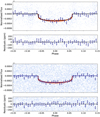 |
Fig. 1 Phase-folded light curve for planet b, over all of the (top) CHEOPS visits and (bottom) TESS sectors. Top subpanels: median fitted model (dark blue curves) and models computed from randomly drawn samples from the posterior (orange curves). The light blue and dark blue points are the original points and the binned data points. Bottom subpanels: residuals from the median model. |
2.3 Eclipse analysis
TOI-561 b orbits its host star at a short orbital distance of 0.0105 AU (see Table 2). We expect the dayside temperature2 of this planet to be around Tday ~ 2963.51 K for instant reradiation of the heat to the space (i.e. no heat redistribution) and Tday ~ 2319.07 K for a uniform heat distribution (effective temperature of the host star T★ = 5372 K; Lacedelli et al. 2022). Based on these estimates we expect the planet to produce strong thermal emission, even in the optical CHEOPS passband. In the light of previous CHEOPS measurements of planetary occultations (e.g. Lendl et al. 2020; Hooton et al. 2022), we thus search for a secondary eclipse signal in our dataset.
As our CHEOPS observations are focused on the transit event, most of the exposures do not cover the secondary eclipse of the planet. Fortunately though, two of the archival visits (Visit No. 39301 and 101, see Table 1) cover orbital phases during which occultation occurs five times. However, we found that these five occurrences are not enough to recover any significant signal from the CHEOPS data. Nonetheless, we derive a 99.7 percentile limit of 98.93 ppm on eclipse depth for this dataset.
On the other hand, TESS observed the event more than 150 times during its four observation sectors. Furthermore, we anticipated a larger occultation signal in the TESS data considering that the thermal contribution from TOI-561 b would be larger in the TESS bandpass than in the CHEOPS bandpass. With our upper estimation for the planet temperature Tday ~ 2963.51 K we expected the magnitude of the occultation to be at least 14 ppm in the TESS bandpass assuming black-body emission. To test this hypothesis, we modelled the TESS data with a joint transit-eclipse model and an only-transit model using batman models implemented in Juliet. We masked out the transit signals from all other planets to simplify the analysis. We used the same method as described in Sect. 2.2 to model the dataset, but this time we provided informative priors on all planetary parameters except the eclipse depth. We set a uniform prior between-100 ppm and 100 ppm for the eclipse depth. We compared the Bayesian evidence for a model comparison between the model with and without eclipse.
We find that the model with eclipse is strongly favoured statistically (Δ In Z ~ 1.43). The phase-folded light curve, including the median model with randomly selected models, is shown in Fig. 3. We were only able to put an upper limit on the eclipse depth (a 99.7 percentile limit of 60.15 ppm) because the value we derive from its posterior distribution (Fig. 3) is consistent with zero at 3σ:  ppm. The derived posterior can still put some constraints on the planetary atmosphere.
It should be noted here that both reflection and thermal emission could contribute to the occultation signal we are detecting in the TESS data. With TESS data alone we cannot determine the fractional contribution to the eclipse depth from these components, so that we would need similar observations at longer wavelengths. With the measured posterior of eclipse depth from the TESS data we can, however, estimate the geometric albedo (Ag) over a range of brightness temperatures (a measure of the thermal emission) for this planet. We followed the method from Mallonn et al. (2019) to find the relation between the geometric albedo and the temperature, which is plotted in Fig. 4. As expected, the median solution (orange line) is degenerate. The posterior of eclipse depth (as shown in Fig. 3, with  ppm), assuming a zero contribution from reflection, would result in a dayside temperature of ~3325 K. On the other hand, to explain the extracted eclipse depth with reflection alone, the geometric albedo of the planet should be around 0.83. We note that both of these values are the extreme cases, and that the true solution should lie somewhere in between.
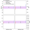 |
Fig. 2 Comparison of retrieved planetary parameters (P, a/R★, b, and Rp/R★) from our analyses of CHEOPS (blue points), TESS (red points), and the joint dataset (green points) with the literature values from Lacedelli et al. (2022; dashed purple line and a 1σ uncertainty band). The horizontal axis gives the arbitrary transit time. The scale on the vertical axis is relative and is centred on the literature value of the given parameter. |
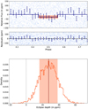 |
Fig. 3 Best-fit eclipse model to the TESS data along with the posteriors of the eclipse depth. Top panel, upper plot: median fitted model (dark blue curve), which includes the planet transit and eclipse, and the original (light blue) and binned data points (dark blue) from four TESS sectors. The orange curves are the models computed from the randomly chosen samples from the posteriors. The lower plot shows the residuals for the fit. Bottom panel: posterior distribution of the eclipse depth. The dark orange line and the light orange band give the median eclipse depth and the 1σ credible interval. The dashed line represents the null hypothesis. |
3 Internal structure modelling
In the following we discuss the internal structure of TOI-561 b. The method used is described in more depth in Leleu et al. (2021) and is based on Dorn et al. (2017), but we briefly summarise the most important aspects below. The Bayesian inference scheme we applied takes as input parameters the stellar observables (mass, radius, effective temperature, age, and [Si/H], [Mg/H], and [Fe/H]) and planetary observables (mass relative to the star, transit depth, and period) of the system. The likelihood of a given structure is calculated based on an internal structure model. We assume that the planet is spherically symmetric and consists of four fully distinct layers: an inner iron core (Hakim et al. 2018), a silicate mantle (Sotin et al. 2007), a water layer (Haldemann et al. 2020), and a pure H/He atmosphere (Lopez & Fortney 2014). Furthermore, we assume that the Si/Mg/Fe ratios of the planet match those of the star exactly. Although this is supported by Thiabaud et al. (2015), among others, recent work by Adibekyan et al. (2021) suggests that the correlation might not be 1:1. Implementing this possibility in the model is the subject of future work.
For the priors of the internal structure parameters, we chose a prior that is uniform in log for the gas mass. For the mass fractions of the inner core, mantle, and water layers with respect to the solid planet, our chosen prior is uniform with the added condition that they add up to one and with an upper limit of the water mass fraction of 50% (Thiabaud et al. 2014; Marboeuf et al. 2014). We note that the results of the internal structure modelling depend to a certain extent on the chosen priors.
We ran two different versions of our model for TOI-561 b. Given its high equilibrium temperature, any water layer would have evaporated and formed a thick water vapour atmosphere. However, with the current version of our model it is not possible to include such a critical steam layer. We therefore choose, on the one hand, to run a dry model of the planet without an added water layer. On the other hand, we also ran the full version of the model with an included water layer as this is the most general way to model the planet that our model allows, and any additional assumptions would in the end just be mirrored in the resulting posteriors. The resulting differences in the posteriors of the internal structure parameters are summarised in Table 3.
For the dry model, the posterior of the gas mass is quite well constrained with a median at around 10−7 M⊕. However, such a planet is unphysical as any H/He envelope would be evaporated very quickly. Figure 5 shows the resulting posterior distributions of the internal structure parameters of TOI-561 b when running the full version of the model. For both versions of the model, a planet that only consists of an iron core and a silicate mantle seems to be unlikely given the observations. The best model converges towards a water mass fraction that is constrained quite well, while the gas mass fraction is negligibly small, as expected from the strong irradiation of the planet. This finding and our core mass fraction is in agreement with a recent independent study that found a water- and gas-devoid planet can only reproduce the observed density with a composition much lower than the stellar value and the inclusion of a high melt fraction (Brinkman et al. 2023).
We note that in our model the inner layers of the planet are not influenced by the pressure or temperature of the atmosphere, which does have an influence on the modelled radius of the solid planet. To investigate the influence a higher temperature could have on the radius of the iron core and silicate mantle, we selected a subsample of points from our posterior distribution and used the forward model to recompute their radius when setting the temperature at the boundary between the atmosphere and the solid planet to the equilibrium temperature of TOI-561 b. This showed that raising the temperature of the iron core and the silicate mantle only results in an increase in radius of less than 3%, which is not enough to explain the difference in radius between the observations and a planet consisting only of an iron core and a silicate mantle.
Choosing different constraints for the Si/Mg/Fe ratios of the planet also influences the radius of the iron core and silicate mantle. As an extreme case, we used our forward model to calculate the thickness of these two layers for an iron-free planet, again with a temperature equal to the equilibrium temperature of TOI-561 b at the outer boundary. This gives a radius very close to that derived for TOI-561 b. Since a planet that is completely iron-free seems unlikely, we conclude that some heavier elements are in fact necessary. We also performed another Bayesian analysis where we lifted the compositional constraints on the planet by allowing the code to sample from a wide range of stellar abundances: ![Mathematical equation: $\left[ {{{{\rm{Si}}} \mathord{\left/ {\vphantom {{{\rm{Si}}} {\rm{H}}}} \right. \kern-\nulldelimiterspace} {\rm{H}}}} \right] = \left[ {{{{\rm{Mg}}} \mathord{\left/ {\vphantom {{{\rm{Mg}}} {\rm{H}}}} \right. \kern-\nulldelimiterspace} {\rm{H}}}} \right] = \left[ {{{{\rm{Fe}}} \mathord{\left/ {\vphantom {{{\rm{Fe}}} {\rm{H}}}} \right. \kern-\nulldelimiterspace} {\rm{H}}}} \right] = 0_{ - 1}^{ + 1}$](/articles/aa/full_html/2023/11/aa44946-22/aa44946-22-eq41.png) . The posteriors of the internal structure parameters resulting from this analysis are summarised in Table 4. For the Si/Fe and Mg/Fe ratios of the planet, the model gives posteriors of
. The posteriors of the internal structure parameters resulting from this analysis are summarised in Table 4. For the Si/Fe and Mg/Fe ratios of the planet, the model gives posteriors of  and
and  , while the corresponding ratios derived from the stellar abundances are
  and Mg/Fe = 2.02 ± 0.51. With this version of the model a pure iron-silicate structure also seems to be unlikely, given the observations.
However, this analysis still assumes the water layer to be in a condensed state and fully distinct from the H/He atmosphere. We therefore ran an additional exploratory internal structure analysis using a new version of our model that is fully self-consistent and features an H2O enriched envelope. More specifically, we assumed the planet to have an inner iron core and a silicate mantle with a fixed combined mass of 2.24 ± 0.20 M⊕ and a composition corresponding to the median of the posterior distribution obtained using the dry model without water layer described above. This assumption is justified since the gas mass we obtain when running a dry model is very low (see Table 3). We note that this new model version uses the atmosphere model of Parmentier & Guillot (2014) instead of the Lopez & Fortney (2014) model used in the remaining analysis. Then, we ran a grid of planetary forward models consisting of this fixed core and gas envelopes with different masses (going from mass fraction of 10−9 up to 10−6) and different envelope enrichments (with molar water fractions between 0 and 1). The results of this study can be seen in Fig. 6. For each grid point, the transit radius of the resulting structure is shown (in colour), with the red line depicting the measured radius of TOI-561 b. Any combination of envelope mass and enrichment Z that lies within the two other red lines is consistent with the measurements.
Posteriors of the internal structure parameters.
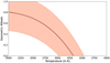 |
Fig. 4 Relation between geometric albedo and brightness temperature of the planet, given the posteriors of the occultation depth (with mean and 1σ intervals |

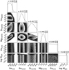 |
Fig. 5 Corner plot of the posteriors of the internal structure parameters of TOI-561 b. Shown are the mass fractions with respect to the solid planet of the inner core and water layer, the molar fractions of Si and Mg in the mantle layer and Fe in the inner core and the gas mass in Earth masses in a logarithmic scale. The labels at the top of each column are the median and the 5th and 95th percentiles of each distribution, which are also shown by the dashed lines. |
Posteriors of the internal structure parameters for models with fixed (to stellar values) and varying Si/MG/Fe ratios in the models.
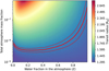 |
Fig. 6 Transit radius as a function of total envelope mass fraction and molar water fraction in the envelope for a planetary structure with a fixed core mass and composition in agreement with the values for a dry model in Table 3. The red lines show the radius values that are in agreement with the measurements for TOI-561 b. |
4 Prospects of an atmosphere
4.1 Interpreting the eclipse signal
The absence of thick (>0.1 bar) atmospheres on the inner two TRAPPIST-1 planets, as observed by JWST (Zieba et al. 2023; Greene et al. 2023), and even on a temperate rocky world like LHS 3844 b, as evidenced by Spitzer (Kreidberg et al. 2019), appears at a first glance to make the presence of an atmosphere on a USP like TOI-561 b even less likely.
Ultra-short-period planets, however, have such high surface temperatures (>2000 K) that their surfaces are expected to be at least partially molten, giving rise to tenuous evaporating atmospheres of more exotic compositions than on rocky planets in the Solar System. For example, a tenuous rock vapour atmosphere was suggested on K2-141b based on Kepler and Spitzer observations (Zieba et al. 2022). Thus, constraining evaporating atmospheres on USPs raised the tantalising prospect of assessing surface properties on rocky exoplanets more directly by observing spectral features of outgassed molecules (see e.g. Chao et al. 2021).
Recently, Zilinskas et al. (2022) put together an extensive catalogue of outgassed atmospheres for various USPs, including TOI-561 b, under different assumptions of surface composition and outgassing efficiency. These authors provided pressure temperature profiles for these different atmospheres that were calculated self-consistently, assuming irradiation at the substellar point without any heat distribution and assuming an albedo of 0. In the case of TOI-561 b, the model yields about 0.4 bar for 60% outgassing efficiency.
We used two planetary compositions, bulk silicate (oxidised) Earth (BSE) and evolved BSE (with 60% outgassing efficiency), to estimate the eclipse depth in the TESS bandpass to explain the measured eclipse signal described in Sect. 2.33. These two models yield SiO as the main volatile in the outgassed atmosphere. The predicted eclipse depths for these models are 27.81 ppm and 26.59 ppm, which is very close to the observed eclipse depth of 27.40 ppm. This points to the fact that the emission coming from the planet in the TESS bandpass is the result of thermal emission only. However, we note here that models assume zero albedo and no heat redistribution resulting in a hotter temperature profile (see e.g. Fig. 7a), which was already noted by Zilinskas et al. (2022) as a limitation of their methods. It has been pointed out, however, that lava surfaces should have very low albedos (Essack et al. 2020). Further, K2-141b, the only USP known to date with hints of an outgassed rock vapour atmospheres, exhibits a phase-curve consistent with a scenario without any heat redistribution.
Keeping in mind these caveats, we made predictions for potential CHEOPS and upcoming JWST observations of this planet. The BSE and evolved BSE models predict the eclipse depth of 18.74ppm and 17.18 ppm in the CHEOPS bandpass (orange and blue triangles in Fig. 7b). A larger observed depth in the CHEOPS bandpass could be a sign of a significant reflective component. However, it would take an impractically large number of observations (62 and 73 for two models) to constrain the above-mentioned eclipse depths at 3σ as the target is faint with G = 10.0 mag4. Furthermore, it is questionable whether lava worlds exhibit high albedos, at least if an oxidised silicate surface like that in the BSE scenario is assumed (Essack et al. 2020). It would take ultramafic surfaces composed of olivine and enstatite to assume larger albedos (>0.2; Hu et al. 2012).
On the other hand, the James Webb Space Telescope (JWST) would be ideal for observing the thermal emission from the planetary surface or its atmosphere. A Cycle 2 GO program (GO 3860, PI: J. Teske) aims to do the same by observing phase curves of the planet with NIRSpec/G395H. Here we use Zilinskas et al. (2022) models with PandExo (Batalha et al. 2017) to simulate observations for NIRSPec/G395H and MIRI/LRS. The NIRSpec/G395H instrument, which has a wavelength range of 2.87 – 5.18 µm, covers a SiO feature between 4 µm and 5 µm. With four occultations of the planet (as asked for in GO 3860) we can expect to detect this feature as a rise in eclipse depth after ~4 µm, as shown in upper left inset in Fig. 7b (orange and blue circles). Unfortunately, both BSE and evolved BSE models are very similar in this range. Therefore, the NIRSpec/G395H observations cannot distinguish between the two models. There is an additional SiO feature near ~9 µm covered by the MIRI/LRS wavelength range, 5.02–13.86 µm. This feature is interesting because the amplitude (along with the baseline) of the feature changes depending on the outgassing efficiency. As shown in Fig. 7b, the evolved BSE composition (in blue) has a lower amplitude and higher baseline of the feature compared to that of the BSE composition (in orange). Additionally, there is a small SiO2 feature near ~7 µm which is only present in the spectrum of the BSE composition (see the lower right inset in Fig. 7b). Both of these features can be helpful in distinguishing the two models. We note, however, that with the current precision of the MIRI/LRS instrument, it would be quite challenging to reach the required level of noise to differentiate between two models at higher statistical confidence. We used ten eclipse observations for our simulation here.
The white-light eclipse depth could be used to estimate the temperature of the planet and solve the degeneracy between thermal and reflective components (also shown in Fig. 4). As already mentioned, models from Zilinskas et al. (2022) suggest that the emission in the TESS bandpass only occurs because of thermal radiation. If this is the case, then the white-light eclipse depth should be around 121.9 and 123.7 ppm for NIRSpec/G395H and 154.7 and 154.8 ppm for MIRI/LRS, respectively for BSE and evolved BSE compositions (see Fig. 7b). A lower observed white-light eclipse depth in these bands would be a hint of lower dayside temperature and a non-zero bond albedo.
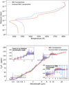 |
Fig. 7 Theoretical models of outgassed atmosphere of TOI-561 b. Top panel, a: Temperature-pressure profile of the planet for a bulk silicate Earth (BSE) composition (in orange) and an evolved BSE composition (in blue). Bottom panel, b: Theoretical emission spectra for BSE (orange curve) and evolved BSE (blue curve) composition. The TESS observation of the eclipse depth is shown as a green star, where the error bars on the wavelength axis show the extent of the TESS bandpass. Other data points are simulated observations for NIRSpec (circles), MIRI (squares), and CHEOPS (triangles) for both models (represented by the colours). The white-light eclipse depths are shown for NIRSpec and MIRI with errors showing their wavelength coverage. The two insets show the zoomed-in versions of the main plot for the NIRSpec and MIRI wavelength ranges. The spectroscopic simulated eclipse depths (at R = 7) are also shown for both instruments in these plots. |
4.2 Search for variability
As mentioned in Sect. 2.3, the dayside temperature of the planet can reach as high as ~3000 K, resulting in the surface of the planet being partially or completely molten. At this point the planet can support a secondary outgassed atmosphere made up of heavier species, such as Na, O2, and SiO. (Schaefer & Fegley 2009; Miguel et al. 2011; Schaefer et al. 2012; Wordsworth & Kreidberg 2022). Driven by winds, the species could travel to the nightside and condensate or even escape into space (Kite et al. 2016; Wordsworth & Kreidberg 2022). Both phenomena, influenced by the surface activity of the planet and the stellar irradiation, could lead to temporal variability in the atmospheric properties, which could potentially be imprinted on the Rp/R★ measured over several transit events.
Motivated by this rationale, we reanalysed all of the TESS and CHEOPS data, but now fixed all parameters except Rp /R★ to the values derived from our joint photometric analysis (Table 2). While for the CHEOPS data we model each transit individually, for TESS we group about five transit events together to achieve a better signal-to-noise ratio. The result of this analysis is presented in Fig. 8. It shows the difference in ppm between each measured Rp/R★ and the Rp/R★ from our joint analysis. As can be seen from Fig. 8, we find no significant variations in Rp/R★ over time. Although this does not rule out the possibility of the atmosphere being variable, our current dataset does not have the required precision.
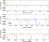 |
Fig. 8 Difference in ppm between the Rp/R★ measured in individual transits (for CHEOPS data) or groups of five transits (for TESS data), and the value of Rp/R★ from the joint CHEOPS-TESS analysis. The orange and blue points are the results from the TESS and CHEOPS analysis, respectively. |
5 Discussion and conclusions
Ultra-short-period planets are a singular class of planets that orbit their host star within a day. This property makes them appealing targets to study various compelling phenomena caused by the extreme proximity and radiation from the star, ranging from their internal structure to their atmospheres. Well-known USPs like 55 Cnce, K2-141 b, and LHS 3844 b display a diverse range of composition from a thick, possibly variable atmosphere to no atmosphere at all (Demory et al. 2016; Kreidberg et al. 2019; Zieba et al. 2022). Among the USP population, the newly discovered TOI-561 b stands apart for its unusually low density of  g cm−3 when other USPs show higher densities (see the position of TOI-561 b in the mass–radius diagram in Fig. 9).
To further place TOI-561 b in the context of known USPs and understand how the metal-poor nature of the host star may have affected its formation and evolution, we retrieved planet properties for all well-characterised bodies with an orbital period of less than a day and Mp ≤ 10 M⊕ from the NASA Exoplanet Archive (2023). To test how stellar composition may impact USPs, we first made the assumption that these bodies have entirely lost their primordial hydrogen atmosphere, and thus we were only observing the refractory components of the planets. To assess this assumption, we computed the minimum mean molecular weight (MMMW) of a potential atmosphere of our USP sample using a formulation of the Jeans escape criteria (Jeans 1925) that includes Roche lobe effects (Erkaev et al. 2007; Fossati et al. 2017) in a similar manner to Wilson et al. (2022). Given their current physical and orbital parameters, we find that all USPs, with the exception of TOI-1075b (Essack et al. 2023), cannot have held onto a primordial envelope, and thus that our assumption is valid. We recognise that other processes may have induced further atmospheric mass loss, and whilst the inclusion of this additional modelling is beyond the scope of this paper, any additional atmospheric escape would strengthen our assumption that USPs are primarily rocky. Furthermore, we find that the minimum mean molecular weight of an atmosphere that TOI-561 b can retain is 11 amu, providing evidence that the planet has likely lost its primordial atmosphere, but may have a heavier secondary envelope.
After making sure that the planets in our USP sample do not have primordial atmospheres, we assessed the physical properties of these well-characterised bodies to probe underlying processes. In the upper panel of Fig. 10 we plot the planetary surface gravity of rocky USPs, as determined by our MMMW analysis above, against their equilibrium temperature, which reveals a clear trend. To substantiate the identified correlation, we used a Bayesian correlation tool (Figueira et al. 2016) and find the median and standard deviation of the correlation metric distribution (similar to Spearman’s rank value) to be 0.45 ± 0.16. This strong trend is interpreted as lower surface gravity planets having lower gravitational potential wells that allow the escape of envelopes at lower temperatures, and hence appearing as the rocky USPs identified by our MMMW analysis. Adibekyan et al. (2021) have found evidence for stellar composition influencing planetary internal structure for terrestrial bodies. If this finding is universal, one would expect planets around metal-poor stars to have smaller iron cores, and thus lower surface gravities for bodies of a similar radius. Interestingly, if we remove metal-poor planets, [Fe/H] < −0.1, (TOI-561 b, Kepler-10b, Kepler-78b, and TOI-1685 b) from our USP sample, the correlation between surface gravity and equilibrium temperature increases to 0.65±0.13 because metal-poor USP planets have lower surface gravities at similar equilibrium temperatures. This supports previous findings that host star metallicity alters planet interior structure (Adibekyan et al. 2021; Wilson et al. 2022). This is highlighted in the lower panel of Fig. 10, where we removed the equilibrium temperature dependence by selecting USPs hotter than 1700 K and found a strong trend between surface gravity and host-star metallicity.
Figure 10 also clearly shows the uniqueness of TOI-561 b in temperature-metallicity-surface gravity space. All these factors motivated our follow-up of this planet with the state-of-the-art photometric telescope CHEOPS to precisely measure its radius, and therefore to constrain its composition and structure. We acquired 13 new transit observations of the planet with CHEOPS, and combined them with three archival visits from CHEOPS and four TESS sectors. This joint dataset allowed us to set strong constraints on the planet-to-star radius ratio, reducing its uncertainty to ~2%. We used our updated parameters for TOI-561 b to model its internal structure. We find that the structure of planet is consistent with a negligible primary volatile atmosphere made up of H/He, which is expected from the atmospheric escape from such a highly irradiated planet. Additionally, a planet built only from an iron core and silicate mantle is not enough to explain the observed density, which supports the presence of lighter material in the planetary structure. This could be a thin layer of high mean molecular weight (e.g. a water layer, as shown by our internal structure modelling), a larger silicate mantle than predicted using a one-to-one scaling between the stellar and planet composition, or a combination of both. We also ran a fully self-consistent exploratory forward model with a water enriched envelope and demonstrated that such a model can indeed explain the transit radius. We show that a range of water fraction in the atmosphere is possible for a varying atmospheric mass fraction. Given the high equilibrium temperature of the planet, a plausible scenario is that it sustains a secondary atmosphere containing heavy metal species. We searched for variations in Rp/R★ over time, which could trace the variability expected from such an envelope, but found no such evidence.
In addition to the transit observations, we also find a weak detection of the secondary eclipse in the TESS data, with an eclipse depth  ppm. Since this emission signal would be contaminated from the reflective and thermal radiation from the planet we cannot uniquely determine its geometric albedo and dayside temperature. The measured occultation depth would correspond to a dayside temperature of ~3325 K if the signal is assumed to originate entirely from thermal radiation; on the contrary, a 100% contribution from reflection would imply a geometric albedo of ~0.83. Given that the planet could possibly have a secondary metal-rich atmosphere, we used models of out-gassed atmospheres from Zilinskas et al. (2022) to explain this eclipse signal. The expected eclipse depths from the two model compositions, bulk silicate (oxidised) Earth (BSE) and evolved BSE composition with 60% outgassing efficiency, are 27.81 ppm and 26.59 ppm, which is very close to the observed value. This implies that the emission in TESS bandpass is mainly of thermal origin.
The composition of the atmosphere is essential in constraining the surface properties, given the possible atmosphere-interior interactions. Our photometric observations cannot constrain the presence of a specific species in the atmosphere of the planet. While ground-based spectroscopy could be used to search for light species escaping the planet, such as sodium or oxygen, space-based observations in the infrared could allow us to detect a mineral atmosphere. The recently launched James Webb Space Telescope (JWST) would be the ideal facility to search for dust and metals in the atmosphere of TOI-561 b, which is one of the main goals of the recently accepted Cycle 2 GO program (GO 3860, PI: J. Teske). Using the models from Zilinskas et al. (2022) we anticipate that these observations, which will use the NIRSpec/G395H instrument, should be able to detect SiO in the atmosphere. Observations in the mid-infrared using MIRI/LRS (a mode not used by GO 3860) could, in principle, not only detect the mineral species in the atmosphere, but also infer the surface evolution. Infrared observations have the other advantage of breaking the degeneracy between reflective and thermal contributions in the observed emission. Hence, with the help of observations at longer wavelengths, not only can we identify the composition of the atmosphere, we can also derive the temperature of the planet.
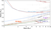 |
Fig. 9 Mass-radius diagram of exoplanets with Mp ≤ 10 M⊕ and Rp ≤ 4R⊕ known with a precision better than 30%. The grey points are all the known exoplanets as of June 19, 2023, taken from the NASA Exoplanet Archive (2023). The black dashed line is the iso-density curve for the value we derived for TOI-561 b. The mass of TOI-561 b is taken from Brinkman et al. (2023) and the radius from the present work. Also shown are the theoretical models for various chemical compositions computed by Zeng et al. (2019). The mass and radius of 55 Cnc e, K2-141 b, and CoRoT-7 b are taken from Bourrier et al. (2018), Malavolta et al. (2018), and John et al. (2022). |
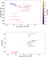 |
Fig. 10 Population of USPs in (top) planetary surface gravity– equilibrium temperature and (bottom) host star metallicity–surface gravity spaces. In the top panel the data points are colour-coded according to the metallicity of the host star. The USP population is defined as all confirmed planets with an orbital period of less than a day and Mp ≤ 10 M⊕. The data of the systems are taken from the NASA Exoplanet Archive (2023) on June 19, 2023. The bottom panel only includes planets hotter than 1700 K (see text). |
Acknowledgements
We would like to thank an anonymous referee for their detailed referee report and suggestions which significantly improved the manuscript. CHEOPS is an ESA mission in partnership with Switzerland with important contributions to the payload and the ground segment from Austria, Belgium, France, Germany, Hungary, Italy, Portugal, Spain, Sweden, and the United Kingdom. The CHEOPS Consortium would like to gratefully acknowledge the support received by all the agencies, offices, universities, and industries involved. Their flexibility and willingness to explore new approaches were essential to the success of this mission. This research has made use of the NASA Exoplanet Archive, which is operated by the California Institute of Technology, under contract with the National Aeronautics and Space Administration under the Exoplanet Exploration Program. J.A.P. would like to thank Yamila Miguel for an insightful discussion on the atmosphere of lava planets and for kindly providing theoretical models for our planet. J.A.P. and A.Br. were supported by the SNSA. J.A.E. and Y.A. acknowledge the support of the Swiss National Fund under grant 200020_172746. This project has received funding from the European Research Council (ERC) under the European Union’s Horizon 2020 research and innovation programme (project SPICE DUNE, grant agreement No 947634). A.C.C. and T.G.W. acknowledge support from STFC consolidated grant numbers ST/R000824/1 and ST/V000861/1, and UKSA grant number ST/R003203/1. L.Ca. acknowledges financial support from the Österreichische Akademie der Wissenschaften; L.Ca. acknowledges support from the European Union H2020-MSCA-ITN-2019 under Grant Agreement no. 860470 (CHAMELEON). S.G.S. acknowledges support from FCT through FCT contract nr. CEECIND/00826/2018 and POPH/FSE (EC). This project has received funding from the European Research Council (ERC) under the European Union’s Horizon 2020 research and innovation programme (project FOUR ACES; grant agreement No 724427). It has also been carried out in the frame of the National Centre for Competence in Research PlanetS supported by the Swiss National Science Foundation (SNSF). D.Eh. and A.De. acknowledge financial support from the SNSF for project 200021_200726. K.W.F.L. acknowledges support by DFG grants RA714/14-1 within the DFG Schwerpunkt SPP 1992, “Exploring the Diversity of Extrasolar Planets”. M.L. acknowledges support of the Swiss National Science Foundation under grant number PCEFP2_194576. We acknowledge support from the Spanish Ministry of Science and Innovation and the European Regional Development Fund through grants ESP2016-80435-C2-1-R, ESP2016-80435-C2-2-R, PGC2018-098153-B-C33, PGC2018-098153-B-C31, ESP2017-87676-C5-1-R, MDM-2017-0737 Unidad de Excelencia Maria de Maeztu-Centro de Astrobiología (INTA-CSIC), as well as the support of the Generalitat de Catalunya/CERCA programme. The MOC activities have been supported by the ESA contract No. 4000124370. S.C.C.B. acknowledges support from FCT through FCT contracts nr. IF/01312/2014/CP1215/CT0004. X.B., S.C., D.G., M.F. and J.L. acknowledge their role as ESA-appointed CHEOPS science team members. This project was supported by the CNES. The Belgian participation to CHEOPS has been supported by the Belgian Federal Science Policy Office (BELSPO) in the framework of the PRODEX Program, and by the University of Liège through an ARC grant for Concerted Research Actions financed by the Wallonia-Brussels Federation. L.D. is an F.R.S.-FNRS Postdoctoral Researcher. This work was supported by FCT - Fundação para a Ciência e a Tecnologia through national funds and by FEDER through COMPETE2020 - Programa Operacional Competitividade e Internacionalizacão by these grants: UID/FIS/04434/2019, UIDB/04434/2020, UIDP/04434/2020, PTDC/FIS-AST/32113/2017 & POCI-01-0145-FEDER-032113, PTDC/FIS-AST/28953/2017 & POCI-01-0145-FEDER-028953, PTDC/FIS-AST/28987/2017 & POCI-01-0145-FEDER-028987, O.D.S.D. is supported in the form of work contract (DL 57/2016/CP1364/CT0004) funded by national funds through FCT. B.-O.D. acknowledges support from the Swiss National Science Foundation (PP00P2-190080). M.F. gratefully acknowledges the support of the Swedish National Space Agency (DNR 65/19, 174/18). D.G. gratefully acknowledges financial support from the CRT foundation under Grant No. 2018.2323 “Gaseousor rocky? Unveiling the nature of small worlds”. M.G. is an F.R.S.-FNRS Senior Research Associate. S.H. gratefully acknowledges CNES funding through the grant 837319. K.G.I. is the ESA CHEOPS Project Scientist and is responsible for the ESA CHEOPS Guest Observers Programme. She does not participate in, or contribute to, the definition of the Guaranteed Time Programme of the CHEOPS mission through which observations described in this paper have been taken, nor to any aspect of target selection for the programme. This work was granted access to the HPC resources of MesoPSL financed by the Région Île de France and the project Equip@Meso (reference ANR-10-EQPX-29-01) of the programme Investissements d’Avenir supervised by the Agence Nationale pour la Recherche. P.M. acknowledges support from STFC research grant number ST/M001040/1. V.Na., I.Pa., G.Pi., R.Ra. and G.Sc. acknowledge support from CHEOPS ASI-INAF agreement n. 2019-29-HH.0. This work was also partially supported by a grant from the Simons Foundation (PI Queloz, grant number 327127). I.R.I. acknowledges support from the Spanish Ministry of Science and Innovation and the European Regional Development Fund through grant PGC2018-098153-B- C33, as well as the support of the Generalitat de Catalunya/CERCA programme. Gy.M.Sz. acknowledges the support of the Hungarian National Research, Development and Innovation Office (NKFIH) grant K-125015, a PRODEX Experiment Agreement No. 4000137122, the Lendület LP2018-7/2021 grant of the Hungarian Academy of Science and the support of the city of Szombathely. V.V.G. is an F.R.S-FNRS Research Associate. N.A.W. acknowledges UKSA grant ST/R004838/1.
Appendix A Photometric analysis without assuming prior knowledge of the stellar density
As mentioned in Section 2.2, in our joint transit fit for the full dataset of CHEOPS and TESS, we used informative priors on the stellar density. The stellar density adopted in the procedure was computed from the stellar mass and radius estimated from the stellar spectroscopic analysis performed in Lacedelli et al. (2022). For completeness, and to test the validity of our results, we performed another analysis. This time, we did not assume any prior knowledge of the stellar density. Therefore, in this analysis, we put wide uninformative priors on a/R★ (scaled semi-major axis, uniformally distributed priors in the log-space between 1 and 10) instead of using the stellar density. We illustrate the result of this analysis in Figure A.1 by comparing them with the analysis performed in Section 2.2.3. Given the precision and quantity of the data at hand, the planetary parameters agree very well with our analysis (with 3σ, even 1σ for some of them) when we use priors on the stellar density and with their literature counterparts from Lacedelli et al. (2022). However, as expected, the uncertainties on the parameters are increased in this analysis owing to our lack of knowledge of semi-major axis and/or stellar density.
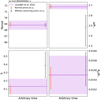 |
Fig. A.1 Comparison of some retrieved planetary parameters (Period P, scaled semi-major axis a/R★, impact parameter b, and planet-to-star radius ratio Rp/R★) between our two analyses. Shown are the main analysis, where we used informative priors on the stellar density (orange points), and the second analysis, where we assumed no prior knowledge on the stellar density (green points). The purple dashed line with the band shows the literature values of the parameters along with uncertainties from Lacedelli et al. (2022). The scale on the y-axis is relative. |
Appendix B Raw and detrended photometry from CHEOPS
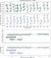 |
Fig. B.1 Raw and detrended CHEOPS observations. (a): Raw (top panel) and detrended photometry (bottom panel) for our new CHEOPS observations. The blue and orange points are the original and binned data points, respectively. The fitted median full model (top) and transit model (bottom) is shown as dark green lines. (b): Same as (a), but for archival CHEOPS visits. For clarity, the transit signals from other planets have been masked. |
Appendix C Correlation plot of the fitted transit parameters
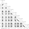 |
Fig. C.1 Correlation plot of the fitted transit parameters of planet b in our joint photometric analysis. |
References
- Adibekyan, V., Dorn, C., Sousa, S. G., et al. 2021, Science, 374, 330 [NASA ADS] [CrossRef] [Google Scholar]
- Asplund, M., Grevesse, N., Sauval, A. J., & Scott, P. 2009, ARA&A, 47, 481 [NASA ADS] [CrossRef] [Google Scholar]
- Batalha, N. E., Mandell, A., Pontoppidan, K., et al. 2017, PASP, 129, 064501 [Google Scholar]
- Beaugé, C., & Nesvorný, D. 2013, ApJ, 763, 12 [Google Scholar]
- Benz, W., Broeg, C., Fortier, A., et al. 2021, Exp. Astron., 51, 109 [Google Scholar]
- Borucki, W. J., Koch, D., Basri, G., et al. 2010, Science, 327, 977 [Google Scholar]
- Bourrier, V., Dumusque, X., Dorn, C., et al. 2018, A&A, 619, A1 [NASA ADS] [CrossRef] [EDP Sciences] [Google Scholar]
- Brinkman, C. L., Weiss, L. M., Dai, F., et al. 2023, AJ, 165, 88 [NASA ADS] [CrossRef] [Google Scholar]
- Brogi, M., Keller, C. U., de Juan Ovelar, M., et al. 2012, A&A, 545, L5 [NASA ADS] [CrossRef] [EDP Sciences] [Google Scholar]
- Burrows, A. S. 2014, PNAS, 111, 12601 [NASA ADS] [CrossRef] [Google Scholar]
- Chao, K.-H., de Graffenried, R., Lach, M., et al. 2021, Chemie der Erde/Geochemistry, 81, 125735 [NASA ADS] [Google Scholar]
- Chen, D.-C., Xie, J.-W., Zhou, J.-L., et al. 2022, AJ, 163, 249 [NASA ADS] [CrossRef] [Google Scholar]
- Davis, T. A., & Wheatley, P. J. 2009, MNRAS, 396, 1012 [CrossRef] [Google Scholar]
- Demory, B.-O., Gillon, M., Madhusudhan, N., & Queloz, D. 2016, MNRAS, 455, 2018 [NASA ADS] [CrossRef] [Google Scholar]
- Dorn, C., Venturini, J., Khan, A., et al. 2017, A&A, 597, A37 [NASA ADS] [CrossRef] [EDP Sciences] [Google Scholar]
- Ehrenreich, D., & Désert, J. M. 2011, A&A, 529, A136 [NASA ADS] [CrossRef] [EDP Sciences] [Google Scholar]
- Erkaev, N. V., Kulikov, Y. N., Lammer, H., et al. 2007, A&A, 472, 329 [NASA ADS] [CrossRef] [EDP Sciences] [Google Scholar]
- Espinoza, N., & Jordán, A. 2015, MNRAS, 450, 1879 [Google Scholar]
- Espinoza, N., Kossakowski, D., & Brahm, R. 2019, MNRAS, 490, 2262 [Google Scholar]
- Essack, Z., Seager, S., & Pajusalu, M. 2020, ApJ, 898, 160 [CrossRef] [Google Scholar]
- Essack, Z., Shporer, A., Burt, J. A., et al. 2023, AJ, 165, 47 [NASA ADS] [CrossRef] [Google Scholar]
- Figueira, P., Faria, J. P., Adibekyan, V. Z., Oshagh, M., & Santos, N. C. 2016, Orig. Life Evol. Biosph., 46, 385 [NASA ADS] [CrossRef] [Google Scholar]
- Foreman-Mackey, D. 2016, J. Open Source Softw., 1, 24 [Google Scholar]
- Foreman-Mackey, D., Agol, E., Ambikasaran, S., & Angus, R. 2017, AJ, 154, 220 [Google Scholar]
- Fossati, L., Erkaev, N. V., Lammer, H., et al. 2017, A&A, 598, A90 [NASA ADS] [CrossRef] [EDP Sciences] [Google Scholar]
- Greene, T. P., Bell, T. J., Ducrot, E., et al. 2023, Nature, 618, 39 [NASA ADS] [CrossRef] [Google Scholar]
- Hakim, K., Rivoldini, A., Van Hoolst, T., et al. 2018, Icarus, 313, 61 [Google Scholar]
- Haldemann, J., Alibert, Y., Mordasini, C., & Benz, W. 2020, A&A, 643, A105 [NASA ADS] [CrossRef] [EDP Sciences] [Google Scholar]
- Higson, E., Handley, W., Hobson, M., & Lasenby, A. 2019, Stat. Comput., 29, 891 [Google Scholar]
- Hooton, M. J., Hoyer, S., Kitzmann, D., et al. 2022, A&A, 658, A75 [NASA ADS] [CrossRef] [EDP Sciences] [Google Scholar]
- Howell, S. B., Sobeck, C., Haas, M., et al. 2014, PASP, 126, 398 [Google Scholar]
- Hoyer, S., Guterman, P., Demangeon, O., et al. 2020, A&A, 635, A24 [NASA ADS] [CrossRef] [EDP Sciences] [Google Scholar]
- Hu, R., Ehlmann, B. L., & Seager, S. 2012, ApJ, 752, 7 [NASA ADS] [CrossRef] [Google Scholar]
- Jeans, J. 1925, The Dynamical Theory of Gases (Cambridge University Press) [Google Scholar]
- Jenkins, J. M., Twicken, J. D., McCauliff, S., et al. 2016, in Society of Photo-Optical Instrumentation Engineers (SPIE) Conference Series, 9913, Software and Cyberinfrastructure for Astronomy IV, eds. G. Chiozzi, & J. C. Guzman, 99133E [Google Scholar]
- John, A. A., Collier Cameron, A., & Wilson, T. G. 2022, MNRAS, 515, 3975 [Google Scholar]
- Kipping, D. M. 2013, MNRAS, 435, 2152 [Google Scholar]
- Kite, E. S., Fegley, Bruce, J., Schaefer, L., & Gaidos, E. 2016, ApJ, 828, 80 [NASA ADS] [CrossRef] [Google Scholar]
- Koll, D. D. B., Malik, M., Mansfield, M., et al. 2019, ApJ, 886, 140 [NASA ADS] [CrossRef] [Google Scholar]
- Kreidberg, L. 2015, PASP, 127, 1161 [Google Scholar]
- Kreidberg, L., Koll, D. D. B., Morley, C., et al. 2019, Nature, 573, 87 [NASA ADS] [CrossRef] [Google Scholar]
- Lacedelli, G., Malavolta, L., Borsato, L., et al. 2021, MNRAS, 501, 4148 [NASA ADS] [CrossRef] [Google Scholar]
- Lacedelli, G., Wilson, T. G., Malavolta, L., et al. 2022, MNRAS, 511, 4551 [NASA ADS] [CrossRef] [Google Scholar]
- Lecavelier des Etangs, A. 2007, A&A, 461, 1185 [NASA ADS] [CrossRef] [EDP Sciences] [Google Scholar]
- Lecavelier des Etangs, A., Vidal-Madjar, A., McConnell, J. C., & Hébrard, G. 2004, A&A, 418, L1 [NASA ADS] [CrossRef] [EDP Sciences] [Google Scholar]
- Léger, A., Grasset, O., Fegley, B., et al. 2011, Icarus, 213, 1 [CrossRef] [Google Scholar]
- Leleu, A., Alibert, Y., Hara, N. C., et al. 2021, A&A, 649, A26 [NASA ADS] [CrossRef] [EDP Sciences] [Google Scholar]
- Lendl, M., Csizmadia, S., Deline, A., et al. 2020, A&A, 643, A94 [EDP Sciences] [Google Scholar]
- Lopez, E. D., & Fortney, J. J. 2013, ApJ, 776, 2 [Google Scholar]
- Lopez, E. D., & Fortney, J. J. 2014, ApJ, 792, 1 [Google Scholar]
- Lundkvist, M. S., Kjeldsen, H., Albrecht, S., et al. 2016, Nat. Commun., 7, 11201 [Google Scholar]
- Malavolta, L., Mayo, A. W., Louden, T., et al. 2018, AJ, 155, 107 [NASA ADS] [CrossRef] [Google Scholar]
- Mallonn, M., Köhler, J., Alexoudi, X., et al. 2019, A&A, 624, A62 [NASA ADS] [CrossRef] [EDP Sciences] [Google Scholar]
- Marboeuf, U., Thiabaud, A., Alibert, Y., Cabral, N., & Benz, W. 2014, A&A, 570, A36 [NASA ADS] [CrossRef] [EDP Sciences] [Google Scholar]
- Maxted, P. F. L., Ehrenreich, D., Wilson, T. G., et al. 2022, MNRAS, 514, 77 [NASA ADS] [CrossRef] [Google Scholar]
- Miguel, Y., Kaltenegger, L., Fegley, B., & Schaefer, L. 2011, ApJ, 742, L19 [NASA ADS] [CrossRef] [Google Scholar]
- Morris, B. M., Delrez, L., Brandeker, A., et al. 2021, A&A, 653, A173 [NASA ADS] [CrossRef] [EDP Sciences] [Google Scholar]
- NASA Exoplanet Archive 2023, Planetary Systems Composite Parameters, IPAC, https://catcopy.ipac.caltech.edu/dois/doi.php?id=10.26133/NEA13 [Google Scholar]
- Owen, J. E. 2019, Annu. Rev. Earth Planet. Sci., 47, 67 [CrossRef] [Google Scholar]
- Owen, J. E., & Jackson, A. P. 2012, MNRAS, 425, 2931 [Google Scholar]
- Owen, J. E., & Wu, Y. 2013, ApJ, 775, 105 [Google Scholar]
- Owen, J. E., & Wu, Y. 2016, ApJ, 817, 107 [NASA ADS] [CrossRef] [Google Scholar]
- Parmentier, V., & Guillot, T. 2014, A&A, 562, A133 [NASA ADS] [CrossRef] [EDP Sciences] [Google Scholar]
- Patel, J. A., & Espinoza, N. 2022, AJ, 163, 228 [NASA ADS] [CrossRef] [Google Scholar]
- Rappaport, S., Levine, A., Chiang, E., et al. 2012, ApJ, 752, 1 [NASA ADS] [CrossRef] [Google Scholar]
- Rappaport, S., Barclay, T., DeVore, J., et al. 2014, ApJ, 784, 40 [NASA ADS] [CrossRef] [Google Scholar]
- Raymond, S. N., Barnes, R., & Mandell, A. M. 2008, MNRAS, 384, 663 [Google Scholar]
- Ricker, G. R., Winn, J. N., Vanderspek, R., et al. 2014, in Society of Photo-Optical Instrumentation Engineers (SPIE) Conference Series, 9143, Space Telescopes and Instrumentation 2014: Optical, Infrared, and Millimeter Wave, eds. J. Oschmann, Jacobus, M., M. Clampin, G. G. Fazio, & H. A. MacEwen, 914320 [Google Scholar]
- Schaefer, L., & Fegley, B. 2009, ApJ, 703, L113 [CrossRef] [Google Scholar]
- Schaefer, L., Lodders, K., & Fegley, B. 2012, ApJ, 755, 41 [NASA ADS] [CrossRef] [Google Scholar]
- Skilling, J. 2004, in AIP Conf. Ser., 735, Bayesian Inference and Maximum Entropy Methods in Science and Engineering: 24th International Workshop on Bayesian Inference and Maximum Entropy Methods in Science and Engineering, eds. R. Fischer, R. Preuss, & U. V. Toussaint, 395 [NASA ADS] [CrossRef] [Google Scholar]
- Skilling, J. 2006, Bayesian Anal., 1, 833 [Google Scholar]
- Smith, J. C., Stumpe, M. C., Van Cleve, J. E., et al. 2012, PASP, 124, 1000 [Google Scholar]
- Sotin, C., Grasset, O., & Mocquet, A. 2007, Icarus, 191, 337 [Google Scholar]
- Speagle, J. S. 2020, MNRAS, 493, 3132 [Google Scholar]
- Stumpe, M. C., Smith, J. C., Catanzarite, J. H., et al. 2014, PASP, 126, 100 [Google Scholar]
- Szabó, G. M., & Kiss, L. L. 2011, ApJ, 727, L44 [Google Scholar]
- Szabó, G. M., Gandolfi, D., Brandeker, A., et al. 2021, A&A, 654, A159 [NASA ADS] [CrossRef] [EDP Sciences] [Google Scholar]
- Thiabaud, A., Marboeuf, U., Alibert, Y., et al. 2014, A&A, 562, A27 [NASA ADS] [CrossRef] [EDP Sciences] [Google Scholar]
- Thiabaud, A., Marboeuf, U., Alibert, Y., Leya, I., & Mezger, K. 2015, A&A, 574, A138 [NASA ADS] [CrossRef] [EDP Sciences] [Google Scholar]
- Venturini, J., Guilera, O. M., Ronco, M. P., & Mordasini, C. 2020, A&A, 644, A174 [NASA ADS] [CrossRef] [EDP Sciences] [Google Scholar]
- Weiss, L. M., Dai, F., Huber, D., et al. 2021, AJ, 161, 56 [NASA ADS] [CrossRef] [Google Scholar]
- Wilson, T. G., Goffo, E., Alibert, Y., et al. 2022, MNRAS, 511, 1043 [NASA ADS] [CrossRef] [Google Scholar]
- Winn, J. N., Sanchis-Ojeda, R., Rogers, L., et al. 2017, AJ, 154, 60 [NASA ADS] [CrossRef] [Google Scholar]
- Winn, J. N., Sanchis-Ojeda, R., & Rappaport, S. 2018, New A Rev., 83, 37 [Google Scholar]
- Wordsworth, R., & Kreidberg, L. 2022, ARA&A, 60, 159 [NASA ADS] [CrossRef] [Google Scholar]
- Zeng, L., Jacobsen, S. B., Sasselov, D. D., et al. 2019, PNAS, 116, 9723 [Google Scholar]
- Zieba, S., Zilinskas, M., Kreidberg, L., et al. 2022, A&A, 664, A79 [NASA ADS] [CrossRef] [EDP Sciences] [Google Scholar]
- Zieba, S., Kreidberg, L., Ducrot, E., et al. 2023, Nature, 620, 746 [NASA ADS] [CrossRef] [Google Scholar]
- Zilinskas, M., van Buchem, C. P. A., Miguel, Y., et al. 2022, A&A, 661, A126 [NASA ADS] [CrossRef] [EDP Sciences] [Google Scholar]
Calculated using  with the bond albedo AB = 0, and the heat redistribution factor f = 2/3 for a bare rock with no heat redistribution and f = 1/4 for uniform heat distribution (Burrows 2014; Koll et al. 2019).
Models are publicly available at https://github.com/zmantas/LavaPlanets
We used CHEOPS Exposure Time Calculator (https://cheops.unige.ch/pht2/exposure-time-calculator/) to estimate this.
All Tables
Posteriors of the internal structure parameters for models with fixed (to stellar values) and varying Si/MG/Fe ratios in the models.
All Figures
|
Fig. 1 Phase-folded light curve for planet b, over all of the (top) CHEOPS visits and (bottom) TESS sectors. Top subpanels: median fitted model (dark blue curves) and models computed from randomly drawn samples from the posterior (orange curves). The light blue and dark blue points are the original points and the binned data points. Bottom subpanels: residuals from the median model. |
| In the text | |
|
Fig. 2 Comparison of retrieved planetary parameters (P, a/R★, b, and Rp/R★) from our analyses of CHEOPS (blue points), TESS (red points), and the joint dataset (green points) with the literature values from Lacedelli et al. (2022; dashed purple line and a 1σ uncertainty band). The horizontal axis gives the arbitrary transit time. The scale on the vertical axis is relative and is centred on the literature value of the given parameter. |
| In the text | |
|
Fig. 3 Best-fit eclipse model to the TESS data along with the posteriors of the eclipse depth. Top panel, upper plot: median fitted model (dark blue curve), which includes the planet transit and eclipse, and the original (light blue) and binned data points (dark blue) from four TESS sectors. The orange curves are the models computed from the randomly chosen samples from the posteriors. The lower plot shows the residuals for the fit. Bottom panel: posterior distribution of the eclipse depth. The dark orange line and the light orange band give the median eclipse depth and the 1σ credible interval. The dashed line represents the null hypothesis. |
| In the text | |
|
Fig. 4 Relation between geometric albedo and brightness temperature of the planet, given the posteriors of the occultation depth (with mean and 1σ intervals |
| In the text | |
|
Fig. 5 Corner plot of the posteriors of the internal structure parameters of TOI-561 b. Shown are the mass fractions with respect to the solid planet of the inner core and water layer, the molar fractions of Si and Mg in the mantle layer and Fe in the inner core and the gas mass in Earth masses in a logarithmic scale. The labels at the top of each column are the median and the 5th and 95th percentiles of each distribution, which are also shown by the dashed lines. |
| In the text | |
|
Fig. 6 Transit radius as a function of total envelope mass fraction and molar water fraction in the envelope for a planetary structure with a fixed core mass and composition in agreement with the values for a dry model in Table 3. The red lines show the radius values that are in agreement with the measurements for TOI-561 b. |
| In the text | |
|
Fig. 7 Theoretical models of outgassed atmosphere of TOI-561 b. Top panel, a: Temperature-pressure profile of the planet for a bulk silicate Earth (BSE) composition (in orange) and an evolved BSE composition (in blue). Bottom panel, b: Theoretical emission spectra for BSE (orange curve) and evolved BSE (blue curve) composition. The TESS observation of the eclipse depth is shown as a green star, where the error bars on the wavelength axis show the extent of the TESS bandpass. Other data points are simulated observations for NIRSpec (circles), MIRI (squares), and CHEOPS (triangles) for both models (represented by the colours). The white-light eclipse depths are shown for NIRSpec and MIRI with errors showing their wavelength coverage. The two insets show the zoomed-in versions of the main plot for the NIRSpec and MIRI wavelength ranges. The spectroscopic simulated eclipse depths (at R = 7) are also shown for both instruments in these plots. |
| In the text | |
|
Fig. 8 Difference in ppm between the Rp/R★ measured in individual transits (for CHEOPS data) or groups of five transits (for TESS data), and the value of Rp/R★ from the joint CHEOPS-TESS analysis. The orange and blue points are the results from the TESS and CHEOPS analysis, respectively. |
| In the text | |
|
Fig. 9 Mass-radius diagram of exoplanets with Mp ≤ 10 M⊕ and Rp ≤ 4R⊕ known with a precision better than 30%. The grey points are all the known exoplanets as of June 19, 2023, taken from the NASA Exoplanet Archive (2023). The black dashed line is the iso-density curve for the value we derived for TOI-561 b. The mass of TOI-561 b is taken from Brinkman et al. (2023) and the radius from the present work. Also shown are the theoretical models for various chemical compositions computed by Zeng et al. (2019). The mass and radius of 55 Cnc e, K2-141 b, and CoRoT-7 b are taken from Bourrier et al. (2018), Malavolta et al. (2018), and John et al. (2022). |
| In the text | |
|
Fig. 10 Population of USPs in (top) planetary surface gravity– equilibrium temperature and (bottom) host star metallicity–surface gravity spaces. In the top panel the data points are colour-coded according to the metallicity of the host star. The USP population is defined as all confirmed planets with an orbital period of less than a day and Mp ≤ 10 M⊕. The data of the systems are taken from the NASA Exoplanet Archive (2023) on June 19, 2023. The bottom panel only includes planets hotter than 1700 K (see text). |
| In the text | |
|
Fig. A.1 Comparison of some retrieved planetary parameters (Period P, scaled semi-major axis a/R★, impact parameter b, and planet-to-star radius ratio Rp/R★) between our two analyses. Shown are the main analysis, where we used informative priors on the stellar density (orange points), and the second analysis, where we assumed no prior knowledge on the stellar density (green points). The purple dashed line with the band shows the literature values of the parameters along with uncertainties from Lacedelli et al. (2022). The scale on the y-axis is relative. |
| In the text | |
|
Fig. B.1 Raw and detrended CHEOPS observations. (a): Raw (top panel) and detrended photometry (bottom panel) for our new CHEOPS observations. The blue and orange points are the original and binned data points, respectively. The fitted median full model (top) and transit model (bottom) is shown as dark green lines. (b): Same as (a), but for archival CHEOPS visits. For clarity, the transit signals from other planets have been masked. |
| In the text | |
|
Fig. C.1 Correlation plot of the fitted transit parameters of planet b in our joint photometric analysis. |
| In the text | |
Current usage metrics show cumulative count of Article Views (full-text article views including HTML views, PDF and ePub downloads, according to the available data) and Abstracts Views on Vision4Press platform.
Data correspond to usage on the plateform after 2015. The current usage metrics is available 48-96 hours after online publication and is updated daily on week days.
Initial download of the metrics may take a while.