| Issue |
A&A
Volume 664, August 2022
|
|
|---|---|---|
| Article Number | A129 | |
| Number of page(s) | 22 | |
| Section | Numerical methods and codes | |
| DOI | https://doi.org/10.1051/0004-6361/202142402 | |
| Published online | 18 August 2022 | |
J-PLUS: Detecting and studying extragalactic globular clusters
The case of NGC 1023★
1
Núcleo de Astronomía, Universidad Diego Portales,
Ejército 441,
Santiago, Chile
e-mail: This email address is being protected from spambots. You need JavaScript enabled to view it.
2
Universidade de São Paulo, Instituto de Astronomia, Geofísica e Ciências Atmosféricas,
R. do Matão 1226,
São Paulo, SP
05508-090, Brazil
3
Observatório do Valongo, Universidade Federal do Rio de Janeiro,
Ladeira do Pedro Antônio 43,
Rio de Janeiro, RJ
20080-090, Brazil
4
Instituto de Radioastronomía y Astrofísica, Universidad Nacional Autónoma de México,
Morelia, Michoacán
58089, Mexico
5
Centro de Investigaciones de Astronomía (CIDA),
Mérida
5101, Venezuela
6
Instituto de Física, Universidade Federal do Rio Grande do Sul,
Av. Bento Gonçalves 9500,
Porto Alegre, R.S.
90040-060, Brazil
7
Shanghai Astronomical Observatory, Chinese Academy of Sciences,
80 Nandan Road,
Shanghai
200030, PR China
8
Universidade do Vale do Paraíba,
Av. Shishima Hifumi, 2911,
São José dos Campos, SP
12244-000, Brazil
9
Centro de Estudios de Física del Cosmos de Aragón, Unidad Asociada al CSIC,
Plaza San Juan 1,
44001
Teruel, Spain
10
Centre for Astrophysics & Supercomputing, Swinburne University,
Hawthorn VIC
3122, Australia
11
Instituto de Astrofísica de Andalucía – CSIC,
Glorieta de la Astronomía s/n,
18008
Granada, Spain
12
Instituto de Astrofísica de Canarias,
Calle Vía Láctea SN,
ES38205
La Laguna, Spain
13
Departamento de Astrofísica, Universidad de La Laguna,
ES38205
La Laguna, Spain
14
Observatório Nacional – MCTI (ON),
Rua Gal. José Cristino 77, São Cristóvão,
20921-400
Rio de Janeiro, Brazil
15
Ikerbasque, Basque Foundation for Science,
48013
Bilbao, Spain
Received:
8
October
2021
Accepted:
6
May
2022
Abstract
Context. Extragalactic globular clusters (GCs) are key objects in studies of galactic histories. The advent of wide-field surveys, such as the Javalambre Photometric Local Universe Survey (J-PLUS), offers new possibilities for the study of these systems.
Aims. We performed the first study of GCs in J-PLUS to recover information on the history of NGC 1023, taking advantage of wide-field images and 12 filters.
Methods. We developed the semiautomatic pipeline GCFinder for detecting GC candidates in J-PLUS images, which can also be adapted to similar surveys. We studied the stellar population properties of a sub-sample of GC candidates using spectral energy distribution (SED) fitting.
Results. We found 523 GC candidates in NGC 1023, about 300 of which are new. We identified subpopulations of GC candidates, where age and metallicity distributions have multiple peaks. By comparing our results with the simulations, we report a possible broad age-metallicity relation, supporting the notion that NGC 1023 has experienced accretion events in the past. With a dominating age peak at 1010 yr, we report a correlation between masses and ages that suggests that massive GC candidates are more likely to survive the turbulent history of the host galaxy. Modeling the light of NGC 1023, we find two spiral-like arms and detect a displacement of the galaxy’s photometric center with respect to the outer isophotes and center of GC distribution (~700pc and ~1600pc, respectively), which could be the result of ongoing interactions between NGC 1023 and NGC 1023A.
Conclusions. By studying the GC system of NGC 1023 with J-PLUS, we showcase the power of multi-band surveys for these kinds of studies and we find evidence to support the complex accretion history of the host galaxy.
Key words: galaxies: star clusters: general / galaxies: individual: NGC 1023 / surveys
A table containing the GC candidates presented in this work as well as their magnitudes is only available at the CDS via anonymous ftp to cdsarc.u-strasbg.fr (130.79.128.5) or via http://cdsarc.u-strasbg.fr/viz-bin/cat/J/A+A/664/A129
© D. de Brito Silva et al. 2022
 Open Access article, published by EDP Sciences, under the terms of the Creative Commons Attribution License (https://creativecommons.org/licenses/by/4.0), which permits unrestricted use, distribution, and reproduction in any medium, provided the original work is properly cited.
This article is published in open access under the Subscribe-to-Open model. This email address is being protected from spambots. You need JavaScript enabled to view it. to support open access publication.
1 Introduction
Globular clusters (GCs) are ubiquitous compact stellar systems found in most galaxies with stellar masses Mstar > 1068 M⊙ (e.g., Eadie et al. 2022). Some of these objects are among the oldest in the universe (Larsen 2001), with typical ages larger than 10Gyr (Strader et al. 2005; Chies-Santos et al. 2011). The investigation of GCs can shed light on how galaxies form and evolve through time, since these objects can be used to study galaxy assembly, star formation history, and their galaxy’s chemical evolution, among other aspects (Brodie & Strader 2006; Beasley 2020). As discussed in Brodie & Strader (2006), the typical mass of GCs is between 104 and 106 M⊙ and the size of the GC population in a galaxy is a function of galaxy luminosity, ranging from zero to a few in dwarf galaxies all the way up to more than 10 000 in cD galaxies (Alamo-Martínez & Blakeslee 2017).
A well-described property of the globular cluster population of a massive galaxy is its optical color bimodality, showing that there are subpopulations of this class of objects in most massive galaxies (Peng et al. 2006). The bimodality in GC colors is believed to occur due to differences in metallicities. However, age effects and a combination of age and metallicities effects might also play a vital role (Brodie & Strader 2006; Lee et al. 2018). It might also be important to take into account non-linear effects in the color-metallicity relations brought by the horizontal-branch morphology in the optical bands (Richtler 2005; Yoon et al. 2006, 2011; Cantiello & Blakeslee 2007; Chung et al. 2016; Lee et al. 2018, Lee et al. 2020; Villaume et al. 2019; Kim et al. 2021). Spectroscopic studies have shown that the blue subpopulations of GCs are more metal-poor than the red populations (Beasley et al. 2008; Usher et al. 2012). From chemical evolution models of galaxies as well as from observations, it is known that in dwarf irregular galaxies and low-mass galaxies, there is a tendency for GCs to be metal-poor and blue (Lotz et al. 2004). The fact that most galaxies tend to have sub-populations of GCs can be explained by a hierarchical formation: to form a massive system, many small systems are merged throughout time. We note that the optical/NIR colors of GC candidates do not have such bimodal distributions in most galaxies, except for NGC 3115, which appears to be bimodal (Brodie et al. 2012; Cantiello et al. 2014) in any color and metallicity studied (see Cantiello & Blakeslee 2007; Blakeslee et al. 2012; Cantiello et al. 2014; Cho et al. 2016).
Considering the extent to which the colors, ages, and metallicities of GCs are important in understanding the assembly of galaxies and their evolution, investigations of new photometric bands and colors as well as the interactions of new colors with stellar models and libraries can be interesting in terms of building more detailed spectral energy distributions (SEDs) for these systems. The Javalambre Photometric Local Universe Survey1 (J-PLUS; Cenarro et al. 2019) operates with a set of five broadband filters based on SDSS (York et al. 2000; Strauss et al. 2002) and seven narrowband filters that cover the main stellar indices from 370 to 900 nm ([OII], Ca H+K, D4000, Hδ, Mgb, Hα, and CaT). This filter set makes it possible to study GCs with novel colors and more detailed SEDs. Other surveys that can also add new colors to the study of extragalactic GCs are J-PAS (Javalambre Physics of the Accelerating Universe Astrophysical Survey; Benitez et al. 2014) and S-PLUS (Southern Photometric Local Universe Survey; Mendes de Oliveira et al. 2019). J-PAS is composed of 56 narrow–band filters in the optical, while S-PLUS has similar properties to J-PLUS, employing a twin filter system.
To explore the J-PLUS filter set in studies of extragalactic GCs, we take the SB0 galaxy NGC 1023 as a test case. NGC 1023 located at 11.1 Mpc away from Earth (Brodie et al. 2014), with an effective radius of 48″ (Dolfi et al. 2021). This galaxy is located at the center of a small group of galaxies (Tully 1980) and it is currently undergoing a minor merger with NGC 1023 A (Barbon & Capaccioli 1975; Hart et al. 1980; Capaccioli et al. 1986). NGC 1023 is characterized by a complex and extended HI cloud, whose densest clump is associated with the companion galaxy (Sancisi et al. 1984; Morganti et al. 2006). The characteristics of NGC 1023 are consistent with it being composed of a nearly classical bulge and a fast-rotating disk, as extracted from its planetary nebulae system (Noordermeer et al. 2008; Cortesi et al. 2011). Its star cluster system has been explored previously in the literature, including spectroscopic studies (e.g., Larsen 2001; Chies-Santos et al. 2013; Forbes et al. 2014) and it presents complex kinematics that are characterized by rotation in the inner disk-dominated region and gradually turning into a pressure-supported system in the outer halo-dominated part (Cortesi et al. 2016). The photometric studies trace the GC system up to eight effective radii (Kartha et al. 2014) and the spectroscopic sample is selected from the photometric sample to maximize the construction of multi-object spectroscopy (MOS) masks, leading to a non-uniform catalog of GCs ages, metallicities, and velocities.
NGC 1023 was observed with the Javalambre Auxiliary Survey Telescope (JAST80). The data were obtained with a Director’s Discretionary Time (DDT) proposal observed during science verification. The globular cluster luminosity function (GCLF) peak is at MV = −7.5 (Harris 2001), which corresponds to V ≈ 22.7 at 11.1 Mpc. J-PLUS reaches g = 21.5 with a signal-to-noise ratio (S/N) of 5 (Cenarro et al. 2019), which allows us to study the brightest part of the GCLF at these distances. On the other hand, the observations of NGC 1023 used in this article were not carried out with the standard exposure times of J-PLUS and so, we are also able to detect faint objects. In particular, we detected about 50% of expected objects with magnitudes between the peak of GCLF and 1 sigma below it, and with no objects between 2 and 3 sigmas below the peak of GCLF. As a result, our sample represents the majority of GC candidates expected for NGC 1023.
In this work, we propose a methodology for detecting and selecting GC candidates from images obtained with JAST80, aimed at exploiting data from J-PLUS that can be easily adapted for other photometric surveys such as J-PAS and S-PLUS (see also Buzzo et al. 2022 and Chies-Santos et al. 2022). With a catalog of GCs, we are set to investigate the stellar population content of GC candidates in NGC 1023 to create an unbiased magnitude limited catalog. This fact makes this galaxy an excellent case of study as we can explore new methodologies and colors, as well as to compare these results to other findings in the literature.
In Sect. 2, we describe the data used in this article. In Sect. 3, we present our methodology for detecting and selecting GC candidates, as well as our pipeline GCFinder. In Sect. 4, we present our results. In Sect. 5, we discuss our findings. Finally, in Sect. 6, we give our conclusions.
2 Data
NGC 1023 was observed in July 2017 through the DDT proposal 1600101 (P.I.: Ana Chies Santos) using JAST80 and T80Cam, a the panoramic camera of 9.2k × 9.2k pixels that provides a 2 deg2 field of view (FoV) with a pixel scale of 0.55 arcsec pix−1 (Marín-Franch et al. 2015).
These data are not part of J-PLUS, but they were observed as part of the commissioning period to test the survey capabilities for extragalactic GC science. This galaxy was observed using all filters available at the JAST80 telescope, namely the broadbands u, g, r, i, z as well as the narrowbands J0378, J0395, J0410, J0430, J0515, J0660, J0861. However, due to problems related to the calibration of the image referring to the J0395 band, we do not use this band in our work. The data are publicly available2. The full width at half maximum (FWHM) is presented in Table 1, as well as the exposure times. A color image of NGC 1023 is presented in Fig. 1, built using the software Trilogy (Coe et al. 2012).
To perform this study we started by cropping the original wide-field images to a smaller region of approximately 2000 X 1500 pixels (≈0.1 deg2) around NGC 1023 using IRAF (Tody 1993) tasks. The images have been reduced with the standard pipeline developed by the Data Processing and Archiving Unit (Unidad de Procesado y Archivo de Datos; hereafter UPAD) of CEFCA. In short, the process includes a correction for bias, flat-field, fringing, handling contaminants (cosmic rays, satellite traces, calibrating astrometry, and combining individual images of the same region into deeper images (for further details see Sect. 2.5 in Cenarro et al. 2019).
The photometric calibration procedure adopted in J-PLUS (see López-Sanjuan et al. 2019 for details) was not available at the time that our data was processed and the photometric zero-points (ZPs) were obtained separately. The ZPs for the bands g, r, i, and z were obtained from stars in the field observed with the Panoramic Survey Telescope and Rapid Response System (Pan-STARRS; Chambers et al. 2016) and the ZPs for the remaining bands were computed using standard and secondary stars in the field. The bands g and r had the ZPs derived from both procedures, yielding small offsets of 0.087 and 0.069, respectively. Due to the impossibility of inferring the offsets to all bands we do not apply corrections to the magnitudes, using them as provided. These offsets add a small difference between the broad and narrowbands when SEDs are built, which we expect to cause an increase in χ2 when performing the SED fitting (see Sect. 4.2).
In the current work, we assume that the field is locate at high galactic latitude (as in the case of J-PLUS) and thus it is not significantly affected by extinction. Throughout this work, no correction for the line-of-sight (LoS) extinction was applied. The LoS extinction in the direction of NGC 1023 is estimated to be E(B−V) = 0.052 (following Schlafly & Finkbeiner 2011).
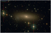 |
Fig. 1 J-PLUS color image of NGC 1023 obtained with the software Trilogy (Coe et al. 2012). To build the color image, the combination of filters (u, J0378, J0410), (J0430, J0515, g), and (J0660, J0861, r, i, z) were used to compose the blue, green, and red components, respectively. The FoV is ≈ 0.1 deg2. |
FWHM values and exposure times for NGC 1023 data in each filter.
3 Methodology
We analyze the data presented in Sect. 2 in two ways: first by compiling a list of GC candidates around NGC 1023 and then by analyzing their stellar population properties.
3.1 Detection of Candidates with GCFinder
To detect GC candidates in J-PLUS images, we developed the semiautomatic pipeline GCFinder, which consists of a python code that detects compact sources in a white image (a sum of frames of the four broadbands g, r, i, and z) and performs a selection of GC candidates based on data quality, shape, color, and magnitude criteria. The code uses Source Extractor (Bertin & Arnouts 1996) and Montage (Berriman et al. 2004), running inside a support folder that also contains necessary files to use GCFinder.
A detailed description of GCFinder and the technical requirements are given in Appendices A and B. In Appendix C, we present the main different methodologies tested for the detection of GC candidates in J-PLUS data before choosing the strategy deployed in GCFinder.
One advantage of GCFinder is that it is a very light code that does not require the modeling of the host galaxy or smoothing filters before the detection of sources. The code is flexible and can be easily adapted to other photometric surveys besides J-PLUS, including the detection of other stellar systems such as ultra-compact dwarf galaxies (UCDs, Phillipps et al. 2001).
We ran GCFinder on the data described in Sect. 2 and we obtained a set of GC candidates (presented in Table 2). We note that a larger number of GC candidates are recovered in redder bands, which is in agreement with what is expected from old stellar objects. We also note that the S/N of blue bands, when compared to the red bands, tends to be lower in J-PLUS.
To measure the detection efficiency, namely, how many GCs the method can recover in the extended light region of the host galaxy’s halo, we compared our detections with the catalog from Kartha et al. (2014), used as a reference.
The NGC 1023 reference catalog of Kartha et al. (2014) originally had 627 objects including faint sources. We note that the work done in Kartha et al. (2014) use data from MegaCam (Lenzen et al. 2003) at the Canada-France-Hawaii Telescope (CHFT), which has a limiting magnitude fainter than T80Cam. In the g-band, we are able to detect objects up to a magnitude of around 24 mag and, for comparison purposes, we exclude objects fainter than the limiting magnitude of our data from the reference catalog. This results in about 200 GC candidates that could be detected within the limiting magnitude of J-PLUS.
By comparing the positions of our GC candidates with the reference catalog (see Fig. 2), we retrieved 188 GCs in common which means that GCFinder detected a large fraction (about 93%) of possible GC candidates. Based on the numbers presented, we estimate that GCFinder does not detect about 7% of expected GCs when compared to the literature. We attribute this difference to the fact that Kartha et al. (2014) detected many globular clusters near the central region of the galaxy since its light central body hampers our ability to detect compact sources, even if modeled (see Appendix C).
On the other hand, we were able to detect 335 new GC candidates with GCFinder thanks to: (1) new outer halo GCs that were identified by taking advantage of the wide field of J-PLUS images and (2) a reduction in the contamination from Milky Way stars, which was possible from the adopted methodology (see Appendix A). From these 335 new GC candidates, 48% of them are located beyond the studied region in previous papers such as Kartha et al. (2014) and the rest of them are in the same halo region explored in the literature; however, these are, on average, fainter than the GC candidates located in same region reported in Kartha et al. (2014).
Number of GC candidates selected per band after the selection criteria are applied.
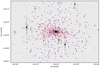 |
Fig. 2 Spatial distribution of GC candidates. In the background we show the white image of NGC 1023 used for the detection of sources. The FoV is ≈0.1 deg2. Red circles represent GC candidates from the reference catalog (Kartha et al. 2014). Blue circles represent GCs in common between GCFinder selection and the reference catalog. |
3.2 Stellar Population Properties
We obtained stellar population properties for our GC candidates via SED fitting. We use the codes DynBaS and TGASPEX (Magris et al. 2015; Mejía-Narváez et al. 2017), adapted to work with the J-PAS, J-PLUS, and S-PLUS filter systems, as illustrated in González Delgado et al. (2021) for mini-JPAS, where TGASPEX was used. Both DynBaS and TGASPEX are non-parametric fitting codes, where the star formation history is expressed as an arbitrary superposition of different simple stellar populations.
This is the first time that the stellar population properties of GC candidates have been derived from J-PLUS data. To investigate the effect of adding narrowbands to the SED fitting, we performed the fits for three different combinations of filters: (a) using only the broad-band filters, (b) using only the narrow–band filters, and (c) using all available filters.
We used the version of the Bruzual & Charlot (2003) stellar population synthesis models described in Plat et al. (2019), referred to as the C&B models hereafter. The C&B models follow the PARSEC evolutionary tracks (Marigo et al. 2013; Chen et al. 2015) and use the MILES (Sánchez-Blázquez et al. 2006; Falcón-Barroso et al. 2011; Prugniel et al. 2011) and IndoUS (Valdes et al. 2004; Sharma et al. 2016) stellar libraries in the spectral range covered by the J-PLUS data. The C&B models are available for 15 different metallicities ranging from log (Z★/Z⊙) = −2.23 to 0.55 (using Z⊙ = 0.017) and run in age from ~ 0 to 14 Gyr. In this paper, we discard the C&B models of supersolar metallicity and use the following 12 metallicities: log(Z★/Z⊙) = −2.23, −1.93, −1.53, −1.23, −0.93, −0.63, −0.45, −0.33, −0.23, −0.08, 0, and 0.07. All the models were computed for the Chabrier (2003) initial mass function.
In DynBaS and TGASPEX, the best-fitting solution is obtained by computing the non-negative values of the coefficients, xtZ, which minimize the merit function:
![Mathematical equation: ${\chi ^2} = \mathop \sum \limits_{\lambda ,tZ}^N {{{{\left[ {F_\lambda ^{{\rm{obs}}} - \sum\nolimits_{t,Z} {{x_t}_Z\,{f_{\lambda ,tZ}}\left( {\tau {\rm{v}}} \right)} } \right]}^2}} \over {\sigma _\lambda ^2}},$](/articles/aa/full_html/2022/08/aa42402-21/aa42402-21-eq1.png) (1)
(1)
used to measure the goodness-of-fit. In Eq. (1),  and fλ,tZ are the observed and model flux in each of the bands, respectively, and
  is the corresponding uncertainty. The sum is done over all the filters (index λ) and the N models (indices t and Z); and N is equal to the number of time steps × the number of metallicities used in the fit.
As described by Magris et al. (2015), in DynBaS, we used N = 3 (hereafter DynBaS3) and we minimized χ2 in Eq. (1), requiring that the three derivatives lead to  . This results in a system of three equations with three unknowns that we solve using Cramer’s rule for all possible combinations of three model spectra. The DynBaS3 solution is then the one with the minimum χ2, subject to the condition xtZ ≥ 0. In TGASPEX we use the non-negative least squares (NNLS) algorithm (Lawson & Hanson 1974) to find the vector, xtZ, that minimizes χ2. For both codes, we used an outer loop to minimize by the dust attenuation, τV.
We remark that both DynBaS3 and TGASPEX provide independent, deterministic solutions (as opposed to statistical solutions) to the SED fitting problem. The TGASPEX solution, in general, with N ≥ 3, contains the DynBaS3 solution. As has been shown in Magris et al. (2015) and Mejía-Narváez et al. (2017), the DynBaS3 and TGASPEX solutions are consistent within errors. González Delgado et al. (2021) showed that the TGASPEX solution is consistent with the solutions obtained by other SED fitting codes, including codes that use a fully Bayesian approach. Prieto et al. (2022, in prep) showed that the deterministic DynBaS3 and TGASPEX solutions are consistent with those derived following a Bayesian treatment for both methods. In this paper, we opt for the deterministic approach for simplicity and because we know from the above-referenced studies that the Bayesian approach does not add any new insights into our problem.
Following González Delgado et al. (2021), we used the frequentist approach of applying a Monte Carlo method to the input (by adding Gaussian noise with observationally defined amplitudes) and repeating the fit many times (≈1000), assuming that the errors in the different bands are uncorrelated. The purpose here is to perform a statistical analysis based on the observed photon-noise and its impact on the results. A probability distribution function (PDF) for each stellar population property was then built by weighting the results from each iteration by the likelihood ℒ ∝ exp(−χ2/2). The inferred value for the property of each GC could then be obtained directly from the corresponding marginalized PDF. In the end, each population property is characterized by its “best” value derived directly by DynBaS3 and TGASPEX, as well as the mean, the median, and the percentiles defining the confidence interval in the distribution. The “best” value is then considered as the best estimate of the unknown “true” value, and its precision is obtained by averaging the precision determined for each cluster from the PDF built as indicated above. Below we describe the properties that are given as results.
The total stellar mass (M) is the total mass of the stellar population. It is calculated directly from the mass converted into stars according to our solutions for the GC, reported as log(M/M⊙).
The luminous stellar mass (M★) is the stellar-mass of the stellar population at present. It is calculated from the mass converted into stars reduced by the mass lost by stars during their evolution, reported as log(M*/M⊙).
With respect to the age of the stellar population, we define the mass-weighted logarithmic age (hereafter mass-weighted age) following Cid Fernandes et al. (2013, Eq. (9)), expressed as:
 (2)
(2)
where μtZ is the fraction of mass of the base element with age t and metallicity Z, reported as 〈log age(yr)〉M. Similarly, the light-weighted logarithmic age (hereafter light-weighted age) is defined as
 (3)
(3)
where  is the fraction of light in the r filter corresponding to the base element with age t and metallicity Z, reported as 〈log age(yr)〉L.
Regarding the metallicity of the stellar population we define the mass-weighted logarithmic metallicity (hereafter mass-weighted Z) as
 (4)
(4)
reported as 〈[Z/Z⊙]〉M, and the light-weighted logarithmic metallicity (hereafter light-weighted Z) as
 (5)
(5)
reported as 〈[Z/Z⊙]〉L.
We define the precision (mean standard deviation, try) for the jth stellar property as
 (6)
(6)
where p84j,i and p16j,i are, respectively, percentiles 84 and 16 of the PDF of the jth property for the ith GC candidate. Example of SEDs chosen randomly are presented in Fig. 3 for the purposes of illustration.
4 Results
4.1 Color Distributions
The study of GC systems in massive galaxies has shown that they can have a bimodal optical color distribution (e.g., Larsen et al. 2001; Peng et al. 2006; Kundu & Zepf 2007). At the same time, several studies have shown that the color-metallicity relation is highly nonlinear (e.g., Yoon et al. 2006; Kim et al. 2021).
We studied the distributions of all possible color-color diagrams with the J-PLUS filter system without mixing broad and narrowband filters (as the broad and narrowband filters were calibrated using different methodologies; see Sect. 2). A total of 25 colors were inspected, with 10 using broad-band and 15 colors on narrowband filters (Figs. 4 and 5, respectively). Gaussian mixture modeling (GMM) was performed on the distributions using the Python library Scikit-Learn (sklearn, Pedregosa et al. 2011), following the procedures from Ivezić et al. (2014). We compare the GMM results obtained for one component (black curve) and two components (purple curve), using the Bayesian information criterion (BIC). The BIC makes assumptions about the likelihood that aims to simplify the calculation of the odds ratio and is useful for estimating the statistical significance of clusters found in the data. Therefore, we assume that lower BIC values are associated with highly significant clusters, following Ivezic et al. (2014, Chap. 5.4).
According to BIC statistics, we find evidence of color bimodality in 17 colors, namely и − g, и − r, и − i, g − r, r − z, i − z, J0378 − J0430, J0378 − J0515, J0378 − J0660, J0378 − J0861, J0410 − J0515, J0430 − J0515, J0430 − J0660, J0430 − J0861, J0515 − J0660, J0515 − J0861, J0660 − J0861. In these cases, the BICs of the GMM with two components have a lower value than the BICs of the GMM with one component. We note that even though the BICs of the GMM with two components are lower than the values for one component, in the cases of u − z, r − i, J0410 − J0430, and J0410 − J0861, the differences of the BICs are too small to be conclusive. In Figs. 4 and 5 we show BIC values for GMM with one and two components as an example.
De Souza et al. (2017) favor the use of a regularized version of BIC, namely, the integrated complete likelihood (ICL). As a sanity check, we repeat the analysis evaluating possible color bimodality using the ICL criterion. According to ICL statistics, we find evidence of color bimodality in ten colors, namely, g − r, r − z, i − z, J0378 − J0515, J0378 − J0861, J0430 − J0660, J0430 − J0861, J0515 − J0660, J0515 − J0861, and J0660 − J0861. In the case of the color J0378 − J0660, the ICL of the GMM with one component has a lower value than the GMM with two components, but the difference is small; hence, we consider this case to be inconclusive. A table (Table D.1) summarising the results from both statistics is presented in Appendix D.
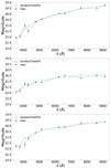 |
Fig. 3 Examples of SED fitting for 3 GC candidates. The observed and synthetic SEDs are presented in black and blue, respectively. The model fits of the two codes are very similar, therefore, they appear superposed in the figure. |
4.2 Stellar population properties
In this section, we present the results of the SED fitting performed on a sub-sample of 171 GC candidates. This subsample consists of only GC candidates with measured magnitudes in all bands. The codes and models used are those described in Sect. 3.2.
The uncertainties of the fits were estimated according to Eq. (6) in Sect. 3.2, extending over the N = 171 GC candidates. In Table 3 we list the resulting values of σj The fits reported were performed for AV = 0, the value of 〉σ(Av)〈 listed in Table 3 gives an indication of the error of this assumption.
Stellar masses. Figure 6 shows that the distributions of the total mass obtained with TGASPEX and DynBaS3 are consistent, and range from below 103 to above 106 M⊙, with a peak around 105.5 M⊙. Given that GC masses are known in the range 104– 106 M⊙ (Brodie & Strader 2006), we interpret the tail towards low mass to be indicative of contaminants (false positives) in our cluster-candidate catalog. Such contaminants represent a negligible fraction, only 5% of our sample of GC candidates. It is unclear at this point if the more massive systems (stellar mass >106 M⊙) are GCs or UCDs (Phillipps et al. 2001). These low-mass candidates are also intrinsically fainter, which results in lower S/N SEDs. Regarding the distributions retrieved from different filter sets, including the narrow–band filters in the fits has the effect of broadening the distribution of the “best” mass values.
Ages. Figure 7 shows the distributions of our fit results for the mass-weighted and light-weighted ages. Old-age clusters, with ages ≈10Gyr dominate the distributions for all filter combinations (narrowband only, broadband only, broad and narrowbands combined), with a secondary peak occurring at ages ≈ 9 Gyr. For reasons that remain unclear at this moment, this second intermediate age peak is less pronounced when only the narrowbands are used in the fit. This may be related to the choice of sub-sample selected to be analyzed via SED fitting, where only the GC candidates with all filters measured were included. DynBaS3 retrieves a higher fraction of old GCs than TGASPEX. We interpret the tail toward the youngest ages (log age < 8) as being produced by contaminants present in our candidate catalog.
Metallicities. Figure 8 shows the distributions of our fit results for the “best” values of mass-weighted Z and light-weighted Z. A clear bimodal distribution of metallicities is seen in most combinations of code and filter set, while the results of light and mass-weighted Z from TGASPEX obtained only with narrowbands show three modes, indicating three different populations. A stronger tail at low metallicities is derived when only the broad–bands are used. We interpret this result as evidence that the narrowbands help to constrain the metallicities. It is unclear at this point how the metallicity distributions are bimodal when we only find evidence of color bimodality in part of the studied colors. A possible channel for this could be a non-linear color-metallicity relation, as already presented in papers by, for instance, Yoon et al. (2006), Cantiello & Blakeslee (2007) and Fahrion et al. (2020). As in other galaxies, we interpreted the two families of metal-poor and metal-rich GCs to be related to two mechanisms or episodes of star formation (e.g., Brodie & Strader 2006), although we do find evidence of three populations when using the narrowband only along with TGASPEX.
Stellar masses versus ages. We explore the possibility of correlations among the derived parameters. The only correlation identified is seen between the stellar mass and light-weighted ages, as illustrated in Fig. 9. A correlation is also present between stellar mass and mass-weighted ages, albeit less clear.
Pfeffer et al. (2018) presented globular cluster models in the context of E-MOSAICS project. These models describe the formation, evolution, and the disruption of this class of objects. In their work they find that based on their models and simulations most low-mass clusters were disrupted at redshift 0, therefore, they concluded that clusters with higher mass are more likely to survive until the present time, which results in old GC populations having a higher characteristic mass when compared with younger GCs. Therefore, we attributed the relation found in this work to the same processes found in Pfeffer et al. (2018), but we also note that we do not calculate ages for all GCs in NGC 1023; therefore, our results could be affected by selection effects that are not well characterized.
Precision (mean standard deviation) of the stellar population properties derived with the TGASPEX code.
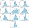 |
Fig. 4 Color distribution computed using broad-band filters only. The curves represent the unimodal (black) and bimodal (purple) distributions returned by the GMM analysis. We also show in blue and red dashed lines the two peaks that compose the bimodal distribution. BICs values for GMM with one and two components are shown as an example. |
4.3 Specific Frequency
The specific frequency (SN) of the GC population of a galaxy represents the total number of GCs per unit of host galaxy luminosity. Following Kartha et al. (2014), we adopted MV = −21.07 ± 0.06 and we based our calculations on the GCLF a NGc = 553 ± 60, which was used to determine the Sn. We calculated SN = 2.1 ± 0.2, which is consistent with the SN = 1.8 ± 0.2 reported in Kartha et al. (2014) and with SN = 1.7 ± 0.3 presented in Yong et al. (2012). Our Sn is also consistent with estimations for lenticular galaxies (2 < SN < 6, Kundu & Whitmore 1998; Elmegreen 2000).
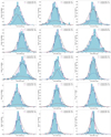 |
Fig. 5 Color distribution computed using narrow–band filters only. The curves represent the unimodal (black) and bimodal (purple) distributions returned by the GMM analysis. We also show in blue and red the two peaks that compose the bimodal distribution. The BIC values for GMM with one and two components are shown as an example. |
5 Discussion
In this section, we discuss the results shown in Sect. 4 with the aim of connecting the observed properties of the GC system with the evolution of NGC 1023.
5.1. Accretion History of NGC 1023
The fact that we can identify bimodal distributions in metallicities from the SED fitting analysis from Sect. 4.2 could be evidence that there are at least two subpopulations of GCs in the galaxy.
Li & Gnedin (2019) used a novel cluster formation model on a simulated galaxy of the same size as the Milky Way and observed that GC candidates tend to form during major merger events. The merger-induced GC formation scenario has been discussed in various recent articles (Li & Gnedin 2014; Choksi et al. 2018; Choksi & Gnedin 2019).
We can further investigate this scenario by studying age-metallicity relations. In Fig. 10, we compare the age-metalliticy relation (hereafter, AMR) obtained from our results to three E-MOSAIC simulations (Pfeffer et al. 2018) from Kruijssen et al. (2019a). We choose three simulations that have halo masses comparable to the halo mass of NGC 1023, adopting the masses from Alabi et al. (2016) and Bílek et al. (2019).
The comparison in Figure 10 is useful for getting a handle on the epoch of GC assembly in the NGC 1023. We note that the AMR of MW023 is in better agreement with the AMR of NGC 1023 GC candidates. We also note that our AMR has outliers, similar to the ones found in MW014. Our results thus favor the accretion histories of simulations such as MW014 or MW023, while ruling out histories such as that of MW016. The AMR of GC candidates, when compared with the simulations, indicate that NGC 1023 likely experienced an initial and rapid phase of star formation that might have formed the majority of the GC candidates; this is supported by the fact that a large number of GC candidates were formed early in galaxy evolution, considering that the age distribution has a dominating peak at ≈1010 yr, in agreement with results from Kruijssen et al. (2019a).
We also note a probable broad AMR, where the GC candidates have a wide range of metallicities. Nevertheless, there is a caveat regarding our interpretation of a broad AMR, as the selection function introduced by GCFinder is not well characterized. As such it remains an open question whether the color cuts applied by the pipeline would introduce distortions in the age-metallicities relation. Kruijssen et al. (2019a) found that a wide range of GC metallicities was related to a wide range of progenitor masses. Therefore, we believe our probable broad age-metallicity relation and our wide range of metallicities imply that NGC 1023 experienced mergers and accretion events in the past, resulting in more than one episode of intense star formation.
This is in sync with what is been discovered about the formation of the Milky Way. Studies on the formation of our Galaxy are motivated by numerous surveys undertaken over the past few years, which have generated huge amounts of data. The Gaia survey (Gaia Collaboration 2016a,b, 2018, 2021), in particular, has been revolutionising our understanding of the Milky Way. Many recent works making use of Gaia have identified stars in the Milky Way that are claimed to have been accreted from dwarf galaxies that no longer exist. In particular, stars that are claimed to have been born in the progenitor galaxies Gaia-Enceladus (Helmi et al. 2018; Belokurov et al. 2018; Das et al. 2020), which is believed to be the last major merger experienced from the Milky Way, from the Sequoia progenitor (Myeong et al. 2019), from Thamnos 1 and Thamnos 2 (Koppelman et al. 2019), and from a structure in the inner Galaxy (Kruijssen et al. 2019b, 2020; Horta et al. 2021), as well as others.
We note that there is evidence drawn from kinematic studies (e.g., Romanowsky et al. 2012; Villaume et al. 2019) and simulations (e.g., Muratov & Gnedin 2010; Choksi et al. 2018) to support accretion events from dwarf galaxies and that the hierarchical assembly of GC systems has been broadly accepted. In particular, the fact that we have only found evidence of color bimodality in some cases is not surprising. We know that GCs trace assembly histories of galaxies and galaxies are likely to undergo many minor and possibly major mergers throughout their lifetimes. In this case, the lack of strong evidence to support bimodality for some colors could be an indicator that more than two subpopulations exist, but we are not able to disentangle them. Puzia et al. (2002) and Blom et al. (2012a,b), for example, found three subpopulations of GCs in the galaxy NGC 4365.
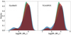 |
Fig. 6 Distribution of stellar masses obtained from SED fitting. The left panel illustrates the results from DynBaS 3, while the right panel shows the results from TGASPEX. The distributions display a broad peak with log Stellar Masses between 5 and 6 M⊙. In red, we show the results obtained using all available filters. Green represents results obtained using broadband filters only. Blue represents results obtained using narrowband filters only. |
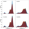 |
Fig. 7 Distribution of logarithmic ages obtained from SED fitting. Upper and lower panels illustrate results from DynBaS 3 and TGASPEX respectively. Left and right panels: results for mass- and light-weighted ages, respectively. Red represents results obtained using all available filters. Green represents results obtained using broadband filters only. Blue represents results obtained using narrowband filters only. |
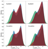 |
Fig. 8 Distribution of metallicities obtained from SED fitting. Upper and lower panels: illustrate results for DynBaS 3 and TGASPEX respectively. Left and right panels: results for mass- and light-weighted Z, respectively. Red represents results obtained using all available filters. Green represents results obtained using broadband filters only. Blue represents results obtained using narrowband filters only. |
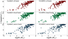 |
Fig. 9 Correlation between ages and masses derived via SED fitting. A trend where the mean ages of the cluster-candidates increase with stellar masses is seen for all combinations of code and filter set. Left and right panels: illustrate the results for DynBaS 3 and TGASPEX, respectively. Red triangles represent results obtained using all bands, green circles represent results when using only the broadband, and blue stars represent results obtained from the narrowband only. |
5.2 Ongoing Interaction with NGC 1023A
NGC 1023 is a barred galaxy in an ongoing interaction with NGC 1023A, a small companion on the outskirts of NGC 1023 at East (Debattista et al. 2002). NGC 1023A was recognised as an independent galaxy by Barbon & Capaccioli (1975) and designated as NGC 1023A by Hart et al. (1980). Capaccioli et al. (1986) classified it as a Magellanic irregular or late-type dwarf galaxy, while Sancisi et al. (1984) from HI observation found that there is a complex kinematics at work. On the other hand, Debattista et al. (2002) found a faster bar pattern speed, which would be not compatible with a scenario of a recent formation of the bar by the interaction with NGC 1023A. Nevertheless, the ongoing interaction may have an effect on the overall NGC 1023 structure as well as on the GCs distribution. A small fraction of the GC population of the NGC 1023 system could be associated with NGC 1023A (Cortesi et al. 2016). Due to the morphology and luminosity of NGC 1023A, a definition of its center is challenging, but we estimate that NGC 1023A is at a projected distance of approximately 6.7 kpc from NGC 1023.
Since NGC 1023 is an early type galaxy the tidal effect could have two different dynamics answers depending on how longer or shorter the encounter time is compared to the galaxy’s internal cross-time (e.g., Aguilar & White 1985, 1986; Binney & Tremaine 2008). For the outer parts, the crossing time could be larger than the encounter time, therefore, they may suffer an impulse response. On the other hand, for the inner parts, the cross-time could be smaller than the encounter time, thus they may suffer a typical tidal response. As a consequence, the central parts can be displaced with respect to the outer ones. These offsets can be up to 20% of the observable radius of the galaxy (Lauer 1986, 1988; Davoust & Prugniel 1988; Combes et al. 1995; González-Serrano & Carballo 2000; Mora et al. 2019; Buzzo et al. 2021).
Buzzo et al. (2021) have shown that the nucleus of the lenticular galaxy NGC 3115 has a displacement of 160 arcsec with respect to the outer parts. They interpret it as the result of a recent pericenter passage with its close small companion. To probe the possibility of NGC 1023 having a similar feature, we performed a similar photometric analysis, following Mora et al. (2019) and Buzzo et al. (2021). We modeled the isophote contours, in r-band, using the ELLIPSE task from IRAF (Jedrzejewski 1987). We let the position angle, ellipticity, and centre of the ellipses to remain free. To quantify the offset of the isophotes, we took as our reference the photometric center of the galaxy. In Fig. 11, we show the radial profile of the offsets at the top panel, while the outermost isophotes and their respective fitted ellipses with their centers are plotted in the bottom panel. It is clear that from ~ 100 arcsec the central part starts to move toward the east-south with respect to the outer parts, the maximum offset is about ~700pc. This nuclear displacement is strong evidence that NGC 1023 and NGC 1023A had recently a pericenter passage, just a few hundred million years ago (Combes et al. 1995; Mora et al. 2019). The orientation of the offset could be used as a strong constraint in a numerical simulation of the dynamic encounter of this pair, since the central part of NGC 1023 must have headed into the east-south direction at the pericenter passage. This would limit the family of possible orbits to model the system, (e.g., Combes et al. 1995; Mora et al. 2019).
We consider the way this interaction could have affected the distribution of the GCs of NGC 1023. To address this question, we calculated the photometric center of the GCs candidates and overlaid it on the bottom panel in Fig. 11. We can see that the photometric center of the GCs candidates follows the same direction as the centers of the outer isophotes. The displacement of the nucleus region with respect to the GCs is ~1600 pc. This behavior is expected based on impulse theory (Aguilar & White 1985, 1986; Binney & Tremaine 2008), since the GCs belong to the galactic halo; thus, they have the greatest crossing times of the galaxy and their nuclear displacement is expected to be the largest.
In addition to this photometric analysis, we studied the residual image from the ellipse model (see Fig. 12). The residual image unveils NGC 1023A and the bar (oriented north-east to south-west) of NGC 1023 (Möllenhoff & Heidt 2001; Debattista et al. 2002), along with two possible relic like-spiral arms. The bar has a radius of ~ 1100 pc. We note that here we are reporting the presence of these relic spiral-like arms for the first time. It is very plausible that the origin of these structures is also due to the interaction with NGC 1023A; in this case, they would be tidal structures. However, one of the formation mechanisms of lenticular galaxies is gas removal from a spiral galaxy, then these relic spiral-like arms could be a fossil record of the progenitor galaxy of NGC 1023. These features can also serve as dynamical constraints for a numerical simulation of the encounter.
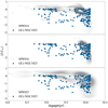 |
Fig. 10 AMR for the NGC 1023 GC system based on DynBaS 3 (blue circles) compared to 3 E-MOSAIC simulations: MW014, MW016, and MW023 from Kruijssen et al. (2019a) (grey contours) that have comparable halo masses to NGC 1023. We observe a (likely) broad AMR of NGC 1023 GC system, where the objects have a broad metallicity distribution and are mainly old. |
6 Summary and Conclusions
In this work, we present the first study on extragalactic globular clusters using J-PLUS data. As a test case, we detected and studied the GC system in NGC 1023 with the 12 bands of J-PLUS. To detect the GC candidates we develop GCFinder, a code that can be applied to current and upcoming wide-field multi-band surveys, such as J-PAS and S-PLUS. The pipeline presents good results within the characteristics of the survey for which it was designed. The end product is a code that can be adapted to other photometric surveys and other types of compact stellar systems, such as ultra-compact dwarf galaxies.
Based on the catalog of GC candidates provided by GCFinder, we performed a study of the stellar population content of a sub-sample of objects, using SED fitting techniques and photometry from broad and narrow–band filters. To calculate the masses, ages, and metallicities of the GC candidates, we used the codes DynBaS3 and TGASPEX adapted to work with the J-PLUS filter system. We also carefully model the light of NGC 1023 to investigate any possible displacement between the outer isophotes and the distribution center of the GC candidates, which is useful for improving our understanding of galaxy evolution. We summarize our main findings as follows.
We identified 523 GC candidates in NGC 1023 using GCFinder, with 335 of them not yet reported in the literature. A significant part of these new GC candidates is located in the outer regions of NGC 1023 thanks to the wide field of view of the J-PLUS images we used. We found a specific frequency of Sn = 2.1 ± 0.2, which is consistent with estimations for lenticular galaxies in the literature.
We investigated the color distributions of the GC candidates, exploring the novel colors provided by J-PLUS. According to BIC statistics, we find evidence of color bimodality in 17 colors (u − g, u − r, u − i, g − r, r − z, i − z, J0378 − J0430, J0378 − J0515, J0378 − J0660, J0378 − J0861, J0410 − J0515, J0430 − J0515, J0430 − J0660, J0430 − J0861, J0515 − J0660, J0515 − J0861, J0660 − J0861), while according to ICL statistics we find evidence of color bimodality in ten colors (g − r, r − z, i − z, J0378 − J0515, J0378 − J0861, J0430 − J0660, J0430 − J0861, J0515 − J0660, J0515 − J0861, J0660 − J0861).
We obtained the masses, ages, and metallicities for 171 GC candidates from SED fitting. We find that the peak of the mass distribution is at 105.5 M⊙. We also find a tail of GC candidates with low masses, which we interpreted as likely contaminants in our list of candidates. It is unclear at this point if the more massive systems (stellar mass >106 M⊙) are GCs or UCDs.
The mass-weighted and light-weighted age distributions cover a wide range of ages, with a dominant population at ≈1010 yr. The mass-weighted and light-weighted metallicity distributions of the GC candidates are bimodal in most of the cases (combining different filter sets and codes) and, in a minority of cases, we find three peaks. We note that the inclusion of narrow–band filters helps to constrain the metallicities. These results indicate that there are subpopulations of GCs in NGC 1023 that could exist due to accretion events or different epochs or mechanisms of star formation in the galaxy.
We identified a correlation between light-weighted ages and stellar masses, where older GCs tend to be more massive. This suggests that massive GC candidates in NGC 1023 are more likely to survive the turbulent history of the host galaxy than less massive objects, which is in agreement with the literature on GC systems of galaxies.
The age-metallicity relation is likely to be rather broad. A comparison with simulations shows evidence of a likely initial rapid phase of star formation, responsible for the formation of the majority of the GCs. Works in the literature (e.g., Kruijssen et al. 2019a) have shown that a wide range of GC metallicities is related to a wide range of masses of progenitor galaxies. Therefore, the broad AMR we find is also evidence of past accretion events experienced by NGC 1023.
We also detected that the photometric center has a displacement of ~700pc and ~1600pc with respect to the outer isophotes and the GC candidate distribution center, respectively. The offsets could be the result of ongoing interaction between NGC 1023 and NGC1023A. These effects are in excellent agreement with impulse theory (Aguilar & White 1985, 1986; Binney & Tremaine 2008).
The residual map obtained from the photometric model of NGC 1023 unveils two spiral-like arms. These structures are probably due to the NGC 1023 interaction with the NGC1023A satellite galaxy.
From our main findings, we conclude that it was possible to retrieve new and valuable information about the evolutionary past of NGC 1023 as observed by J-PLUS. The multiple GC populations, relic spiral arms, and displacement between the photometric center of the GC candidates and the isophotal center that we report in this work support a formation history for NGC 1023 that involved several minor mergers and group harassment, causing a transformation from a spiral to the lenticular galaxy that currently exists.
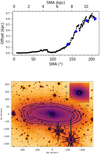 |
Fig. 11 Displaced nucleus of NGC 1023. Top panel: offset radius profile with respect to the photometric center of the galaxy. Bottom panel: selected outer isophotes (in black) with their respective fitted ellipses (blue) are overplotted on r-band image. The blue pluses are their respective centers, while the red point is the photometric center of the galaxy, and the green point is the photometric center of GCs candidates. The top-right inset is a zoom-in of the inner part to better see the displacements. The blue points in the offset radius profile are the offsets for the selected isophotes. |
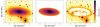 |
Fig. 12 Photometric model for NGC 1023. Left panel: R-band image. Middle panel: ellipse model. Right panel: residual map, with NGC 1023A revealed, together with two spiral arms and an inner bar. |
Acknowledgements
We thank the referee for the valuable comments and careful revision that helped us to improve this manuscript. We thank Diederik Kruijssen for sharing the AMRs presented in Kruijssen et al. (2019a). D.B.S. acknowledges Paula Jofré for the scientific discussions, mentoring, all the support, and for the constant and invaluable availability. D.B.S. also acknowledges Fundação de Amparo à Pesquisa do Estado de São Paulo (FAPESP) process number 2017J00204-6 for the financial support provided for the development of this project. P.C. acknowledges support from Conselho Nacional de Desenvolvimento Científico e Tecnológico (CNPq) under grant 310041/2018-0 and from Fundação de Amparo à Pesquisa do Estado de São Paulo (FAPESP) process number 2018J05392-8. A.C.S. acknowledges funding from CNPq and the Rio Grande do Sul Research Foundation (FAPERGS) through grants CNPq-403580/2016-1, CNPq-11153/2018-6, PqG/FAPERGS-17/2551-0001, FAPERGS/CAPES 19/2551-0000696-9 and L’Oréal UNESCO ABC Para Mulheres na Ciência and the Chinese Academy of Sciences (CAS) President’s International Fellowship Initiative (PIFI) through grant E085201009. G.B. acknowledges financial support from the National Autonomous University of México (UNAM) through grant DGAPA/PAPIIT IG100319 and from CONACyT through grant CB2015-252364. J.V. acknowledges the technical members of the UPAD for their invaluable work: Juan Castillo, Tamara Civera, Javier Hernández, Ángel López, Alberto Moreno, and David Muniesa. J.A.H.J. acknowledges Fundação de Amparo à Pesquisa do Estado de São Paulo (FAPESP), process number 2021J08920-8. A.E. acknowledges the financial support from the Spanish Ministry of Science and Innovation and the European Union – NextGenerationEU through the Recovery and Resilience Facility project ICTS-MRR-2021-03-CEFCA and from Conselho Nacional de Desenvolvimento Científico e Tecnológico (CNPq) under grant 313285/2020-9 D.A.F. thanks the ARC for financial assistance via DP170102344. Y.J.-T has received funding from the European Union’s Horizon 2020 research and innovation program under the Marie Skłodowska-Curie grant agreement No 898633. Y.J-T. also acknowledges financial support from the State Agency for Research of the Spanish MCIU through the “Center of Excellence Severo Ochoa” award to the Instituto de Astrofísica de Andalucía (SEV-2017-0709). Based on observations made with the JAST80 telescope telescope/s at the Observatorio Astrofísico de Javalambre, in Teruel, owned, managed, and operated by the Centro de Estudios de Física del Cosmos de Aragón. We thank the Centro de Estudios de Física del Cosmos de Aragón for the allocation of the Director’s Discretionary Time to this program. We thank the OAJ Data Processing and Archiving Unit (UPAD) for reducing and calibrating the OAJ data used in this work. Funding for the J-PLUS Project has been provided by the Governments of Spain and Aragón through the Fondo de Inversiones de Teruel; the Aragón Government through the Research Groups E96, E103, and E16_17R; the Spanish Ministry of Science, Innovation, and Universities (MCIU/AEI/FEDER, UE) with grants PGC2018-097585-B-C21 and PGC2018-097585-B-C22; the Spanish Ministry of Economy and Competitiveness (MINECO) under AYA2015-66211-C2-1-P, AYA2015-66211-C2-2, AYA2012-30789, and ICTS-2009-14; and European FEDER funding (FCDD10-4E-867, FCDD13-4E-2685). The Brazilian agencies FINEP, FAPESP, and the National Observatory of Brazil have also contributed to this project. This work has made use of the computing facilities of the Laboratory of Astroinformatics (IAG/USP, NAT/Unicsul), whose purchase was made possible by the Brazilian agency FAPESP (grant 2009/54006-4) and the INCT-A. This work has made use of data from the European Space Agency (ESA) mission Gaia (https://www.cosmos.esa.int/gaia), processed by the Gaia Data Processing and Analysis Consortium (DPAC, https://www.cosmos.esa.int/web/gaia/dpac/consortium). Funding for the DPAC has been provided by national institutions, in particular, the institutions participating in the Gaia Multilateral Agreement. The Pan-STARRS1 Surveys (PS1) and the PS1 public science archive have been made possible through contributions by the Institute for Astronomy, the University of Hawaii, the Pan-STARRS Project Office, the MaxPlanck Society, and its participating institutes, the Max Planck Institute for Astronomy, Heidelberg and the Max Planck Institute for Extraterrestrial Physics, Garching, The Johns Hopkins University, Durham University, the University of Edinburgh, the Queen’s University Belfast, the Harvard-Smithsonian Center for Astrophysics, the Las Cumbres Observatory Global Telescope Network Incorporated, the National Central University of Taiwan, the Space Telescope Science Institute, the National Aeronautics and Space Administration under Grant No. NNX08AR22G was issued through the Planetary Science Division of the NASA Science Mission Directorate, the National Science Foundation Grant No. AST-1238877, the University of Maryland, Eotvos Lorand University (ELTE), the Los Alamos National Laboratory, and the Gordon and Betty Moore Foundation.
Appendix A Identifying GC Candidates: GCFinder Pipeline
Appendix A.1 Handling the Host Galaxy
Historically, the first step when investigating extragalactic globular clusters is modeling the surface brightness of the host galaxy (e.g., Forbes et al. 2014; Kartha et al. 2014; Cho et al. 2016). This is done to enhance the detection of point-like objects inlaid in the extended galaxy halo light. Following this approach, we first attempted to remove the smooth galaxy light profiles from the individual images. To perform that step, we carried out numerous tests with a range of software, from ELLIPSE (Tody 1993), ISOFIT (Ciambur 2015), and GALFITM (Bamford et al. 2011; Häußler et al. 2013), as well as median smoothing technique. One challenge that we found was in NGC 1023 having a very large image size of approximately 700 X 260 pixels (≈ 0.004 square degrees), which makes the modeling very time-consuming as well as computationally consuming. The other main challenge we found was that NGC 1023 has a companion that overlaps with it in the image. As a consequence, when we subtract the model from the observed image, the residual image does not offer the necessary level of quality. More details about the different methods tested as well as about intermediate results are presented in Appendix C.
From the several tests we carried out, we learned that we were not able to retrieve GCs projected over the central brightest regions of the galaxy, even when modeling and subtracting the galaxy’s two-dimensional light profile. We therefore explored alternative methods for retrieving GCs in J-PLUS.
Appendix A.2 GCFinder
To detect and select GC candidates in J-PLUS-like images, we developed a pipeline called GCFinder, which consists of an approach that does not require modeling the host galaxy and is based on a careful detection of GC candidates using Source Extractor (Bertin & Arnouts 1996) as well as criteria based on the data quality, morphology, color, and magnitude of the objects. Such GCs are not detected a priori by the data reduction pipeline of J-PLUS (JYPE, Cristóbal-Hornillos et al. 2014), therefore, to develop a straightforward way to detect and select these objects is fundamental to perform GC studies for a large sample of galaxies.
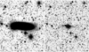 |
Fig. A.1 Illustration of the Source Extractor method. Left panel: Zoom on the NGC 1023 image. Right panel: Illustration of the way Source Extractor interprets the image with the chosen input parameters. |
White image: The detection image is a “white” image, that is, an image originated from the sum of frames of four broadbands (g, r, i, and z), while the photometry was performed in each band independently. We do not use the u filter because it has a low response (see Cenarro et al. 2019) and it could include noise to the white image. The use of a white image increases the chances of detecting faint sources, which are harder to detect in separate bands. To construct the white images, the Montage package (Berriman et al. 2004) was applied and included in the pipeline. With the use of Montage, it is possible to align the images before combining them, to build white images without the displacement of frames of different bands and it is also possible to perform a background correction on the studied images. It is important to avoid any displacement of frames because it could introduce an effect of expanding the objects and, in addition, it could produce fake detections since light could be detected in false positions. This methodology was adopted to increase the signal-to-noise ratio of the sources and thus enhance the level of object detection. To prevent possible noise associated with the narrowband images from being introduced in the detection image, only the broadband images were adopted in the construction of the white images.
Detection of point-like sources as GC candidates: To perform a detection of GCs that also includes objects close to the center of NGC 1023, we performed extensive testing of the different input parameters of Source Extractor to optimize our detection. We identify three key input parameters of Source Extractor to perform the detection of GCs under these conditions: BACK_SIZE, BACK_FILTERSIZE, and PHOT_AUTOPARAMS. In particular, BACK_SIZE determines the pixel size of the area used to estimate the background and is one of the most important parameters. If the BACK_SIZE is too small, the background estimate can be affected by the presence of objects and noise and it is also possible that part of the surrounding galaxy light is absorbed in the background map. If the BACK_SIZE is too large, it does not consider small variations in the background. BACK_FILTERSIZE is the parameter that controls the size of the filter used to estimate the background. Finally, PHOT_AUTOPARAMS is the parameter that controls the elliptical opening used for object detection.
We note that when these key parameters are included as a function of the FWHM of each image, Source Extractor does not consider the extended light profile of the galactic halo in its detection, making it possible to recover the GCs in this inner region of NGC 1023 as shown in Figure A.1. The functions of the adopted BACK_SIZE, BACK_FILTERSIZE, and PHOT_AUTOPARAMS can be seen in Equations A.1, A.2, and A.3, respectively. For more details about the input parameters of GCFinder, were refer to Appendix B.
 (A.1)
(A.1)
 (A.2)
(A.2)
 (A.3)
(A.3)
A factor of 1.05 appears to increase the FWHM value by 5% to compensate for variations throughout the field of the images since the Point Spread Function (PSF) in the images used in the work is not homogenized. In this work, we always use magnitude MAG_AUTO.
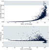 |
Fig. A.2 Illustration of the selection by quality and shape (phase 1). Top panel: Magnitude error as function of the source magnitude. Bottom panel: FWHM of the sources as a function of the source magnitude. Objects in the gray area have been discarded, following the selection criteria described in the text. |
After detecting all sources using Source Extractor in dual mode, the pipeline performs the selection of GC candidates. We adopt criteria based on the shape, magnitude, color, and data quality of the objects.
Phase 1 - Selection by quality and shape: The first selection done by GCFinder refers to the data quality and shape of objects (hereafter Phase 1), adapted from Cho et al. (2016). Phase 1 is done using the white image only. In the case of detections done in the white image, we adopt as Source Extractor input values those associated with the band with the worst PSF. The catalogs generated in this Phase 1 are used to select data quality and object format. We set white source magnitude error (MAGERR_AUTO) < 0.2 to have an S/N > 5 on the selected data. With the creation of the white image, we observe that few objects are excluded at this stage since the adopted methodology improves the S/N of the data, as can be seen in Figure A.2. We make one more data quality selection to exclude objects that were saturated or that were too close to the edge of the images. This type of object has compromised photometry, which can affect the magnitude and color selection that is performed in the following phases of the pipeline. For this, we adopt the Source Extractor FLAGS output parameter < 4, in agreement with Cho et al. (2016). To select only compact objects, we visually set limits for the FWHM, as can be seen in Figure A.2. The region identified in this Figure corresponds to objects that are point-like sources. Such a selection makes it possible to exclude detections that are possibly galaxies. An example of selection using such criteria is shown in Figure A.2.
Phase 2 - Selection by color: The next selection done was related to the color of objects (hereafter Phase 2). Phase 2 is done using the individual images of g, r, and i bands. At this point, we establish threshold values for the colors of the selected objects, to separate possible GCs from other objects, such as passive galaxies and low-mass stars. To do this, we make a selection on a color-color diagram of g − r versus r − i. We chose to use these colors since the number of detections is high in each band. In this diagram, a concentration of objects appears in a well-defined region of the image, which we refer to as the main branch. To select objects in color r − i, we exclude sources that were far from the main branch, and to select objects in color g − r, we exclude objects in the region where there is a more accentuated growth in the value of color r − i. An example of the cut established for NGC 1023 can be seen in Figure A.3. Objects in the region where the more accentuated growth of the color r − i begins are possible low-mass stars (Finlator et al. 2000) and high redshift galaxies (Goto et al. 2002; Prakash et al. 2015). The chosen region also corresponds to the same color interval from the majority of GC candidates reported in Kartha et al. (2014), which we also show in Figure A.3.
Phase 3 - Magnitude limit cut: The third selection (hereafter Phase 3) is performed according to the magnitude of the objects in g-band. In this last step in the selection of GC candidates, very bright objects were excluded to clean our sample of Galactic stars, objects between the Milky Way and NGC 1023, as well as possible ultra-compact dwarf galaxies (UCDs, Phillipps et al. 2001), for example. For this purpose, the magnitude of one of the largest GCs from Forbes et al. (2016), which is a reference catalog containing only spectroscopically confirmed globular clusters and other compact stellar systems, was used as a reference. Its absolute magnitude in the g-band was calculated from the distance of the galaxy and adopted as the typical magnitude of the brightest GCs (see Figure A.4).
Phase 4 - Matching the GC candidates in all bands: At the end of all these selection steps, a final catalog with GC candidates is created (hereafter Phase 4). Afterward, matches are made from the final selection catalog with the detection catalogs of each band, using STILTS (integrated into the pipeline, Taylor 2006), to obtain the GC candidates in each band. This procedure is necessary since the Source Extractor input parameters of the detection image and photometric images are different, therefore, the same objects do not necessarily have the same ID in all bands.
The pipeline - The current version of the pipeline GCFinder consists of a code in python that performs the process described in the previous paragraphs in a semiautomatic way. The code run inside a support folder prepared with the necessary directories for the correct functioning of Montage and the files for the correct functioning of the Source Extractor. For more details, we refer to Appendix B.
Appendix A.3 GCFinder Performance
Appendix A.3.1 Comparison with Gaia EDR3 Data
In terms of the possible contamination by field stars, the contaminants have a shape, color, and magnitude in the g-band equivalent to those of the GCs and we were not able to exclude such objects using the techniques presented in this work – even if the selection criteria adopted in GCFinder encompass the main photometric selection techniques adopted in the literature.
A sanity check was carried out to evaluate the foreground stars in our sample, namely, via an inspection of the parallax of the GCs selected by GCFinder. First, we cross-matched our catalog of GC candidates with Gaia EDR3 (Gaia Collaboration 2016b, 2021) data to acquire parallax measurements. From the 523 objects selected by GCFinder, we found only 153 in Gaia EDR3 considering a searching radius of 1 arcsec. Then we verified whether the parallax values were compatible with zero within 3 sigmas (which indicates that the GC candidates are at a distance that is compatible with extragalactic objects). In general, all the GC candidates found in Gaia EDR3 have large parallax uncertainties (always larger than 0.4 mas), meaning all their parallax values are compatible with zero.
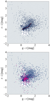 |
Fig. A.3 Illustration of the selection by color (phase 2). Top panel: Selection of the GC candidates on the color-color diagram of the detections. Objects in the gray area have been discarded. A red line was included to guide the eye. Bottom panel: same as top panel with GC candidates also presented in Kartha et al. (2014) in magenta. |
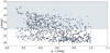 |
Fig. A.4 Adopted upper limit in terms of magnitude (phase 3). Objects in the gray area have been discarded. |
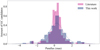 |
Fig. A.5 Distribution of parallaxes for the GC candidates as obtained from Gaia EDR3. The blue distribution corresponds to the candidates of the present wok and magenta shows the distribution of GC candidates identified by Kartha et al. (2014). |
In Figure A.5, we compare the distribution of parallaxes from our catalog with the distribution of GC candidates in Kartha et al. (2014). From the 627 GC candidates presented in Kartha et al. (2014), we found only 164 in Gaia EDR3 considering a search radius of 1 arcsec. The parallax distribution of objects from the literature is narrower than the distribution of GC candidates from GCFinder, but the range covered by the two data sets is similar. Therefore, using our methodology, we obtain a catalog of GC candidates that is consistent with previous articles, with the advantage of not requiring modeling to remove the host galaxy light, either through modeling of the host galaxies’ structural components or through median filtering.
This shows that the pipeline could be easily applied automatically in surveys such as J-PLUS, J-PAS, and S-PLUS. In turn, this could potentially generate large catalogs of GC candidates, especially in the outer halo regions and for spectroscopic follow-up.
Appendix A.3.2 Comparison using Colors
To explore the nature of the new GC candidates found in this work, we analyze their colors and compared them with GCs detected by GCFinder that were also reported in Kartha et al. (2014).
Figure A.6 compares the distributions of colors of GC candidates selected by GCFinder and those of Kartha et al. (2014). We observe that there are color shifts (e.g., u − g, u − r, u − z). The GC candidates that are not found in Kartha et al. (2014) are bluer, which is consistent with metal-poor halo GCs. Although the distribution profile is not the same among the two groups, there is no clear separation between them.
We note that many papers in the literature use machine learning to classify objects. In particular, López-Sanjuan et al. (2019) study the star galaxy separation of objects in J-PLUS data considering their morphology, Wang et al. (2021) build a supervised machine learning algorithm to classify objects (stars, galaxies, and quasars) in J-PLUS, Costa-Duarte et al. (2019) use machine learning to perform star galaxy separation in S-PLUS data while Nakazono et al. (2021) train a random forest classifier and provided catalogs of stars, galaxies, and quasars also in S-PLUS survey. We believe that such approaches would be complementary in the case of identification of GCs, but this is not the objective of the current work. Having a pipeline based only on astrophysical selection is useful for the purpose of characterizing the properties of this class of objects in new surveys and is also efficient, as shown. Our goal for our work is also for it to serve as a training base for future pipelines based on machine learning techniques.
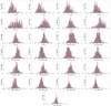 |
Fig. A.6 Density distributions of colors based on J-PLUS filters. Magenta: Color distribution of GC candidates identified by GCFinder that are also present in the reference catalog (Kartha et al. 2014). Grey: Color distribution of GC candidates identified by GCFinder that are not present in the reference cátalos. |
Appendix B Structure of the Pipeline GCFinder
Appendix B.1 Technical Requirements
For the GCFinder pipeline to work, the following resources must be installed on your computer:
Python 2.7
Montage
Source Extractor
STILTS
The pipeline was developed and tested only on the Unix system; more precisely, on Ubuntu 16.04. The pipeline needs a processing time of approximately 7 minutes, with 70 % of this time being consumed in the construction of the white image. This information comes from results obtained with a computer with 4 GB of RAM and an Intel core I5 processor. The pipeline has no special requirements for RAM or processing capacity of the machine used. However, the original J-PLUS images have a large field (9500 pixels × 9500 pixels, ≈ 2 deg2) and we only worked with images cropped in the region of the galaxy, so the studied images have smaller fields. As Montage has been integrated into the pipeline, working with the original images makes the necessary processing time longer and computers with little RAM face difficulties in the white image construction stage. Considering what was studied in this work, this particular result is very satisfactory, given that the main difficulty we face was the fact that many packages for modeling and removing the light profile of the galaxy requires hours of runtime on machines with great processing power.
Appendix B.2 Inputs required for Pipeline Operation
Before the GCFinder pipeline starts working, the user must include the images of all bands in a specific directory inside the support folder where the code is inserted and provide a file with the zero-point values for each band. When the pipeline starts working, the user is asked to provide the path to the pipeline directory, so that the code can perform the necessary operations between files and folders. During code execution, three more pieces of information are requested. The first one is the FWHM cutoff that must be used, the second one is the limits in the color-color diagram, and finally, the distance from the galaxy so that the calculation of the magnitude cutoff is carried out. The FWHM and color cuts remained interactive, as the distribution of such quantities in the graphs might be particular to each galaxy. Keeping these steps interactive ensures better results and greater user control.
Appendix B.3 Pipeline Outputs
The final product of the GCFinder pipeline consists of catalogs of GC candidates for each band, with information on coordinates and magnitudes. In addition, a file is generated with the number of GC candidates in each band, to facilitate the visualization of the results. The pipeline also provides intermediate catalogs at the end of each execution step and provides figures like those presented in the previous sections with the criteria adopted in each selection. This allows the user to have control of what is done during the code execution and access to partial results.
Appendix C Other Methods Tested for Dealing with the Host Galaxies
Here, we present more details about the different methods tested to detect globular clusters in J-PLUS images.
Appendix C.1 ELLIPSE and BMODEL Method
ELLIPSE and BMODEL (Tody 1993) are packages that are widely used with the objective of removing extended light profiles of galaxies so that globular clusters can be detected. ELLIPSE is an IRAF task that adjusts elliptical isophotes in images of galaxies, having as input a set of parameters based on the geometry of the object that is modeled and as output a table with information about the fit. BMODEL creates a noise-free two-dimensional photometric model of the galaxy built from the data table generated by ELLIPSE. After making the model of the galaxy, the Imarith task present in IRAF (Tody 1993) was used to subtract from the original image of the galaxy the constructed light model to obtain a residual image from which GC candidates would be selected. All input parameters were determined through several tests with the images and visually evaluating the quality of the residual image obtained.
As mentioned in the literature (Ciambur 2015), we observe that the simpler the galaxy, the better the residual image formed from this process. This is because the galaxy modeling potential of ELLIPSE and BMODEL is greater for simple galaxies. Since the objective of this work was to create a pipeline as automated as possible, ELLIPSE was not used interactively in this work.
Appendix C.2 ISOFIT and CMODEL Method
ISOFIT and CMODEL (Ciambur 2015) are new versions of ELLIPSE and BMODEL, respectively. Thus, the functioning of these IRAF tasks is analogous to what was presented in the previous section. The modeling of more complex galaxies carried out with ELLIPSE and BMODEL has limitations when the object of study is a galaxy with a certain degree of complexity (such as arms or bars).
However, the updated versions of ISOFIT and CMODEL generate smaller residues for the cases of galaxies that present a more complex structure (Ciambur 2015). ISOFIT is more efficient than ELLIPSE for modeling more complex galaxies because there is the possibility of working with higher harmonics (Jedrzejewski 1987; Bender et al. 1988; Ciambur 2015). The number of maximum possible harmonics can be influenced by the quality of the images studied3.
Input parameters were obtained in the same way as with ELLIPSE, just selecting input parameters without using the interactive mode and performing several tests to determine the parameters that would generate the best possible residual images. We have observed that ISOFIT and CMODEL create better residual images, improving our detections of GC candidates.
Appendix C.3 GALFITM Method
GALFITM (Bamford et al. 2011) is a software that models and removes the light profile of galaxies. It was developed within the context of the Megamorph project (Bamford et al. 2011), which created new versions of the GALFIT (Peng et al. 2002) and GALAPAGOS (Barden et al. 2012) tools that are capable of modeling galaxies in multiple bands. Thus, the Megamorph project software builds galaxy models depending on the wavelengths of the filters used. Furthermore, GALFITM encompasses the morphology of galaxies in the modeling process. Several tests were performed with different input parameters and the quality of the residual images obtained was visually assessed. An example of a residual image obtained using this method is presented in Figure C.1.
GALFITM is much more automatic than ELLIPSE and ISOFIT, so that among all the software studied to model and remove the light profile of the galaxy, it proved to be the most suitable for this work. Due to the processing power required to create the models, we use the uv100 machine from the Astroin-formatics Laboratory at IAG-USP4 for the Brazilian astronomical community (LAi). Using the large processing capacity at LAi, we see that GALFITM required at least 2 hours to process a dataset if an exponential disk profile was used. After performing tests with GALFITM, we conclude that non-parametric alternatives should be tested for this work, since using classic interactive software was unfeasible for our purpose. Using classic automatic software also requires a lot of time and processing power from the machine used, adding an unwanted level of complexity to the pipeline. As additional methods, we tested median smoothing as well as direct detections of objects in the image only using Source Extractor.
Appendix C.4 Median Smoothing Method
The median smoothing technique consists of applying a filter to an astronomical image. In this technique, windows are created on the studied images and the central pixel is replaced by the median of all pixels in the window. To perform median smoothing, the median feature of the IRAF package was used (Tody 1993). The window size (xwindow and ywindow parameters) chosen was 25 for each axis.
Once the filtered image was created, it was subtracted from the original image using the Imarith resource, also from the IRAF package. As a result, an image without the extended light profile of the galactic halo was obtained. In this image, however, the central part of the galaxy is not removed. An example of a residual image obtained using this method is presented in Figure C.2.
Appendix C.5 Source Extractor Method
The Source Extractor (Bertin & Arnouts 1996) performs photometry of astronomical objects (mainly extragalactic ones) and is used in the JYPE pipeline (Cristóbal-Hornillos et al. 2014), responsible for the J-PLUS data reduction. By using it in our pipeline, we ensure that the catalogs produced by our code are compatible with JYPE’s catalogs. The methodology applied when using this method is described in detail in Appendix A. By adopting adequate values of BACK_SIZE, BACKFITLER_SIZE, and PHOT_AUTOPARAMS, we realize that Source Extractor does not consider the extended light profile of the galactic halo in its detection, making it possible to recover the GC candidates in this region. This methodology works because the background subtraction of Source Extractor first estimates the mode using the median of each cell of size BACK_SIZE and then computes the median from those modes in larger cells of size BACK_FILTERSIZE. BACK_FITLERSIZE. This final combination of the mode and median filtered image is then subtracted from the original one before the detection procedure. Therefore, the Source Extractor method serves (in a way) as a combination of the mode and median smoothing procedure.
Appendix C.6 Comparison of Applied Methods
As mentioned above, NGC 1023 has a companion that appears overlapped to it in the image, which makes this galaxy challenging to model. We consider GALFITM the software more suitable for our proposes, since it is more automatic than ISOFIT and ELLIPSE and also because it builds the profile of the galaxies in all bands together. On the other hand, GALFITM requires considerable time to run. Due to the speed and ease of the median smoothing technique and the Source Extractor method, we decide to investigate them based on their efficiency in detecting GCs.
The detection efficiency consists of how many GCs the method can recover in the extended light region of the host galaxy’s halo. To perform this comparison, we use the catalog of GC candidates by Kartha et al. (2014), with 627 objects. We used the results obtained with ISOFIT and CMODEL (Ciambur 2015) to represent the traditional methods of modeling and removing the light profile of the galaxy, as the residual images obtained with this method are of a higher quality. We observed that when removing the light profile from NGC 1023 using ISOFIT and CMODEL, we are able to detect 314 GCs from the reference catalog; when we do median smoothing, we found 317 objects; and finally when we use the Source Extractor method, we detected 297 objects in the white image. These numbers correspond to detections made in the white image, without doing any selection using GCFinder. We observe that the difference in GC candidates detected in the different methods is less than 7%. The undetected GC candidates are found near the center of the galaxy in the image – a region where, modeling the light profile of the galaxy or not, we are not able to detect many GCs (as demonstrated in Figure C.3). Therefore, we conclude that the Source Extractor method is more adequate for our objectives of developing a semiautomatic pipeline that can be used to study big amounts of data since it is the simplest method and the loss of GC candidates is small.
We note that masking the objects in the image would allow us to significantly improve the models built using the tested packages (therefore we would obtain better residual images for detection of objects), but we chose to not perform this step in our analysis so that we could simplify the steps and also because it would be challenging to implement this step in a semiautomatic pipeline. For more details about the effect of using masks, we refer to Varela et al. (2009).
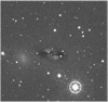 |
Fig. C.1 Residual image produced by the GALFITM of the galaxy NGC 1023 observed in the u band. The FoV is ≈ 0.02 deg2. |
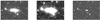 |
Fig. C.2 Illustration of the median smoothing method. Left panel: Original image. Central panel: Median of the original image produced with the MEDIAN tool from the IRAF package. Right panel: Residual image after median subtraction. FoV is ≈ 0.1 deg2. |
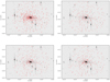 |
Fig. C.3 Comparison of applied methods. Top left panel: GCs present in the reference catalog from Kartha et al. (2014). Top right panel: GCs detected using the Source Extractor method that are also presented in Kartha et al. (2014). Bottom left panel: GCs detected using the median smoothing method that are also found in Kartha et al. (2014). Bottom right panel: Objects detected using ISOFIT and CMODEL method (Ciambur 2015) that are also reported in Kartha et al. (2014). In the background we show the white image of NGC 1023 used for the detection of sources. FoV is ≈ 0.1 deg2. |
Appendix D Color Bimodality Analysis: BIC and ICL Values
Table D.1 shows the BIC and ICL values for GMM with one and two components, following the results presented in Section 4.1.
BIC and ICL values for GMM with one and two components for each color.
References
- Aguilar, L. A., & White, S. D. M. 1985, ApJ, 295, 374 [NASA ADS] [CrossRef] [Google Scholar]
- Aguilar, L. A., & White, S. D. M. 1986, ApJ, 307, 97 [Google Scholar]
- Alabi, A. B., Forbes, D. A., Romanowsky, A. J., et al. 2016, MNRAS, 460, 3838 [Google Scholar]
- Alamo-Martínez, K., & Blakeslee, J. 2017, ApJ, 849, 6 [CrossRef] [Google Scholar]
- Bamford, S. P., Häußler, B., Rojas, A., & Borch, A. 2011, ASP Conf. Ser., 442, 479 [NASA ADS] [Google Scholar]
- Barbon, R., & Capaccioli, M. 1975, A&A, 42, 103 [NASA ADS] [Google Scholar]
- Barden, M., Häußler, B., Peng, C. Y., McIntosh, D. H., & Guo, Y. 2012, Astrophysics Source Code Library [record ascl: 1203.002] [Google Scholar]
- Beasley, M. A. 2020, Globular Cluster Systems and Galaxy Formation (Berlin: Springer), 245 [Google Scholar]
- Beasley, M. A., Bridges, T., Peng, E., et al. 2008, MNRAS, 386, 1443 [NASA ADS] [CrossRef] [Google Scholar]
- Belokurov, V., Erkal, D., Evans, N., Koposov, S., & Deason, A. 2018, MNRAS, 478, 611 [NASA ADS] [CrossRef] [Google Scholar]
- Bender, R., Doebereiner, S., & Moellenhoff, C. 1988, ApJS, 74, 385 [Google Scholar]
- Benitez, N., Dupke, R., Moles, M., et al. 2014, ArXiv e-prints [arXiv:1403.5237] [Google Scholar]
- Berriman, G. B., Deelman, E., Good, J. C., et al. 2004, Proc. Int. Soc. Opt. Eng., 5493, 221 [Google Scholar]
- Bertin, E., & Arnouts, S. 1996, A&AS, 117, 393 [NASA ADS] [CrossRef] [EDP Sciences] [Google Scholar]
- Bílek, M., Samurović, S., & Renaud, F. 2019, A&A, 625, A32 [Google Scholar]
- Binney, J., & Tremaine, S. 2008, Galactic Dynamics, 2nd edn. (Princeton: Princeton University Press) [Google Scholar]
- Blakeslee, J. P., Cho, H., Peng, E. W., et al. 2012, ApJ, 746, 88 [NASA ADS] [CrossRef] [Google Scholar]
- Blom, C., Forbes, D. A., Brodie, J. P., et al. 2012a, MNRAS, 426, 1959 [Google Scholar]
- Blom, C., Spitler, L. R., & Forbes, D. A. 2012b, MNRAS, 420, 37 [Google Scholar]
- Brodie, J. P., & Strader, J. 2006, ARA&A, 44, 193 [Google Scholar]
- Brodie, J. P., Usher, C., Conroy, C., et al. 2012, ApJ, 759, L33 [NASA ADS] [CrossRef] [Google Scholar]
- Brodie, J. P., Romanowsky, A. J., Strader, J., et al. 2014, ApJ, 796, 52 [Google Scholar]
- Bruzual, G., & Charlot, S. 2003, MNRAS, 344, 1000 [NASA ADS] [CrossRef] [Google Scholar]
- Buzzo, M. L., Cortesi, A., Hernandez-Jimenez, J. A., et al. 2021, MNRAS, 504, 2146 [NASA ADS] [CrossRef] [Google Scholar]
- Buzzo, M. L., Cortesi, A., Forbes, D. A., et al. 2022, MNRAS, 510, 1383 [Google Scholar]
- Cantiello, M., & Blakeslee, J. P. 2007, ApJ, 669, 982 [NASA ADS] [CrossRef] [Google Scholar]
- Cantiello, M., Blakeslee, J. P., Raimondo, G., et al. 2014, A&A, 564, L3 [NASA ADS] [CrossRef] [EDP Sciences] [Google Scholar]
- Capaccioli, M., Lorenz, H., & Afanasjev, V.L. 1986, A&A, 169, 54 [NASA ADS] [Google Scholar]
- Cenarro, A. J., Moles, M., Cristóbal-Hornillos, D., et al. 2019, A&A, 622, A176 [NASA ADS] [CrossRef] [EDP Sciences] [Google Scholar]
- Chabrier, G. 2003, PASP, 115, 763 [Google Scholar]
- Chambers, K. C., Magnier, E., Metcalfe, N., et al. 2016, ArXiv e-prints [arXiv:1612.05560] [Google Scholar]
- Chen, Y., Bressan, A., Girardi, L., et al. 2015, MNRAS, 452, 1068 [Google Scholar]
- Chies-Santos, A., Larsen, S., Kuntschner, H., et al. 2011, A&A, 525, A20 [NASA ADS] [CrossRef] [EDP Sciences] [Google Scholar]
- Chies-Santos, A. L., Cortesi, A., Fantin, D. S. M., et al. 2013, A&A, 559, A67 [NASA ADS] [CrossRef] [EDP Sciences] [Google Scholar]
- Chies-Santos, A. L., de Souza, R. S., Caso, J. P., et al. 2022, MNRAS, accepted [arXiv:2202.11472] [Google Scholar]
- Cho, H., Blakeslee, J. P., Chies-Santos, A. L., et al. 2016, ApJ, 822, 95 [NASA ADS] [CrossRef] [Google Scholar]
- Choksi, N., & Gnedin, O. Y. 2019, MNRAS, 486, 331 [NASA ADS] [CrossRef] [Google Scholar]
- Choksi, N., Gnedin, O. Y., & Li, H. 2018, MNRAS, 480, 2343 [NASA ADS] [CrossRef] [Google Scholar]
- Chung, C., Yoon, S.-J., Lee, S.-Y., & Lee, Y.-W. 2016, ApJ, 818, 201 [NASA ADS] [CrossRef] [Google Scholar]
- Ciambur, B. C. 2015, ApJ, 810, 120 [NASA ADS] [CrossRef] [Google Scholar]
- Cid Fernandes, R., Pérez, E., García Benito, R., et al. 2013, A&A, 557, A86 [NASA ADS] [CrossRef] [EDP Sciences] [Google Scholar]
- Coe, D., Umetsu, K., Zitrin, A., et al. 2012, ApJ, 757, 22 [NASA ADS] [CrossRef] [Google Scholar]
- Combes, F., Rampazzo, R., Bonfanti, P. P., Prugniel, P., & Sulentic, J. W. 1995, A&A, 297, 37 [NASA ADS] [Google Scholar]
- Cortesi, A., Merrifield, M., & Arnaboldi, M. 2011, Astrophys. Space Sci. Proc., 27, 109 [NASA ADS] [CrossRef] [Google Scholar]
- Cortesi, A., Chies-Santos, A. L., Pota, V., et al. 2016, MNRAS, 456, 2611 [NASA ADS] [CrossRef] [Google Scholar]
- Costa-Duarte, M., Sampedro, L., Molino, A., et al. 2019, MNRAS, submitted [arXiv: 1909.08626] [Google Scholar]
- Cristóbal-Hornillos, D., Varela, J., Ederoclite, A., et al. 2014, Proc. SPIE, 9152, 91520O [CrossRef] [Google Scholar]
- Das, P., Hawkins, K., & Jofré, P. 2020, MNRAS, 493, 5195 [NASA ADS] [CrossRef] [Google Scholar]
- Davoust, E., & Prugniel, P. 1988, A&A, 201, L30 [NASA ADS] [Google Scholar]
- Debattista, V. P., Corsini, E. M., & Aguerri, J. A. L. 2002, MNRAS, 332, 65 [Google Scholar]
- De Souza, R., Dantas, M., Costa-Duarte, M., et al. 2017, MNRAS, 472, 2808 [NASA ADS] [CrossRef] [Google Scholar]
- Dolfi, A., Forbes, D. A., Couch, W. J., et al. 2021, MNRAS, 504, 4923 [NASA ADS] [CrossRef] [Google Scholar]
- Eadie, G. M., Harris, W. E., & Springford, A. 2022, ApJ, 926, 162 [NASA ADS] [CrossRef] [Google Scholar]
- Elmegreen, B. G. 2000, in Toward a New Millennium in Galaxy Morphology (Berlin: Springer), 469 [CrossRef] [Google Scholar]
- Fahrion, K., Lyubenova, M., Hilker, M., et al. 2020, A&A, 637, A27 [NASA ADS] [CrossRef] [EDP Sciences] [Google Scholar]
- Falcón-Barroso, J., Sánchez-Blázquez, P., Vazdekis, A., et al. 2011, A&A, 532, A95 [Google Scholar]
- Finlator, K., Ivezić, Ž., Fan, X., et al. 2000, ApJ, 120, 2615 [CrossRef] [Google Scholar]
- Forbes, D. A., Almeida, A., Spitler, L. R., & Pota, V. 2014, MNRAS, 442, 1049 [NASA ADS] [CrossRef] [Google Scholar]
- Forbes, D. A., Romanowsky, A. J., Pastorello, N., et al. 2016, MNRAS, 457, 1242 [NASA ADS] [CrossRef] [Google Scholar]
- Gaia Collaboration (Brown, A.G.A., et al.) 2016a, A&A, 595, A2 [NASA ADS] [CrossRef] [EDP Sciences] [Google Scholar]
- Gaia Collaboration (Prusti, T., et al.) 2016b, A&A, 595, A1 [NASA ADS] [CrossRef] [EDP Sciences] [Google Scholar]
- Gaia Collaboration (Brown, A., et al.) 2018, A&A, 616, A1 [NASA ADS] [CrossRef] [EDP Sciences] [Google Scholar]
- Gaia Collaboration (Brown, A., et al.) 2021, A&A, 649, A1 [NASA ADS] [CrossRef] [EDP Sciences] [Google Scholar]
- González-Serrano, J. I., & Carballo, R. 2000, A&AS, 142, 353 [NASA ADS] [CrossRef] [EDP Sciences] [Google Scholar]
- González Delgado, R. M., Díaz-García, L. A., de Amorim, A., et al. 2021, A&A, 649, A79 [Google Scholar]
- Goto, T., Sekiguchi, M., Nichol, R.C., et al. 2002, AJ, 123, 1807 [NASA ADS] [CrossRef] [Google Scholar]
- Harris, W. E. 2001, in Star Clusters (Berlin: Springer), 223 [NASA ADS] [CrossRef] [Google Scholar]
- Hart, L., Davies, R. D., & Johnson, S. C. 1980, MNRAS, 191, 269 [NASA ADS] [CrossRef] [Google Scholar]
- Häußler, B., Bamford, S. P., Vika, M., et al. 2013, MNRAS, 430, 330 [Google Scholar]
- Helmi, A., Babusiaux, C., Koppelman, H. H., et al. 2018, Nature, 563, 85 [Google Scholar]
- Horta, D., Schiavon, R. P., Mackereth, J. T., et al. 2021, MNRAS, 500, 1385 [Google Scholar]
- Ivezić, Ž., Connolly, A. J., VanderPlas, J. T., & Gray, A. 2014, Statistics, Data Mmining, and Machine Learning in Astronomy (Princeton: Princeton University Press) [CrossRef] [Google Scholar]
- Jedrzejewski, R. I. 1987, MNRAS, 226, 747 [Google Scholar]
- Kartha, S. S., Forbes, D. A., Spitler, L. R., et al. 2014, MNRAS, 437, 273 [NASA ADS] [CrossRef] [Google Scholar]
- Kim, S., Yoon, S.-J., Lee, S.-Y., Chung, C., & Sohn, S. T. 2021, ApJS, 256, 29 [NASA ADS] [CrossRef] [Google Scholar]
- Koppelman, H. H., Helmi, A., Massari, D., Price-Whelan, A. M., & Starkenburg, T. K. 2019, A&A, 631, L9 [NASA ADS] [CrossRef] [EDP Sciences] [Google Scholar]
- Kruijssen, J. D., Pfeffer, J. L., Crain, R. A., & Bastian, N. 2019a, MNRAS, 486, 3134 [NASA ADS] [CrossRef] [Google Scholar]
- Kruijssen, J. D., Pfeffer, J. L., Reina-Campos, M., Crain, R. A., & Bastian, N. 2019b, MNRAS, 486, 3180 [NASA ADS] [CrossRef] [Google Scholar]
- Kruijssen, J. D., Pfeffer, J. L., Chevance, M., et al. 2020, MNRAS, 498, 2472 [NASA ADS] [CrossRef] [Google Scholar]
- Kundu, A., & Whitmore, B. C. 1998, AJ, 116, 2841 [NASA ADS] [CrossRef] [Google Scholar]
- Kundu, A., & Zepf, S. E. 2007, ApJ, 660, L109 [NASA ADS] [CrossRef] [Google Scholar]
- Larsen, S. S. 2001, AJ, 122, 1782 [NASA ADS] [CrossRef] [Google Scholar]
- Larsen, S. S., Brodie, J. P., Huchra, J. P., Forbes, D. A., & Grillmair, C. J. 2001, AJ, 121, 2974 [NASA ADS] [CrossRef] [Google Scholar]
- Lauer, T. R. 1986, ApJ, 311, 34 [NASA ADS] [CrossRef] [Google Scholar]
- Lauer, T. R. 1988, ApJ, 325, 49 [NASA ADS] [CrossRef] [Google Scholar]
- Lawson, C. L., & Hanson, R. J. 1974, Solving Least Squares Problems (Englewood Cliffs, New Jersey: Prentice-Hall, Inc.) [Google Scholar]
- Lee, S.-Y., Chung, C., & Yoon, S.-J. 2018, ApJS, 240, 2 [CrossRef] [Google Scholar]
- Lee, S.-Y., Chung, C., & Yoon, S.-J. 2020, ApJ, 905, 124 [NASA ADS] [CrossRef] [Google Scholar]
- Lenzen, R., Hartung, M., Brandner, W., et al. 2003, SPIE, 4841, 944 [Google Scholar]
- Li, H., & Gnedin, O. 2019, Proc. Int. Astron. Union, 14, 34 [CrossRef] [Google Scholar]
- Li, H., & Gnedin, O. Y. 2014, ApJ, 796, 10 [Google Scholar]
- López-Sanjuan, C., Ramió, H. V., Varela, J., et al. 2019, A&A, 622, A177 [NASA ADS] [CrossRef] [EDP Sciences] [Google Scholar]
- Lotz, J. M., Miller, B. W., & Ferguson, H. C. 2004, ApJ, 613, 262 [NASA ADS] [CrossRef] [Google Scholar]
- Magris C.G., Mateu P.J., Mateu, C., et al. 2015, PASP, 127, 16 [NASA ADS] [CrossRef] [Google Scholar]
- Marigo, P., Bressan, A., Nanni, A., Girardi, L., & Pumo, M. L. 2013, MNRAS, 434, 488 [Google Scholar]
- Marín-Franch, A., Taylor, K., Cenarro, J., Cristobal-Hornillos, D., & Moles, M. 2015, IAU General Assembly, 29, 2257381 [Google Scholar]
- Mejía-Narváez, A., Bruzual, G., Magris, C. G., et al. 2017, MNRAS, 471, 4722 [Google Scholar]
- Mendes de Oliveira, C., Ribeiro, T., Schoenell, W., et al. 2019, MNRAS, 489, 241 [NASA ADS] [CrossRef] [Google Scholar]
- Möllenhoff, C., & Heidt, J. 2001, A&A, 368, 16 [NASA ADS] [CrossRef] [EDP Sciences] [Google Scholar]
- Mora, M. D., Torres-Flores, S., Firpo, V., et al. 2019, MNRAS, 488, 830 [NASA ADS] [CrossRef] [Google Scholar]
- Morganti, R., de Zeeuw, P. T., Oosterloo, T. A., et al. 2006, MNRAS, 371, 157 [Google Scholar]
- Muratov, A. L., & Gnedin, O. Y. 2010, ApJ, 718, 1266 [Google Scholar]
- Myeong, G., Vasiliev, E., Iorio, G., Evans, N., & Belokurov, V. 2019, MNRAS, 488, 1 [Google Scholar]
- Nakazono, L., de Oliveira, C. M., Hirata, N., et al. 2021, MNRAS, 507, 5847 [CrossRef] [Google Scholar]
- Noordermeer, E., Merrifield, M. R., Coccato, L., et al. 2008, MNRAS, 384, 943 [NASA ADS] [CrossRef] [Google Scholar]
- Pedregosa, F., Varoquaux, G., Gramfort, A., et al. 2011, J. Mach. Lear. Res., 12, 2825 [Google Scholar]
- Peng, C. Y., Ho, L. C., Impey, C. D., & Rix, H.-W. 2002, AJ, 124, 266 [Google Scholar]
- Peng, E. W., Jordán, A., Côté, P., et al. 2006, ApJ, 639, 95 [Google Scholar]
- Pfeffer, J., Kruijssen, J. D., Crain, R. A., & Bastian, N. 2018, MNRAS, 475, 4309 [NASA ADS] [CrossRef] [Google Scholar]
- Phillipps, S., Drinkwater, M., Gregg, M., & Jones, J. 2001, ApJ, 560, 201 [NASA ADS] [CrossRef] [Google Scholar]
- Plat, A., Charlot, S., Bruzual, G., et al. 2019, MNRAS, 490, 978 [Google Scholar]
- Prakash, A., Licquia, T. C., Newman, J. A., & Rao, S. M. 2015, ApJ, 803, 105 [NASA ADS] [CrossRef] [Google Scholar]
- Prugniel, P., Vauglin, I., & Koleva, M. 2011, A&A, 531, A165 [NASA ADS] [CrossRef] [EDP Sciences] [Google Scholar]
- Puzia, T. H., Zepf, S. E., Kissler-Patig, M., et al. 2002, A&A, 391, 453 [NASA ADS] [CrossRef] [EDP Sciences] [Google Scholar]
- Richtler, T. 2005, Bulletin of the Astronomical Society of India, 34, 83 [NASA ADS] [Google Scholar]
- Romanowsky, A. J., Strader, J., Brodie, J. P., et al. 2012, ApJ, 748, 29 [Google Scholar]
- Sánchez-Blázquez, P., Peletier, R. F., Jiménez-Vicente, J., et al. 2006, MNRAS, 371, 703 [Google Scholar]
- Sancisi, R., van Woerden, H., Davies, R. D., & Hart, L. 1984, MNRAS, 210, 497 [NASA ADS] [CrossRef] [Google Scholar]
- Schlafly, E. F., & Finkbeiner, D. P. 2011, ApJ, 737, 103 [Google Scholar]
- Sharma, K., Prugniel, P., & Singh, H. P. 2016, A&A, 585, A64 [NASA ADS] [CrossRef] [EDP Sciences] [Google Scholar]
- Strader, J., Brodie, J. P., Cenarro, A., Beasley, M. A., & Forbes, D. A. 2005, AJ, 130, 1315 [NASA ADS] [CrossRef] [Google Scholar]
- Strauss, M. A., Weinberg, D. H., Lupton, R. H., et al. 2002, AJ, 124, 1810 [Google Scholar]
- Taylor, M. B. 2006, ASP Conf. Ser., 351, 666 [Google Scholar]
- Tody, D. 1993, ASP Conf. Ser., 52, 173 [NASA ADS] [Google Scholar]
- Tully, R. B. 1980, ApJ, 237, 390 [NASA ADS] [CrossRef] [Google Scholar]
- Usher, C., Forbes, D. A., Brodie, J. P., et al. 2012, MNRAS, 426, 1475 [Google Scholar]
- Valdes, F., Gupta, R., Rose, J. A., Singh, H. P., & Bell, D. J. 2004, ApJS, 152, 251 [Google Scholar]
- Varela, J., d’Onofrio, M., Marmo, C., et al. 2009, A&A, 497, 667 [NASA ADS] [CrossRef] [EDP Sciences] [Google Scholar]
- Villaume, A., Romanowsky, A. J., Brodie, J., & Strader, J. 2019, ApJ, 879, 45 [NASA ADS] [CrossRef] [Google Scholar]
- Wang, C., Bai, Y., Yuan, H., Wang, S., & Liu, J. 2021, A&A, 659, A144 [Google Scholar]
- Yong, D., Norris, J. E., Bessell, M. S., et al. 2012, ApJ, 762, 26 [Google Scholar]
- Yoon, S.-J., Yi, S. K., & Lee, Y.-W. 2006, Science, 311, 1129 [Google Scholar]
- Yoon, S.-J., Lee, S.-Y., Blakeslee, J. P., et al. 2011, ApJ, 743, 150 [NASA ADS] [CrossRef] [Google Scholar]
- York, D. G., Adelman, J., Anderson Jr, J. E., et al. 2000, AJ, 120, 1579 [NASA ADS] [CrossRef] [Google Scholar]
All Tables
Number of GC candidates selected per band after the selection criteria are applied.
Precision (mean standard deviation) of the stellar population properties derived with the TGASPEX code.
All Figures
|
Fig. 1 J-PLUS color image of NGC 1023 obtained with the software Trilogy (Coe et al. 2012). To build the color image, the combination of filters (u, J0378, J0410), (J0430, J0515, g), and (J0660, J0861, r, i, z) were used to compose the blue, green, and red components, respectively. The FoV is ≈ 0.1 deg2. |
| In the text | |
|
Fig. 2 Spatial distribution of GC candidates. In the background we show the white image of NGC 1023 used for the detection of sources. The FoV is ≈0.1 deg2. Red circles represent GC candidates from the reference catalog (Kartha et al. 2014). Blue circles represent GCs in common between GCFinder selection and the reference catalog. |
| In the text | |
|
Fig. 3 Examples of SED fitting for 3 GC candidates. The observed and synthetic SEDs are presented in black and blue, respectively. The model fits of the two codes are very similar, therefore, they appear superposed in the figure. |
| In the text | |
|
Fig. 4 Color distribution computed using broad-band filters only. The curves represent the unimodal (black) and bimodal (purple) distributions returned by the GMM analysis. We also show in blue and red dashed lines the two peaks that compose the bimodal distribution. BICs values for GMM with one and two components are shown as an example. |
| In the text | |
|
Fig. 5 Color distribution computed using narrow–band filters only. The curves represent the unimodal (black) and bimodal (purple) distributions returned by the GMM analysis. We also show in blue and red the two peaks that compose the bimodal distribution. The BIC values for GMM with one and two components are shown as an example. |
| In the text | |
|
Fig. 6 Distribution of stellar masses obtained from SED fitting. The left panel illustrates the results from DynBaS 3, while the right panel shows the results from TGASPEX. The distributions display a broad peak with log Stellar Masses between 5 and 6 M⊙. In red, we show the results obtained using all available filters. Green represents results obtained using broadband filters only. Blue represents results obtained using narrowband filters only. |
| In the text | |
|
Fig. 7 Distribution of logarithmic ages obtained from SED fitting. Upper and lower panels illustrate results from DynBaS 3 and TGASPEX respectively. Left and right panels: results for mass- and light-weighted ages, respectively. Red represents results obtained using all available filters. Green represents results obtained using broadband filters only. Blue represents results obtained using narrowband filters only. |
| In the text | |
|
Fig. 8 Distribution of metallicities obtained from SED fitting. Upper and lower panels: illustrate results for DynBaS 3 and TGASPEX respectively. Left and right panels: results for mass- and light-weighted Z, respectively. Red represents results obtained using all available filters. Green represents results obtained using broadband filters only. Blue represents results obtained using narrowband filters only. |
| In the text | |
|
Fig. 9 Correlation between ages and masses derived via SED fitting. A trend where the mean ages of the cluster-candidates increase with stellar masses is seen for all combinations of code and filter set. Left and right panels: illustrate the results for DynBaS 3 and TGASPEX, respectively. Red triangles represent results obtained using all bands, green circles represent results when using only the broadband, and blue stars represent results obtained from the narrowband only. |
| In the text | |
|
Fig. 10 AMR for the NGC 1023 GC system based on DynBaS 3 (blue circles) compared to 3 E-MOSAIC simulations: MW014, MW016, and MW023 from Kruijssen et al. (2019a) (grey contours) that have comparable halo masses to NGC 1023. We observe a (likely) broad AMR of NGC 1023 GC system, where the objects have a broad metallicity distribution and are mainly old. |
| In the text | |
|
Fig. 11 Displaced nucleus of NGC 1023. Top panel: offset radius profile with respect to the photometric center of the galaxy. Bottom panel: selected outer isophotes (in black) with their respective fitted ellipses (blue) are overplotted on r-band image. The blue pluses are their respective centers, while the red point is the photometric center of the galaxy, and the green point is the photometric center of GCs candidates. The top-right inset is a zoom-in of the inner part to better see the displacements. The blue points in the offset radius profile are the offsets for the selected isophotes. |
| In the text | |
|
Fig. 12 Photometric model for NGC 1023. Left panel: R-band image. Middle panel: ellipse model. Right panel: residual map, with NGC 1023A revealed, together with two spiral arms and an inner bar. |
| In the text | |
|
Fig. A.1 Illustration of the Source Extractor method. Left panel: Zoom on the NGC 1023 image. Right panel: Illustration of the way Source Extractor interprets the image with the chosen input parameters. |
| In the text | |
|
Fig. A.2 Illustration of the selection by quality and shape (phase 1). Top panel: Magnitude error as function of the source magnitude. Bottom panel: FWHM of the sources as a function of the source magnitude. Objects in the gray area have been discarded, following the selection criteria described in the text. |
| In the text | |
|
Fig. A.3 Illustration of the selection by color (phase 2). Top panel: Selection of the GC candidates on the color-color diagram of the detections. Objects in the gray area have been discarded. A red line was included to guide the eye. Bottom panel: same as top panel with GC candidates also presented in Kartha et al. (2014) in magenta. |
| In the text | |
|
Fig. A.4 Adopted upper limit in terms of magnitude (phase 3). Objects in the gray area have been discarded. |
| In the text | |
|
Fig. A.5 Distribution of parallaxes for the GC candidates as obtained from Gaia EDR3. The blue distribution corresponds to the candidates of the present wok and magenta shows the distribution of GC candidates identified by Kartha et al. (2014). |
| In the text | |
|
Fig. A.6 Density distributions of colors based on J-PLUS filters. Magenta: Color distribution of GC candidates identified by GCFinder that are also present in the reference catalog (Kartha et al. 2014). Grey: Color distribution of GC candidates identified by GCFinder that are not present in the reference cátalos. |
| In the text | |
|
Fig. C.1 Residual image produced by the GALFITM of the galaxy NGC 1023 observed in the u band. The FoV is ≈ 0.02 deg2. |
| In the text | |
|
Fig. C.2 Illustration of the median smoothing method. Left panel: Original image. Central panel: Median of the original image produced with the MEDIAN tool from the IRAF package. Right panel: Residual image after median subtraction. FoV is ≈ 0.1 deg2. |
| In the text | |
|
Fig. C.3 Comparison of applied methods. Top left panel: GCs present in the reference catalog from Kartha et al. (2014). Top right panel: GCs detected using the Source Extractor method that are also presented in Kartha et al. (2014). Bottom left panel: GCs detected using the median smoothing method that are also found in Kartha et al. (2014). Bottom right panel: Objects detected using ISOFIT and CMODEL method (Ciambur 2015) that are also reported in Kartha et al. (2014). In the background we show the white image of NGC 1023 used for the detection of sources. FoV is ≈ 0.1 deg2. |
| In the text | |
Current usage metrics show cumulative count of Article Views (full-text article views including HTML views, PDF and ePub downloads, according to the available data) and Abstracts Views on Vision4Press platform.
Data correspond to usage on the plateform after 2015. The current usage metrics is available 48-96 hours after online publication and is updated daily on week days.
Initial download of the metrics may take a while.