| Issue |
A&A
Volume 691, November 2024
|
|
|---|---|---|
| Article Number | A144 | |
| Number of page(s) | 13 | |
| Section | Galactic structure, stellar clusters and populations | |
| DOI | https://doi.org/10.1051/0004-6361/202451059 | |
| Published online | 08 November 2024 | |
Determination of metallicities of red giant stars using machine learning techniques applied to the narrow and broadband photometry of the S-PLUS survey
1
Departamento de Astronomía, Universidad de La Serena,
Av. J. Cisternas 1200 N,
1720236
La Serena,
Chile
2
Cerro Tololo Inter-American Observatory/NSF’s NOIRLab,
Casilla 603,
La Serena,
Chile
3
Instituto Multidisciplinario de Investigación y Postgrado, Universidad de La Serena,
Av. R. Bitrán 1305,
1720256
La Serena,
Chile
4
Departamento de Astronomia, Instituto de Astronomia, Geofísica e Ciências Atmosféricas da USP, Cidade Universitária,
05508-900
São Paulo,
SP,
Brazil
5
NSF’s NOIRLab,
950 N. Cherry Ave.,
Tucson,
AZ
85719,
USA
6
Observatório Nacional, Ministério da Ciência, Tecnologia,
Inovação e Comunicações,
Brazil
7
GMTO Corporation
465 N. Halstead Street, Suite 250
Pasadena,
CA
91107,
USA
8
Rubin Observatory Project Office,
950 N. Cherry Ave.,
Tucson,
AZ
85719,
USA
9
Departamento de Física, Universidade Federal de Santa Catarina,
Florianópolis,
SC
88040-900,
Brazil
★ Corresponding author; This email address is being protected from spambots. You need JavaScript enabled to view it.
Received:
11
June
2024
Accepted:
7
August
2024
Abstract
Aims. The aim of this study is to obtain metallicities of red giant stars from the Southern Photometric Local Universe Survey (S-PLUS) and to classify giant and dwarf stars using artificial neural networks applied to the S-PLUS photometry.
Methods. We combined the five broadband and seven narrow-band filters of S-PLUS – especially centred on prominent stellar spectral features – to train machine learning algorithms. The training catalogue was made by cross-matching the S-PLUS and Apache Point Observatory Galactic Evolution Experiment 2 (APOGEE-2) survey catalogues. The classification neural network uses the colours (J0378 - u), (J0395 - g), (J0410 - g), (J0515 - g), (J0660 - r), (g - z) and (r - i) as input features, whereas the network for metallicities uses the colours (J0378 - u), (J0395 - g), (J0410 - g), (J0515 - g), (J0660 - r), (u - g) and (r - z) as input features.
Results. The resulting network is capable of identifying ~99% of the giants in the test set. The network for determining the photometric metallicities of giant stars estimates metallicities in the test set a with a standard deviation of σgiants ~ 0.07 dex with respect to the spectroscopic values. Finally, we used the trained artificial neural networks to generate a publicly available catalogue of 523 426 stars classified as red giant stars from S-PLUS, which we used to explore metallicity gradients in the Milky Way.
Key words: methods: data analysis / catalogs / stars: abundances / stars: late-type
© The Authors 2024
 Open Access article, published by EDP Sciences, under the terms of the Creative Commons Attribution License (https://creativecommons.org/licenses/by/4.0), which permits unrestricted use, distribution, and reproduction in any medium, provided the original work is properly cited.
This article is published in open access under the Subscribe to Open model. This email address is being protected from spambots. You need JavaScript enabled to view it. to support open access publication.
1 Introduction
The study of substructures in the Milky Way provides important clues to understanding the formation of the Galaxy in a cosmological context. To do this, it is crucial to have tracers easily distinguished within their environment (Vivas & Zinn 2002). Among these tracers, red giant stars offer great potential to study substructures in the Galaxy, especially in the halo, and even at greater distances within the Local Group (Grunblatt et al. 2021; James et al. 2021). This is doable because red giant stars are numerous enough to trace substructures and bright enough to be detected at great distances, unlike dwarf stars, which are numerous but intrinsically faint. Additionally, K-type giant stars are found in populations of all ages and metallicities, so any substructure is potentially traceable by this type of star (Majewski 2004).
Traditionally, the study of Galaxy components is generally carried out by identifying their individual stars’ dynamic and chemical properties (Eggen et al. 1962). In this sense, the chemical properties of stars are first determined using their global metallicity. The determination of metallicity is not easy. On the one hand, they can be obtained with high accuracy through spectroscopy, however, this comes at the expense of telescope time, even with current multiplexed surveys. On the other hand, applying photometric methods for the same purposes presents an opportunity due to the large number of stars that can be observed simultaneously; all the stars in the field of view. However, the precision of resulting metallicities is lower than their spectroscopic counterpart, reaching uncertainties of ~0.2 dex in metallicity (Ivezić et al. 2008; Gu et al. 2015; Casagrande et al. 2019; Chiti et al. 2021).
A more approachable method of determining stellar metallicities is using photometric indices. These photometric indices measure the flux from the spectral region of a line by photometry with a narrow-band filter. The intensity of the line is estimated by comparing the intensity of the continuum spectrum (calculated by photometry with a broadband filter). Subsequently, indices are calibrated using stars with stellar parameters known using spectra and applied to the sample to be studied (e.g. Geisler 1986). Although the precision of the photometric methods is lower, this is compensated for by the large number of objects that can be studied simultaneously, and the accuracy is enough to carry out various studies.
The arrival of large surveys during the last decades has provided us with large volumes of data. These surveys are relevant in terms of extensive sky coverage and are equipped with several bandpasses collected in a homogeneous and digitised fashion. An example of this is the Sloan Digital Sky Survey (SDSS; York et al. 2000), which provides large photometric catalogues readily available online. Other examples of this kind of survey are: the Two Micron All-Sky Survey (2MASS; Skrutskie et al. 2006), VISTA Hemisphere Survey (VHS; McMahon et al. 2013), Panoramic Survey Telescope and Rapid Response System (Pan-STARRS; Chambers et al. 2016), Dark Energy Survey (DES; Dark Energy Survey Collaboration 2016), and SkyMapper (Wolf et al. 2018). The previous examples correspond to surveys comprising broadband filters within the 3000–10 000 Å or the near-infrared (near-IR) bands, which make them sensitive mainly to the characteristics of the continuum; that is, the effective temperature. The need to obtain photometric information sensitive to stellar metallicity has triggered the advent of large-area surveys that utilise narrow-band filters centred on relevant spectral features. When combined with broadband filters, such photometric colours are sensitive to the intensity of the spectral lines. Some examples of such surveys are the Javalambre Photometric Local Universe Survey (J-PLUS; Cenarro et al. 2019) and the Southern Photometric Local Universe Survey (S-PLUS; Mendes de Oliveira et al. 2019).
Javalambre’s photometric system covers the optical range and part of the near-IR (between 3500 and 10 000 Å) and is composed of a combination of five broadband filters and seven narrow-band filters (Cenarro et al. 2019). The five broadband filters correspond to the ugriz filters, the last four similar to those of SDSS (Fukugita et al. 1996), and the u filter is specially designed for the Javalambre system, with greater efficiency than the u band of SDSS (Mendes de Oliveira et al. 2019). The seven narrow-band filters (J0378, J0395, J0410, J0430, J0515, J0660, and J0861) are located on prominent spectral features. These features provide an ideal setting for classifying and characterising stellar populations (Cenarro et al. 2019). This photometric system is optimised for stellar classification and determining the stellar parameters: effective temperature (Teff), surface gravity (log g) and metallicity ([M/H]) (Gruel et al. 2012; Marín-Franch et al. 2012; Whitten et al. 2019; Galarza et al. 2022). The different parameters of the stellar atmosphere imply a variation in the equivalent width of a spectral line (a variation of the flux in the region of the line), and therefore in the photometric bandpass (see e.g. Fig. 3 of Dias et al. 2015, Fig. 2 of Dias et al. 2017). For example, the dependence of the magnesium triplet on the stellar surface gravity has long been known (Öhman 1934; Thackeray 1939). Some studies have shown the dependence between the lines of the calcium triplet and the metallicity of red giants in star clusters (Armandroff & Da Costa 1991; Cole et al. 2004; Warren & Cole 2009; Dias & Parisi 2020). The complexity of the relationships between the stellar parameters and the spectral features makes machine learning an excellent tool to address this problem.
Machine learning is ‘the field of study that allows computers to learn without being explicitly programmed’ (Samuel 2000). Mitchell (1997) defined machine learning as ‘the study of computer algorithms that improve automatically through experience’. Machine learning is beneficial and practical for solving problems whose solutions can be very complex or very demanding in time. It is also helpful to obtain information from large amounts of data (for a more complex insight into machine learning techniques, see Géron 2017). Artificial neural networks (ANNs), commonly referred to as neural networks (NNs), are a model based on the biological NNs that constitute the nervous system of animals (Sammut & Webb 2010). Deep learning is an area within machine learning that is essentially based on deep neural networks (DNNs) (with three or more layers) (IBM Cloud Education 2020).
The development of deep learning and ANNs in recent decades has been strengthened mainly by the large amount of data available to train them and by the improvement in the capabilities of computers from the 1990s to the present (Géron 2017). Currently, machine learning and deep learning technologies drive many aspects of modern society: speech recognition (e.g. Apple Siri, Amazon Alexa, Microsoft Cortana, Google Now), language processing (e.g. Google Translate), content recommendation systems (e.g. Spotify, Netflix, Twitter, Instagram), products or services (e.g. advertisements) of interest of the user, facial recognition (e.g. Facebook), driving assistants (e.g. Google Maps, Uber), self-driving vehicles (e.g. Tesla), drug discovery and toxicology, bioinformatics, image analysis and medical diagnostics, detection of financial fraud, and many additional applications (LeCun et al. 2015; Balas et al. 2019).
Nowadays, astronomical datasets are experiencing a rapid increase in size and complexity, introducing astronomy in the era of big data. Given this rapid growth, astronomers have begun using automated tools to detect, classify, characterise, and analyse objects or sets of astronomical objects. Automated algorithms have been growing in popularity over the last few years of astronomy and have already been implemented in various tasks (Baron 2019). Some examples of studies carried out with deep learning techniques that include the implementation of NNs in astronomy are Yip et al. (2019) in the detection of exoplanets, Soumagnac et al. (2015) in the separation between stars and galaxies, Walmsley et al. (2020) in the classification of galaxies with Bayesian NNs, Lochner et al. (2016) and Mahabal et al. (2017) in the photometric classification of supernovae and light curves, respectively, Das & Sanders (2019) in obtaining distances, masses, and ages from the spectroscopy of red giant stars, Bilicki et al. (2018) in the determination of redshifts, the cosmological study using convolutional NNs of Fluri et al. (2019), and the classification of symbiotic stars (Akras et al. 2019b) and planetary nebulae (Akras et al. 2019a) using machine learning techniques.
In recent years, machine learning techniques have been implemented to determine stellar metallicities employing photometric indices. For example, Miller (2015) developed a method of assessing stellar metallicities from the ugriz filters of SDSS through different machine learning algorithms (K-nearest neighbours, random forest and support vector machines). This method determined the metallicity of stars with a mean square error of 0.29 dex with the spectroscopic measurements. In another contribution, Thomas et al. (2019) presented an algorithm that, from the photometric information of the Canada-France Imaging Survey (CFIS), Pan-STARRS 1 (PS1) and Gaia, is capable of discriminating between dwarf and giant stars and determining their distances and metallicities. The algorithm developed manages to identify more than 70% of the giant stars in the training set, and metallicity estimates have uncertainties of 0.2 dex for [Fe/H] < −1.2. Whitten et al. (2019), for their part, developed a methodology to determine the stellar parameters Teff, log g, and [Fe/H] through NNs from the photometry of the J-PLUS survey, with a particular emphasis on low-metallicity stars. Estimates of the metallicities and temperatures of stars by this method have a 0.25 dex and 91 K dispersion, respectively. Whitten et al. (2021) expanded his approach to main-sequence turn-off K-dwarfs stars from S-PLUS DR2 to estimate the effective temperature, metallicity, and carbonicity. Yang et al. (2022), using photometric data from J-PLUS DR1, Gaia DR2, and spectroscopic labels from the Large sky Area Multi-Object fibre Spectroscopic Telescope, trained a set of cost-sensitive NNs able to determine effective temperature, surface gravity, metallicity, [Fe/H], [α/Fe], and four elemental abundances with a precision of ~0.07 dex for metallicities. Wang et al. (2022) constructed a support vector regression algorithm to estimate the stellar parameters of the stars of J-PLUS with a root mean square error of 0.25 in the metallicities. Galarza et al. (2022) with a series of machine learning models derived the stellar parameters of J-PLUS stars, obtaining an average difference with respect to the spectroscopic values of Δ[Fe/H] ~ 0.09 dex. Huang et al. (2022) determined the biggest amount of metallicities using the photometry of the SkyMapper Southern Survey and Gaia, reaching metallicity values of up to [Fe/H] ~−3.5.
In this work, we have developed a tool capable of deriving the metallicities of red giant stars by training a deep learning algorithm, using S-PLUS photometry, which in turn should classify the stars according to a surface gravity between giant and dwarf stars. The focus on red giant stars allows us to use the results of this work to trace substructures in the Galaxy.
The paper is organised as follows. The dataset and the sample used in this work are described in Section 2. Section 3 explains the architecture of the ANNs. The discrimination process between dwarf and giant stars and the determination of metallicity of red giant stars are described in Sections 4 and 5, respectively. Section 6 shows the results of the application of the ANNs to the complete S-PLUS catalogue. Concluding remarks are given in Section 7.
2 Data
In this work, two datasets were used. The first is the Training, Validation, and Testing catalogue (hereafter, TVT catalogue), which includes the photometric and spectroscopic information for stars in common from S-PLUS and Apache Point Observatory Galactic Evolution Experiment 2 (APOGEE-2), respectively. The second one is the complete catalogue of S-PLUS stars after applying specific quality cuts.
2.1 S-PLUS photometry
The Southern Photometric Local Universe Survey (Mendes de Oliveira et al. 2019) is an ongoing optical photometric survey that began its operations in 2016 and will cover a total area of ~9300 deg2 with the Javalambre’s photometric system (Cenarro et al. 2019). The transmission curves and the characteristics of each filter are shown in Figure 1 and Table 1, respectively. It uses the dedicated robotic telescope T80-South with a 0.826 m aperture and a Ritchey-Chretien configuration, located at the Cerro Tololo Inter-american Observatory (CTIO) in northern Chile. It has a CCD camera of 9232 × 9216 pixels of 10 μm and a scale of 0.55 arcsec/pix, resulting in a 1.4 × 1.4 deg field of view (Mendes de Oliveira et al. 2019; Almeida-Fernandes et al. 2022). The filter system, the telescope, and the camera are identical to those used in the Javalambre Photometric Local Universe Survey (J-PLUS), carried out with the Javalambre Auxiliary Survey Telescope (T80/JAST) at the Javalambre Astrophysical Observatory (OAJ) in Spain (Cenarro et al. 2019). This makes S-PLUS a complementary survey to J-PLUS in the southern hemisphere. S-PLUS has the largest number of photometric bands among the great photometric surveys in the southern hemisphere (Almeida-Fernandes et al. 2022).
In this work, we have used the photometric catalogues of S-PLUS Data Release 3 (S-PLUS DR3, Buzzo et al., in prep.). The S-PLUS DR3 has over 50 million detections (Almeida-Fernandes 2020). The DR3 catalogues cover an area of the sky corresponding to 2214 deg2 distributed in 1107 fields. We used the PSTotal magnitudes from a 3 arcseconds fixed circular aperture, with aperture correction, because they better represent the total magnitude of the point sources (Almeida-Fernandes et al. 2022).
We obtained de-reddened S-PLUS magnitudes that are corrected by interstellar extinction, as follows:
![Mathematical equation: $\[\chi_0=\chi-\kappa_\chi * E(B-V),\]$](/articles/aa/full_html/2024/11/aa51059-24/aa51059-24-eq1.png) (1)
(1)
where χ0 are the un-reddened magnitudes in the band χ, χ are the observed magnitudes (without un-reddening), κχ is the extinction coefficient in the band, and E(B − V) is the colour excess. We used E(B − V), obtained through the dustmaps package (Green 2018), then we applied the recalibration indicated by Schlafly & Finkbeiner (2011) (SF11), to the Schlegel et al. (1998) (SFD98) dust maps; that is, E(B − V)SF11 = 0.86 E(B − V)SFD98. The limitation is that these values of E(B − V) were obtained from a bi-dimensional map; therefore, distances to sources were not considered. Instead, they assume the contribution of the dust integrated into the given direction. Nevertheless, available three-dimensional maps are limited to certain declinations, and their precision is highly dependent on distance estimation, so they can be subject to large uncertainties. In addition, having three-dimensional maps is not a priority while our data are mostly at high galactic latitudes. We used E(B − V)SF11 to have the largest amount of homogeneously de-reddened data. We used the extinction coefficients determined by López-Sanjuan et al. (2021) for the J-PLUS filters (see Table 1). Even if the design of the instrument is theoretically identical, it should be noticed that the transmission curves have small differences.
The colours obtained from the photometric magnitudes of S-PLUS were used as input features in the algorithms developed for star classification and the determination of stellar metallicities.
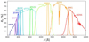 |
Fig. 1 Total transmission curves of the Javalambre filter system. On the vertical axis is the efficiency; the horizontal axis shows the wavelength in Angstroms. The efficiency includes contributions from filter transmission, atmosphere transmission, CCD efficiency, and primary mirror reflectivity curves. This photometric filter system is composed of seven narrow-band filters (J0378, J0395, J0410, J0430, J0515, J0660, and J0861) and five broadband filters (u, g, r, i, and z) (source: S-PLUS, 2019). |
Features of Javalambre system filters (S-PLUS, 2019).
2.2 APOGEE-2 spectroscopy
The Apache Point Observatory Galactic Evolution Experiment (APOGEE-2, Majewski et al. (2017)) from Sloan Digital Sky Survey-IV (SDSS-IV) DR17 (Abdurro’uf et al. 2022), hereafter APOGEE DR17, is a large-scale stellar spectroscopic survey conducted in the infrared (specifically in the H band, in the range 1.5μm < λ < 1.7μm) that acquires high-resolution spectra of R ~ 22 500. The main data products are spectra for individual and combined visits, measurements of radial velocity, atmospheric parameters (among them, effective temperature, surface gravity and metallicity) and abundances of individual elements. The stellar parameters and chemical abundances were determined from the APOGEE Stellar Parameters and Chemical Abundance Pipeline (ASPCAP, García Pérez et al. 2016). APOGEE-2 data has been used in multiple works to study the Milky Way’s structure, substructures, and satellite galaxies (e.g. Myeong et al. 2022; Horta et al. 2023; Limberg et al. 2022; Perottoni et al. 2022).
We used the following stellar parameters: effective temperature, Teff, surface gravity, log g, and metallicity, [M/H], to determine the labels for the algorithms. We limited the temperature in our sample to 3500 ≲ Teff (K) ≲ 7000 to avoid systematic problems (Abdurro’uf et al. 2022), and a signal-to-noise ratio of >20.
It is important to mention that [M/H] refers to the total metallicity adjusted to the full spectrum, and therefore has contributions from various metals. At the same time, the amount, [Fe/H], is a direct measurement of the Fe lines. The differences between the two parameters can be minor (Holtzman et al. 2015). In this work, we decided to use the [M/H] metallicity parameters because it is more representative of the total metallicity of the star.
2.3 Training, validation, and testing catalogue
We made a cross-match between the S-PLUS DR3 photometric data and APOGEE spectroscopic information to build the TVT catalogue. The cross-match was performed using Astropy (Astropy Collaboration 2013, 2018), selecting a maximum separation of 3.0 arcseconds between the positions. Within the search radius for each star, we kept only the closest matches within the search area. Considering only the entries containing metallic-ity information and accurate photometry in all S-PLUS bands, 24 924 unique stars were obtained.
From this sample, the stars that had a signal-to-noise s2n_[Filter]_PSTOTAL > 20 in all the S-PLUS bands were selected to define the TVT catalogue. The stars with flags PhotoFlag_[Filter] ≠ 0 − which excludes objects with contamination by neighboring sources, saturated pixels, truncated objects, etc. − were also eliminated, leaving a catalogue with 6433 stars, with −0.01 ≲ log g ≲ 5.19, − 2.45 ≲ [M/H] ≲ 0.50 and 3580 ≲ Teff (K) ≲ 6890.
Figure 2 shows the distribution of the TVT catalogue in the (log g, Teff) plane, including metallicity information in a colour bar. The typical 1σ uncertainties of these parameters are σteff ~ 36 K, σlogg ~ 0.063, and σ[M/H] ~ 0.075 dex, uncertainties much lower than those expected to be obtained using a photometric method, even based on NNs. This sample has a limit magnitude of r (mag) < 14.
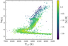 |
Fig. 2 Distribution of the 6433 stars resulting from the crossmatch between S-PLUS DR3 and APOGEE DR17 for the TVT catalogues in the Kiel diagram. The colour map represents spectroscopic metallicities. |
2.3.1 Defining labels for giants and dwarf stars
To implement a classification algorithm based on supervised learning, it is necessary to have labels that indicate to which class or category each object belongs. For this reason, we need to define some criteria to classify each star in the dataset as giant or dwarf. It is important to highlight that, among all the possible categories, in this work, we considered the stars to be either a giant or dwarf; for example, no additional categories were considered for sub-giant or asymptotic giant branch stars. A more detailed classification is not necessary for this work, since the importance of the classification lies in identifying the red giant stars among other stellar types. Red giant and dwarf stars can look very similar photometrically, and not knowing their distances, it may not be easy to distinguish which of them are dwarfs located in the solar neighbourhood and which are giants located at greater distances.
To establish the separation between the giant and dwarf stars in the TVT catalogue, we implemented a clustering algorithm by taking advantage of the parameter log g from APOGEE. In general, clustering algorithms allow the grouping of objects in a dataset so that the objects in the same cluster or group are more similar than those in other groups. In particular, we used the agglomerative hierarchical clustering algorithm AgglomerativeClustering from the module sklearn.cluster of scikit-learn (Pedregosa et al. 2011). For this task, the algorithm was implemented in such a way as to identify two groups in the plane (Teff, log g). Figure 3 shows the distribution of the two groups identified by the model: 1385 stars classified as giants (blue circles) and 4608 as dwarfs (red triangles).
Figure 4 shows the distribution of APOGEE DR17 spectroscopic metallicities of giant and dwarf stars classified by the clustering algorithm. Knowing this information is essential because the accuracy and robustness of a machine learning model depend on the data on which it is trained (Hettiarachchi et al. 2005). The range of the parameters of the training set – in this case, metallicities – is also essential to take into account, since the algorithms usually present significant errors when extrapolating (Wang et al. 2020).
We also tried to set the labels for the giant and dwarf stars using the Gaia DR3 data to generate a colour-magnitude diagram, MG versus G – R. We found that across Gaia 85.38% and 99.61% of the giant stars were recognised and dwarfs that were identified with APOGEE-2, respectively. The difference lies mainly in the area of the sub-giant stars, which the algorithm applied to the Gaia data recognised as dwarfs rather than giants. Since in this work we focus on red giant stars and since both classifications in this area coincided, we decided to use only the sample determined from APOGEE-2.
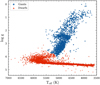 |
Fig. 3 Distribution of dwarf (red triangles) and giant (blue circles) stars determined by the hierarchical clustering algorithm in the (Teff, log g) plane. |
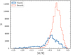 |
Fig. 4 Distribution of metallicities of giant (thick solid blue line) and dwarf (thin dashed red line) stars in the TVT set. Spectroscopic metallicities of giant stars have standard errors of σ ~ 0.02 dex and dwarfs of σ ~ 0.09 dex. |
2.3.2 Data augmentation
We applied data augmentation techniques to have a larger dataset to train, validate, and test the algorithms. This is a common practice in data science, since training models with more data usually improves their performance (Perez & Wang 2017; Wei et al. 2022). We performed the data augmentation by adding a random Δmag sampled randomly from a Gaussian distribution with a standard deviation equal to the reported photometric uncertainty to each S-PLUS band. We repeated this process 30 times for each star in the TVT catalogue. After performing the data augmentation process, the sample had 192 990 stars.
2.3.3 Catalogue homogenisation
As is shown in Figure 4, metal-rich stars are over-represented in the TVT catalogue (note that in the data augmentation procedure, the metallicity was not varied, so this distribution is equivalent to that obtained from the augmented dataset). Then, to ensure that the range of metallicities was equally represented, we cut the complete sample in −1.6 < [M/H] < 0.4 (since outside this range, the number of stars is much lower). The resultant sample was divided into bins of width equal to 0.05 dex, and 245 stars were randomly taken from each bin. This way, we obtained a homogeneous sample in metallicity with 9800 stars.
The sample of 9800 stars comprises the final TVT catalogue we use in our algorithms. For the training sample, 72% of the sample was used; for the validation sample, 8%; and for the test sample, the remaining 20%. The stars in each sample were selected randomly, and the proportions were chosen according to what is typical for this type of problem (Géron 2017).
3 Artificial neural networks
To classify the stars between dwarfs and giants and then determine their metallicities only from S-PLUS photometry, we built a series of ANNs using the dataset described in Section 2.3. The NNs were implemented in Python, specifically using version 2.7 of the TensorFlow library (Abadi et al. 2015).
The classification ANNs take colours determined from the photometric magnitudes of S-PLUS as input features, whereas they use the giant or dwarf categories determined by the clustering algorithm as labels (Section 2.3.1). The outputs delivered by the classification ANNs correspond to the probability of belonging to the giant or dwarf categories. On the other hand, the regression ANNs – the networks that determine the stellar metalicities as outputs – also take the photometric colours as input features and the spectroscopic metallicities of APOGEE DR17 as labels.
3.1 Input features
To find the combination of photometric colours that best performs both the classification and regression problems, we carried out an empirical procedure, testing all the possible combinations according to the following constraints:
We considered all colours determined from each narrowband filter and the broadband filter it overlaps, since these colours correspond to spectral indices for the spectral features. These colours are: (J0378 - u), (J0395 - g), (J0410 - g), (J0430 - g), (J0515 - g), (J0660 - r), and (J0861 - z).
We considered the colours determined from all possible combinations between broad-band filters, as these colours generally deliver temperature information or, in some cases, are sensitive to metallicity (especially in blue bands). These colours are: (u - g), (u - r), (u - i), (u - z), (g - r), (g - i), (g - z), (r - i), (r - z), and (i-z).
The colour combinations used to train the networks have between three and seven colours defined using one narrowband colour index and one or two colours defined only from wide-band colours.
Under these considerations, we obtained a total of 5445 colour combinations to use as input features in the designed networks (using one combination per training). The best ANN was chosen based on the classification or regression problem metrics.
3.2 Architecture and hypertuning
The architecture of the ANNs was determined through a hyperparameter tuning or hypertuning process carried out with Keras-Tuner (O’Malley et al. 2019), an easy-to-use Keras-integrated hyperparameter optimisation framework. The hypertuning process was performed ten times for a selected combination for each number of input colours (five combinations in the case of 3–7 narrow-band filter colours plus one broadband filter colour and five combinations in the analogous case with two broadband filters). The colours we used as inputs for hypertuning processes were chosen based on the highest mean signal-to-noise ratio in the filters that compose them.
The parameters adjusted were:
Number of hidden layers: between one and five;
Number of units of each hidden layer: multiples of 32 between 32 and 512;
Activation function for each hidden layer: relu, sigmoid or tanh;
Dropout layers: with fractions between 0.0 and 0.3;
Learning rate: 1e-1, 1e-2, 1e-3, or 1e-4.
We used an Adam optimiser (Kingma & Ba 2017), with a sparse categorical cross-entropy loss function for the classification and mean square error for the regression. The performance of the ANNs was measured using the accuracy metric for the classification (which calculates how often the predictions equal the labels) and the mean absolute error (MAE) for the regression. We performed the hypertuning using the Hyperband tuner class (Li et al. 2018). Although KerasTuner comes with many optimisation algorithms built in, we choose Hyberband because of its quicker execution in comparison with other state-of-the-art optimisers. The best model is obtained according to the accuracy metric for each hypertuning process.
The output layers for the classification ANN were set with two fixed units (since we were classifying stars between two categories) with a softmax activation function (Géron 2017). For the output layer of the regression ANN, we set a single fixed unit, since only one parameter would be predicted (metallicity).
We performed the training with two different batch sizes for both problems: 64 and 2048.
It is important to note that a pre-processing layer was added to normalise the input features of each ANN. Although, when working with structured data, the importance of the normalisation of the input characteristics is more evident in problems with different orders of magnitude, we carried out this step since it decreases the convergence time of the algorithms (Grus 2019).
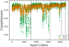 |
Fig. 5 Comparison of the completeness for giant (orange) and dwarf (green) stars for classification ANNs for different colour combinations as input features that include two broadband colours and trained with a batch size of 64. The horizontal axis indicates the unique ID associated with each colour combination (an integer between 0 and 4454). The four segmented vertical lines separate the combinations comprising different numbers of colours: IDs between 0 and 1574 indicate combinations made up of five colours, values between 1575 and 3149 indicate combinations of six colours, values between 3150 and 4094 indicate combinations of seven colours, between 4095 and 4409 for combinations of eight colours, and values between 4410 and 4454 for combinations of nine colours. Note that the segmented lines divide the figure according to the architecture of the ANN used for training and testing. |
4 Giant or dwarf classification
We trained the ANN 4,445 times, one for each combination of input colours described in Section 3.1, and using the architectures of the models determined with the hypertuning processes (see Section 3.2) with a batch size equal to 2048. The process was repeated for a batch size set to 64. Each of these ANNs was evaluated in the test set. Predictions were made, from which we obtained the completeness for giants and dwarfs (the fraction of stars correctly classified within a given actual class), the precision for giants and dwarfs (the fraction of stars correctly classified within a given predicted class), and the accuracy of the model (the fraction of stars correctly classified).
Next, we ranked the performance of the different ANNs according to the input colour combinations and all the metrics above, whereby a higher value implies a better performance.
Figure 5 shows the values obtained for completeness when evaluating the 4455 training runs executed for giants and dwarfs, including two broadband colours with a batch size of 64. The metrics with a batch size of 64 presented better results than the ones with a batch size of 2048. It should be noted that a graph like the one in Figure 5 by itself does not indicate which colours applied to the ANNs produce better or worse performance but show the general performance of specific architecture of the network tested. Information associated with each ANN should be examined separately to compare the performance of particular colour combinations.
Figure 5 also shows that dwarf stars have the highest completeness values, but generally, the networks manage to correctly identify more than 95% of the giants and dwarfs of the test set. This also happens with the networks trained with one broadband colour. Among the 990 ANNs with one broadband colour, 66 ANNs were able to correctly identify more than 98% of the giant and dwarf stars. Among the 4455 ANNs that included two broadband colours, 536 correctly identified more than 98% of the giant and dwarf stars. Specifically, the networks that identified a more significant number of dwarf and giant stars correctly used the input colours (J0378 - u), (J0395 - g), (J0410 - g), (J0515 - g), (J0660 - r), (g - z), and (r - i) (combination number 3324-2) and (J0378 - u), (J0395 - g), (J0410 - g), (J0515 - g), (J0660 - r), (J0861 - z), and (r - z) (combination number 948-1), respectively. Both ANNs, hereafter ANN-C3324-21 and ANN-C948-1, respectively, had an accuracy of 0.989. Both networks had the same architecture, consisting of five hidden layers, with 192, 96, 448, 224, and 96 units, respectively, with a relu activation function for the first two layers and tanh for the last. In addition, the architecture has four dropout layers with rates of 0.1 after the first, second, fourth, and fifth hidden layers. Next, we inspected both networks in deeper detail, and the ANN-C3324-2 was chosen to classify the stellar sources of S-PLUS, since the ANN-C948-1 learning curve presented a bit of overfitting in the validation set; in other words, the model began to ‘memorize’ the training data, which resulted in less precise outcomes on the validation set as a consequence.
Figure 6 presents the confusion matrix of the ANN-C3324-2, in which the predictions of the model using the test set can be visualised and compared to the actual classes (established by the clustering algorithm). It is important to note that these data have not been used in training, so theoretically they would show the actual performance of the ANN. The algorithm was able to correctly identify 1,939 stars that correspond to 98.92% of the test set. Specifically, it identified 98.83% of the giant stars and 99.03% of the dwarfs. Furthermore, 99.13% of the stars that the model identified as giants and 98.71% of the stars that the model identified as dwarfs coincided with the clustering algorithm labels.
Figure 7 shows the predictions of ANN-C3324-2 in the Kiel diagram, with the parameters Teff and log g of the APOGEE DR17 of the test set. It is observed that although the great majority of the stars identified as giants are located in the red giant branch, a few are scattered into the main-sequence turnoff. Something similar happens for the stars that the ANN classified as dwarfs, whereby some of them are found in the sub-giant branch. This is to be expected since, in this area, both populations have similar characteristics.
ANN-C3324-2 was trained with the combination of colours (J0378 - u), (J0395 - g), (J0410 - g), (J0515 - g), (J0660 - r), (g - z), and (r - i). The first five photometric indices correspond to the lines [OII], Ca H+K, Hγ, Mg triplet, and Hα, respectively. The magnesium triplet is a stellar surface gravity-sensitive feature (Majewski et al. 2000), so the best lattice would be expected to include the colour (F515 - g).
One way to validate the NN classification is to compare the stellar locus of giant stars in colour-colour diagrams with the predictions of synthetic stellar models. In Figure 8, we analyse the diagrams u − J0378 × g − z (top) and g − J0515 × u − z (bottom), in which giant stars present a clearly distinct locus in comparison to the overall distributions for the testing sample (left) and the full S-PLUS DR3 stellar catalogue (middle; see Section 6.1).
In the right panels of Figure 8, we plot a set of MIST isochrones (Dotter 2016), for the ages of 1, 3, 6, 9, and 12 Gyr, and metallicities of −2.0, −1.7, −1.5, −1.2, −41.0, −0.8, −0.5, and 0.0. Isochrones are colour-coded according to their theoretical log g, with blue lines representing the predicted colours of giant stars. For clarity, the giant stars in the testing sample are also shown in the right panels as black circles.
In general, we see that the giant stars classified by the NN indeed occupy the regions predicted by the synthetic models. We also see that, especially for giant stars, the S-PLUS narrow bands are particularly sensitive to metallicity, indicating that we can also measure this parameter for the classified giants.
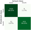 |
Fig. 6 Confusion matrix of the ANN-C3324-2 predictions for the test set, showing the number of actual and predicted stars in each category. |
 |
Fig. 7 Kiel diagram showing the predictions of ANN-C3324-2 for the test set. Stars classified by the ANN as dwarfs are shown as red triangles, and those classified as giants are shown as blue circles. |
5 Determination of stellar metallicities
Similarly to the classification procedure, we performed 5445 trainings, one for each colour combination described in Section 3.1, using the architectures derived from the hypertuning process introduced in Section 3.2 with batch sizes of 2048 and 64 for the entire set; and 5445 additional trainings for the giant stars only. We estimated the MAE for each ANN according to its performance in the evaluation of the test set and Equation (2):
![Mathematical equation: $\[M A E=\frac{1}{m} \sum_{i=1}^m\left|y_i-\hat{y}_i\right|\]$](/articles/aa/full_html/2024/11/aa51059-24/aa51059-24-eq2.png) (2)
(2)
where m is the total number of examples (in this case, stars), and yi and ![Mathematical equation: $\[\hat{y}_i\]$](/articles/aa/full_html/2024/11/aa51059-24/aa51059-24-eq3.png) are the predictions and actual values of the i-th example, respectively.
are the predictions and actual values of the i-th example, respectively.
Unlike the process carried out to determine the best network for the classification of stars, in this case we need to evaluate if developing separate models for giant stars – which is the objective of this work – is better for determining their metallicities than using a single network that determines the metallicities of all stars. To do this, we compared the performances of the two sets of NNs on all the colour combinations and selected the ones with the best performance using the MAE score. This metric is a measure of error, so a lower value represents a better performance.
Figure 9 shows the MAE of the two sets of ANNs trained with a batch size of 64 and using two broadband colours as input features. In this case, it was also observed that the ANNs trained with a batch size of 64 showed better results than the ones trained with a batch size of 2048. This is why the analysis focused on the first ANN (batch size of 64), with one and two broadband colours in the input features. Moreover, Figure 9 shows that the networks trained and validated with giant stars generally present more minor errors. This means that training ANNs separately for giant stars would give better results than using all the stars simultaneously. However, like in Figure 5 for the classification problem, this diagram does not provide greater detail. It is necessary to review some networks individually to determine which ones are best for tackling this regression problem.
From the analysis of the performance of the different trainings, we found that the networks trained only with giants had lower MAEs than those trained with all stars in 4308 cases. Additionally, 121 networks resulted in mean errors of less than 0.075 dex.
The network with the input colour combination 3292, hereafter ANN-R3292-22 - (J0378 - u), (J0395 - g), (J0410 - g), (J0515 - g), (J0660 - r), (u - g), and (r - z), the first five corresponding to the spectral characteristics [OII], Ca H+K, Hγ, Mg triplet and Hα, respectively – is the one with the best performance within the set of networks that used the complete TVT catalogue. In the case of networks trained, validated, and evaluated only with giant stars, the network that lead to the best performance was the one with the input colour combination 4290, hereafter ANN-R4290-23: (J0378 - u), (J0395 - g), (J0430 - g), (J0515 - g), (J0660 - r), (J0861 - z), (u - r), and (r - z), the first five corresponding to the spectral characteristics [OII], Ca H+K, G band, Mg triplet, Hα and Ca triplet, respectively. In both cases, Ca H+K and Mg triplet characteristics are present, which are sensitive to metallicity.
After selecting the best performing networks, we derived metallicities for the stars in the test set to assess the performance of the ANNs for the data that were not used in the training and validation steps. Figure 10 compares the predicted metallicities to the spectroscopic reference values from APOGEE. The predictions of metallicities of the most metal-poor stars tend to be slightly overestimated, and the most metal-rich ones underestimated. The standard deviation of the residuals – the difference between predicted and the reference (spectroscopic) values in the test set – is Δ[M/H] = 0.1 for ANN-R4290-2 and Δ[M/H] = 0.07 for ANN-R3292-2. As was expected, the network trained only with giant stars gives more accurate results.
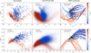 |
Fig. 8 Colour-colour diagrams u − J0378 × g − z (top) and g − J0515 × u − z (bottom), for the testing sample (left), whole S-PLUS DR3 (middle), and a set of theoretical MIST isochrones (right). The classified giant stars are shown in blue and the isochrones are colour-coded according to the predicted log g. |
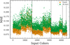 |
Fig. 9 Similar to Figure 5, but in this case the figure shows the comparison of the MAE in the predictions of metallicities. |
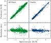 |
Fig. 10 Results of the inference of the ANN-R3292-2 for all stars (left, green) and the ANN-R4290-2 only for giants (right, blue) for the test set. The upper panels show the predictions vs the spectroscopic metallicities, and the lower panels show the residual for the metallicities. The grey area indicates a range of ±1 in standard deviation, which is 0.1 (dex) for all stars and 0.07 (dex) for giants only. The residuals were calculated as the difference between the predictions and the spectroscopic metallicities. |
Number of S-PLUS stars classified as giants and dwarfs by the ANN-C3324-2.
6 Derivation of metallicities for the whole S-PLUS stellar catalogue
In this section, we identify the giant stars and derive their metallicities using the ANNs designed and validated in the previous sections.
We applied the same quality cuts to the TVT catalogue to the complete S-PLUS DR3 catalogue; that is, a signal-to-noise ratio > 20 on each filter and flags = 0. Additionally, we selected data with CLASS_STAR > 0.75, consistent with the training set and with colours within limits set by the colours of the stars comprising the training set. These constraints guarantee that the stars of interest have similar photometric properties to the training catalogue, preventing the network from extrapolating.
With this dataset, we performed a cross-match with the Gaia EDR3 distance catalogue of Bailer-Jones et al. (2021). The search radius was set to 1.0 arcsecond, since, within this radius, unique matches were obtained for more than ~90% of the catalogue. The other ~10% had no match. The distances of 2 729 095 stars from S-PLUS DR3 were obtained.
6.1 Giant or dwarf classification with neural networks for the S-PLUS stellar catalogue
These 2 729 095 stars were classified as giants or dwarfs by the ANN-C3324-2 described in Section 4. The results of this process are shown in Table 2.
81% of the stars were classified as dwarfs, and the remaining 19% were classified as giants. This result is expected, since dwarf stars are more abundant, considering a magnitude limit of 20 in the r band given the applied signal-to-noise restrictions.
6.2 Determination of metallicities of giants
The photometric metallicities of the 523426 stars classified as giants were determined by the ANN-R3292-2, described in Section 5. Figure 11 shows the distribution of metallicity for giant stars. The values derived by the ANN lie between −1.9 < [M/H] < 0.5. This means that the network extrapolated some values; that is, by identifying stellar metallicities outside the set that was used to train it (−1.6, 0.4). A prominent peak is observed in the distribution around [M/H] ~−1.0. The catalogue with the photometric metallicities of the giants is available online4.
6.3 Metallicity distribution of giants in the Milky Way
The galactocentric (X,Y,Z) co-ordinates, indicated in Equations (3), were obtained from the Galactic co-ordinates, l and b, and the distances of Bailer-Jones et al. (2021). This information allows us to get the spatial distribution of metallicity of the S-PLUS stars in the Galaxy.
![Mathematical equation: $\[\begin{aligned}& X=R_{\odot}-d ~\cos (l) ~\cos (b), \\& Y=d ~\sin (l) ~\cos (b), \\& Z=d ~\sin (b)\end{aligned}\]$](/articles/aa/full_html/2024/11/aa51059-24/aa51059-24-eq4.png) (3)
(3)
where l and b are the galactic longitude and latitude, d the distances, and R⊙ = 8 kpc is the adopted distance from the Sun to the Galactic centre (Reid 1993; Camarillo et al. 2018). The centre of the (X,Y) plane is located in the Galactic centre. The X axis points to the Sun, the Z axis towards the North Galactic Pole, and the Y-axis is perpendicular to both, so the Sun’s rotation follows the positive direction of the Y axis. The (X,Y) plane is parallel to the plane of the Galaxy, and the Sun is at Z = 0. R is the distance to the centre of the Galaxy. The (X,Y,Z) co-ordinates make up the co-ordinate system ‘Galactocentric Cartesian co-ordinates’ and (R,Z) are the ‘Galactocentric cylindrical co-ordinates’.
Figures 12, 13 and 14 show the distribution of the giant stars of S-PLUS in the (X,Z), (Y,Z), and (X,Y) planes, respectively, along with their metallicities in the colour map. It is observed that stars become poorer in metals the farther from the Sun they are. Considering that the thin and thick discs of the Milky Way have a scale height of hZ ~ 300 pc and ~900 pc (Jurić et al. 2008), respectively, in Figures 12 and 13 metal-poor stars are found in the Galactic halo. However, it must be considered that despite Gaia’s precision, the uncertainties in the parallaxes for the most distant and faintest sources can become very large, which propagates into the distances of Bailer-Jones et al. (2021).
Figure 15 is complementary to Figures 12, 13 and 14, and shows the probability densities of the abundances in different ranges of R and Z. In the lower panels, |Z| < 2 kpc, the stars tend to be more metal-rich. This would indicate that, especially in the solar neighbourhood (panels |Z| < 2 kpc and 6 < R < 10 kpc), most of the observed stars belong to the Galactic disc. It can also be seen that only the panels of the solar neighbourhood show that the internal disc is more metal-rich than the outer one. It is also verified that the metallicity decreases when the distance to the Galactic plane increases. At |Z| > 6 kpc, the peak is around [M/H] ~−1.1.
Additionally, we computed the gradients in R and Z coordinates closer to the solar neighbourhood (solar neighbourhood assumed within one kpc). We obtained a vertical gradient of Δ[M/H]/Δ|Z| = −0.087 ± 0.002 dex kpc−1 (7 < R (kpc) < 9, |Z| (kpc) < 2) and a radial gradient of Δ[M/H]/ΔR = −0.193 ± 0.002 dex kpc−1 (6 < R (kpc) < 10, |Z| (kpc) < 1).
The radial metallicity gradient is compatible with the gradients of red giant stars of Hayden et al. (2014), Δ[Fe/H]/ΔR = −0.090 ± 0.002 dex kpc−1 (0 < R (kpc) < 15, 0.00 < |Z| (kpc) < 0.25) and Δ[Fe/H]/Δ|R| = −0.076 ± 0.003 dex kpc−1 (0 < R (kpc) < 15, 0.25 < |Z| (kpc) < 0.50). Otherwise, Huang et al. (2015) calculated radial gradients between Δ[Fe/H]/ΔR = −0.082 ± 0.003 dex kpc−1 and Δ[Fe/H]/ΔR = −0.020 ± 0.007 dex kpc−1 for |Z| ≤ 1.1 estimated for red clump stars.
Our vertical gradient is steeper than Boeche et al. (2014), Δ[Fe/H]/Δ|Z| = −0.112 ± 0.007 dex kpc−1 (at |Z| (kpc) < 2, and 7.5 < R (kpc) < 8.5, calculated with giants), and less steep than Hayden et al. (2014), Δ[Fe/H]/Δ|Z| = −0.305 ± 0.011 dex kpc−1 (at |Z| < 2), but is compatible with those of Huang et al. (2015), Δ[Fe/H]/Δ|Z| = −0.206 ± 0.006 dex kpc−1 (|Z| (kpc) < 1, 7 < R (kpc) ≤ 8) and Δ[Fe/H]/Δ|Z| = −0.116 ± 0.008 dex kpc−1 (|Z| (kpc) < 1, 8 < R (kpc) ≤ 9).
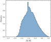 |
Fig. 11 Metallicity distribution of the giant stars of S-PLUS determined with the ANN-R3292-2. |
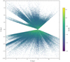 |
Fig. 12 Metallicity distribution of S-PLUS giant stars in the (X, Z) plane. The colour map indicates the metallicities. The Sun is located at (X, Z) = (8,0). |
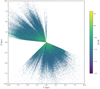 |
Fig. 13 Metallicity distribution of S-PLUS giant stars in the (Y,Z) plane. The colour map indicates the metallicities. The Sun is located at the point (Y,Z) = (0,0). |
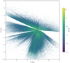 |
Fig. 14 Metallicity distribution of S-PLUS giant stars in the (X,Y) plane. The colour map indicates the metallicities. The Sun is located at(X,Y) = (0.8). |
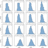 |
Fig. 15 Probability density of metallicities of giant stars of S-PLUS in different ranges of R and Z normalised to the number of giant stars in every panel. |
7 Conclusions
As a result of this work, we have shown that the application of machine learning methods to the problem of the derivation of stellar metallicities from a combination of broad and narrow-band photometry can achieve an accuracy comparable to medium-resolution spectroscopy but with the advantage of area coverage that current photometric surveys achieve.
The classification NN, which presented the best results in the classification of the test set, has five hidden layers and takes as input features the photometric colours (J0378 - u), (J0395 - g), (J0410 - g), (J0515 - g), (J0660 - r), (g - z), and (r - i), the first five corresponding to the spectral features from [OII], Ca H+K, Hδ, Mg triplet, and Hα, respectively. This network correctly identified 98.83 and 99.03% of the giant and dwarf stars in the test set, respectively. Among the stars that this model classified as giants, 99.13% were correctly classified, and among the stars that it classified as dwarfs, 98.71% were correctly classified.
It was found that the NNs for metallicity determinations developed specifically for giants produced more precise estimations than the networks trained with the complete sample of stars. The network that presented the lowest MAE over the test set, applied to the determination of photometric metallicities of giant stars, uses the colours (J0378 - u), (J0395 - g), (J0410 -g), (J0515 - g), (J0660 - r), (u - g), and (r - z) as input features, the first six corresponding to the spectral features from [OII], Ca H+K, Hδ, Mg triplet, and Hα, respectively. This network derived metallicities of stars in the test set with a standard deviation of σgiants ~ 0.07 dex with respect to the spectroscopic metallicities of APOGEE DR17.
Subsequently, both networks were applied to classify and determine the metallicities of a subsample of 2 729 095 stars from the S-PLUS DR3 catalogue. The algorithms identified 523 426 giant stars with metallicities between −1.9 < [M/H] < 0.5 with a peak at [M/H] ~−1.0. It is important to note that the performance of these methods on new data strongly depends on the training dataset. The method developed in this work could be improved by using more data for training. Still, our metallicity range for the training set is limited by the exclusive use of APOGEE-2 data. Yang et al., in prep., will provide a new calibration catalogue, extending the metallicity range down to [Fe/H] ~−4.0.
With the distances from Gaia EDR3, we constructed graphs of the spatial distribution of the metallicity of these stars in the Galaxy. Through this inspection, we found the most metal-rich stars in the Galactic disc region. However, when inspecting the distributions in different ranges in the R and Z co-ordinates, it was found that in the areas farthest from the Sun, the contribution of the giant stars of the halo begins to be more significant, represented as a peak of metal-poor stars at [M/H] ~−1.2. This contribution is even visible at the height of the Galactic plane but further from the Sun since, in the solar neighbourhood, the number of metal-rich stars is much larger.
Although our method is capable of performing a good (99.13% success) dwarf-giant separation, we note that our derived metallicities are not accurate below [Fe/H] < −1.5. This result is not unexpected given that the current training dataset, APOGEE-2 DR17, does not cover this low-metallicity regime with a sufficient number of stars (Limberg et al. 2022 for a recent discussion). In a future work, we plan to present novel strategies and calibrations for the estimation of precise [Fe/H] values for metal-poor stars.
Data availability
The catalogue is available at the CDS via anonymous ftp to cdsarc.cds.unistra.fr (130.79.128.5) or via https://cdsarc.cds.unistra.fr/viz-bin/cat/J/A+A/691/A144
Acknowledgements
This article is based on the research for the master’s thesis to obtain the title of MSc in Astronomy at the University of La Serena. F.M-J. acknowledges the partial financial support of DIDULS. The authors thank Stavros Akras, Alvaro Alvarez-Candal, Timothy Beers, Bruno Dias, Carlos Galarza, Guilherme Limberg, Lilianne Nakazono, Vinicius Placco and R. C. Thom de Souza for their detailed reading and suggestions that improved our manuscript. This work is based on data from S-PLUS. The S-PLUS project, including the T80-South robotic telescope and the S-PLUS scientific survey, was founded as a partnership between the Fundação de Amparo à Pesquisa do Estado de São Paulo (FAPESP), the Observatório Nacional (ON), the Federal University of Sergipe (UFS), and the Federal University of Santa Catarina (UFSC), with important financial and practical contributions from other collaborating institutes in Brazil, Chile (Universidad de La Serena), and Spain (Centro de Estudios de Física del Cosmos de Aragón, CEFCA). We further acknowledge financial support from the São Paulo Research Foundation (FAPESP), the Brazilian National Research Council (CNPq), the Coordination for the Improvement of Higher Education Personnel (CAPES), the Carlos Chagas Filho Rio de Janeiro State Research Foundation (FAPERJ), and the Brazilian Innovation Agency (FINEP). The authors who are members of the S-PLUS collaboration are grateful for the contributions from CTIO staff in helping in the construction, commissioning and maintenance of the T80-South telescope and camera. We are also indebted to Rene Laporte and INPE, as well as Keith Taylor, for their important contributions to the project. From CEFCA, we thank Antonio Marín-Franch for his invaluable contributions in the early phases of the project, David Cristóbal-Hornillos and his team for their help with the installation of the data reduction package JYPE version 0.9.9, César Íñiguez for providing 2D measurements of the filter transmissions, and all other staff members for their support with various aspects of the project. We also used data provided by SDSS. Funding for the Sloan Digital Sky Survey IV has been provided by the Alfred P. Sloan Foundation, the U.S. Department of Energy Office of Science, and the Participating Institutions. SDSS-IV acknowledges support and resources from the Center for High Performance Computing at the University of Utah. The SDSS website is https://www.sdss.org. SDSS-IV is managed by the Astrophysical Research Consortium for the Participating Institutions of the SDSS Collaboration including the Brazilian Participation Group, the Carnegie Institution for Science, Carnegie Mellon University, Center for Astrophysics | Harvard & Smithsonian, the Chilean Participation Group, the French Participation Group, Instituto de Astrofísica de Canarias, The Johns Hopkins University, Kavli Institute for the Physics and Mathematics of the Universe (IPMU) / University of Tokyo, the Korean Participation Group, Lawrence Berkeley National Laboratory, Leibniz Institut für Astrophysik Potsdam (AIP), Max-Planck-Institut für Astronomie (MPIA Heidelberg), Max-Planck-Institut für Astrophysik (MPA Garching), Max-Planck-Institut für Extraterrestrische Physik (MPE), National Astronomical Observatories of China, New Mexico State University, New York University, University of Notre Dame, Observatário Nacional / MCTI, The Ohio State University, Pennsylvania State University, Shanghai Astronomical Observatory, UnitedKingdom Participation Group, Universidad Nacional Autónoma de México, University of Arizona, University of Colorado Boulder, University of Oxford, University of Portsmouth, University of Utah, University of Virginia, University of Washington, University of Wisconsin, Vanderbilt University, and Yale University. This work has made use of data from the European Space Agency (ESA) mission Gaia (https://www.cosmos.esa.int/gaia), processed by the Gaia Data Processing and Analysis Consortium (DPAC, https://www.cosmos.esa.int/web/gaia/dpac/consortium). Funding for the DPAC has been provided by national institutions, in particular the institutions participating in the Gaia Multilateral Agreement.
References
- Abadi, M., Agarwal, A., Barham, P., et al. 2015, TensorFlow: Large-Scale Machine Learning on Heterogeneous Systems, software available from https://www.tensorflow.org [Google Scholar]
- Abdurro’uf, Accetta, K., Aerts, C., et al. 2022, ApJS, 259, 35 [NASA ADS] [CrossRef] [Google Scholar]
- Akras, S., Guzman-Ramirez, L., & Gonçalves, D. R. 2019a, MNRAS, 488, 3238 [NASA ADS] [CrossRef] [Google Scholar]
- Akras, S., Leal-Ferreira, M. L., Guzman-Ramirez, L., & Ramos-Larios, G. 2019b, MNRAS, 483, 5077 [NASA ADS] [CrossRef] [Google Scholar]
- Almeida-Fernandes, F. 2020, The S-PLUS Calibration Pipeline And schedule data releases, https://sites.usp.br/splus/wp-content/uploads/sites/846/2020/12/14_T_13_almeida-fernandes.pdf [Google Scholar]
- Almeida-Fernandes, F., SamPedro, L., Herpich, F. R., et al. 2022, MNRAS, 511, 4590 [NASA ADS] [CrossRef] [Google Scholar]
- Armandroff, T. E., & Da Costa, G. S. 1991, AJ, 101, 1329 [Google Scholar]
- Astropy Collaboration (Robitaille, T. P., et al.) 2013, A&A, 558, A33 [NASA ADS] [CrossRef] [EDP Sciences] [Google Scholar]
- Astropy Collaboration (Price-Whelan, A. M., et al.) 2018, AJ, 156, 123 [Google Scholar]
- Bailer-Jones, C. A. L., Rybizki, J., Fouesneau, M., Demleitner, M., & Andrae, R. 2021, AJ, 161, 147 [Google Scholar]
- Balas, V., Roy, S., Sharma, D., & Samui, P. 2019, Handbook of Deep Learning Applications, Smart Innovation, Systems and Technologies (Berlin: Springer International Publishing) [CrossRef] [Google Scholar]
- Baron, D. 2019, arXiv e-prints [arXiv:1904.07248] [Google Scholar]
- Bilicki, M., Hoekstra, H., Brown, M. J. I., et al. 2018, A&A, 616, A69 [NASA ADS] [CrossRef] [EDP Sciences] [Google Scholar]
- Boeche, C., Siebert, A., Piffl, T., et al. 2014, A&A, 568, A71 [NASA ADS] [CrossRef] [EDP Sciences] [Google Scholar]
- Camarillo, T., Mathur, V., Mitchell, T., & Ratra, B. 2018, PASP, 130, 024101 [NASA ADS] [CrossRef] [Google Scholar]
- Casagrande, L., Wolf, C., Mackey, A. D., et al. 2019, MNRAS, 482, 2770 [NASA ADS] [Google Scholar]
- Cenarro, A. J., Moles, M., Cristóbal-Hornillos, D., et al. 2019, A&A, 622, A176 [NASA ADS] [CrossRef] [EDP Sciences] [Google Scholar]
- Chambers, K. C., Magnier, E. A., Metcalfe, N., et al. 2016, arXiv e-prints [arXiv:1612.05560] [Google Scholar]
- Chiti, A., Frebel, A., Mardini, M. K., et al. 2021, ApJS, 254, 31 [NASA ADS] [CrossRef] [Google Scholar]
- Cole, A. A., Smecker-Hane, T. A., Tolstoy, E., Bosler, T. L., & Gallagher, J. S. 2004, MNRAS, 347, 367 [NASA ADS] [CrossRef] [Google Scholar]
- Dark Energy Survey Collaboration (Abbott, T., et al.) 2016, MNRAS, 460, 1270 [Google Scholar]
- Das, P., & Sanders, J. L. 2019, MNRAS, 484, 294 [NASA ADS] [CrossRef] [Google Scholar]
- Dias, B., & Parisi, M. C. 2020, A&A, 642, A197 [EDP Sciences] [Google Scholar]
- Dias, B., Barbuy, B., Saviane, I., et al. 2015, A&A, 573, A13 [NASA ADS] [CrossRef] [EDP Sciences] [Google Scholar]
- Dias, B., Barbuy, B., Saviane, I., et al. 2017, ASI Conf. Ser., 14, 17 [NASA ADS] [Google Scholar]
- Dotter, A. 2016, ApJS, 222, 8 [Google Scholar]
- Eggen, O. J., Lynden-Bell, D., & Sandage, A. R. 1962, ApJ, 136, 748 [NASA ADS] [CrossRef] [Google Scholar]
- Fluri, J., Kacprzak, T., Lucchi, A., et al. 2019, Phys. Rev. D, 100, 6 [CrossRef] [Google Scholar]
- Fukugita, M., Ichikawa, T., Gunn, J. E., et al. 1996, AJ, 111, 1748 [Google Scholar]
- Galarza, C. A., Daflon, S., Placco, V. M., et al. 2022, A&A, 657, A35 [NASA ADS] [CrossRef] [EDP Sciences] [Google Scholar]
- García Pérez, A. E., Allende Prieto, C., Holtzman, J. A., et al. 2016, AJ, 151, 144 [Google Scholar]
- Geisler, D. 1986, PASP, 98, 762 [NASA ADS] [CrossRef] [Google Scholar]
- Green, G. 2018, J. Open Source Softw., 3, 695 [NASA ADS] [CrossRef] [Google Scholar]
- Gruel, N., Moles, M., Varela, J., et al. 2012, SPIE Conf. Ser., 8448, 84481V [NASA ADS] [Google Scholar]
- Grunblatt, S. K., Zinn, J. C., Price-Whelan, A. M., et al. 2021, ApJ, 916, 88 [NASA ADS] [CrossRef] [Google Scholar]
- Grus, J. 2019, Data Science from Scratch: First Principles with Python (USA: O’Reilly Media) [Google Scholar]
- Gu, J., Du, C., Jia, Y., et al. 2015, MNRAS, 452, 3092 [NASA ADS] [CrossRef] [Google Scholar]
- Géron, A. 2017, Hands-on Machine Learning with Scikit-Learn and TensorFlow: Concepts, Tools, and Techniques to Build Intelligent Systems (USA: O’Reilly Media) [Google Scholar]
- Hayden, M. R., Holtzman, J. A., Bovy, J., et al. 2014, AJ, 147, 116 [NASA ADS] [CrossRef] [Google Scholar]
- Hettiarachchi, P., Hall, M. J., & Minns, A. W. 2005, J. Hydroinform., 7, 291 [CrossRef] [Google Scholar]
- Holtzman, J. A., Shetrone, M., Johnson, J. A., et al. 2015, AJ, 150, 148 [Google Scholar]
- Horta, D., Schiavon, R. P., Mackereth, J. T., et al. 2023, MNRAS, 520, 5671 [NASA ADS] [CrossRef] [Google Scholar]
- Huang, Y., Liu, X.-W., Zhang, H.-W., et al. 2015, Res. Astron. Astrophys., 15, 1240 [CrossRef] [Google Scholar]
- Huang, Y., Beers, T. C., Wolf, C., et al. 2022, ApJ, 925, 164 [NASA ADS] [CrossRef] [Google Scholar]
- IBM Cloud Education 2020, Deep Learning, https://www.ibm.com/cloud/learn/deep-learning [Google Scholar]
- Ivezić, Ž., Sesar, B., Jurić, M., et al. 2008, ApJ, 684, 287 [Google Scholar]
- James, D., Subramanian, S., Omkumar, A. O., et al. 2021, MNRAS, 508, 5854 [NASA ADS] [CrossRef] [Google Scholar]
- Jurić, M., Ivezić, Ž., Brooks, A., et al. 2008, ApJ, 673, 864 [Google Scholar]
- Kingma, D. P., & Ba, J. 2017, arXiv e-prints [arXiv:1412.6980] [Google Scholar]
- LeCun, Y., Bengio, Y., & Hinton, G. 2015, Nature, 521, 436 [Google Scholar]
- Li, L., Jamieson, K., DeSalvo, G., Rostamizadeh, A., & Talwalkar, A. 2018, J. Mach. Learn. Res. 18, 1 [Google Scholar]
- Limberg, G., Souza, S. O., Pérez-Villegas, A., et al. 2022, ApJ, 935, 109 [NASA ADS] [CrossRef] [Google Scholar]
- Lochner, M., McEwen, J. D., Peiris, H. V., Lahav, O., & Winter, M. K. 2016, ApJS, 225, 31 [NASA ADS] [CrossRef] [Google Scholar]
- López-Sanjuan, C., Yuan, H., Vázquez Ramió, H., et al. 2021, A&A, 654, A61 [NASA ADS] [CrossRef] [EDP Sciences] [Google Scholar]
- Mahabal, A., Sheth, K., Gieseke, F., et al. 2017, in IEEE Symposium Series on Computational Intelligence (SSCI) (USA: IEEE) [Google Scholar]
- Majewski, S. R. 2004, PASA, 21, 197 [NASA ADS] [CrossRef] [Google Scholar]
- Majewski, S. R., Ostheimer, J. C., Kunkel, W. E., & Patterson, R. J. 2000, AJ, 120, 2550 [NASA ADS] [CrossRef] [Google Scholar]
- Majewski, S. R., Schiavon, R. P., Frinchaboy, P. M., et al. 2017, AJ, 154, 94 [NASA ADS] [CrossRef] [Google Scholar]
- Marín-Franch, A., Chueca, S., Moles, M., et al. 2012, SPIE Conf. Ser., 8450, 84503S [Google Scholar]
- McMahon, R. G., Banerji, M., Gonzalez, E., et al. 2013, The Messenger, 154, 35 [NASA ADS] [Google Scholar]
- Mendes de Oliveira, C., Ribeiro, T., Schoenell, W., et al. 2019, MNRAS, 489, 241 [NASA ADS] [CrossRef] [Google Scholar]
- Miller, A. 2015, A Photometric Machine-Learning Method to Infer Stellar Metallicity (Berlin: Springer) [Google Scholar]
- Mitchell, T. 1997, Machine Learning, McGraw-Hill International Editions (New York: McGraw-Hill) [Google Scholar]
- Myeong, G. C., Belokurov, V., Aguado, D. S., et al. 2022, ApJ, 938, 21 [NASA ADS] [CrossRef] [Google Scholar]
- Öhman, Y. 1934, ApJ, 80, 171 [CrossRef] [Google Scholar]
- O’Malley, T., Bursztein, E., Long, J., et al. 2019, KerasTuner, https://github.com/keras-team/keras-tuner [Google Scholar]
- Pedregosa, F., Varoquaux, G., Gramfort, A., et al. 2011, J. Mach. Learn. Res., 12, 2825 [Google Scholar]
- Perez, L., & Wang, J. 2017, arXiv e-prints [arXiv:1712.04621] [Google Scholar]
- Perottoni, H. D., Limberg, G., Amarante, J. A. S., et al. 2022, ApJ, 936, L2 [NASA ADS] [CrossRef] [Google Scholar]
- Reid, M. J. 1993, ARA&A, 31, 345 [NASA ADS] [CrossRef] [Google Scholar]
- Sammut, C., & Webb, G. I., eds. 2010, Adaptive System (Boston, MA: Springer US), 35 [Google Scholar]
- Samuel, A. L. 2000, IBM J. Res. Develop., 44, 206 [CrossRef] [Google Scholar]
- Schlafly, E. F., & Finkbeiner, D. P. 2011, ApJ, 737, 103 [Google Scholar]
- Schlegel, D. J., Finkbeiner, D. P., & Davis, M. 1998, ApJ, 500, 525 [Google Scholar]
- Skrutskie, M. F., Cutri, R. M., Stiening, R., et al. 2006, AJ, 131, 1163 [NASA ADS] [CrossRef] [Google Scholar]
- Soumagnac, M. T., Abdalla, F. B., Lahav, O., et al. 2015, MNRAS, 450, 666 [NASA ADS] [CrossRef] [Google Scholar]
- S-PLUS. 2019, S-PLUS: Instrumentation, https://www.splus.iag.usp.br/instrumentation/ [Google Scholar]
- Thackeray, A. D. 1939, MNRAS, 99, 492 [CrossRef] [Google Scholar]
- Thomas, G. F., Annau, N., McConnachie, A., et al. 2019, ApJ, 886, 10 [NASA ADS] [CrossRef] [Google Scholar]
- Vivas, K. A., & Zinn, R. 2002, arXiv e-prints [arXiv:astro-ph/0212116] [Google Scholar]
- Walmsley, M., Smith, L., Lintott, C., et al. 2020, MNRAS, 491, 1554 [Google Scholar]
- Wang, B., Hu, S. J., Sun, L., & Freiheit, T. 2020, J. Manufactur. Syst., 56, 373 [CrossRef] [Google Scholar]
- Wang, C., Bai, Y., Yuan, H., et al. 2022, A&A, 664, A38 [NASA ADS] [CrossRef] [EDP Sciences] [Google Scholar]
- Warren, S. R., & Cole, A. A. 2009, MNRAS, 393, 272 [NASA ADS] [CrossRef] [Google Scholar]
- Wei, S., Chen, Z., Arumugasamy, S. K., & Chew, I. M. L. 2022, Environ. Sci. Ecotechnol., 11, 100172 [NASA ADS] [CrossRef] [Google Scholar]
- Whitten, D. D., Placco, V. M., Beers, T. C., et al. 2019, A&A, 622, A182 [NASA ADS] [CrossRef] [EDP Sciences] [Google Scholar]
- Whitten, D. D., Placco, V. M., Beers, T. C., et al. 2021, ApJ, 912, 147 [NASA ADS] [CrossRef] [Google Scholar]
- Wolf, C., Onken, C. A., Luvaul, L. C., et al. 2018, PASA, 35, e010 [Google Scholar]
- Yang, L., Yuan, H., Xiang, M., et al. 2022, A&A, 659, A181 [NASA ADS] [CrossRef] [EDP Sciences] [Google Scholar]
- Yip, K. H., Nikolaou, N., Coronica, P., et al. 2019, AAS/Division for Extreme Solar Systems Abstracts, 51, 305.04 [NASA ADS] [Google Scholar]
- York, D. G., Adelman, J., Anderson, John E., J., et al. 2000, AJ, 120, 1579 [NASA ADS] [CrossRef] [Google Scholar]
Code meaning: ANN - artificial neural network, C - Classification, 3324 - number of the combination, 2 - number of broadband colours used.
Code meaning: ANN - artificial neural network, R - regression, 3292 - correspond to the number of the colour combination, 2 - number of broadband colours used.
Code meaning: ANN - artificial neural network, R - regression, 4290 - correspond to the number of the colour combination, 2 - number of broadband colours used.
All Tables
All Figures
|
Fig. 1 Total transmission curves of the Javalambre filter system. On the vertical axis is the efficiency; the horizontal axis shows the wavelength in Angstroms. The efficiency includes contributions from filter transmission, atmosphere transmission, CCD efficiency, and primary mirror reflectivity curves. This photometric filter system is composed of seven narrow-band filters (J0378, J0395, J0410, J0430, J0515, J0660, and J0861) and five broadband filters (u, g, r, i, and z) (source: S-PLUS, 2019). |
| In the text | |
|
Fig. 2 Distribution of the 6433 stars resulting from the crossmatch between S-PLUS DR3 and APOGEE DR17 for the TVT catalogues in the Kiel diagram. The colour map represents spectroscopic metallicities. |
| In the text | |
|
Fig. 3 Distribution of dwarf (red triangles) and giant (blue circles) stars determined by the hierarchical clustering algorithm in the (Teff, log g) plane. |
| In the text | |
|
Fig. 4 Distribution of metallicities of giant (thick solid blue line) and dwarf (thin dashed red line) stars in the TVT set. Spectroscopic metallicities of giant stars have standard errors of σ ~ 0.02 dex and dwarfs of σ ~ 0.09 dex. |
| In the text | |
|
Fig. 5 Comparison of the completeness for giant (orange) and dwarf (green) stars for classification ANNs for different colour combinations as input features that include two broadband colours and trained with a batch size of 64. The horizontal axis indicates the unique ID associated with each colour combination (an integer between 0 and 4454). The four segmented vertical lines separate the combinations comprising different numbers of colours: IDs between 0 and 1574 indicate combinations made up of five colours, values between 1575 and 3149 indicate combinations of six colours, values between 3150 and 4094 indicate combinations of seven colours, between 4095 and 4409 for combinations of eight colours, and values between 4410 and 4454 for combinations of nine colours. Note that the segmented lines divide the figure according to the architecture of the ANN used for training and testing. |
| In the text | |
|
Fig. 6 Confusion matrix of the ANN-C3324-2 predictions for the test set, showing the number of actual and predicted stars in each category. |
| In the text | |
|
Fig. 7 Kiel diagram showing the predictions of ANN-C3324-2 for the test set. Stars classified by the ANN as dwarfs are shown as red triangles, and those classified as giants are shown as blue circles. |
| In the text | |
|
Fig. 8 Colour-colour diagrams u − J0378 × g − z (top) and g − J0515 × u − z (bottom), for the testing sample (left), whole S-PLUS DR3 (middle), and a set of theoretical MIST isochrones (right). The classified giant stars are shown in blue and the isochrones are colour-coded according to the predicted log g. |
| In the text | |
|
Fig. 9 Similar to Figure 5, but in this case the figure shows the comparison of the MAE in the predictions of metallicities. |
| In the text | |
|
Fig. 10 Results of the inference of the ANN-R3292-2 for all stars (left, green) and the ANN-R4290-2 only for giants (right, blue) for the test set. The upper panels show the predictions vs the spectroscopic metallicities, and the lower panels show the residual for the metallicities. The grey area indicates a range of ±1 in standard deviation, which is 0.1 (dex) for all stars and 0.07 (dex) for giants only. The residuals were calculated as the difference between the predictions and the spectroscopic metallicities. |
| In the text | |
|
Fig. 11 Metallicity distribution of the giant stars of S-PLUS determined with the ANN-R3292-2. |
| In the text | |
|
Fig. 12 Metallicity distribution of S-PLUS giant stars in the (X, Z) plane. The colour map indicates the metallicities. The Sun is located at (X, Z) = (8,0). |
| In the text | |
|
Fig. 13 Metallicity distribution of S-PLUS giant stars in the (Y,Z) plane. The colour map indicates the metallicities. The Sun is located at the point (Y,Z) = (0,0). |
| In the text | |
|
Fig. 14 Metallicity distribution of S-PLUS giant stars in the (X,Y) plane. The colour map indicates the metallicities. The Sun is located at(X,Y) = (0.8). |
| In the text | |
|
Fig. 15 Probability density of metallicities of giant stars of S-PLUS in different ranges of R and Z normalised to the number of giant stars in every panel. |
| In the text | |
Current usage metrics show cumulative count of Article Views (full-text article views including HTML views, PDF and ePub downloads, according to the available data) and Abstracts Views on Vision4Press platform.
Data correspond to usage on the plateform after 2015. The current usage metrics is available 48-96 hours after online publication and is updated daily on week days.
Initial download of the metrics may take a while.