| Issue |
A&A
Volume 663, July 2022
|
|
|---|---|---|
| Article Number | A106 | |
| Number of page(s) | 11 | |
| Section | Numerical methods and codes | |
| DOI | https://doi.org/10.1051/0004-6361/202243515 | |
| Published online | 21 July 2022 | |
New technique for determining a pulsar period: Waterfall principal component analysis
1
University of Padova, Department of Physics and Astronomy “Galileo Galilei”,
Via Marzolo, 8,
35131
Padova PD, Italy
e-mail: This email address is being protected from spambots. You need JavaScript enabled to view it.
2
Department of Electrical Engineering, Universidad de Chile,
Av. Tupper 2007,
Santiago
8370451, Chile
e-mail: This email address is being protected from spambots. You need JavaScript enabled to view it.
3
INAF Astronomical Observatory of Padova, Vicolo dell’Osservatorio, 5,
35122
Padova, Italy
4
University of Padova, Department of Information Engineering,
Via Gradenigo, 6/A,
35131
Padova PD, Italy
5
Trento Institute for Fundamental Physics and Applications,
Via Sommarive, 14
38123
Povo TN, Italy
Received:
10
March
2022
Accepted:
27
April
2022
Abstract
Aims. This paper describes a new technique for determining the optimal period of a pulsar and consequently its light curve.
Methods. The implemented technique makes use of the principal component analysis (PCA) applied to the so-called waterfall diagram, which is a bidimensional representation of the acquired data of the pulsar. In this context, we have developed the python package pywpf to easily retrieve the period with the presented method.
Results. We applied this technique to sets of data of the brightest pulsars in visible light that we obtained with the fast photon counter Iqueye. Our results are compared with those obtained by different and more classical analyses (e.g., epoch folding), showing that the periods so determined agree within the errors, and that the errors associated with the waterfall-PCA folding technique are slightly smaller than those obtained by the x2 epoch-folding technique. We also simulated extremely noisy situations, showing that by means of a new merit function associated with the waterfall-PCA folding, it is possible to become more confident about the determined period with respect to the x2 epoch-folding technique.
Key words: methods: data analysis / techniques: miscellaneous / pulsars: general
© T. Cassanelli et al. 2022
 Open Access article, published by EDP Sciences, under the terms of the Creative Commons Attribution License (https://creativecommons.org/licenses/by/4.0), which permits unrestricted use, distribution, and reproduction in any medium, provided the original work is properly cited.
This article is published in open access under the Subscribe-to-Open model. This email address is being protected from spambots. You need JavaScript enabled to view it. to support open access publication.
1 Introduction
High time resolution astrophysics (HTRA) investigates all types of celestial objects presenting rapid irradiance variability. Phenomena of interest include occultation measurements, oscillations in white dwarfs, flickering in cataclysmic variables, timing of pulsars, rapid variability in X-ray binaries, and accreting compact objects. Among these, pulsars are perhaps the most frequently studied HTRA objects because of their exotic nature and the possibility of investigating fundamental relativistic physical and astrophysical problems. A peculiar characteristic of these objects is their (quasi-) periodic signal, given by the combination of two factors: the beacon-like source that is due to an approximately conical light-emission beam of a very fast spinning neutron star, and the position of the Earth within the cone- scanned sky regions. With our instruments Aqueye/Aqueye+ (Barbieri et al. 2009a,b; Zampieri et al. 2015), applied to the Asiago Copernicus telescope (Italy), and Iqueye (Naletto et al. 2009), applied to the ESO New Technology Telescope (NTT; La Silla, Chile), we have investigated the visible light emitting pulsars that are accessible with medium size telescopes (Zampieri et al. 2011, 2014; Gradari et al. 2011; Germanà et al. 2012; Spolon et al. 2019). Only four of them can be seen with these telescopes: PSR B0531+21 (Crab pulsar), PSR B0540-69 in the Large Magellanic Cloud, PSR B0833-45 (Vela pulsar), and the most recent PSR J1023+0038 (Ambrosino et al. 2017; Zampieri et al. 2019); another pair of weaker optical pulsars (PSR B0656+14 and PSR B0630+17, also known as Geminga) are accessible only with larger telescopes (for the properties of optical pulsars, see, e.g., Mignani 2011).
One of the most important analyses to be performed on the pulsars is the determination of their (quasi) periods, P. In addition, because these objects lose energy by particle or light emission, their angular momentum varies in time, and the pulsation period slowly increases. Thus, from the analysis of the period variation in time, information can be obtained about the pulsar lifetime (∝P/P) and evolution. To retrieve the most accurate value of the pulsar period from the measured data, and consequently to obtain the best light curves, different techniques have been developed. These techniques depend on the data that can be obtained with the available instrumentation. For the best time resolution, the selected time bin has to be as small as possible: but reducing the time bin also implies that the collected signal per time bin becomes increasingly smaller, down to the limit of photon counting. Depending on the instrumentation performance, there are generally two types of dataset formats: if the time bin is relatively long with respect to the photon rate, practically all time bins have a nonzero value and the signal is essentially a continuous function of time; instead, if the time bin is too short, many bins have a zero signal and a few have a value of 1 or a few units, providing a Poisson distribution signal.
There is no clear evidence of a (quasi) periodicity (see for example Fig. 1) in these signals in general, and dedicated analysis tools are required to identify these features. We briefly review the most common techniques for determining the pulsar period, and then we describe how to obtain it by means of a novel technique that makes use of the principal component analysis (PCA). To do this, we investigated two different situations: one that we can define as low noise, for which a very simple algorithm can be used; and a second, the high noise, for which a suitable merit function had to be defined. The first situation applies to all the real cases we have investigated, which are the observations of the Crab pulsar taken in Asiago (Germanà et al. 2012), PSR B0540-69 (Gradari et al. 2011), and the Vela pulsar (Spolon et al. 2019) taken at the NTT in La Silla. The second situation has been reproduced artificially by adding noise to the Vela pulsar data. The obtained results not only agree with those obtained by means of other well-established techniques, but the use of PCA provides a higher level of versatility, which allows obtaining more confidence in the obtained results.
The structure of the paper is the following. Section 2 gives a brief description of the standard techniques typically used to estimate a pulsar period, and we also recall the description of the so-called waterfall diagram. In Sect. 3 a description of the PCA is given. Then, Sects. 4 and 5 explain the simplest way to apply the PCA to a waterfall diagram to determine the pulsar period, which corresponds to the low-noise case; the results obtained with this technique are also compared to those obtained by a more conventional technique. Finally, in Sect. 6 we describe the method (waterfall-PCA folding) used in the highest noise case, in which a dedicated approach had to be considered; moreover, a comparative analysis with the results obtained by a standard technique is provided. A summary of all the observations used for this analysis is reported in Table 1.
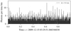 |
Fig. 1 Example of a light curve from the Crab pulsar (PSR B0531+21) acquired with Iqueye at NTT. Because the count rate is relatively low, with a time bin of ∆t = 0.1 ms, the periodic signal is not evident. |
Observations used in the waterfall-PCA folding analysis.
2 Common Techniques for Determining the Pulsar Period
To analyze pulsar data, the first convenient step is to identify the possible presence of a signal periodicity simply using a Fourier transform technique, for example, the fast Fourier transform (FFT). This is a very simple and straightforward method, but it has some intrinsic limitations: in some cases, periodic features are not so evident in an FFT, especially if the signal is rather noisy; the determination of the correct frequency is limited by the poor FFT frequency resolution, which depends on the number of input elements and on the ability of the software to deal with large arrays. In practice, because of these limitations, the FFT is used only for a preliminary identification of a possible periodic signal. When the periodicity is confirmed, more accurate analyses have to be performed to improve the frequency measurements.
A very well established technique for proceeding in the data analysis after having identified the periodicity, is to fold the signal, using the so-called epoch-folding technique (Leahy et al. 1983a,b; Leahy 1987; Gregory & Loredo 1992; Larsson 1996). In this case, a reasonable target period P is assumed either by the FFT analysis or by available information on the observed pulsar; then a trial period Pt relatively close to P is used to scan a suitable time region around P in search for the optimal period, P*. The search is realized by dividing Pt into N period time bins and coadding the pulsar timing data modulo Pt into these period time bins (the phase period is often used instead of the time period, with the phase period ranging between 0 and 1). By coadding (folding) the signal over a large number of periods, assuming the period constant over the time of folding, the statistics per period time bin is largely increased, and the pulse shape is generated. The more distant the trial period Pt from the actual period P*, the less accurate the light curve with respect to the correct light curve: to identify the best estimate of the actual period, and so to find the most accurate result, the standard procedure at this point is to vary the trial period by small amounts and to produce a set of light curves. By defining a suitable merit function and iterating the process searching for the highest merit function value, it is possible to increase the accuracy of the trial period and finally to obtain the optimum solution.
Thus, the problem of finding the best light curve is finally reduced to defining the optimal merit function. A fairly common algorithm used for this aim is calculating the χ2 value for the estimated light curve (Leahy et al. 1983a,b; Leahy 1987; Larsson 1996): it can be shown that the highest χ2 value provides the most accurate light curve. This approach is routinely adopted, and suitable algorithms can be found in dedicated software libraries (e.g., the timing analysis software for X-ray Astronomy xronos1 and stingray2). Other adopted techniques are the Z-test (Buccheri et al. 1983) and the H-test (de Jager et al. 1989; de Jager & Büsching 2010), which do not depend on the time binning.
Another accurate method that is not as frequently applicable, however, is the so-called waterfall diagram. The signal is folded to increase the statistics in this method as well, but the data analysis procedure is different. In this case, the total observation time is divided into M time intervals, usually with M ≥ 20, and folding is performed separately over each time interval with a common trial period Pt to obtain M light curves. Then, each light curve is stacked as a row in a matrix,

by associating a color scale with the intensity of the light-curve signal, this matrix can finally be represented as a color image.
This method allows detecting minute differences in the initial phase of the pulse even by simple visual inspection. An example is shown in Fig. 2, where the described method is applied with M = 200 to the analysis of the period of the Crab pulsar, OBS2. On the left, we show the image that is obtained when the trial folding period Pt differs from the actual period P* : it is clearly evident that the initial phase of the pulse changes because the folding period is incorrect, which produces tilted lines. Here we adopted a folding period Pt that largely differs from P* to exaggerate the visual effect, but it can be shown that this method is also very effective in measuring very small inclinations of the lines that correspond to very small deviations of the folding period from the actual one.
In practice, as in the previous case, the procedure to follow is to introduce small variations in the trial period Pt and to produce the corresponding waterfall diagrams; when the waterfall diagram shows straight vertical lines (see Fig. 2 right column), the best-fit period has been obtained. Notwithstanding its simplicity, the accuracy of this method is quite remarkable, and period values as accurate as those obtained by the epoch-folding technique can be obtained. An example of its accuracy is shown in Fig. 2, where a curvature of the vertical lines is visible, if not as clearly. This waterfall diagram has been obtained from a ~7200 s observation of the Crab pulsar by folding the data with a period that is correct at the middle of the observation and using M = 200. This residual curvature is due to the phase shift that occurred during the observing time as a consequence of the extremely low Crab pulsar regular spindown. This period variation can be measured with multiple observations, and at the time of observation (Zampieri et al. 2014), we obtained  this corresponds to a total change in the period of 3 ns from the beginning to the end of the observation, or equivalently, to a total phase variation of −0.0096. These numbers demonstrate the goodness of this method in highlighting these extremely small period or phase variations as well.
Unfortunately, this technique can only be applied with good results when the searched periodic signal is higher than the noise. When the noise is not negligible, the signal in the waterfall image has a very poor contrast, which makes detecting any periodicity very difficult. As an example, Fig. 3 shows the waterfall diagram for the PSR B0833-45 (OBS3; Table 1) using M = 20 and the nominal folding period: clearly, no straight vertical feature is evident, at least by eye.
The idea at the basis of this paper is to understand whether with a suitable software analysis, we can extract the hidden information of the actual pulsar period from waterfall images like the one shown in Fig. 3, where the human eye or simple techniques fail to detect any feature. We show that the PCA, which is widely used in many scientific applications, offers such a tool.
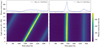 |
Fig. 2 Waterfall diagram of a two-hour Crab pulsar acquisition OBS2 (Table 1). The two columns have the same datasets, same number of divisions (M = 200), and time bin (∆t = 10 µs), but different trial periods Pt. Left column: Pt = 33.637 20 ms, and the right column has Pt = 33.637 26 ms, i.e., a difference of 60 ns. Top panels: average along the m-axis (number of divisions or number of light curves, |


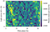 |
Fig. 3 Waterfall diagram for the PSR B0833-45 (Vela pulsar) observed for 180 min with Iqueye at the NTT (OBS3; Table 1). No vertical feature is evident, although the data have been folded in just M = 20 rows. The waterfall was generated with a Pt = 89.367 15 ms and a time bin of ∆t = 2.793 ms. |
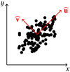 |
Fig. 4 For a bidimensional dataset with the distribution shown in this figure, the PCA allows defining the directions |


3 Principal Component Analysis
The PCA (Pearson 1901) is a mathematical tool that spans many fields of contemporary science: it is mainly used in image compression and more generally computer graphics, but also in statistics, mathematics, signal processing, meteorology, and so on. Depending on the field of application, this general technique is subject to small differences in implementation and so is often called in different ways: in computer graphics and in statistics, it is called PCA, in signal processing, it is better known as Karhunen-Loève transform (KLT; Karhunen 1947; Lévy & Loève 1948) and is used for very low signal-to-noise ratio denoising (while maintaining the basic characteristics of PCA, the algorithm and the method of application in this field are different from those of the PCA); other names by which this analysis technique is also known are independent component analysis (ICA; Hyvärinen et al. 2001), Hotelling transform (HT; Hotelling 1933, 1936), proper orthogonal decomposition (POD; see, e.g., Berkooz et al. 1993), and others.
The PCA is a relatively simple nonparametric method for extracting useful information from data that are otherwise difficult to interpret. Practically, the PCA is a way of identifying patterns in data and expressing the data in such a way as to highlight their similarities and differences: from a geometrical point of view, this corresponds to representing the data in a suitable reference frame such as to highlight their structure. For this, the algorithm uses an orthogonal transformation to convert a set of observations of possibly correlated variables into a set of values of uncorrelated variables called principal components (PCs). This transformation is defined in such a way that the first PC has as high a variance as possible (i.e., it accounts for as much of the variability in the data as possible), and each following component in turn has the highest possible variance under the constraint that it has to be orthogonal to (uncorrelated with) the preceding components.
As a simple example, we can think of a dataset with two variables represented in the xy reference frame (xy-basis) as the set of points shown in Fig. 4. The figure shows that the data have a principal direction of variation. This is identified with the u- axis. The second most important direction orthogonal to u is the v-axis. The PCA is a technique for identifying these two directions and to give them a priority on the basis of where the data have the largest dispersion. In practice, the PCA allows redefining the datasets in a new reference frame, on the uv-basis, which has its origin at the centroid of the data and is oriented in such a way as to obtain uncorrelated data, that is, their covariance with respect to the (u, v) coordinates is zero. The directions of these axes are the socalled PCs.
The algorithm for redefining the data with respect to the PCs is rather simple and consists of five steps. The first is to subtract the mean value of the data, which has to be done independently for the various variables: in the assumed two-dimensional data sample, the average value 〈x〉 (〈y〉) has to be subtracted from all the x (y) coordinates. Second, the covariance matrix C has to be calculated: in this example, C is a 2 × 2 matrix. The third step is calculating the eigenvectors eℓ and the corresponding eigenvalues λℓ of the covariance matrix. This process is equivalent to finding the reference frame in which the covariance matrix is diagonal, that is, where the variables are uncorrelated: in this reference frame, the covariances (i.e., the nondiagonal elements of the matrix) are all equal to zero, and only the variances (the diagonal elements) remain. The orientations of the axes of this reference frame are provided by the eigenvector set {e}, which constitute an orthonormal basis, and the corresponding eigenvalue set {λ} is equal to the variances along the directions of the corresponding eigenvectors eℓ. In the given example, the two eigenvectors provide the unitary direction vectors  and
and  shown in Fig. 4. The corresponding eigenvalues are equal to the variances of the data along these two directions, and the eigenvalue associated with the
  eigenvector is the highest.
In the fourth step, the eigenvectors are ordered by the corresponding eigenvalue from highest to lowest, to order the direction given by the eigenvectors in order of importance. If the ordered eigenvectors are used as columns of a matrix, a so- called feature vector F is obtained. In practice, this step allows prioritizing the PCs, with the most important ones retaining the largest amount of the data information. This is a very important step because it is possible to decide how much information of the original data to maintain by simply deciding how many PCs are used in the following step. If all the PCs are retained, all the information is preserved. Frequently, only the first ordered PCs have large variance, while the remaining ones provide a much smaller contribution: by discarding the less important PCs, the complexity of the system can be largely reduced (dimensional reduction) at the well-acceptable price of taking out only a minor amount of data information. With the final fifth step, the new dataset is obtained: the feature vector is used as a transformation matrix that takes the data points from the xy reference frame to the uv frame by means of the equation

where A(x, y) is a point in the xy reference frame, 〈A(x, y)〉 is the dataset centroid, and A(u, v) is the corresponding point in the uv reference frame.
Routines for applying PCA algorithms can be found in many libraries of commercial scientific standard packages3. For the data reduction that is specifically required for waterfall-PCA folding routines, the software pywpf4 has been developed, and it has been used throughout the following sections.
4 Application of the PCA to the Waterfall Diagrams of the Crab Pulsars
To verify the possibility of applying the PCA technique to the waterfall diagrams to determine the optimal folding period, some tests were made in the simplest case of the Crab pulsar (OBS2; see Table 1). The procedure we followed was first to produce different M × N waterfall diagrams  (with N = 336 number of columns, i.e., the number of time bins in the folding period, and M = 200 number of rows, i.e., the number of segments into which the whole acquisition has been divided), and then to vary the folding period Pℓ, where ℓ is the index associated with the trial period (and L is the total number of iterations). Figure 5 shows a graphical representation of the waterfalls while iterating over
  Then we applied the PCA to each of them, considering these waterfall images as M-dimensional datasets (i.e., a set of 336 200-dimensional hypervectors corresponding to the columns of the waterfall
  ). From this analysis, a set of M M-component eigenvectors eℓ,m with m = 1,…, M and of the corresponding eigenvalues λℓ,m were obtained per each waterfall
  with ℓ = 1,…, L. The eigenvalues obtained with the waterfall corresponding to the nominal period P* show that λ*;1, the one associated with the first PC eigenvalue, strongly dominated the others, providing a ratio

and all the components of the corresponding eigenvector e*,1 had substantially the same value  . This is an expected result: when the period is the best-fit period, all the rows of the waterfall are ideally identical, and so each hypervector is equal to the unitary hypervector multiplied by a constant, that is, the value of the signal intensity of the corresponding time bin. This means that in the 200-dimension space, the optimal M- dimensional dataset lies along the hyperdiagonal: in practice, all the points are aligned along this privileged direction. Along this direction, the dataset has the largest variance, which is the value provided by the eigenvalue, while in all the other perpendicular directions, the variance is almost null.
By analyzing the eigenvalues for the various waterfalls  , we also realized that the ratio Λℓ,1 has a peak in correspondence of the optimal folding period. These results suggested monitoring the behavior of the eigenvalue of the first PC eigenvector to estimate the best folding period. In Fig. 6 the first PC eigenvalue, λℓ,1 is shown. The folding period is changed multiple times, and when the peak is found, a smaller step can be defined, that is, ∆s = 1 ns for Fig. 6. In this case, the highest value of the first PC eigenvalue is easily found in correspondence of a pulsar period of PPCA = 33.637 261 ms: compared to the one provided by the Jodrell Bank monthly ephemerides (Lyne et al. 1993)5 at the same date of the Iqueye observations, a difference smaller than 0.2 ns can be found. This really remarkable result demonstrates the accuracy of this technique, at least for this simple case, which is definitely comparable to if not better than other standard and much more well-established techniques at long radio wavelengths.
From the obtained results in Fig. 6, we can now use the estimated period from the first PC eigenvalue and fold the dataset. In Fig. 7 we show the folded data when the maximum value from the first PC eigenvalue and the one from the Jodrell Bank monthly ephemerides are used (see Lorimer & Kramer 2012, Chapter 7). The Jodrell Bank period, PJB, was computed using PINT (Luo et al. 2021) referenced to SSB at the observed time stamps, then the average period over the whole recording was computed. The computed PJB takes the pulsar period into account: dispersion measure (DM),  and other parameters (at a fixed epoch) to predict the period at a certain time stamp t.
The application of the PCA to the waterfall diagrams allows an additional check of the goodness of the obtained results. Because ideally, at the optimal period P* the first PC eigenvector e*,1 should be parallel to the hyperdiagonal in the M-dimensional space, the optimal period can be obtained when the absolute value of the scalar product,
 (1)
(1)
of this eigenvector with the hyperdiagonal unitary vector  is maximum and ideally equal to 1. The behavior of the scalar product sℓ,1 in the previously examined case is shown in Fig. 8: this plot confirms the expected result: the largest scalar product corresponds to the nominal period. Furthermore, the value of the scalar product assumes values close to 1 only in a small range of the abscissa, with a discontinuity at about ±120 ns from the nominal period. Outside this range, the data are no longer well aligned, and the first PC eigenvector is far from being parallel to the hyperdiagonal. As we show in Sect. 6, this consideration can be used as a result quality check when the noise is much larger than in this case.
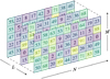 |
Fig. 5 Waterfall diagrams, W`, where each sheet has M × N dimension. M corresponds to the number of divisions (number of rows), N is the number given by the trial period Pℓ (i.e., Pt of the iteration ℓ) divided by a chosen time bin ∆t: N = round [Pℓ/∆t]. A data point has an amplitude given by the number of counts. L corresponds to the total number of trial periods Pℓ or number of iterations. For this particular case, L = 3, M = 5, and N = 9. The PCA is computed for every |

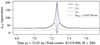 |
Fig. 6 First PC eigenvalue, λℓ,1 vs. folding period (∆s = 1 ns) for an acquisition of the Crab pulsar with Iqueye at the NTT, OBS2 (Table 1). For this case, M = 200 was chosen, and the best-fit period found was PPCA = 33.637 261 ms (with a search of L = 1000 iterations). Second and third eigenvalues,λℓ,2 and λℓ,3, are plotted as well. Their amplitude is significantly lower than λℓ,1, especially near PPCA. |
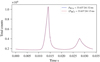 |
Fig. 7 Crab pulsar (PSR B0531+21) light curve obtained by folding the data with the period found using the maximum value of the first PC eigenvalue, PPCA (as shown in Fig. 6), and compared to the period from the Jodrell Bank monthly ephemerides, PJB. The Jodrell Bank period was computed using PINT at the observation time, and the period 〈PJB〉t was obtained by averaging over the whole transit (of duration t = 7200 s). The difference between the two methods is |ppca−〈pjb〉t|= 0·1766rn. |
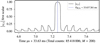 |
Fig. 8 Absolute value of the scalar product, |sℓ,1| (1), of the first PC eigenvector with the 200-dimension hyperdiagonal unitary vector as a function of the trial period in the case of the Crab pulsar. The scalar product (when a high signal-to-noise ratio is available) reaches magnitude i in a plateau region. Eigenvalue and scalar are plotted together in Fig. 15. The period PPCA was computed with the first PC eigenvalue, Fig. 6. |
5 Application of the PCA to the Waterfall Diagrams of Other Visible Pulsars
The same technique was applied to the more noisy cases of the other two optical pulsars we observed in 2009 with Iqueye at the NTT in La Silla (Chile): the PSR B0540-69 in the Large Magellanic Cloud (Gradari et al. 2011), and the PSR B0833-45 in the Vela supernova remnants (Spolon et al. 2019). To reduce the noise, it was necessary to take M ≤ 20 only in these cases.
As shown in the bottom panel of Fig. 9, which refers to an acquisition of about 58 min of the PSR B0540-69 (OBS1; see Table 1), the behavior of the first PC eigenvalue (λℓ,1) as a function of the trial period is rather noisy, and the peak is not as clearly defined as in the previous case. By means of a standard Gaussian fit, an improved estimated period can be found. The obtained peak period corresponds to PPCA = (50 663 540.00 ± 8.60) ns (with the reported error from the Gaussian peak position ±8.60ns). To cross-check the goodness of this result, we determined the best period on the same dataset also by means of the more well-established epoch-folding technique with χ2 optimum. The period obtained in this way is Px2 = (50 663 540.00 ± 4.34) ns, shown in the top panel of Fig. 9, where both periods agree within less than 10 ns (the time bin size ∆s).
Figure 9 also shows the Gaussian full width at half maximum (FHWM), which differs by 0.1 µs. Nevertheless, this simple estimated test shows that results from the epoch folding and the PCA are very similar, but epoch folding shows a clear noise reduction, that is, it is superior.
Finally, we also show here the results obtained in the case of the Vela pulsar (OBS3; Table 1). PSR B0540-69 is much less noisy than the Vela pulsar, which can be seen either in the epochfolding analysis or in the first PC eigenvalue of Figs. 9 and 10.
In Fig. 10 we have avoided to fit a Gaussian because the signal is too noisy to retrieve a good measurement. However, thereported periods by only taking the maxima reach very similar values. The difference between the two periods is ΔP = 120 ns.
We also monitored in these two cases the behavior of the scalar product sℓ,1 (1) between the first PC eigenvector and the unity vector parallel to the hyperdiagonal in the M-dimensional space (M = 20 in this case). The obtained results are shown in Fig. 11. These plots clearly show that the analysis of the scalar product sℓ,1 is not as sensitive as the analysis of the first PC eigenvalue, λℓ,1 for determining the optimal period: while Figs. 9 and 10 show a clear trend that allows accurately defining the highest value of the eigenvalue, in Fig. 11 it is much more difficult to determine the maximum in the scalar product. However, these plots allow us to unequivocally report that the optimal period is located in the region in which the absolute value of the scalar product is rather flat and reaches the highest values, higher than 0.8: this is a range of confidence that allows assessing that the inferred period is within a plateau of a flat region. Figures 9 and 10 also show that the same period we found from the first PC eigenvalue, PPCA, is within this high-amplitude region in Fig. 11.
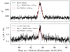 |
Fig. 9 First eigenvalue compared to epoch folding for PSR B0540-69. The top panel shows the χ2 optimization and the bottom panel the first PC eigenvalue for a waterfall |

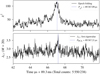 |
Fig. 10 First eigenvalue compared to epoch folding for PSR B0833- 45. The top panel shows the χ2 optimization and the bottom panel the first PC eigenvalue for a waterfall |

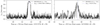 |
Fig. 11 Absolute value of the scalar product, |sℓ,1|, of the first PC eigenvector and the hyperdiagonal unit vector as a function of the trial period. Left: PSR B0540-69, same data as in Fig. 9. Right: PSR B0833-45, same data as in Fig. 10. In both cases, the optimum period lies within the plateau region, or where the maximum, ~1 is achieved. The dashed vertical line corresponds to PPCA, the optimum value found by the first PC eigenvalue (from Figs. 9 and 10). The same behavior is shown in the high signal-to-noise ratio case for PSR B0531+21 in Fig. 8. The total time and observation data are stated in Table 1. eported periods by only taking the maxima reach very similar values. The difference between the two periods is ∆P = 120ns. |
6 Performance in Case of a Noise-Limited Signal
To properly confirm the possible performance of the application of PCA to the waterfalls to determine the pulsar periods, we conducted a test to determine the limit for the detection of the optimal period when the noise was artificially increased. Then we compared the results with those obtained applying epoch folding and χ2 optimization under the same conditions.
To do this, we started with the same dataset as we used for the previous determination of the Vela pulsar period. This file collects the detection times of about 5.5 million photons, and the obtained optimal period is P* = 89 367.09 µs (top panel Fig. 10), as seen before. Producing the light curve with N = 32 phase bins (∆t ≃ 2.793 ms), the average counts per bin value are ~ 173 000, and the peak-to-valley (PtV) of the Vela pulsar pulse profile is just less than 1.6% of it (Spolon et al. 2019). Then we artificially increased the (white) noise by simply adding photon counts uniformly distributed in time. For example, adding another 5.5 million counts corresponds to twice the average with no change in the pulsar oscillation, and to bring the PtV to about 0.8%. We analyzed several cases for which we reduced the PtV value, and we stopped when we reached 23 million counts, which corresponds to a nominal PtV of less than 0.4%. Ideally, the noise addition does not alter the pulsar light curve, so that the expected determined optimal period should be noise independent. To produce a correct comparison between the two methods, all period searches were performed using the same initial trial period Pt = 89.367 ms, and the time events were binned at ∆t = 2.793 ms. The time period variation we used for the search was ∆s = 10 ns, which implies L = 1000 iterations in a time range of ±5µs around the nominal optimal period.
To quantify the goodness of the results when using the χ2 optimization, we adopted a confidence parameter  , defined as
 (2)
(2)
where  is the maximum of χ2, and
  and
and  are the average and the standard deviation ofχ2 outside the region of the peak. The quantity CP χ2 is substantially the signal-to-noise ratio for theχ2 function, but we prefer to call it differently because we consider the pulsar light curve as a signal on top of the background noise, and with this definition we avoid possible misunderstandings. A description of how to build the CP χ2 is shown in Fig. 12. We consider the period we found when CPχ2 ≳ 5 reliable. In the second column of Table 2, we report the CP χ2 value for some of the cases we analyzed. We can confirm the robustness of this technique because in all the cases, the procedure returned a period corresponding to the nominal one within the errors. However, as the top panel of Fig. 13, which corresponds to the χ2values for the most noisy case, clearly shows, the procedure determined the right value in this extreme case essentially by chance: the maximum of this function is a single isolated value above the average in the region of the correct period, but its significance is very poor (CPχ2 ≈ 2−3).
When we performed the analysis on these noisy datasets to search for the highest value of the first PC eigenvalue λℓ,1 we realized that even if this technique were a powerful tool for determining the periods for all the visible pulsars, its performance under these extreme conditions was not as good as the χ2 optimization: when we reached a total count of about 12–13 million, the peak of λℓ,1 was no longer discernible from the noise. However, we also realized the possibility of improving the algorithm performance by using the additional available piece of information, that is, the scalar product of the eigenvectors by the hyperdiagonal. The optimal period is associated with the maximum of the absolute value of the scalar product sℓ,m in (1), thus we can use it to define a new and very accurate merit function.
First, for each trial period Pℓ and the relative waterfall  we considered the highest absolute value sℓ,max of all the scalar products,

(when the situation becomes very noisy, it may happen that the first PC eigenvalue is no longer associated with the highest absolute value of the scalar product, but with the second or the third; because it is fundamental to find the eigenvector that is better coaligned with the hyperdiagonal in our analysis, we preferred to give priority to this parameter). Then, taken the λℓ,max eigenvalue, corresponding to the eigenvector eℓ,max which provides the maximum scalar product sℓ,max, we define
 (3)
(3)
as the waterfall-PCA folding merit function in correspondence to the trial period Pℓ. Figure 14 shows an example of this merit function with the Vela pulsar data, and Fig. 15 shows the same for the Crab pulsar, which is the case that is not limited by noise. Finally, we used the ξ-function in the same way as the χ2 in the previous analysis: we calculated all the ξℓ values as a function of the trial periods Pℓ, and obtained the optimal period when ξℓ is at its maximum value.
As an example, in Fig. 16 we compare the results of the optimal period Vela pulsar search using either χ2 or the ξ- function. The case ξℓ (M = 15) shows a clear and stronger central peak than the corresponding case shown in the bottom panel of Fig. 10, where only the first PC eigenvalue was used. The periods found using either the χ2 or the ξℓ (M = 15) functions have a difference on the order of nanoseconds, which is well within the errors.
During our analysis, we realized that using a different number M of divisions, slightly different results could be obtained (see, e.g., Fig. 17). Thus, we decided to provide a still more accurate merit function by averaging the obtained ξℓ for all the used values of M. For example, in this test, we varied M in the range M = 3, 4, …, 20 and obtained6
 (4)
(4)
To quantify the goodness of the results obtained by using Eq. (4), we defined a confidence parameter in this case as well,
 (5)
(5)
where 〈ξℓ〉m max is the maximum of 〈ξℓ〉m, and 〈ξℓ〉m avg and 〈ξℓ〉M rms are the average and the standard deviation of 〈ξℓ〉m out side the region of the peak. The corresponding expressions of Eq. (2) show that we can use these two parameters to compare the results of the two methods.
Column 3 in Table 2 provides the values for the confidence parameters CPξ determined in this case: by comparing these values with the corresponding  values, we can see that the waterfall-PCA folding technique provides some more confidence in the goodness of the results. Figures 17 and 18 show the change in the merit function with the number of division or when (white) noise is increased.
A better way to visualize how the average over M improves the waterfall-PCA folding function, 〈ξℓ〉M is shown in Fig. 19. This merit function waterfall (different from the light-curve waterfalls in Figs. 2 and 3) shows ξℓ = ξℓ(M), and the top panel takes the average over all M cases, Eq. (4). A clear noise reduction is visible because noise cancels out while the signal adds up. The computation of CPξ (third row Table 2) was made only over the average case with lower noise 〈ξℓ〉 M.
To further confirm the obtained results, this analysis was performed three times by adding (white) noise to the original signal with different random seeds. All three cases showed equivalent results, that is, equivalent numbers in Table 2.
Some considerations have to be made in relation to the analysis of the latter and more noisy case. This is a somewhat limiting situation for both techniques (see Fig. 13). For the epoch-folding χ2 technique, we verified not only that when the noise is increased, there is no longer a convergence on the optimal period, but also that changing the time bin in this case occasionally provides the determination of an incorrect period. For the waterfall-PCA folding technique, in 8 out of the 20 different checked M values, when the time bin was fixed, the algorithm returned the same incorrect peak as the χ2 peak. However, because of the possibility of having M – 3 datasets, we can be more confident about the goodness of the peak occurring with higher frequency. Moreover, because of this possible incorrect detection, we have to specify that the corresponding value of CP ξ reported in Table 2 was always calculated considering the peak measured at the nominal period, independently of the possible presence of other higher peaks. Figures 13 and 17 show that the incorrect detections are concentrated at the low M values, indicating that this technique is more accurate for high M values. The latter and noisiest case is a limiting situation for both techniques.
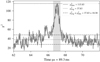 |
Fig. 12 Example calculation of the |


Values of the CPs for some of the cases we analyzed.
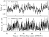 |
Fig. 13 Epoch-folding χ2 analysis and waterfall-PCA folding to search for the optimal period in the case of the maximum noise (23 million total counts; bottom row Table 2). Both methods have been set with the same time bin (∆t), start trial period, and step period increase (∆s). For comparison purposes, both datasets have been normalized by their maxima. |
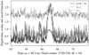 |
Fig. 14 Construction of the waterfall-PCA folding merit function / (3) for M = 10 for the Vela pulsar observation (no noise added). The plot shows three curves, the maximum scalar (1), the eigenvalue corresponding to the same sℓ,max, and the merit function ξℓ The merit function shows a clear and stronger signal-to-noise ratio than the scalar or eigenvalues alone. |
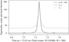 |
Fig. 15 Construction of the waterfall-PCA folding merit function ξℓ (3) for M = 200 for the Crab pulsar observation. The plot shows three curves, the maximum scalar (1), the eigenvalue corresponding to the same sℓt,max (high signal-to-noise ratio case corresponds to the first PC eigenvalue), and the merit function ξℓ The strength in signal-to-noise ratio for an ideal pulsar observation is clear. The scalar, very low with respect to the rest (with 1 the maximum amplitude) of the curves, is plotted in Fig. 8. Eigenvalues from the same dataset are shown in Fig. 6. |
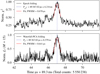 |
Fig. 16 Comparison epoch folding and waterfall-PCA folding for the original Vela pulsar data (total counts: 5 550 238 and ∆s = 10 ns). To facilitate comparison, both outputs (χ2 and ξℓ) were normalized by their maxima. The red line shows the best Gaussian fit with an error in the centered position of 6.216 ns and 8.379 ns for χ2 and ξℓ. Fig. 13 shows the same dataset when (white) noise is added. |
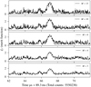 |
Fig. 17 Waterfall-PCA folding merit function, ξℓ, for waterfalls |

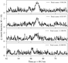 |
Fig. 18 Waterfall-PCA folding merit function, ξℓ, and its robustness while adding (white) noise to the data. The top row corresponds to the original Vela pulsar data (same as in Fig. 14). The noise increases from top to bottom. The number of divisions, M = 10, was kept fixed for all calculations. |
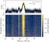 |
Fig. 19 Amplitude of each waterfall-PCA folding merit function,ξℓ (M3)(color map rows). Top panel: average of all M values, 3 ≤ M ≤ 20, and it is then plotted as a solid line. A scatter plot of the original data is overplotted (with the same amplitude color bar). There is a clear noise reduction in the 〈ξℓ〉 M computed with Eq. (4). The case corresponds to the nominal Vela pulsar of 5.5 million counts. The solid line has a CPξ = 8.9 (Table 2). Some discrete merit functions (rows in the color map) are plotted in Fig. 17. |
Future Considerations
Some additional points can be taken at the time to execute the PCA over these types of datasets. So far, we have assumed that no instrumental effect is added to our data, which is not true in principle. By observing an on and off pulse, a statistical information about the instrument itself can be extracted. This statistical information will be most sensitive when binning is applied to the data, which may change the data distribution. Using this additional statistical information from the observation, a weighted-PCA algorithm (Delchambre 2015) can be implemented to further consider the photon statistics, and to possibly improve the signal search. This is particularly important because the PCA method searches for the variance direction, but does not distinguish whether the variance comes from signal or from noise.
In addition, information from pulsars such as PSR B0531+21 might be used as timing calibrators in a nodding strategy. That is, PSR B0531+21 (calibrator) would be observed, then a nearby target source would be observed, and then again the calibrator. After this, we could examine the known drift in the rubidium clock and verify discrepancies with the GPS pulse-per-second timing correction (Naletto et al. 2009). A precise timing of the arrival wavefront will increase the performance of either waterfall-PCA or epoch folding. This is specifically suitable at the time when optical signals of pulsars are searched for that have not previously been seen at these wavelengths.
7 Conclusions
We have described a new technique, the waterfall-PCA folding, for obtaining the best period estimate of fast periodic objects like pulsars. A complete and easy-to-use python package has been developed for this purpose, pywpf.
This new technique is a rather powerful tool for performing this type of analysis. We applied it to data acquired with our instrument Iqueye (Table 1), which works in the visible light. The obtained results have been compared with those obtained by other more classical methods such as the χ2 epoch-folding technique. The performed analysis showed that the waterfall- PCA folding techniques works as expected and provides a small improvement over the classical method also in extremely noisy situations. The waterfall-PCA folding, in addition, allows verifying the goodness of the obtained results, providing a simple tool for determining whether the best-fit period is within the range of confidence.
Although a specific implementation is beyond the purpose of this work, this technique might in principle also be extended to other spectral ranges (e.g., infrared or X-rays) if significant photon-counting statistics are available. The required condition is that an adequate number of counts per period or bin can be collected in a rather limited interval of time (which is usually not the case for, e.g., the gamma-ray band), before the pulsar slowdown or timing irregularities start to significantly affect the accuracy of the period determination. In the latter case, the evolution of the pulsar period has to be incorporated in the analysis and a timing solution is needed. When it can be fruitfully applied, the waterfall-PCA folding also confirms the robustness of the results, providing a simple tool for exploring their confidence range.
Acknowledgements
This work is based on observations made with ESO Telescopes at the La Silla Observatory under programme IDs 082.D-0382 and 084.D-0328(A), and on observations collected at the Copernico Telescope (Asiago, Italy) of the INAF-Osservatorio Astronomico di Padova. We acknowledge the use of the Crab pulsar radio ephemerides available at the web site of the Jodrell Bank radio observatory (http://www.jb.man.ac.uk/~pulsar/crab.html; Lyne et al. 1993). Aqueye and Iqueye have been realized with the support of the University of Padova, the Italian Ministry of Research and University MIUR, the Italian Institute of Astrophysics INAF, and the Fondazione Cariparo Padova. L.Z. acknowledges financial support from the Italian Space Agency (ASI) and National Institute for Astrophysics (INAF) under agreements ASI-INAF I/037/12/0 and ASI-INAF n.2017-14-H.0 and from INAF “Sostegno allaricerca scientifica main streams dell’INAF” Presidential Decree 43/2018. We thank the developers of astropy (Astropy Collaboration 2013, 2018), numpy (Harris et al. 2020), scipy (Virtanen et al. 2020), matplotlib (Hunter 2007), and stingray (Huppenkothen et al. 2019). T.C. wishes to thank Paul Scholz and Jing Luo for their helpful discussions about epoch folding, radio pulsar folding, and X-ray observations.
References
- Ambrosino, F., Papitto, A., Stella, L., et al. 2017, Nat. Astron., 1 854 [NASA ADS] [CrossRef] [Google Scholar]
- Astropy Collaboration (Robitaille, T. P., et al.) 2013, A&A, 558, A33 [NASA ADS] [CrossRef] [EDP Sciences] [Google Scholar]
- Astropy Collaboration (Price-Whelan, A. M., et al.) 2018, AJ, 156, 123 [Google Scholar]
- Barbieri, C., Naletto, G., Occhipinti, T., et al. 2009a, J. Mod. Opt., 56 261 [NASA ADS] [CrossRef] [Google Scholar]
- Barbieri, C., Naletto, G., Verroi, E., et al. 2009b, Astrophys. Space Sci. Proc., 9 249 [NASA ADS] [CrossRef] [Google Scholar]
- Berkooz, G., Holmes, P., & Lumley, J. L. 1993, Ann. Rev. Fluid Mech., 25 539 [NASA ADS] [CrossRef] [Google Scholar]
- Buccheri, R., Bennett, K., Bignami, G. F., et al. 1983, A&A, 128 245 [NASA ADS] [Google Scholar]
- de Jager, O. C., & Büsching, I. 2010, A&A, 517, L9 [NASA ADS] [CrossRef] [EDP Sciences] [Google Scholar]
- de Jager, O. C., Raubenheimer, B. C., & Swanepoel, J. W. H. 1989, A&A, 221 180 [NASA ADS] [Google Scholar]
- Delchambre, L. 2015, MNRAS, 446 3545 [NASA ADS] [CrossRef] [Google Scholar]
- Edwards, R. T., Hobbs, G. B., & Manchester, R. N. 2006, MNRAS, 372 1549 [Google Scholar]
- Germanà, C., Zampieri, L., Barbieri, C., et al. 2012, A&A, 548, A47 [NASA ADS] [CrossRef] [EDP Sciences] [Google Scholar]
- Gradari, S., Barbieri, M., Barbieri, C., et al. 2011, MNRAS, 412 2689 [NASA ADS] [CrossRef] [Google Scholar]
- Gregory, P. C., & Loredo, T. J. 1992, ApJ, 398 146 [NASA ADS] [CrossRef] [Google Scholar]
- Harris, C. R., Millman, K. J., van der Walt, S. J., et al. 2020, Nature, 585 357 [NASA ADS] [CrossRef] [Google Scholar]
- Hobbs, G., Edwards, R., & Manchester, R. 2006, Chinese J. Astron. Astrophys. Suppl., 6 189 [NASA ADS] [CrossRef] [Google Scholar]
- Hotelling, H. 1933, J. Educational Psychol., 24 417 [CrossRef] [Google Scholar]
- Hotelling, H. 1936, Biometrika, 27 321 [CrossRef] [Google Scholar]
- Hunter, J. D. 2007, Comput. Sci. Eng., 9 90 [NASA ADS] [CrossRef] [Google Scholar]
- Huppenkothen, D., Bachetti, M., Stevens, A. L., et al. 2019, ApJ, 881 39 [Google Scholar]
- Hyvärinen, A., Karhunen, J., & Oja, E. 2001, Independent Component Analysis (New York: John Wiley & Sons, Inc.) [Google Scholar]
- Karhunen, K. 1947, Annales Academiae Scientiarum Fennicae, 37 1 [Google Scholar]
- Larsson, S. 1996, A&AS, 117 197 [NASA ADS] [CrossRef] [EDP Sciences] [Google Scholar]
- Leahy, D. A. 1987, A&A, 180 275 [NASA ADS] [Google Scholar]
- Leahy, D. A., Darbro, W., Elsner, R. F., et al. 1983a, ApJ, 266 160 [NASA ADS] [CrossRef] [Google Scholar]
- Leahy, D. A., Elsner, R. F., & Weisskopf, M. C. 1983b, ApJ, 272 256 [Google Scholar]
- Lévy, P., & Loève, M. 1948, Processus stochastiques et mouvements Browniens (Paris: Gauthier-Villars) [Google Scholar]
- Lorimer, D. R., & Kramer, M. 2012, Handbook of Pulsar Astronomy (Cambridge: Cambridge University Press) [Google Scholar]
- Luo, J., Ransom, S., Demorest, P., et al. 2021, ApJ, 911 45 [NASA ADS] [CrossRef] [Google Scholar]
- Lyne, A. G., Pritchard, R. S., & Graham Smith, F. 1993, MNRAS, 265 1003 [NASA ADS] [CrossRef] [Google Scholar]
- Mignani, R. P. 2011, Adv. Space Res., 47 1281 [NASA ADS] [CrossRef] [Google Scholar]
- Naletto, G., Barbieri, C., Occhipinti, T., et al. 2009, A&A, 508 531 [NASA ADS] [CrossRef] [EDP Sciences] [Google Scholar]
- Pearson, K.F.R.S. 1901, London, Edinburgh Dublin Philos. Mag. J. Sci., 2, 559 [CrossRef] [Google Scholar]
- Spolon, A., Zampieri, L., Burtovoi, A., et al. 2019, MNRAS, 482 175 [NASA ADS] [CrossRef] [Google Scholar]
- Virtanen, P., Gommers, R., Oliphant, T. E., et al. 2020, Nat. Methods, 17 261 [Google Scholar]
- Zampieri, L., Germanà, C., Barbieri, C., et al. 2011, Adv. Space Res., 47 365 [NASA ADS] [CrossRef] [Google Scholar]
- Zampieri, L., Cadež, A., Barbieri, C., et al. 2014, MNRAS, 439 2813 [NASA ADS] [CrossRef] [Google Scholar]
- Zampieri, L., Naletto, G., Barbieri, C., et al. 2015, SPIE Conf. Ser., 9504, 95040C [NASA ADS] [Google Scholar]
- Zampieri, L., Burtovoi, A., Fiori, M., et al. 2019, MNRAS, 485, L109 [NASA ADS] [CrossRef] [Google Scholar]
For example in python scikit-learn: https://scikit-learn.org
The pywpf package: https://github.com/tcassanelli/pywpf, developed by T. Cassanelli.
All Tables
All Figures
|
Fig. 1 Example of a light curve from the Crab pulsar (PSR B0531+21) acquired with Iqueye at NTT. Because the count rate is relatively low, with a time bin of ∆t = 0.1 ms, the periodic signal is not evident. |
| In the text | |
|
Fig. 2 Waterfall diagram of a two-hour Crab pulsar acquisition OBS2 (Table 1). The two columns have the same datasets, same number of divisions (M = 200), and time bin (∆t = 10 µs), but different trial periods Pt. Left column: Pt = 33.637 20 ms, and the right column has Pt = 33.637 26 ms, i.e., a difference of 60 ns. Top panels: average along the m-axis (number of divisions or number of light curves, |
| In the text | |
|
Fig. 3 Waterfall diagram for the PSR B0833-45 (Vela pulsar) observed for 180 min with Iqueye at the NTT (OBS3; Table 1). No vertical feature is evident, although the data have been folded in just M = 20 rows. The waterfall was generated with a Pt = 89.367 15 ms and a time bin of ∆t = 2.793 ms. |
| In the text | |
|
Fig. 4 For a bidimensional dataset with the distribution shown in this figure, the PCA allows defining the directions |
| In the text | |
|
Fig. 5 Waterfall diagrams, W`, where each sheet has M × N dimension. M corresponds to the number of divisions (number of rows), N is the number given by the trial period Pℓ (i.e., Pt of the iteration ℓ) divided by a chosen time bin ∆t: N = round [Pℓ/∆t]. A data point has an amplitude given by the number of counts. L corresponds to the total number of trial periods Pℓ or number of iterations. For this particular case, L = 3, M = 5, and N = 9. The PCA is computed for every |
| In the text | |
|
Fig. 6 First PC eigenvalue, λℓ,1 vs. folding period (∆s = 1 ns) for an acquisition of the Crab pulsar with Iqueye at the NTT, OBS2 (Table 1). For this case, M = 200 was chosen, and the best-fit period found was PPCA = 33.637 261 ms (with a search of L = 1000 iterations). Second and third eigenvalues,λℓ,2 and λℓ,3, are plotted as well. Their amplitude is significantly lower than λℓ,1, especially near PPCA. |
| In the text | |
|
Fig. 7 Crab pulsar (PSR B0531+21) light curve obtained by folding the data with the period found using the maximum value of the first PC eigenvalue, PPCA (as shown in Fig. 6), and compared to the period from the Jodrell Bank monthly ephemerides, PJB. The Jodrell Bank period was computed using PINT at the observation time, and the period 〈PJB〉t was obtained by averaging over the whole transit (of duration t = 7200 s). The difference between the two methods is |ppca−〈pjb〉t|= 0·1766rn. |
| In the text | |
|
Fig. 8 Absolute value of the scalar product, |sℓ,1| (1), of the first PC eigenvector with the 200-dimension hyperdiagonal unitary vector as a function of the trial period in the case of the Crab pulsar. The scalar product (when a high signal-to-noise ratio is available) reaches magnitude i in a plateau region. Eigenvalue and scalar are plotted together in Fig. 15. The period PPCA was computed with the first PC eigenvalue, Fig. 6. |
| In the text | |
|
Fig. 9 First eigenvalue compared to epoch folding for PSR B0540-69. The top panel shows the χ2 optimization and the bottom panel the first PC eigenvalue for a waterfall |
| In the text | |
|
Fig. 10 First eigenvalue compared to epoch folding for PSR B0833- 45. The top panel shows the χ2 optimization and the bottom panel the first PC eigenvalue for a waterfall |
| In the text | |
|
Fig. 11 Absolute value of the scalar product, |sℓ,1|, of the first PC eigenvector and the hyperdiagonal unit vector as a function of the trial period. Left: PSR B0540-69, same data as in Fig. 9. Right: PSR B0833-45, same data as in Fig. 10. In both cases, the optimum period lies within the plateau region, or where the maximum, ~1 is achieved. The dashed vertical line corresponds to PPCA, the optimum value found by the first PC eigenvalue (from Figs. 9 and 10). The same behavior is shown in the high signal-to-noise ratio case for PSR B0531+21 in Fig. 8. The total time and observation data are stated in Table 1. eported periods by only taking the maxima reach very similar values. The difference between the two periods is ∆P = 120ns. |
| In the text | |
|
Fig. 12 Example calculation of the |
| In the text | |
|
Fig. 13 Epoch-folding χ2 analysis and waterfall-PCA folding to search for the optimal period in the case of the maximum noise (23 million total counts; bottom row Table 2). Both methods have been set with the same time bin (∆t), start trial period, and step period increase (∆s). For comparison purposes, both datasets have been normalized by their maxima. |
| In the text | |
|
Fig. 14 Construction of the waterfall-PCA folding merit function / (3) for M = 10 for the Vela pulsar observation (no noise added). The plot shows three curves, the maximum scalar (1), the eigenvalue corresponding to the same sℓ,max, and the merit function ξℓ The merit function shows a clear and stronger signal-to-noise ratio than the scalar or eigenvalues alone. |
| In the text | |
|
Fig. 15 Construction of the waterfall-PCA folding merit function ξℓ (3) for M = 200 for the Crab pulsar observation. The plot shows three curves, the maximum scalar (1), the eigenvalue corresponding to the same sℓt,max (high signal-to-noise ratio case corresponds to the first PC eigenvalue), and the merit function ξℓ The strength in signal-to-noise ratio for an ideal pulsar observation is clear. The scalar, very low with respect to the rest (with 1 the maximum amplitude) of the curves, is plotted in Fig. 8. Eigenvalues from the same dataset are shown in Fig. 6. |
| In the text | |
|
Fig. 16 Comparison epoch folding and waterfall-PCA folding for the original Vela pulsar data (total counts: 5 550 238 and ∆s = 10 ns). To facilitate comparison, both outputs (χ2 and ξℓ) were normalized by their maxima. The red line shows the best Gaussian fit with an error in the centered position of 6.216 ns and 8.379 ns for χ2 and ξℓ. Fig. 13 shows the same dataset when (white) noise is added. |
| In the text | |
|
Fig. 17 Waterfall-PCA folding merit function, ξℓ, for waterfalls |
| In the text | |
|
Fig. 18 Waterfall-PCA folding merit function, ξℓ, and its robustness while adding (white) noise to the data. The top row corresponds to the original Vela pulsar data (same as in Fig. 14). The noise increases from top to bottom. The number of divisions, M = 10, was kept fixed for all calculations. |
| In the text | |
|
Fig. 19 Amplitude of each waterfall-PCA folding merit function,ξℓ (M3)(color map rows). Top panel: average of all M values, 3 ≤ M ≤ 20, and it is then plotted as a solid line. A scatter plot of the original data is overplotted (with the same amplitude color bar). There is a clear noise reduction in the 〈ξℓ〉 M computed with Eq. (4). The case corresponds to the nominal Vela pulsar of 5.5 million counts. The solid line has a CPξ = 8.9 (Table 2). Some discrete merit functions (rows in the color map) are plotted in Fig. 17. |
| In the text | |
Current usage metrics show cumulative count of Article Views (full-text article views including HTML views, PDF and ePub downloads, according to the available data) and Abstracts Views on Vision4Press platform.
Data correspond to usage on the plateform after 2015. The current usage metrics is available 48-96 hours after online publication and is updated daily on week days.
Initial download of the metrics may take a while.