| Issue |
A&A
Volume 663, July 2022
|
|
|---|---|---|
| Article Number | A113 | |
| Number of page(s) | 20 | |
| Section | Interstellar and circumstellar matter | |
| DOI | https://doi.org/10.1051/0004-6361/202141084 | |
| Published online | 22 July 2022 | |
Statistical properties and correlation length in star-forming molecular clouds
I. Formalism and application to observations
1
École normale supérieure de Lyon, CRAL, Université de Lyon,
UMR CNRS 5574,
69364
Lyon Cedex 07, France
e-mail: etienne.jaupart@ens-lyon.fr
2
School of Physics, University of Exeter,
Exeter,
EX4 4QL,
UK
e-mail: chabrier@ens-lyon.fr
Received:
14
April
2021
Accepted:
12
May
2022
Observations of molecular clouds (MCs) show that their properties exhibit large fluctuations. The proper characterization of the general statistical behavior of these fluctuations, from a limited sample of observations or simulations, is of prime importance to understand the process of star formation. In this article, we use the ergodic theory for any random field of fluctuations, as commonly used in statistical physics, to derive rigorous statistical results. We outline how to evaluate the autocovariance function (ACF) and the characteristic correlation length of these fluctuations. We then apply this statistical approach to astrophysical systems characterized by a field of density fluctuations, notably star-forming clouds. When it is difficult to determine the correlation length from the empirical ACF, we show alternative ways to estimate the correlation length. Notably, we give a way to determine the correlation length of density fluctuations from the estimation of the variance of the volume and column-density fields. We show that the statistics of the column-density field is hampered by biases introduced by integration effects along the line of sight and we explain how to reduce these biases. The statistics of the probability density function (PDF) ergodic estimator also yields the derivation of the proper statistical error bars. We provide a method that can be used by observers and numerical simulation specialists to determine the latter. We show that they (i) cannot be derived from simple Poisson statistics and (ii) become increasingly large for increasing density contrasts, severely hampering the accuracy of the high end part of the PDF because of a sample size that is too small. As templates of various stages of star formation in MCs, we then examine the case of the Polaris and Orion B clouds in detail. We calculate, from the observations, the ACF and the correlation length in these clouds and show that the latter is on the order of ~1% of the size of the cloud. This justifies the assumption of statistical homogeneity when studying the PDF of star-forming clouds. These calculations provide a rigorous framework for the analysis of the global properties of star-forming clouds from limited statistical observations of their density and surface properties.
Key words: methods: statistical / ISM: clouds / Oort Cloud / ISM: structure / ISM: kinematics and dynamics
© E. Jaupart and G. Chabrier 2022
 Open Access article, published by EDP Sciences, under the terms of the Creative Commons Attribution License (https://creativecommons.org/licenses/by/4.0), which permits unrestricted use, distribution, and reproduction in any medium, provided the original work is properly cited.
This article is published in open access under the Subscribe-to-Open model. Subscribe to A&A to support open access publication.
1 Introduction
Observations of molecular clouds (MCs) show that their main properties (velocity and column-density) exhibit large fluctuations. These fluctuations are at the heart of the star formation process (Padoan & Nordlund 2002; Mac Low & Klessen 2004; Hennebelle & Chabrier 2008; Hopkins 2012), implying that knowledge of their statistical characteristics is of prime importance. The accurate determination of the statistics of any quantity must rely on either a large enough number of samples or a large enough sample, so that a natural question arises: can we derive accurate statistical properties of MCs from observations, and if so how can we evaluate the level of accuracy? The relevance of a general statistical analysis of the global properties of MCs (e.g., mass, density PDF, temperature and velocity dispersion) deduced from observations and numerical simulations for studies of star formation processes must be assessed properly. For example, all of the theories that aim at determining the mass spectrum, that is the initial mass function (IMF) or the star formation rate (SFR) in a molecular cloud, rely on the assumption that a restricted number of observations or numerical simulations are representative of any MCs with similar properties (see e.g., Hennebelle & Chabrier 2008; Hopkins 2012; Vázquez-Semadeni et al. 2019 and reference therein). This key assumption must be tested.
Indeed, in studies of star formation based on observations or numerical simulations, one only has access to a small number of samples (and in reality only one most of the time). Therefore, in order to evaluate the statistics of the various stochastic fields of interest, one makes the basic assumption, sometimes called the “fair-sample hypothesis”, that the available sample is large enough for volumetric (or time) averages to be meaningful (see e.g., Peebles 1973 for a discussion in the context of cosmology). This assumption is only valid for stochastic fields that are statistically homogeneous and ergodic (Papoulis & Pillai 1965). Here, one should note that statistical homogeneity must not be confused with spatial homogeneity (we come back to this point below). The assumption of statistical homogeneity has been adopted by many authors, for example in studies of turbulent flows with or without self gravity (Chandrasekhar 1951a,b; Batchelor 1953; Pope 1985; Frisch 1995; Pan et al. 2018, 2019a,b; Jaupart & Chabrier 2020, 2021) and in cosmology for studies of the dynamics of structures in the Universe (Peebles 1973; Heinesen 2020). This assumption, however, provides no information on the magnitude of fluctuations around the average.
Quantifying (i) whether the “fair-sample hypothesis” is correct and, if so, (ii) what are the statistical error bars that derive from it, is an important issue when addressing PDF determinations in star-forming clouds. This is related to the completeness of the observations which we reformulate in this study in terms of statistical accuracy. In the context of the PDF of column-densities, (Alves et al. 2017), for instance, made an attempt to illustrate this problem by introducing the concept of open and closed density contours. These authors suggest that complete observations, that is considered as statistically significant and worth studying, correspond to closed contours. Although interesting, such an approach, however, can not be considered as a robust statistical determination of the bias and the statistical errors corresponding to incomplete observations of a cloud PDF. It is one of the very aims of this article to provide such a robust statistical analysis, using standard tools of random field theory and signal processing. Notably, one of the goals of the paper is to identify the statistical properties of the density field in a cloud inferred from column density data, and to derive procedures, based on the aforementioned tools, to accurately estimate these properties, whatever the PDF (lognormal or not). As such our approach does not make any assumption about the initial driving mechanism of the random motions responsible for the PDF of a cloud: turbulence or gravity.
The proper and standard way of addressing the previous issue relies on Ergodic theory. Ergodic Theory allows one to circumvent the problem of dealing with a single sample and to derive a robust measure of the accuracy of field statistics derived from the available data. In the present context, it also enables us to assess and quantify the relevance of a statistical approach on the evolution of star forming MCs. The key quantity is the correlation length, which is defined in terms of the integral of the auto-covariance function (see e.g., Papoulis & Pillai 1965). The fundamental result is that ergodic estimates are accurate if the dimensions of the sample, i.e. a whole cloud or part of it, are large enough compared to the correlation length. A proper determination of the correlation length in MCs is therefore of prime importance.
In pioneer works, (Scalo 1984); (Kleiner & Dickman 1985) studied the correlations of centroid velocities of the ρ-Oph and Taurus complex respectively and only found evidence of weak correlations at short scale on the order of their resolution. (Kleiner & Dickman 1984) studied the correlation of the column density field of the Taurus complex in search of a statistically significant length scale characterizing the separation of condensations within the complex but did not perform an evaluation of the correlation length, as defined above.
The objectives of this article are twofold. First, our main objective aims at examining the relevance and validity of a statistical approach based on ergodic theory to study the stochastic fields of star-forming MCs. Second, we seek to identify which statistical properties of the density field can be inferred from column density data and we derive procedures to obtain accurate estimates of these properties. The article is organized as follows. In Sect. 2, we outline the mathematical framework that yields the definition of the auto-covariance function (ACF) and correlation length of any statistical sample. In Sect. 3 we derive ways to determine the correlation length of any stochastic field without having to compute the ACF. In Sect. 4, we examine the case of astrophysical stochastic fields induced by compressible turbulent motions. In Sect. 5, we focus on the case of star-forming clouds and on the ways to infer the statistics of these fields from observations of column-densities. In Sect. 6, we apply our calculations to the typical star-forming cloud Polaris. We identify artifacts that are generated when one uses the statistical properties of the column-density field to infer those of the real density field; we show how to reduce these biases. In particular we derive a procedure to obtain proper error bars for the column density PDF. In Sect. 7, we examine the case of Orion B. Section 8 is devoted to the conclusion.
2 Methods: Mathematical Framework for a Statistical Approach
As mentioned in the introduction, a statistical approach of the properties of a cloud (or part of) is valid if this latter is large enough, compared to the correlation length of the quantity of interest, for the measured statistical quantities to be representative with high confidence of the genuine quantities. How to measure this confidence level and thus the relevance of a statistical approach is given by the ergodic theory, as commonly used in statistical physics or in the study of dynamical systems. Indeed, ergodicity implies by definition that different observations and realizations of a given statistical quantity yield results comparable enough for each of them to be representative of the average real quantity. It is described in the next section.
2.1 Ergodic Theory
We rederive here some ergodic theorems that lead to the definition of the correlation length. Let us consider a (scalar) stochastic field X(y), which depends on a D-dimensional position vector y (D = 1, 2 or 3). For a specific and fixed y, X(y) is a random variable of which we want to accurately determine the statistics.
2.1.1 Frequency Interpretation and Repeated Trials
The usual way to estimate the statistical average or expectation  of the random variable X(y) is to observe N samples X(y, ωi), 1 ≤ i ≤ N, of X(y) and to build the unbiased estimator
 (1)
(1)

where σ is the standard deviation (std). From Bienaymé-Tchebychev inequality (Papoulis & Pillai 1965), we know that, for any real number m > 0,
 (3)
(3)
where ℙ denotes the probability of a given event. We note that this inequality is valid for any random field, whether it is Gaussian or not. Although Tchebychev inequality gives a lower limit for the probability, it allows to give a confidence interval to measure the accuracy of the estimator given by Eq. (1). The larger the number of samples N, the smaller the std  and the more accurate the estimate in Eq. (1).
In case of statistical homogeneity for field X, the expectation  and std σ (X(y)) are no longer functions of the positions and one can drop the reference to y in Eqs. (2) and (3).
2.1.2 Ergodic Theorems, Autocovariance Function, Correlation Length
In the context of the study of MCs, one usually has only a single sample of X(y). As mentioned in the introduction, if one wants to be able to describe the stochastic fields at play, one assumes statistical homogeneity and build the unbiased estimator
 (4)
(4)
where ![$\Omega = {\left[ { - {L \over 2},{L \over 2}} \right]^D}$](/articles/aa/full_html/2022/07/aa41084-21/aa41084-21-eq8.png) is a control volume of linear size L and volume LD, which we want to be as large as possible 1. The ergodic estimator
is a control volume of linear size L and volume LD, which we want to be as large as possible 1. The ergodic estimator  has a variance
![${\mathop{\rm var}} \left( {{{\hat X}_L}} \right)\, = \,{1 \over {{{\left( L \right)}^D}}}\int_{{{\left[ { - L,L} \right]}^D}} {{C_X}\left( y \right)\,\coprod\limits_{k = 1}^D {\left( {1 - {{\left| {yk} \right|} \over L}} \right){\rm{d}}y,} } $](/articles/aa/full_html/2022/07/aa41084-21/aa41084-21-eq10.png) (5)
(5)
where  is the autocovariance function (ACF) of X at a lag y. The stochastic field X is said to be mean ergodic if the estimator
  converges toward
  as L → ∞ either in the mean square (MS) sense, meaning:
 (6)
(6)
or in probability meaning that, for every ϵ > 0,
 (7)
(7)
Bienaymé-Tchebychev inequality (Eq. (3)) not only shows that if X is MS mean ergodic  also converges in probability, but it also provides a confidence interval for the estimate
  . Slutsky’s theorem allows to write an equivalence for the ergodicity of X in a more convenient form: indeed, X is MS mean ergodic if and only if
![${1 \over {{{\left( L \right)}^D}}}\int_{{{\left[ { - L,L} \right]}^D}} {{C_X}\left( y \right){\rm{dy}}\mathrel{\mathop{\kern0pt\longrightarrow} \limits_{L \to \infty }} 0.} $](/articles/aa/full_html/2022/07/aa41084-21/aa41084-21-eq18.png) (8)
(8)
From there we obtain two sufficient (physical) conditions for X to be mean ergodic. Either:
 (9)
(9)

We assume both, and use the common definition of the correlation length lc(X) of the field X as a function of the ACF (Papoulis & Pillai 1965):
 (11)
(11)
This definition generalizes the usual definitions for 1D fields:
![${l_c}\left( X \right) = {1 \over {Cx\left( 0 \right)}}\int_{\left[ {0, + \infty } \right]} {{C_x}\left( y \right)} {\rm{d}}y\, = {1 \over {2{C_X}\left( 0 \right)}}\int_ {{c_X}\left( y \right)} {\rm{dy}}{\rm{.}}$](/articles/aa/full_html/2022/07/aa41084-21/aa41084-21-eq22.png) (12)
(12)
For lc(X) «L we then have from Eq. (5)
 (13)
(13)
where R = L/2. If we compare Eq. (13) with Eq. (2), we see that instead of having the number of samples, N, we now have the ratio (R/lc)D, where R (or L) is usually an observationally accessible quantity. We can thus interpret the ratio (R/lc)D as an effective number of “independent” samples. This result is of prime importance in the analysis of fluctuations within any stochastic field.
Furthermore, the correlation length is linked to the value of the power spectrum ƤX(k) of X at k = 0. Indeed
 (14)
(14)
2.1.3 Ergodic Hypothesis and Ergodic Theory
The results of ergodic theory derived above enable us to define under which conditions volumetric averages correspond to statistical averages and to provide a confidence interval for the estimate  of the expectation of X. However, these results rely on the knowledge of the statistical properties of X and more precisely of its ACF, which is in general not known. To apply this theory to the study of a real field, such as the density field for example, one must use ergodicity as an assumption. The above results can then be used to test the validity of this assumption and the accuracy of the estimates that are derived from it in a self-consistent way.
2.2 Estimates of the Autocovariance Function and Correlation Length
As shown in the previous section, the knowledge of the ACF of X (or of the value of the power spectrum of X at k = 0) is of crucial importance to measure the relevance of a statistical approach in studies of the properties of large (astrophysical) systems. In practice, however, the ACF of X must be evaluated from data.
2.2.1 Reliability of the Estimators of the Auto-Covariance and the Power Spectrum
In most cases, data are drawn from a finite size sample so that the ACF is not reliable at large lag (large scales). To simplify the notation, we now introduce the variable  and define the estimate, for a sample of size L,
 (15)
(15)
 (16)
(16)
This is an unbiased estimate of CX(y) but its variance is increasing as  and eventually becomes very large due to poor sampling. We thus introduce the biased estimate
 (17)
(17)
which is still a good estimate at small scales compared to L and has a reduced variance. We note however that it is an unbiased estimator of the quantity entering the integral in Eq. (5). Finally, it is also the Fourier Transform of the periodogram SL which is defined as:
![${S_L}\left( {\bf{K}} \right) = {1 \over {{L^D}}}{\left| {\int_{{{\left[ { - {L \over 2},{L \over 2}} \right]}^D}} {X\left( {\bf{y}} \right){e^{ik.y}}d{\bf{y}}} } \right|^{\rm{2}}}.$](/articles/aa/full_html/2022/07/aa41084-21/aa41084-21-eq31.png) (18)
(18)
It is the usual estimate of the power spectrum of X, ƤX. It is, however, a biased estimator of the power spectrum ƤX and is only unbiased asymptotically, in the limit L → ∞. Moreover, the variance of the estimator SL does not vanish as L → ∞ (Papoulis & Pillai 1965), which makes it quite unreliable.
We thus see that, because of the finite size of the sample, one cannot obtain a reliable estimate of the ACF (or of the power spectrum) for all lag values. Furthermore, in many cases, the mean value of X is not known and is replaced in Eq. (16) by its estimate  , which introduces further, but reasonable, bias (see Papoulis & Pillai 1965 for a more complete discussion).
2.2.2 Periodic Estimators
To get rid of the effect of finite sampling, one may perform simulations in periodic calculation boxes or may artificially add some periodicity to the available data to obtain the following estimate:
![${\hat C_{X{\rm{,per}}}}\left( {\bf{y}} \right) = {1 \over {{L^D}}}\int_{{{\left[ { - {L \over 2},{L \over 2}} \right]}^D}} {\left( {{X_{\hat \mu }}\left( {{\bf{y}} + {\bf{u}}} \right){X_{\hat \mu }}\left( {\bf{u}} \right)} \right)} {\rm{d}}u,$](/articles/aa/full_html/2022/07/aa41084-21/aa41084-21-eq33.png) (19)
(19)
where  and where one makes the identification
  . However, in such cases, the spatial average of the estimated ACF is necessarily 0. Indeed
![$\matrix{{\int_{{{\left[ { - {L \over 2},{L \over 2}} \right]}^D}} {{{{{\hat C}_{X,{\rm{per}}}}\left( {\bf{y}} \right)} \over {{L^D}}}d\,{\bf{y}}} } \hfill & = \hfill & {\int_{{{\left( {{{\left[ { - {L \over 2},{L \over 2}} \right]}^D}} \right)}^2}} {{{\left( {{X_{\hat \mu }}\left( {{\bf{y}} + {\bf{u}}} \right){X_{\hat \mu }}\left( {\bf{u}} \right)} \right)} \over {{L^{2D}}}}d{\bf{u}}\,{\rm{d}}{\bf{y}}} } \hfill \cr {} \hfill & = \hfill & {{{\left( {\int_{{{\left[ { - {L \over 2},{L \over 2}} \right]}^D}} {{{{X_{\hat \mu }}\left( {\bf{u}} \right)} \over {{L^D}}}{\rm{d}}{\bf{u}}} } \right)}^2} = 0,} \hfill \cr } $](/articles/aa/full_html/2022/07/aa41084-21/aa41084-21-eq36.png) (20)
(20)
due to the assumption that  is periodic.
Therein lies a significant problem: as the correlation length is defined as an integral over all possible lags, it is not easy to evaluate the reliability of estimates that are obtained in this manner.
Therefore, one traditionally produces an estimate for lc (or the integral scale li) in either of the next two ways. Either one searches for the e–1 value of the reduced ACF  to obtain an estimate of the correlation length (see e.g. Kleiner & Dickman 1984, 1985), assuming some exponential envelop for the ACF. Or, if the ACF decays fast enough at scales larger than lc(X), as is the case in turbulence (see previous section), the ACF is then generally extrapolated with a decaying exponential in regions where it becomes non monotonic (see e.g. Batchelor 1953; Reinke et al. 2016, 2018) so one can perform the integral and give a reliable estimate of lc(X) if lc(X) «L.
3 Fluctuations and Estimation of the Correlation Length
3.1 Expected Fluctuations in Repeated Trials
Be it for (numerical) experiments that can be repeated several times or for a statistically homogeneous and stationary field, volume averaged quantities fluctuate around their true expectations. In the former case, the volume averaged quantities fluctuate between the different samples while in the latter case they fluctuate in time. As we show in the following, these fluctuations depend on the ratio (lc/R). By studying these, we thus aim to obtain an accurate estimate of (lc/R), without having to calculate the ACF.
We consider here the case where one can reproduce several times the same experiment, as can be done for instance with numerical experiments or as can be approximated for clouds with similar conditions. We wish to determine the expected amplitudes of fluctuations of volume averaged quantities between samples.
To each experiment i of the N trials corresponds a value of the estimate  defined by Eq. (4). From Bienaymé-Tchebychev inequality, we know that
  lies around the true expectation
  within a distance such that, in probability,
 (21)
(21)
The average over the N trials (or sample average)
 (22)
(22)
is obviously a better estimate of  as
as
 (23)
(23)
We then expect the  to fluctuate around the sample average
  with variance
 (24)
(24)

If lc(X) is known, Eqs. (21), (24) and (25) allow one to give statistical error bars. Conversely, if lc(X) is not known, these equations give information on the product σ(X)(lc(X)/R)D/2 by performing the same statistical experiment several times and studying the dispersion of the  around
  .
.
Indeed, the half length l50%, of the segment centered on  within which 50% of the estimate
  falls, verifies2
 (26)
(26)
This gives a quick and easy qualitative determination of σ(X)(lc(X)/R)D/2. More quantitatively, the empirical variance of the sample of the N trials
 (27)
(27)
is an unbiased estimator of
 (28)
(28)
Computing the variance Var(N) thus yields an easy and rigorous method to determine (lc(X)/R)D and the correct error bars for statistical experiments.
3.2 Expected Temporal Fluctuations for a Statistically Homogeneous and Stationary Field
We consider here the case of a statistically homogeneous and stationary field (i.e., whose statistical properties are invariant under space and time translations). This can for example describe a steady turbulent flow (e.g. as simulated in a periodic box) without gravity.
As before, to each time t corresponds a value of the estimate  defined by Eq. (4) which lies around the true expectation
  within a distance such that, in probability,
 (29)
(29)
The time average over a large timescale T
 (30)
(30)
where t0 is a time at which the steady state is reached, is a better estimate of  as it has a variance
 (31)
(31)
where τc(XL) « T is the correlation time. Then, the signal  will fluctuate around
  with an empirical (temporal) variance
 (32)
(32)
which, providing that τc(XL) « T, is an accurate estimate of
 (33)
(33)
Hence, computing the variance VarT yields an easy and robust estimate of (lc(X)/R)D and the correct error bars for a statistically stationary field.
3.3 Fluctuations of Integrated Fields Overa Column
The previous cases work for experiments that can be repeated or for statistically stationary fields. However, in some situations, the two conditions cannot be fulfilled either because it is impossible to reproduce the experiment a large number of times or because the fields are not stationary (for instance in the presence of gravity).
In that case an estimate of ratio (lc/R) can be obtained if one has access to the integral of field X over a column of fixed length L = 2R:
![$\sum\nolimits_x {\left( r \right)} = \int_{\left[ {0,L} \right]} {X\left( {r,z,} \right)} {\rm{dz}},$](/articles/aa/full_html/2022/07/aa41084-21/aa41084-21-eq67.png) (34)
(34)
where r is a vector of D − 1 dimension (typically 2). The column must have a constant length to avoid creating spurious biases (see Sect. 5).
As ∑X/L corresponds to averaging X along one direction, we thus expect that its fluctuations will be reduced in comparison of those of X. The longer the length L of the column, the smaller the fluctuations of ∑X/L are expected to be. More quantitatively, the variance of ∑X/L is
 (35)
(35)
![$ = {1 \over {{L^2}}}\int_{{{\left[ {0,L} \right]}^2}} {{C_X}\left( {{\bf{0}},z - z'} \right)} {\rm{d}}z{\rm{d}}z'$](/articles/aa/full_html/2022/07/aa41084-21/aa41084-21-eq69.png) (36)
(36)
![$ = {1 \over L}\int_{\left[ { - L,L} \right]} {{C_\rho }\left( {{\bf{0}},u} \right)} \left( {1 - {{\left| u \right|} \over L}} \right){\rm{d}}u.$](/articles/aa/full_html/2022/07/aa41084-21/aa41084-21-eq70.png) (37)
(37)
A similar equation for the centroid velocities was given in (Scalo 1984). Now, if the ACF of X is isotropic at short lags and lc(X) « L, one can make the approximation
![${\mathop{\rm var}} \left( {{{\sum {_X} } \over L}} \right) \simeq {1 \over L}\int_{\left[ { - L.L} \right]} {C\rho \left( {\left| u \right|} \right){\rm{d}}u,} $](/articles/aa/full_html/2022/07/aa41084-21/aa41084-21-eq71.png) (38)
(38)
 (39)
(39)
where li(X) is the integral scale (Batchelor 1953) which, in most cases, verifies li(X) ≃ lc(X) (see Jaupart & Chabrier 2021). Thus a quick and easy estimate of ratio lc(X)/R is given by
 (40)
(40)
This method was applied to the density field (ρ = X) in (Jaupart & Chabrier 2021). The above estimate (Eq. (40)) was shown to produce the trends predicted analytically and thus to be a good approximation of the actual ratio lc(ρ)/R.
4 Application to Astrophysical Fields
The general results derived in Sect. 2 can be applied to many physical and astrophysical systems. They have been used extensively in cosmology but have somehow been overlooked in studies of star formation. Today, it is generally accepted that star formation is triggered by density fluctuations generated by compressible turbulence injected at a large scale in MCs (see e.g. McKee & Ostriker 2007 and reference therein). In this context, the density field ρ (or the logarithmic density field  ) is of prime interest and its cumulative distribution function (CMF) and probability density function (PDF) must be determined accurately.
Each of these statistical quantities is associated with a stochastic field X to which the results of Sect. 2 can be applied. For instance, the CMF Fρ(ρ0) at ρ0 is linked to the stochastic field hρ0(y) = Θ (ρ0 − ρ(y)) (where Θ is the Heavyside function), as
 (41)
(41)
while the PDF fρ(ρ0) is given by  where δρ0(y) = δ (ρ0 − ρ(y)) is Dirac’s distribution. Usually the PDF is rather deduced from histograms with some bin size ∆ρ such that
 (42)
(42)
In principle, knowledge of the ACF of all these fields is required to establish the accuracy of the estimations. Fortunately, it can be shown that sometimes, with a few simplifying assumptions, one can proceed with the ACF of ρ, only, in some situations. This is explained in detail in Appendix B.
4.1 Exact Results Regarding the Properties of the Auto-Covariance Function (ACF) ofρ
For a statistically homogeneous field, the ACF of ρ, the density field, can be expressed in term of the second order structure function:
 (43)
(43)
as  . A similar statement can be made for the logarithmic density field
  . This helps us to grasp some key features of the ACF. At very short scale (below the viscous scale), the density field is supposed to be differen-tiable and hence Cρ must possess second-derivatives at y = 0. Then, due to the parity of the ACF and because it is maximal at y = 0, its gradient must exist and be equal to 0 at y = 0.
Furthermore, (Jaupart & Chabrier 2021), generalizing the work of (Chandrasekhar 1951a), show that for a statistically homogeneous density field, the quantity
 (44)
(44)
is an invariant of the dynamics.
4.2 Phenomenology of (Compressible) Turbulence
The phenomenology of compressible turbulence (Kritsuk et al. 2007) can be derived, with some adjustments, from that of incompressible turbulence (Frisch 1995). Thus, we use the latter to derive some expected features of the density ACF in star-forming MCs that can be described by such phenomenology.
In isotropic turbulence, the second order structure function is observed to be a monotonic increasing function of separation distance, at least in the inertial range, and to converge rapidly toward 2Var (ρ) at scales that are larger than the integral scale li. This integral scale (not to be confused with the injection scale of turbulence, see Sect. 4.3) is defined in the same manner as the correlation length (Batchelor 1953)
 (45)
(45)
In many situations, lc ~ li, as shown in (Jaupart & Chabrier 2021). Thus, at small scales (short lags) and in the inertial range, the ACF must be a monotonically decreasing function. Above the inertial range, it is often assumed that the structure function and the ACF are still monotonic and the ACF is usually approximated by a decaying exponential, even though density fluctuations are likely to generate oscillations of the observed and estimated ACF as it tends to zero (Batchelor 1953; Reinke et al. 2016, 2018).
In compressible isothermal and stationary turbulence, the density field ρ is found to be approximately lognormal (Kritsuk et al. 2007; Federrath et al. 2010), implying that the logarithmic density field  is Gaussian with variance
  . In such Gaussian conditions, the ACFs of ρ and s are linked by the following equation:
 (46)
(46)
As a consequence, if Cρ (or Cs) is monotonically decaying toward 0, we deduce that:
 (47)
(47)
where we have used the following inequalities: eax − 1 ≤ x(ea − 1) for 0 ≤ x ≤ 1 and ax ≤ eax − 1 ∀x. For typical star forming conditions, σ(s)2 ≲ 4, implying that:
 (48)
(48)

This shows that under Gaussian conditions, for the two lengths lc(s) and lc(ρ), knowledge of one of them is sufficient to characterize the other one within an order of magnitude.
4.3 Large Injection Scale but small Correlation Length
Density and velocity fluctuations in MCs are thought to originate from turbulent motions driven at large scale (McKee & Ostriker 2007; Brunt et al. 2009), i.e. at scale comparable to the cloud scale L. This means that the energy of these turbulent motions is injected at an injection scale linj ~ L, below which the turbulent cascade eventually occurs.
The injection scale linj, however, is not the correlation length lc of either the velocity, kinetic energy or density fields. Otherwise, if linj = lc, every estimate produced from volumetric averages of the former fields would be inaccurate and far from the actual statistical values. This could result in large fluctuations of these averaged quantities either between different simulations (samples) or at different times for steady turbulent flows (see Sect. 3). What is instead observed in numerical simulations of compressible and steady turbulent flow is that volume averaged quantities of these fields display rather small fluctuations around their mean values. This is the case, for example, for the rms Mach number  , where υrms is the root of the volume average square velocity υ2 and cs the sound speed. To be more explicit,
![${{\cal M}^2} = {1 \over {{L^3}}}\int_{{{\left[ { - {L \over 2}.{L \over 2}} \right]}^3}} {{{{{\bf{v}}^2}\left( {\bf{y}} \right)} \over {c_s^2}}} {\rm{d}}{\bf{y}},$](/articles/aa/full_html/2022/07/aa41084-21/aa41084-21-eq90.png) (50)
(50)
so the result of Sect. 3 can be applied with  and
and  .
.
In (Federrath 2013), a series of numerical simulations of isothermal compressible turbulence driven to  with an injection scale linj = L/2 = R is presented. Once a statistical steady state is reached, the volume averaged Mach number
  (or
(or  which is a measure of the volume averaged specific kinetic energy) displays fluctuations that are rather small compared to their average values (their Fig. 1). Would we have lc(υ2) = linj = R, fluctuations of the signal
  would have yielded a temporal variance (Eq. (32)):
 (51)
(51)
from Eq. (33). Since the statistics of υ are close to being Gaussian (their Fig. A1), this would imply
 (52)
(52)
where  is the average of the signal
  over a time T. This would thus yield large fluctuations incompatible with their Fig. 1. The actual temporal variance VarT of signal
  in (Federrath 2013) rather yields a ratio
 (53)
(53)
which shows that lc(υ2) « linj = R.
Furthermore, (Jaupart & Chabrier 2021) used the estimate produced by Eq. (40) to compute the correlation length of the density field ρ. They found that within a factor of order unity,
 (54)
(54)
where λs is the sonic length which is found to be close to the average width of filamentary structures in isothermal turbulence (Federrath 2016).
The above results show that a large injection scale does not imply a large correlation length and that, on the contrary, correlation lengths in star-forming MCs are small compared with the injection scale (see above and Jaupart & Chabrier 2021).
4.4 Practical Assumptions Regarding the ACF
From the above results, we thus assume that the ACF decays rapidly at scales larger than the correlation length lc (lc ~ li, the integral scale) and then that the defining integral Eq. (11) can be calculated only up to a few lc. Moreover, we assume that the ACF can be bounded by a decaying exponential exp(−|y|/λ), where λ ~ lc above and in the inertial range to allow the computation of the correlation length (we note that such an exponential behavior is prohibited at very small scales due to the differentiability of ρ).
5 Star-Forming Clouds. Column Densities as Tracers of the Underlying Density Field
We now turn to observations of star-forming molecular clouds. Measurements provide values of the column-density ∑(x, y), which is the integral of density along the line of sight (l.o.s.(x, y)):
 (55)
(55)
where l(x, y) is the thickness of the cloud along the l.o.s. at (x, y) and  is the density fluctuation. Column densities are the only data that depend directly on the density field and one must determine how to retrieve reliable information from them.
5.1 Inhomogeneity and Anisotropy due to Integration over the Line of Sight
Star forming clouds are shaped by turbulent motions conferring statistical properties to their geometrical characteristics, and hence to the area projected in a plane perpendicular to the line of sight and to the thickness projected along the line of sight. This is responsible for difficulties in evaluating exactly the statistical average of ∑(x, y). However, provided that the cloud thickness is much larger than the correlation length, that is if l(x, y) » lc(ρ), we can reasonably assume that (see Eq. (55)):
 (56)
(56)
One must note here that we are dealing with the statistical average and not with the spatial average. This equation shows that ∑(x, y) may not be statistically homogeneous even if the density field ρ is, just because of integration effects. To illustrate this important point, let us imagine two idealized situations. In one of them, the cloud is a sphere of radius R. In the other one, the cloud is a “cube” of side L misaligned with the line of sight and seen from one of its edges such that the projected surface is of size  (see Fig. 1). For the sphere, the thickness along the line of sight is:
 (57)
(57)
whereas for the cubic cloud it is:
 (58)
(58)
Even though they are very simple, these two examples demonstrate that the column-density field may exhibit large-scale gradients and hence may not be statistically homogeneous, even if the density field is. Furthermore, as seen with the example of the cube, integration effects can also generate some anisotropy in the column-density field.
To reduce these effects, one can use a low pass filter to filter out large-scale gradients (Kleiner & Dickman 1984) and then treat the column density field as if it were homogeneous. Furthermore, most of the integration effects are expected to be produced by the first term of the r.h.s of Eq. (55). Thus they are expected to affect column densities that are around the (surface) average of the column density map 〈∑〉. In contrast, high column density (∑(x, y) > 〈∑〉, the regions of interest for star formation) are most likely to originate from the second term of the r.h.s of Eq. (55) and be produced by dense pockets along the line of sight. They are thus expected to be less affected by the integration effects and by the low pass filter. Studying the statistics of these high column density is thus expected to bear insights on the bias introduced by integration effects.
In Sect. 6, we will apply the above considerations to the observations of the Polaris cloud.
5.2 Column-Density Field in a Simulation Box
For a cubic simulation domain of size L, projecting the density field along one of the 3 principal directions of the cube leads to a statistically homogeneous column density field such that:
 (59)
(59)
The results of Sects. 2 and 3 can thus be applied with X = ∑ and the ACF of ∑ in this case is
![$\matrix{{{C_\sum }\left( {\bf{r}} \right)} \hfill & = \hfill & {\left( {\left( {\sum {\left( {{\bf{u + r}}} \right)} - \left( \rho \right)L} \right)\left( {\sum {\left( {\bf{u}} \right)} - \left( \rho \right)L} \right)} \right)} \hfill \cr {} \hfill & = \hfill & {\int_{{{\left[ {{{ - L} \mathord{\left/{\vphantom {{ - L} {2,}}} \right.\kern-\nulldelimiterspace} {2,}}{L \mathord{\left/{\vphantom {L 2}} \right.\kern-\nulldelimiterspace} 2}} \right]}^2}} {C\rho \left( {{\bf{r}},z - z'} \right){\rm{dzdz'}}} } \hfill \cr {} \hfill & = \hfill & {\int_{\left[ { - L,L} \right]} {C\rho \left( {{\bf{r,u}}} \right)} {\rm{d}}u\int_{ - L + \left| u \right|}^{L - \left| u \right|} {{{{\rm{d}}v} \over 2}.} } \hfill \cr {} \hfill & = \hfill & {L\int_{\left[ { - L,L} \right]} {{C_\rho }\left( {{\bf{r,u}}} \right)\left( {1 - {{\left| u \right|} \over L}} \right){\rm{d}}u.} } \hfill \cr } $](/articles/aa/full_html/2022/07/aa41084-21/aa41084-21-eq111.png) (60)
(60)
![${\rm{Var}}\left( \sum \right) = {C_\sum }\left( {\bf{0}} \right) = L\int_{\left[ { - L,L} \right]} {{C_\rho }\left( {{\bf{0}},u} \right)\left( {1 - {{\left| u \right|} \over L}} \right){\rm{d}}u} .$](/articles/aa/full_html/2022/07/aa41084-21/aa41084-21-eq112.png)
Then, if the density field is statistically isotropic at small scales (i.e. the ACF is isotropic at short lag) and lc(ρ) « L,
 (62)
(62)
Then Eq. (62) yields:
 (63)
(63)
which is a reformulation of Eq. (40). This is an important result because it gives a measure of lc(ρ)/R without having to compute the ACF. (Brunt et al. 2010); (Federrath et al. 2010) for example found a ratio Var  between 0.03 and 0.15.
(Vázquez-Semadeni & García 2001) were the first to study the impact of the lc(ρ)/R ratio on the statistics of column-density fields. Based on a crude interpretation of the central limit theorem (CLT), they proposed that, for lc(ρ)/R → 0, the column-density PDF should appear to be Gaussian instead of lognormal. This is not consistent with the apparent lognormality of the observed column-density PDFs, which led these authors to conclude that lc(ρ)/R cannot be vanishingly small and that it must be on the order of 10–1. However, the CLT only applies to independent variables and can hardly be valid for the sum ofcor-related variables, even if correlations decay. This casts doubt on the conclusions of (Vázquez-Semadeni & García 2001). More recently, (Szyszkowicz & Yanikomeroglu 2009) and (Beaulieu 2011) have shown that, for some special types of correlations, the sum of a large number N of lognormal variables tends to a lognormal distribution as N → ∞. We conclude that knowledge of the lc(ρ)/R value does not allow robust conclusions on the shape of the column-density PDF. However, as shown by Eq. (63), the variance Var  does become vanishingly small as lc(ρ)/R tends to zero. In that case, one can show with high probability that:
 (64)
(64)
Thus, in the limit of vanishing values of lc(ρ)/R, the distributions of  and its logarithm are both Gaussian if one of them is.
 |
Fig. 1 Projection of the two idealized situation. Left panel: case of a sphere. Right panel: case of a cuboid mis-aligned with the line of sight. |
5.3 Decay Length of Correlations
We now examine how the decay of correlations of ρ impacts the decay of correlations of ∑. For sake of simplicity, we again consider the case of a cubic box in order to avoid unncessary complications. For the 2D field ∑, the correlation length is given by:
![$\matrix{ {{l_c}{{\left( \sum \right)}^2} = {1 \over 4}{1 \over {{\rm{Var}}\left( \sum \right)}}\int\!\!\!\int {{C_{\sum \left( r \right)}}{\rm{d}}r,} } \cr { = {1 \over 4}{1 \over {{\rm{Var}}\left( \sum \right)}}\int\!\!\!\int L \int_{\left[ { - L,L} \right]} {{C_\rho }\left( {r,u} \right)\left( {1 - {{\left| u \right|} \over L}} \right){\rm{d}}u\,{\rm{d}}r} ,} \cr { \simeq 2{{L{\rm{Var}}\left( \rho \right)} \over {{\rm{Var}}\left( \sum \right)}}{l_c}{{\left( \rho \right)}^3}.} \cr } $](/articles/aa/full_html/2022/07/aa41084-21/aa41084-21-eq119.png) (65)
(65)
Using Eq. (62), this implies that:
 (66)
(66)
This shows that correlations of the column-density fields are decaying over a characteristic length close to lc(ρ), the correlation length of the underlying density field. In general, we can thus assume that lc(∑) ~ lc(ρ), so that information gathered from the column-density yields an estimate of the characteristic decay length of correlations of the underlying density field ρ.
6 Application to the Observations of the Polaris Cloud
As mentioned in Sect. 5, observations trace back the column-density (Kleiner & Dickman 1984; Schneider et al. 2015; Ossenkopf-Okada et al. 2016). These observations of the column-density PDFs in MCs show that regions where star formation has not occurred yet exhibit lognormal PDFs while regions with numerous prestellar cores develop power-law tails (PLTs) at high column densities (Kainulainen et al. 2009; Schneider et al. 2013). In addition to the integration effects yielding potentially the observed column-density to be anisotropic and inhomogeneous, observational data suffer further biases due to line of sight (l.o.s) contamination and noise (Schneider et al. 2015; Ossenkopf-Okada et al. 2016). L.o.s contamination causes two important biases. The observed power-law tail appears to be steeper than its corrected and uncontaminated counterpart while the observed variance in the lognormal part appears to be smaller than its corrected counterpart (Schneider et al. 2013). The overall effect of l.o.s contamination is to produce an underestimation of the total variance of the column-density.
6.1 Polaris
As a typical example of initial conditions of star formation in MCs, we focus on the Polaris flare, where line of sight contamination appears to be negligible (André et al. 2010; Miville-Deschênes et al. 2010; Schneider et al. 2013). Furthermore, most of the stellar cores in this cloud are still unbound (André et al. 2010), showing that star formation activity is very recent. Polaris is therefore a good candidate to probe the statistics of initial phases of star formation in MCs.
Data from Herschel Gould Belt survey extend across part of this cloud over approximately a 10 square degrees region with a linear size L ~ 10 parsecs (pc) (André et al. 2010). The cloud total mass and area above an extinction Av ≥ 1 are  and
and  , respectively. Dust temperatures are in a narrow Tdust = 13 + 1K interval, indicating fairly isothermal conditions with an average Mach-number
  (Schneider et al. 2013).
The Polaris logarithmic column-density field ŋ, where ŋ = ln(∑/ 〈∑〉), has a PDF with an extended Gaussian part and two emerging power-law tails, a first one with exponent αŋ,1 ≃ −4 followed by a shallower one with exponent αŋ,2 ≃ −2 (Fig. 2). (Jaupart & Chabrier 2020) have shown that the first steep PLT is due to gravity beginning to affect turbulence in parts of the cloud and hence records an early stage of (local) collapse. Furthermore the authors outlined a procedure to reconstruct the underlying logarithmic volume density PDF, noted s-PDF, where  , from data on the η-PDF. The underlying s-PDF displays a Gaussian part and two PLTs with exponents αS,1 = −2 and αS,2 = 3/2, respectively (see Fig. 2).
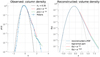 |
Fig. 2 Column and volume density PDF of the Polaris cloud. Left: Observed logarithmic column-density (ŋ = ln(∑/ 〈∑〉)-PDF (Schneider et al. 2013; Jaupart & Chabrier 2020). Right: Estimated and reconstructed underlying logarithmic density |

6.2 Filtering Large-Scale Gradients
As seen in Sect. 5, integration effects can produce large-scale gradients and break statistical homogeneity as well as isotropy in the column density field.
Filtered and unfiltered column-density maps of the Polaris flare are displayed in Figs. 3 and 4. The low pass filter does not alter qualitatively the intricate structures that exist, while the high-pass filter reveals a large-scale gradient likely due to integration effects. In order to partially reduce measurement artifacts, we use a low pass filter that screens out structures larger than L/2 in the column-density contrast (∑ − 〈∑〉), where L is the linear size of the observed region and we recall that 〈∑〉 is the (surface) average of the column density map. We can then treat the column-density field as if it was homogeneous.
The low pass filter slightly diminishes the variance Var(∑/〈∑〉) which is ≃0.20 and ≃0.17 for the unfiltered and low pass filtered data, respectively. It barely affects structures with a positive column-density contrasts but increases the occurrence of highly negative column-density contrasts. This is seen in Fig. 5, which portrays the η-PDFs of the unfiltered and low pass filtered column-density maps. As mentioned in Sect. 5, high column density are not expected to be sensitive to integration effects.
6.3 Estimated ACF and Correlation Length
6.3.1 Correlation Length of Ŋ from the ACF
We now estimate the ACFs of the logarithmic column-density field ŋ = ln(∑/ 〈∑〉) for the three data sets (unfiltered, low and high pass filtered), using Eq. (17). The 2D heat-maps of the reduced ACFs  are given in Fig. 6. We only display the top-right quadrant of possible lags (x > 0, y > 0) which amounts to half of the space useful to study the ACF due to its symmetry. The high pass filtered ACF illustrates the bias that can be introduced by integration effects.
The three ACFs all seem to be fairly isotropic at very short lags (scales) but are anisotropic at large ones. The low pass filtered ACF seems to decay more rapidly at short lags with a reduce anisotropy than the unfiltered one. Figure 7 displays the reduced ACF of the low pass filtered map in three different directions, x (θ = 0), x = y (θ = π/4) and y (θ = π/2). As can be seen from the heat maps but also from Fig. 7, a strong anisotropy is detected at large scales in the x direction (x/L ≥ 2 × 10⁻²), while the ACF if fairly isotropic at shorter lags. From the y-direction to the π/4-direcťıon, the data seem to be fairly isotropic and bounded by an exponential with λ/L ≃ 5× 10⁻². Anisotropy is most pronounced along the x-direction and the resulting estimated correlation length  is:
is:
 (67)
(67)
or  , thus
  . We then use
  as an estimate of lc(ρ) to within an order of magnitude, such as
 (68)
(68)
In fact, we expect Eq. (67) to provide upper bounds for ratios lc(ŋ)/R and lc(ρ)/R, because integration artifacts are only partially cancelled by the low pass filter.
6.3.2 Correlation Length of ŋ from Eq. (40)
To obtain an estimate of lc(ŋ) we could also apply the results of Sect. 3 to the low pass filtered map. By integrating the column density map along the x (θ = 0) or y (θ = π/2) direction and computing the variance of the resulting integrated field we can obtain with Eq. (40) two estimates  and
and  of lc(ŋ) within a factor of order unity. However, the estimated ACF displays a strong anisotropy in the x direction at large scales (x/L ≥ 2 10–2), so we expect the estimates to give rather different results. Computing the estimates yields
 (69)
(69)
 (70)
(70)
with  , as can be expected from the anisotropy of the observed ACF. Since the anisotropy of the ACF starts before it is significantly smaller than the variance, it is not clear which of the two estimates gives the better approximation of the actual lc(ŋ). However, they are both within a factor 3 of the estimate produced by Eq. (67) from the ACF which yielded
  .
.
Using lc(ŋ) as an estimate of lc(ρ) yields again, to within an order of magnitude, lc(ρ) ≲ 10–1 R.
6.3.3 Correlation Length of ρ from Eqs. (40) or (63) and the Variance of ∑
As discussed in Sect. (5.2) and Eq. (63), one can also estimate the ratio lc(ρ)/R by (1) computing the variance Var  giving an estimate of Var
  and (3) giving an estimate of the average thickness of the cloud (the length of the line of sight), for example by assuming that the cloud has roughly the same dimension in the three directions.
In pure isothermal turbulence, Var  , which is ≃ 1 for the Polaris case
  . However, when gravity starts generating power-law tails in the density PDF, the variance becomes larger than
  (Jaupart & Chabrier 2020). For Polaris, the column-density PDF displays a power-law tail with exponent αŋ≃−4, which is linked to an underlying density PDF with a power law tail exponent αs≃−2 (Federrath & Klessen 2013; Jaupart & Chabrier 2020). Using the reconstructed s-PDF of Fig. (2) from the procedure described in (Jaupart & Chabrier 2020), we can derive an estimate of Var
 . In principle, for such a model PDF, the variance is infinitely large due to the power-law tails exponents αs,1=−2 and αs,2=−3/2. However, we expect a cut-off at high (column)-density, which is indeed visible in the data. This cutoff may be due to a change of thermodynamic conditions of the cloud, e.g. from isothermal to adiabatic conditions. For a typical cut-off number-density nad = 1010 cm–3 (Masunaga & Inutsuka 2000; Machida et al. 2006; Vaytet et al. 2013, 2018) and for a cloud of average density
  , the cutoff occurs at sad ≃ 16. However, there may be other causes for a high density cut-off. In order to assess this possibility, we thus determine three different estimates of the variance Var
  from the reconstructed s-PDF of Fig. 2: one densities up to 6.3 (s ≤ 6.3), which corresponds to the onset of the 2nd PLT, a second one for s ≤ 8 in order to include contributions from the 2nd PLT, and a third one for s ≤ 16 ≃ sad in order to include all the data up to the adiabatic limit. We obtain Var
  , respectively, such that:
 (71)
(71)
This provides us with the conservative estimate lc(ρ)/R ~ 10–2, which is an order of magnitude smaller than the value estimated from the ACF (Eq. (67)) but closer to the estimate Eq. (70).
It is thus important to understand whether most of the anisotropy in the ACF originates from some integration artifacts and whether it causes or not an overestimation of the correlation lengths of ŋ or ρ.
 |
Fig. 3 Column-density maps of the Polaris cloud. Left panel: without filter. Middle panel: with a high-pass filter filtering scales smaller than L/2. Right panel: with a low pass filter filtering scales larger than L/2. The low pass filter does not alter qualitatively the richness of structures found in the Polaris flare, while the high-pass filter shows a large-scale gradient that can be produced by an integration effect. |
 |
Fig. 4 Same as Fig. (3), but for the binary map Θ(log(∑/ 〈∑〉))where Θ is Heaviside’s step function. Regions where ∑ > 〈∑〉 appear darker than regions where ∑ < 〈∑〉. |
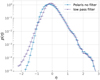 |
Fig. 5 η-PDFs. Blue round and purple triangular symbols represent the PDFs of the unflltered and low pass filtered maps, respectively. The filter does not alter regions with η > 0 but increases the occurrence of regions with η < −1. Horizontal errorbars represent bin spacing. |
6.4 Ergodic Estimate of the Observed PDF, Real Error Bars, and Reduced Integration Artifacts
As mentioned earlier, column-density PDFs serve as tracers of the statistics of the underlying density field. The various forms of these PDFs can be attributed to the various processes that are operating in MCs, from a fully lognormal distribution when purely turbulent motions dominate to a lognormal distribution with high density PLTs when gravitational effects become significant (Vazquez-Semadeni 1994; Passot & Vázquez-Semadeni 1998; Kainulainen et al. 2009; Schneider et al. 2013). This calls for a precise determination of the statistical uncertainty on the observed PDF, especially at high-density values.
The empirical PDF  of stochastic field X (here X will be the column density ŋ) is deduced from histograms with some bin size ∆ξ. Error bars are usually estimated from Poisson statistics (using the number of points per bin) and can therefore be very small (Schneider et al. 2013). It is worth delving deeper into this issue. A histogram yields the following estimate:
 (72)
(72)
where  is the empirical cumulative distribution function. Formally, this amounts to the ergodic estimate of the average of the following field, noted gξ0(y):
 (73)
(73)

(see Sect. 2.1.2 and 4). Thus, proper statistical error levels must be calculated using the results of Sect. 2 and in general are not given by Poisson statistics.
In Appendix B.2, we study in detail ergodic estimates of average quantities. In general, the correlation length of gξ0 is a function of ξ0itself. For Gaussian (or lognormal) distributions, an important result is that the confidence interval becomes quite large for values  , resulting in large errors if the sample size is too small. Thus, a reliable evaluation of the statistics of rare events (away from the average) requires very large sample sizes.
6.4.1 Reduced Integration Effects at High Density Contrasts
In this study, we focus on the column-density field X = ŋ and its PDF, noted p(ŋ). Using gŋ0(y) and its ACF for various values η0, we are able to determine the appropriate statistical error bars and to get rid of some of the artifacts that are due to integration along the line of sight. In practice, we expect that such artifacts are not significant in high column-density regions (see Sect. 6.2). For example, anisotropy of the Polaris column density ACF in the x-direction is likely due to integration effects (see Sect. 6.3).
We expect, however, that the ACF of field gŋ0 for ŋ0 > 0 is expected to show a reduced anisotropy at short scales. We thus obtain an empirical ACF of gŋ0 using Eq. (17). Figure 8 displays the estimated PDF of gŋ0 for the low pass filtered column-density map. At low column-density (η0 = −1.06), a strong anisotropy is observed in the x-direction starting at x/L ≥2× 10⁻², as for the ACF of ŋ (see Fig. 7). For positive column density contrasts (η0 > 0), this anisotropy is reduced and the ACFs are fairly isotropic at small scales in both the x and θ = π/4 directions, up to x/L ~ 10–1 and r/L ~ 10–1, respectively, where r denotes separation distance in the θ = π/4 direction. At larger separation distances, the data become quite noisy. This is consistent with the fact that the low path filtering procedure does not modify the PDF significantly in regions where ŋ > 0 (see Fig. 5).
This suggests that most of the ŋ ACF anisotropy in the x-direction at scales in the 10–2−10–1 range is due to integration effects. The peak of the correlation in the π/4-direction at high column-densities (ŋ0 = 1.58) is probably due to the presence of the “Saxophone”-shaped filamentary structure that may be seen at the top of Fig. 3, which hosts most of the Polaris high density regions (Schneider et al. 2013).
6.4.2 Statistical Errorbars
Using the statistics of ɡŋ0(y) has several advantages. One is that it reduces the impact of l.o.s. integration artifacts. In addition, it leads to proper error estimates for the empirical PDF.
Introducing some function of ŋ0 noted ϕ(ŋ0) which is expected to increase for increasing values of |ŋ0|, the confidence interval above (1 − 1/m2) can be written as follows (see Bienayme-Tchebychev inequality, Eq. (21)):
 (75)
(75)
with D = 2 and where
 (76)
(76)
 (77)
(77)
because  and where lc(ɡη0)2 ∝ Δη; so that the error bars on the PDF do not depend on the choice of bin size (for small Δη, see Appendix B.2).
From the empirical ACF  , one can then estimate the correlation length of ɡŋ0 and thus ϕ(ŋ0) for every ŋ0. Unfortunately, this procedure is hampered by the fact that the ACF becomes increasingly noisy at high contrasts |η0| > 1, due to sample sizes that are too small.
In principle, to determine ϕ(ŋ0) and its variation one must calculate the complete integral that defines lc(ɡŋ0). This may be avoided as follows. The growth of ϕ(ŋ0) may be obtained by looking at the short scale behavior of the ACFs of ɡŋ0. In Fig. 8, it appears that the values of  for positive column density contrasts (ŋ > 0) are isotropic and close to being ∝ |y|–1/2 at short scales. We thus write that:
 (78)
(78)
where  is a constant of proportionality that depends on ŋ0. Values of
  as a function of ŋ0 are given in Fig. 9. We have only studied ɡŋ0 for −0.7 ≤ ŋ0 ≤ 1.58, because the ACFs are extremely noisy at high positive density contrasts (ŋ ≥ 1.58) due to poor sampling. At negative density contrasts (ŋ ≤ −0.7), where integration artifacts are the largest (see Sect. 6.4.1), the ACFs are no longer sufficiently isotropic and do not conform to a scaling in |y|–1/2. Figure 9 shows that
  is an increasing function of |η0| for large |η0|, illustrating the fact that ϕ(ŋ0) is expected to be large compared to fŋ(ŋ0) for large contrasts |η0| > 1.
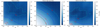 |
Fig. 6 Reduced ACF function of |

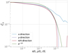 |
Fig. 7 Reduced ACF of the low pass Altered map in three different directions. Blue line: x-direction (y = 0). Purple line: y-direction (x = 0). Red line: π/4 or x = y-direction. Green line: exponential pro Ale giving an estimate of the rate of decay (here λ/L 5 × 10⁻²). A strong anisotropy is present in the x direction at large scales (x/L ≥ 2 × 10⁻²). |
6.4.3 Correlation Length of ɡη0 from Eq. (40)
To obtain an estimate of lc(ɡŋ0) and thus of ϕ(ŋ0), we can use the results of Sect. 3. For each ŋ0 we compute the field ɡη0(x, y) from the column density map ŋ(x, y). We then produce the two fields  and
and  obtained from the integration of ɡη0(x, y) along the x and y direction, respectively:
 (79)
(79)
 (80)
(80)
Computing the variance of these integrated fields we can obtain with Eq. (40) two estimates  and
and  of lc(ɡŋ0) within a factor of order unity:
 (81)
(81)
 (82)
(82)
where LX,y = 2RX,y are the lengths of the column density map in the x and y directions. For the present map of Polaris these two lengths are approximately equal, Lx ≃ Ly = L.
As, for ŋ0 > 0, the experimental ACFs of ɡŋ0 are fairly isotropic, we expect the above estimates of lc(ɡŋ0)/R (Eqs. (81) and (82)) to give similar and accurate results. They are given in Fig. 10 for Δη = 0.1 and always yield the same order of magnitude.
To test the accuracy of the estimates  and
and  of lc(ɡŋ0), we have tested how they scale with bin size Δη. If they were accurate estimates, they would have to conform to a scaling
  so that the error bars on the PDF (Eq. (75)) do not depend on the choice of bin size (see Appendix B.2). At positive density contrasts, ŋ > 0, the estimates
  and
and  follow a scaling close to the predicted
  . They do not, however, for negative contrasts, ŋ < 0, where the ACF is no longer isotropic and where there are strong integration artifacts. This can be seen on Fig. 11 where we display the shadded regions bounded by the two estimates
  and
and  for different bin sizes Δη at 4 values of η0 = −1.1,0.7, 1.1, 1.6.
We then conclude that  and
and  can be used to accurately estimate lc(ɡŋ0) for ŋ > 0, i.e. in the regions of interest for star formation. In practice we should assume that lc(ɡŋ0) lies somewhere between
  and
and  and compute error bars with both values. This is done in the next section.
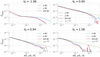 |
Fig. 8 Estimated ACF of the field ɡη0(y) for different values of ŋ0 = ŋ in 3 different directions. Blue, purple and red lines represent respectively the x, y and π/4 (x = y) directions. Two top panels are for ŋ0 = −1.06 and 0.69, whereas the two bottom panels are for ŋ0 = 0.94 and 1.58. At low column-densities (η0 = −1.06), a strong anisotropy is detected in the x-direction and becomes noticeable at x/L ≥ 2 × 10⁻² as was the case for the column-density ACF (see Fig. 7). For high column-densities (η0 > 0), however, the anisotropy is subdued and the ACFs are fairly isotropic at small scales up to x/L, r/L ~ 10–1 where the data become quite noisy. Green dashed lines show the profile of an isotropic ACF proportional to r–1/2 that matches the data at short scales fairly well, at least over a decade. |
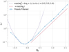 |
Fig. 9 Constant of proportionality |


 |
Fig. 10 Estimate of the ratio lc(ɡη0)/R from Eqs. (81) and (82) at different η0 for Δη = 0.1. The blue line gives the values of estimate |


 |
Fig. 11 Shadded regions bounded by the two estimates |


6.4.4 Effective Error Bars on the Observed PDF
Once we have obtained these estimates of lc(ɡŋ0)/R and tested their accuracy, we can compute effective error-bars at a given confidence interval for the PDF p(ŋo) = fŋ(ŋo) with Bienayme-Tchebychev inequality, Eq. (21):
 (83)
(83)
with  the estimate of the PDF produced by histograms of bin size Δη and m giving a confidence interval of over 1 − 1/m2.
Figure 12 displays the empirical Polaris PDF, with error bars computed from Eq. (83) for the two estimates  and
and  with Δη = 0.1. We have taken m = 2 to obtain a confidence interval of over 75%. As expected, the amplitudes of the error bars and thus of ϕ(ŋ0) grow with increasing values of |ŋ0|. These error bars may be inaccurate for ŋ0 < 0 because the estimates
  and
and  show a dependence that is too strong on bin size Δη at these low column densities (see Sect. 6.4.3). However, they are accurate at high column densities ŋ0 > 0 and serve to emphasize that error bars should not be derived from Poisson statistics and that the accuracy of the low and high end parts of the PDF are severely degraded by sample sizes that are too small.
7 Applications to the Orion B Cloud
In this section, we apply the results of Sect. 2 to the Orion B cloud (Schneider et al. 2013; Orkisz et al. 2017), another well studied star-forming MC. In this case, one encounters additional difficulties because the observed field is markedly elongated in the “vertical” direction (y) with data over a region whose geometrical shape is not suited to a straightforward data analysis (see Fig. 13). For this reason, we have extracted 2 parts of the cloud with rectangular shapes. One is elongated with a length that is close to the vertical dimension (Ly) of the total field of observation, which we shall refer to as a “filament”. A second part is a rectangular one with an aspect ratio close to 1, with a length close to the maximum horizontal length of the full cloud (Lx), which we shall refer to as a “square” region (see Fig. 13). We determine the ACF of these two subregions and the associated correlation lengths in Appendix C.
Using the ACF, we find that lc(ŋ)/Lx ~ 10–1. When using the variances Var (ρ) and Var (∑), we obtain a lower value: lc(ŋ)/Lz ~ 10–2, where Lz is the characteristic thickness of the cloud (along the line of sight).
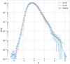 |
Fig. 12 PDF of the logarithmic column-density ŋ with statistical error-bars for m = 2 and the two estimates |


8 Conclusion
In this article, we have examined the validity of statistical homogeneity and ergodicity when deriving general properties of star-forming molecular clouds from observations or numerical results of some of their properties. Notably, we have focused on the field of density fluctuations and its PDF. This is a fundamental quantity since these fluctuations are believed to be at the root of the star formation process. It is thus essential to examine the validity of a statistical approach in order to assess the accuracy of the determination of the statistical properties of the cloud from the observations or simulations of a limited number of samples. To fulfill this goal, we first use the ergodic theory for any random field X to derive some rigorous statistical results. We explain how to calculate the correlation length of fluctuations in this field, lc(X), from the autocovariance function (ACF) (Eq. (11)). We show that the estimation of the correlation length allows one to define an effective number of samples, N, such that a space (or time) average of a single realization is formally equivalent to averaging over N independent samples (see e.g. Papoulis & Pillai 1965). When it is difficult to determine the correlation length from the empirical ACF, we have shown alternative ways to estimate it from fluctuations in Sect. 3.
We then apply this statistical approach and the results of ergodic theory to astrophysical systems in Sects. 4–6. In Sect. 4, we examine in particular the stochastic fields induced by compressible turbulent motions driven at large scale. We show that while the energy of turbulent motion is injected at large scale, comparable to the whole system L, the correlation length of either the specific kinetic energy or the density is actually small compared to L (see Sect. 4.3). We stress that there is no contradiction in these results since the injection scale and correlation length are two completely different quantities.
In Sect. 5 we apply our results to the observed column-density field, which is related to the (volume) density field in the cloud. Applying the results of Sect. 3, we have devised a method to determine the correlation length, or more exactly the ratio of the correlation length over the size of the cloud (or the box of numerical simulations), from the variances of both the volume-density and column-density fields. We have also shown that the statistics of the column-density field are affected by artifacts due to integration along the line of sight. These artifacts tend to generate an artificial anistropy in the colum density field and thus in the empirical ACF. Using the previous results, we have then examined in detail the Polaris cloud, which serves as a template for initial stages of star formation in MCs, in Sect. 6. We showed that the artificial anistropy in the empirical ACF results in an overestimation of the correlation length of density fluctuations within the cloud. Estimating the variance of the underlying density field, Var(ρ/ 〈ρ〉), and computing the variance of the column-density field, Var (∑/ 〈∑〉), we are able to derive a more accurate estimate of the correlation length lc (Eq. (63)), which can be an order of magnitude smaller than the one obtained from the empirical ACF (Sect. 6.3).
Moreover, we have shown that studying the statistics of the PDF ergodic estimator for positive column-density contrasts enables us to get rid of most of the integration anisotropy bias (Sect. 6.4.1). It also allows a proper evaluation of statistical error bars and shows that these (i) cannot be derived from simple Poisson statistics and (ii) become increasingly large for increasing density contrasts (|η| ≥ 1), severely reducing, in particular, the accuracy of the high end part of the PDF because of the small sample size (see Sect. 6.4.2). Furthermore, we provide a method that can be used by observers and numericists to determine robust error bars in Sect. 6.4.4.
Finally, we found that the correlation length of the density field in the Polaris cloud is of about ~1% of the size of the cloud (lc(ρ)/R ~ 10–2). We have also examined the more complex Orion B cloud to confirm the results obtained for Polaris in Sect. 7.
These calculations provide a rigorous framework for the analysis of the global properties of star-forming clouds from limited statistical observations of their density and surface fluctuating properties. They show in particular that for typical star-forming clouds at the onset of the star formation process, the correlation length of density fluctuations is much smaller than the size of the cloud. This justifies the assumption and the relevance of a statistical approach based on statistical homogeneity when studying the PDF of the cloud (Jaupart & Chabrier 2020, 2021), as done e.g. in cosmology or in the study of turbulence.
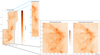 |
Fig. 13 Column-density maps of the Polaris cloud. Left panel: full observed field. Middle panel: extracted filamentary region. Right panel: extracted “square” region, unfiltered and low pass filtered (see Sect. 6). |
Acknowledgements
The authors are grateful to Christoph Federrath for always providing data from his numerical simulations upon request. This research has made use of data from the Herschel Gould Belt survey (HGBS) project (http://gouldbelt-herschel.cea.fr). The HGBS is a Herschel Key Programme jointly carried out by SPIRE Specialist Astronomy Group 3 (SAG 3), scientists of several institutes in the PACS Consortium (CEA Saclay, INAF-IFSI Rome and INAF-Arcetri, KU Leuven, MPIA Heidelberg), and scientists of the Herschel Science Center (HSC).
Appendix A Ergodic Estimate for a General Control Volume Ω
We described in Sec. (2) some known ergodic results, but they are derived for a cubic control volume ![${\rm{\Omega = }}{\left[ { - {L \over 2},{L \over 2}} \right]^D}$](/articles/aa/full_html/2022/07/aa41084-21/aa41084-21-eq201.png) . These results obviously do not depend on the shape of the control volume. We give here the general formulation for any control volume Ω possessing a center of symmetry (meaning that ∀y ϵ Ω, −y ϵ Ω). We again denote |Ω| the volume of Ω and define the linear size of Ω as LD = |Ω|. The ergodic estimate Eq. (4) is then
. These results obviously do not depend on the shape of the control volume. We give here the general formulation for any control volume Ω possessing a center of symmetry (meaning that ∀y ϵ Ω, −y ϵ Ω). We again denote |Ω| the volume of Ω and define the linear size of Ω as LD = |Ω|. The ergodic estimate Eq. (4) is then
 (A.1)
(A.1)
To obtain its variance, one has to compute the double integral
 (A.2)
(A.2)
Using the change of variables (u, v) = ϕ(y, z) = (y − z, y + z), one obtain
 (A.3)
(A.3)


We then obtain the general Slutsky’s theorem, X is mean ergodic if and only if
 (A.6)
(A.6)
Appendix B Ergodic Estimators of the CMF and PDF
Appendix B.1 Cumulative Distribution Function (CMF)
The CMF of the stochastic field X can be constructed as the average of a particular function of the field X. Indeed, by definition, FX(x0) = ℙ (X(y) ≤ x0) and a simple calculation shows that  with
with  , where Θ is Heaviside step function. We are then ready to determine the confidence interval for the estimated CMF FX of X. To do so, we need to apply the results of Sec. (2) to the field
  . The “natural” ergodic estimator of FX(x0) is thus:
![${\hat F_L}\left( {{x_0}} \right) = {1 \over {{L^D}}}\int_{{{\left[ { - {L \over 2},{L \over 2}} \right]}^D}} {{h_{{x_0}}}} \left( {X\left( {\bf{y}} \right)} \right){\rm{d}}{\bf{y}}.$](/articles/aa/full_html/2022/07/aa41084-21/aa41084-21-eq211.png) (B.1)
(B.1)
Then, to obtain the variance of  we need to express the ACF of
  (X(y)). We have
 (B.2)
(B.2)
where  and X(u) ≤ x0) is the second-order distribution function and is the probability to have both X(u + y) ≤ x0 and X(u) ≤ x0. The variance of
  is then
![${\rm{Var}}\left( {{{\hat F}_L}\left( {{x_0}} \right)} \right) = {1 \over {{{\left( L \right)}^D}}}\int_{{{\left[ { - L,L} \right]}^D}} {{C_{{h_{{x_0}}}}}} \left( {\bf{y}} \right)\prod\limits_{k = 1}^D {\left( {1 - {{|{y_k}|} \over L}} \right)} {\rm{d}}{\bf{y}}$](/articles/aa/full_html/2022/07/aa41084-21/aa41084-21-eq217.png) (B.3)
(B.3)
 (B.4)
(B.4)
providing  is integrable so one can define
  . Again, comparing with the result for a repeated trial experiment where N samples of X(y) are drawn (for the same point y) shows that the ratio
  serves as an effective number N of trials (see e.g. Papoulis & Pillai 1965).
For practical purpose and in order to give an interval of confidence, when FX is not known one can use the estimate  in Eq. (B.4) (Papoulis & Pillai 1965). Furthermore, here,
  is a function of x0 and cannot in general be simply estimated from lc(X). The length
  can, however, be estimated by repeating the experiment several times and using the results of Sec. (3.1).
Appendix B.2 Probability Density Function (PDF)
To build an estimator of the PDF fX(x0) of X we do not use the definition  but the common approximation, suited for data analysis,
  for a sufficiently small bin spacing Δx. Noting
  we build the estimator
![${\hat f_L}\left( {{x_0}} \right){\rm{\Delta }}x = {1 \over {{L^D}}}\int_{{{\left[ { - {L \over 2},{L \over 2}} \right]}^D}} {{g_{{x_0}}}} \left( {X\left( {\bf{y}} \right)} \right){\rm{d}}{\bf{y}}.$](/articles/aa/full_html/2022/07/aa41084-21/aa41084-21-eq228.png) (B.5)
(B.5)


We then know that a sufficient condition for X to be density ergodic is either  or
or  is integrable.
To find out how rapidly  decays to zero we note that
 (B.9)
(B.9)
 (B.10)
where  is the second-order density function. Eqs. B.9 and B.10 are only valid for y + 0 because
  is degenerate for
  , where min(x1, x2) is not differentiable. The variance of the ergodic estimator
  is, then,
 (B.11)
where  (see Eq. (B.10)).
Appendix B.3 Gaussian Process
If the field X(y) is Gaussian we have
 (B.12)
where xµ = (x1 − µ, x2 − µ), with  is the determinant of the matrix
  and
and
 (B.13)
We see that, as  is degenerate for y = 0. However, for y ≠ 0, we have
 (B.14)
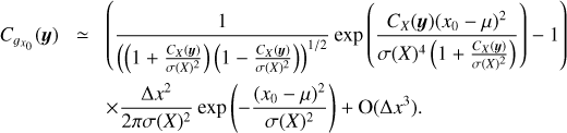
Noting the normalized ACF  and the reduced variable
  we have
 (B.16)
 (B.17)
Appendix B.3.1 Integrability of the ACF and Short Scale Analysis
If CX decays to zero (as assumed) then for |y| → ∞, we have  . Thus, if CX is integrable, then so is
  at |y| → ∞.
As mentioned above, Eq. (B.17) is only valid for |y| > 0, so the divergence at y = 0 is artificial as  is finite. However, if Eq. (B.17) is integrable at y = 0, this ensures that the errors of approximation of
  near y = 0 have a small effect on the estimation of
  (which is an integral). The divergence of Eq. (B.17) at y = 0 is given by
 (B.18)
For an exponential isotropic ACF this yields a divergence ∝ r–1/2, while for a differentiable field X with an ACF being isotropic at short scales this yields a divergence ∝ r–1. Thus, in most cases for D ≥ 2 Eq. (B.17) is integrable at |y| → 0.
Computing the integral of  is not straightforward for any decaying and integrable ACF CX(y). Expanding the exponential in Eq. (B.17), we have
 (B.19)
We then have to specify or bound the integrals
 (B.20)
 (B.21)

where  is a function of x0 which we need to bound to obtain a confidence interval. A lower bound of
  can be obtained due to the convexity of the exponential:
 (B.23)
For general monotonic decreasing (hence positive) ACFs, the study of the functions  and
and  shows that C0 ≳ 0.1 and c1 ≥ 0.77.
Appendix B.3.2 Exponential ACF
To go a little further and obtain a formula that will help to grasp some expected features of the ergodic estimate of  we study the special case of an exponential ACF. For the present study we limit ourselves to the case D ≤ 2. Then if
  is an (isotropic) exponential,
  , we can bound the integral of Eq. (B.17). Indeed, for n ≥ 1,
 (B.24)

where  and 0.17 for D = 1 and D = 2, respectively. This gives an upper bound to the correlation length of
  but overestimates its value for
  . However, near the average
  we can approximate
 (B.26)
where  and 0.88 for D = 1 and D = 2, respectively. We note that, due to the convexity of the exponential, the right hand side of Eq. (B.26) is actually a lower bound of the integral
  .
.
We can then construct a confidence interval with more than 1 − 1/m2 of confidence such that the true fX(x0) lies in


Using the lower bound to approximate  while accurate for
  , is most probably an underestimation for
  . However, it allows to show that the statistics of events that deviate largely from the mean needs an increasingly large sample size to have a high degree of confidence.
Appendix B.4 Deterministic Function of a Gaussian Field
The results derived in Sec. (B.3) can be extended to the case where X(y) = ψ(S (y)) with ψ a diffeomorphism and S a Gaussian field. A particular example is that of a lognormal field where ψ = exp. We call this function ψ a deterministic function because statistical properties of the field X can be obtained from those of S. Indeed, for such a field X, the first and second order distribution functions read
 (B.28)
 (B.29)
where Sj = ψ–1(xj) (Papoulis & Pillai 1965). Without loss of generality we can further assume that the field S is centered with variance unity. We note that the function ψ can be obtained by inverting Eq. (B.28). Indeed, if only fX and fS are known we can obtain ψ by realizing that ψ–1 verifies the differential equation:
 (B.30)
If one further assumes that ψ is an increasing diffeomorphism (ψ–1)′ ≥ 0, one obtains
 (B.31)
where xmin is the minimum value that can be taken by the field X and erf–1 is the inverse of the error function. The use of this equation requires a high precision on fX due to the large variation of erf–1 , which is complicated in general.
Then the ACF of X can be obtained by performing the integral:

Then Eq. (B.17) becomes
 (B.32)
Appendix B.4.1 Log-normal Fields
For a log-normal field ρ = exp(s), ψ = exp, ψ–1 = ln and s is not centered  and does not have a variance unity (σ(s) ≠ 1), in general. Then the calculation of the ACF yields:
 (B.33)
As a consequence, because eax − 1 ≤ x(ea − 1) for 0 ≤ x ≤ 1 and ax ≤ eax − 1 ∀x, if Cρ (or Cs) is monotonically decaying to 0 then
 (B.34)
In typical star forming conditions σ(s)2 ≲ 4, giving
 (B.35)

This suggests that as long as Var (X) = Var (ψ(S)) is not too big, one can expect to have lc(X) ~ lc(S).
Appendix C Orion B Cloud
Appendix C.1 ACF of the Square and Filament Region
We computed the ACF of the unfiltered and low pass filtered square region (up to scale L/2, see §6), as well as the (unfiltered) “filament” region. The results are presented in Figs. (C.1) and (C.2). Filtering large-scale gradients reduces again the anisotropy at short scales and reduces the estimated correlation length.
To have a closer look at the behavior of the ACF of Orion B, we display in Fig. (C.3) the reduced ACF of the low pass filtered map in 3 different directions, x (θ = 0), x = y (θ = π/4) and y (θ = π/2). As seen from the heat maps but also from fig. (C.3), a strong anisotropy is present and located in the y direction at large scales (y/L ≥ 10–1). The resulting estimated correlation length  is of the order lc(η)/Lx ≃ 10–1.
 |
Fig. C.1 ACF of the “square region”. Left panel: unflltered. Right panel: low pass filtered up to scale L/2. Again, filtering large-scale gradients reduces the anisotropy at short scales and reduces the estimated correlation length. |
Appendix C.2 Correlation Length from the Variance of the Column Densities
As seen from Sec. (5.2) and Eq. (63), one can also give an estimate of the ratio lc(ρ)/R by (1) computing the variance Var  , (2) giving an estimate of Var
  and (3) giving an estimate of the average thickness of the cloud (along the line of sight) Lz. Here Orion B appears as a very elongated structure, and we will therefore only assume that Ly ≥ Lz ≳ Lx (with Ly ≃ 3 - 4 Lx).
From observations of column densities we obtain Var(∑/ 〈∑〉) ≃ 1.1 while the PDF of column densities, exhibiting a power-law tail of exponent αη = −2 (Schneider et al. 2013; Jaupart & Chabrier 2020), indicates an underlying density PDF with a power-law tail of exponent −3/2 implying a large variance. As For Polaris, running the power-law tail from s = 8 to s = sad ≃ 16 yields a variance Var  and Var
  respectively (see Jaupart & Chabrier 2020). This yields a ratio lc(ρ)/Lz ≲ 10–2.
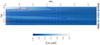 |
Fig. C.2 ACF of the unflltered “filament region”. A strong anisotropy is present in the y-direction. |
 |
Fig. C.3 Reduced ACF of the low pass filtered map in three different directions. Red line: x-direction (y = 0). Blue line: y-direction (x = 0). Green line: π/4 or x = y-direction. Dash dotted lines represent the values of the ACF when it is negative. A strong anisotropy is present in the y direction at large scales (y/L ≥ 10–1). |
References
- Alves, J., Lombardi, M., & Lada, C. J. 2017, A&A, 606, L2 [NASA ADS] [CrossRef] [EDP Sciences] [Google Scholar]
- André, P., Men’shchikov, A., Bontemps, S., et al. 2010, A&A, 518, L102 [CrossRef] [EDP Sciences] [Google Scholar]
- Batchelor, G. K. 1953, The Theory of Homogeneous Turbulence (Cambridge: Cambridge University Press) [Google Scholar]
- Beaulieu, N. C. 2011, IEEE Trans. Commun., 60 23 [Google Scholar]
- Brunt, C., Heyer, M., & Mac Low, M.-M. 2009, A&A, 504 883 [NASA ADS] [CrossRef] [EDP Sciences] [Google Scholar]
- Brunt, C. M., Federrath, C., & Price, D. J. 2010, MNRAS, 403 1507 [Google Scholar]
- Chandrasekhar, S. 1951a, Proc. R. Soc. London Ser. A. Math. Phys. Sci., 210 18 [NASA ADS] [Google Scholar]
- Chandrasekhar, S. 1951b, Proc. R. Soc. London Ser. A Math. Phys. Sci., 210 26 [NASA ADS] [Google Scholar]
- Federrath, C. 2013, MNRAS, 436 1245 [NASA ADS] [CrossRef] [Google Scholar]
- Federrath, C. 2016, MNRAS, 457 375 [Google Scholar]
- Federrath, C., & Klessen, R. S. 2013, ApJ, 763 51 [Google Scholar]
- Federrath, C., Roman-Duval, J., Klessen, R., Schmidt, W., & Mac Low, M.-M. 2010, A&A, 512, A81 [NASA ADS] [CrossRef] [EDP Sciences] [Google Scholar]
- Frisch, U. 1995, Turbulence: the Legacy of AN Kolmogorov (Cambridge: Cambridge University Press) [CrossRef] [Google Scholar]
- Heinesen, A. 2020, J. Cosmol. Astropart. Phys., 2020 052 [CrossRef] [Google Scholar]
- Hennebelle, P., & Chabrier, G. 2008, ApJ, 684 395 [Google Scholar]
- Hopkins, P. F. 2012, MNRAS, 423 2037 [NASA ADS] [CrossRef] [Google Scholar]
- Jaupart, E., & Chabrier, G. 2020, ApJ, 903, L2 [NASA ADS] [CrossRef] [Google Scholar]
- Jaupart, E., & Chabrier, G. 2021, ApJ, 922, L36 [NASA ADS] [CrossRef] [Google Scholar]
- Kainulainen, J., Beuther, H., Henning, T., & Plume, R. 2009, A&A, 508, L35 [NASA ADS] [CrossRef] [EDP Sciences] [Google Scholar]
- Kleiner, S., & Dickman, R. 1984, ApJ, 286 255 [NASA ADS] [CrossRef] [Google Scholar]
- Kleiner, S., & Dickman, R. 1985, ApJ, 295 466 [NASA ADS] [CrossRef] [Google Scholar]
- Kritsuk, A. G., Norman, M. L., Padoan, P., & Wagner, R. 2007, ApJ, 665 416 [NASA ADS] [CrossRef] [Google Scholar]
- Mac Low, M.-M., & Klessen, R. S. 2004, Rev. Mod. Phys., 76 125 [Google Scholar]
- Machida, M. N., Inutsuka, S.-I., & Matsumoto, T. 2006, ApJ, 647, L151 [NASA ADS] [CrossRef] [Google Scholar]
- Masunaga, H., & Inutsuka, S.-I. 2000, ApJ, 531 350 [NASA ADS] [CrossRef] [Google Scholar]
- McKee, C. F., & Ostriker, E. C. 2007, ARA&A, 45 565 [Google Scholar]
- Miville-Deschênes, M.-A., Martin, P., Abergel, A., et al. 2010, A&A, 518, L104 [NASA ADS] [CrossRef] [EDP Sciences] [Google Scholar]
- Orkisz, J. H., Pety, J., Gerin, M., et al. 2017, A&A, 599, A99 [NASA ADS] [CrossRef] [EDP Sciences] [Google Scholar]
- Ossenkopf-Okada, V., Csengeri, T., Schneider, N., Federrath, C., & Klessen, R. S. 2016, A&A, 590, A104 [NASA ADS] [CrossRef] [EDP Sciences] [Google Scholar]
- Padoan, P., & Nordlund, Å. 2002, ApJ, 576 870 [NASA ADS] [CrossRef] [Google Scholar]
- Pan, L., Padoan, P., & Nordlund, Å. 2018, ApJ, 866, L17 [NASA ADS] [CrossRef] [Google Scholar]
- Pan, L., Padoan, P., & Nordlund, Å. 2019a, ApJ, 876 90 [NASA ADS] [CrossRef] [Google Scholar]
- Pan, L., Padoan, P., & Nordlund, Å. 2019b, ApJ, 881 155 [NASA ADS] [CrossRef] [Google Scholar]
- Papoulis, A., & Pillai, S. 1965, Variables Stochastic Processes (New York: McGraw-Hill) [Google Scholar]
- Passot, T., & Vázquez-Semadeni, E. 1998, Phys. Rev. E, 58 4501 [Google Scholar]
- Peebles, P. J. E. 1973, ApJ, 185 413 [Google Scholar]
- Pope, S. B. 1985, Prog. Energy Combustion Sci., 11 119 [NASA ADS] [CrossRef] [Google Scholar]
- Reinke, N., Fuchs, A., Hölling, M., & Peinke, J. 2016, in Fractal Flow Design: How to Design Bespoke Turbulence and Why (Berlin: Springer), 165 [Google Scholar]
- Reinke, N., Fuchs, A., Nickelsen, D., & Peinke, J. 2018, J. Fluid Mech., 848 117 [NASA ADS] [CrossRef] [Google Scholar]
- Scalo, J. 1984, ApJ, 277 556 [NASA ADS] [CrossRef] [Google Scholar]
- Schneider, N., André, P., Könyves, V., et al. 2013, ApJ, 766, L17 [NASA ADS] [CrossRef] [Google Scholar]
- Schneider, N., Ossenkopf, V., Csengeri, T., et al. 2015, A&A, 575, A79 [CrossRef] [EDP Sciences] [Google Scholar]
- Szyszkowicz, S. S., & Yanikomeroglu, H. 2009, IEEE Trans. Commun., 57 3538 [CrossRef] [Google Scholar]
- Vaytet, N., Chabrier, G., Audit, E., et al. 2013, A&A, 557, A90 [NASA ADS] [CrossRef] [EDP Sciences] [Google Scholar]
- Vaytet, N., Commerçon, B., Masson, J., González, M., & Chabrier, G. 2018, A&A, 615, A5 [NASA ADS] [CrossRef] [EDP Sciences] [Google Scholar]
- Vazquez-Semadeni, E. 1994, ApJ, 423 681 [Google Scholar]
- Vázquez-Semadeni, E., & García, N. 2001, ApJ, 557 727 [CrossRef] [Google Scholar]
- Vázquez-Semadeni, E., Palau, A., Ballesteros-Paredes, J., Gómez, G. C., & Zamora-Avilés, M. 2019, MNRAS, 490 3061 [Google Scholar]
The following calculations are made with this particular type of cubic control volume, as the calculations are easier to follow. We give in Appendix A the calculations for a control volume of any shape.
If the statistics are Gaussian, we obtain an equality where we have 0.67 instead of  in Eq. (26).
All Figures
|
Fig. 1 Projection of the two idealized situation. Left panel: case of a sphere. Right panel: case of a cuboid mis-aligned with the line of sight. |
| In the text | |
|
Fig. 2 Column and volume density PDF of the Polaris cloud. Left: Observed logarithmic column-density (ŋ = ln(∑/ 〈∑〉)-PDF (Schneider et al. 2013; Jaupart & Chabrier 2020). Right: Estimated and reconstructed underlying logarithmic density |
| In the text | |
|
Fig. 3 Column-density maps of the Polaris cloud. Left panel: without filter. Middle panel: with a high-pass filter filtering scales smaller than L/2. Right panel: with a low pass filter filtering scales larger than L/2. The low pass filter does not alter qualitatively the richness of structures found in the Polaris flare, while the high-pass filter shows a large-scale gradient that can be produced by an integration effect. |
| In the text | |
|
Fig. 4 Same as Fig. (3), but for the binary map Θ(log(∑/ 〈∑〉))where Θ is Heaviside’s step function. Regions where ∑ > 〈∑〉 appear darker than regions where ∑ < 〈∑〉. |
| In the text | |
|
Fig. 5 η-PDFs. Blue round and purple triangular symbols represent the PDFs of the unflltered and low pass filtered maps, respectively. The filter does not alter regions with η > 0 but increases the occurrence of regions with η < −1. Horizontal errorbars represent bin spacing. |
| In the text | |
|
Fig. 6 Reduced ACF function of |
| In the text | |
|
Fig. 7 Reduced ACF of the low pass Altered map in three different directions. Blue line: x-direction (y = 0). Purple line: y-direction (x = 0). Red line: π/4 or x = y-direction. Green line: exponential pro Ale giving an estimate of the rate of decay (here λ/L 5 × 10⁻²). A strong anisotropy is present in the x direction at large scales (x/L ≥ 2 × 10⁻²). |
| In the text | |
|
Fig. 8 Estimated ACF of the field ɡη0(y) for different values of ŋ0 = ŋ in 3 different directions. Blue, purple and red lines represent respectively the x, y and π/4 (x = y) directions. Two top panels are for ŋ0 = −1.06 and 0.69, whereas the two bottom panels are for ŋ0 = 0.94 and 1.58. At low column-densities (η0 = −1.06), a strong anisotropy is detected in the x-direction and becomes noticeable at x/L ≥ 2 × 10⁻² as was the case for the column-density ACF (see Fig. 7). For high column-densities (η0 > 0), however, the anisotropy is subdued and the ACFs are fairly isotropic at small scales up to x/L, r/L ~ 10–1 where the data become quite noisy. Green dashed lines show the profile of an isotropic ACF proportional to r–1/2 that matches the data at short scales fairly well, at least over a decade. |
| In the text | |
|
Fig. 9 Constant of proportionality |
| In the text | |
|
Fig. 10 Estimate of the ratio lc(ɡη0)/R from Eqs. (81) and (82) at different η0 for Δη = 0.1. The blue line gives the values of estimate |
| In the text | |
|
Fig. 11 Shadded regions bounded by the two estimates |
| In the text | |
|
Fig. 12 PDF of the logarithmic column-density ŋ with statistical error-bars for m = 2 and the two estimates |
| In the text | |
|
Fig. 13 Column-density maps of the Polaris cloud. Left panel: full observed field. Middle panel: extracted filamentary region. Right panel: extracted “square” region, unfiltered and low pass filtered (see Sect. 6). |
| In the text | |
|
Fig. C.1 ACF of the “square region”. Left panel: unflltered. Right panel: low pass filtered up to scale L/2. Again, filtering large-scale gradients reduces the anisotropy at short scales and reduces the estimated correlation length. |
| In the text | |
|
Fig. C.2 ACF of the unflltered “filament region”. A strong anisotropy is present in the y-direction. |
| In the text | |
|
Fig. C.3 Reduced ACF of the low pass filtered map in three different directions. Red line: x-direction (y = 0). Blue line: y-direction (x = 0). Green line: π/4 or x = y-direction. Dash dotted lines represent the values of the ACF when it is negative. A strong anisotropy is present in the y direction at large scales (y/L ≥ 10–1). |
| In the text | |
Current usage metrics show cumulative count of Article Views (full-text article views including HTML views, PDF and ePub downloads, according to the available data) and Abstracts Views on Vision4Press platform.
Data correspond to usage on the plateform after 2015. The current usage metrics is available 48-96 hours after online publication and is updated daily on week days.
Initial download of the metrics may take a while.