© The Authors 2023

1 Introduction

High-contrast extreme adaptive optics (AO) systems such as SPHERE (Spectro-Polarimetry High-contrast Exoplanet REsearch; Beuzit et al. 2019), GPI (Gemini Planet Imager; Macintosh et al. 2006, 2014), or SCExAO (Jovanovic et al. 2015) have been developed to directly observe the close environment of stars in the visible and the near-infrared. The study of exoplan-ets and their formation is among the main scientific objectives of these instruments. One of the advantages of high-contrast extreme AO systems is that they can provide direct access to the light from the exoplanet, which is crucial when performing spectral characterizations. However, substantial contamination by the light from the host star occurs: in the visible and the near-infrared, in spite of the real-time correction by the AO system and of the masking of the host star by a coronagraph, the residual stellar light diffracted by the instrument is much brighter than that received from most exoplanets of interest. For this reason, dedicated post-processing methods have been developed to track evidence of the presence of exoplanets in data corrupted by strong stellar leakages. The number of published detection algorithms, LOCI (Lafreniere et al. 2007), TLOCI (Marois et al. 2013), KLIP (Soummer et al. 2012), MOODS (Smith et al. 2009), ANDROMEDA (Mugnier et al. 2009), PEX (Devaney & Thiébaut 2017), and PACO (Flasseur et al. 2018, 2020a,b), to name a few, reflects the scientific interest but also the intrinsic difficulty of trustfully detecting an exoplanet from sequences of high-contrast images. The most successful of these methods are those that account for the statistics of the stellar leakages (notably their correlations), no matter if they consist of sequences of images (Smith et al. 2009; Flasseur et al. 2018, 2020b), sequences of multi-spectral images from Integral field spectrographs (IFS; Flasseur et al. 2020a), or even multi-epoch sequences of images (Dallant et al. 2022).

After its detection, the direct characterization of an exo-planet is possible with high-contrast extreme AO systems equipped with a spectrograph. Both SPHERE and GPI are equipped with low-resolution IFS. In addition, SPHERE/IRDIS is equipped with a medium (MRS) resolution long-slit spectro-graph (LSS) in J, H, and K bands, with the latter being also available at low (LRS) resolution¹ (Dohlen et al. 2008). With SPHERE/IRDIS/LSS, the spectrum of a detected companion can then be measured by aligning the slit of the spectrograph with the host star and the companion while the host star is occulted by an opaque mask combined with the slit. In an LSS image, the stellar leakages take the form of speckles spectrally dispersed along oblique lines generally brighter than the companion spectrum (see Fig. 1 for an example). In order to get rid of these stellar leakages, Vigan et al. (2008, 2012) have developed a spectral deconvolution (SD) method following the work of Sparks & Ford (2002). The SD method consists of a filtering of the LSS image after a geometrical transform to align the speckles along a given direction. In practice, the SD method is quite sensitive to the alignment of the instrument, requires fixing defective pixels, and suffers from a self-subtraction bias. The latter is due to an overestimation of the stellar leakages caused by the presence of the companion. To improve on the SD method and reduce the self-subtraction bias, Mesa et al. (2016) adapted the strategy implemented in TLOCI (Marois et al. 2013) to the LSS data. In spite of these improvements, existing extraction methods suffer from a number of faults, most of them stemming from the requirement to geometrically transform the LSS data to align the dispersed speckles. In particular, they provide, at best, a least-squares estimation of the stellar leakages which is sub-optimal as the noise is not independent or identically distributed (i.i.d.) in the geometrically transformed images (Thiébaut et al. 2016). To overcome the drawbacks of existing methods, we propose formulating the extraction of the spectrum of a companion as an inverse problem. The inverse problem corresponds to the joint estimation of the contributions of the star and of its companion from the LSS data. Not only does this approach require no transformation of the LSS data (thus avoiding the introduction of correlations) but it also yields statistically optimal estimators. To cope with both the possible instrumental misalignment and the lack of a closed-form solution for the inverse problem, we implemented an alternating optimization strategy with optional self-calibration stages to solve the problem.

The outline of the paper is as follows. In Sect. 2, we present a model of the distribution of the light on the detector of a LSS instrument. This model is used to illustrate how (following a geometrical transform) stellar leakages can be partially removed by a truncated singular value decomposition (TSVD) before extracting the companion signal. Such an approach is representative of the optimal performance that can be reached by standard methods. We present in Sect. 3 our approach to jointly estimate the stellar leakages and the contribution of the companion without transforming the data. For the processing of LSS data, knowledge the spectro-angular coordinates of each detector pixel is requisite and we describe in Sect. 4 a numerical method to estimate the spatio-spectral dispersion laws from given calibration data. In Sect. 5, we validate the proposed method on both real data from SPHERE/IRDIS/MRS and on injections of synthetic companions in real data. We show the importance of the calibration (described in Appendix A) and compare our method with more standard approaches. Finally, we conclude in Sect. 6 and present some possible modifications of the proposed methods.

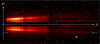Fig. 1 Long-slit medium resolution spectroscopy data of HR 3549 taken by IRDIS, with horizontally the spectral axis λ and vertically the angular separation axis, ρ. The blue arrows indicate the position of the companion.

2 State-of-the-art processing

In spite of the coronagraphic mask in high-contrast data, the stellar leakages, taking the form of quasi-static dispersed speckles, largely dominate the signal of interest, namely, the spectrum of the companion. These speckles, whose contribution cannot be precisely determined by using other stars (i.e., by reference differential imaging; Xie et al. 2022) or by rotating the slit to hide the planet (Vigan 2016) are a major source of nuisance for extracting the companion spectrum. This section introduces a modeling of the LSS data that is used in Sect. 3 to design our spectrum extraction method. This model is also useful to explain how previous approaches perform the suppression of the stellar leakages (Vigan et al. 2008; Mesa et al. 2016).

2.1 Image formation

Figure 1 shows a single exposure captured by the LSS of SPHERE/IRDIS. The vector d ∈ ℝ^N, with N the number of pixels, can be modeled by: $$d_n=m\left({\rho }_n,{\lambda }_n\right)+{\epsilon }_n,$$(1)

with m(ρ, λ) the distribution of light in the detector plane at an angular coordinate, ρ, along the slit and wavelength, λ and ρ_n, and λ_n as the angular and spectral coordinates at the nth pixel, and ɛ_n the contribution of the noise. Our notations are summarized in Table 1. The light distribution in the detector plane is the sum of the contributions by the star and by the companion: $$m\left(\rho ,\lambda \right)=f_{★}\left(\lambda \right)h_{★}\left(\rho ,\lambda \right)+f_{\oplus }\left(\lambda \right)h_{\oplus }\left(\rho ,\lambda \right),$$(2)

with f_⋆ and f_⊕ the spectral energy distributions (SEDs) of the star and of the companion as seen by the detector², h_⋆, and h_⊕ the point spread functions (PSFs) for a source at the respective angular positions of the star and of the companion, namely, the so-called on-axis and off-axis PSFs. The on-axis PSF, h_⋆(ρ, λ) explains the oblique bright lines due to stellar leakages in Fig. 1, while the stellar SED f_⋆(λ) explains the variations of intensity along these lines. As can be seen in Fig. 1, the companion signal, that is, f_⊕,(λ) h_⊕(ρ, λ), is barely distinguishable in the LSS data and it is mandatory to get rid of the stellar leakages f_⋆(λ) h_⋆(ρ, λ).

2.2 Low-rank approximation of the stellar leakages

Devaney & Thiébaut (2017) have shown that, except in the vicinity of the coronagraphic mask, the chromatic PSF can be written in the form of a series expansion. Applying their model to the star and taking into account that our data have one angular dimension instead of two yields: $$h_{★}\left(\rho ,\lambda \right)={\displaystyle {\sum }_{k\ge 1}\gamma {\left(\lambda \right)}^k{h}_{★}{{}_{,}}_k\left(\gamma \left(\lambda \right)\left(\rho -{\rho }_{★}\right)\right),}$$(3)

with γ(λ) = λ^ref/λ a chromatic magnification factor relative to some arbitrary reference wavelength λ^ref, ρ_⋆ the angular position of the star along the slit to account for a possible pointing error of the instrument, and [h_⋆,k}_k=ı,… a family of spatial PSF modes at the reference wavelength.

Since the stellar leakages dominate the signal in the LSS image, d, Eq. (3) suggests applying specific image warping so as to form a 2D image, d^warp, whose first dimension may vary along the wavelength, while its second dimension varies along the coordinate s = γ(λ) (ρ – ρ_⋆). For more details, we refer to Fig. 2. According to Eqs. (1) and (3), the warped image is modeled and then approximated by: $$d_{i,j}^{\text{warp}}=m\left({\rho }_{★}+s_j^{\text{warp}}/\gamma \left({\lambda }_i^{\text{warp}}\right),{\lambda }_i^{\text{warp}}\right)+{\epsilon }_{i,j}^{\text{warp}},$$(4) $$\approx {\displaystyle \sum _{k\ge 1}\gamma {\left({\lambda }_i^{\text{warp}}\right)}^k{f}_{★}\left({\lambda }_i^{\text{warp}}\right)h_{★,k}\left(s_j^{\text{warp}}\right),}$$(5)

where ɛ^warp in Eq. (4) denotes the contribution of the noise in the warped image while the ≈ symbol in Eq. (5) is to account for the contributions of the potential companion and for the noise which have been neglected. In other words, the stellar leakages appear to have a simple separable decomposition in the warped image.

The singular value decomposition (SVD) of the warped image³ is expressed as: $$d^{\text{warp}}={\displaystyle \sum _{k=1}^{\min \left(N_1,N_2\right)}{u}_k{\sigma }_k{\upsilon }_k^{\top },}$$(6)

where N₁ and N₂ are the dimensions of the warped image, $u_k\in {\text{ℝ}}^{N_1}$ is the kth left singular vector of the decomposition, σ_k ≥ 0 is the kth singular value, and ${\upsilon }_k\in {\text{ℝ}}^{N_2}$ is the kth right singular vector. Comparing Eq. (5) and Eq. (6), we see that the SVD of d^warp readily provides a decomposition similar to the contribution of the stellar leakages with, for each index, k, the left singular vector, u_k, sampling γ(λ)^k f_⋆(λ) as a function of λ and the right singular vector, υ_k, sampling h_⋆,k(s) as a function of s (both up to a normalization factor that depends on k). The truncated singular value decomposition (TSVD) of the warped image is obtained by limiting the sum in the right-hand side of Eq. (6) to the k_max ≤ min(N₁,N₂) first terms; also, according to the Eckart-Young-Mirsky (Eckart & Young 1936; Mirsky 1960) theorem, it is the best possible approximation of d^warp of rank k_max in the least-squares approach. Hence, it may be assumed that, for a suitable choice of k_max, the TSVD of d^warp provides a good approximation of the stellar leakages without being too much affected by the companion signal (if the companion is not too bright) and by the noise. A residual image that mostly depends on the companion can then be formed by subtracting the un-warped TSVD of the warped image d^warp from the LSS image d: $$r_{\oplus }=d-𝒰\left({\displaystyle \sum _{k=1}^{k_{\max }}{u}_k{\sigma }_k{\upsilon }_k^{\top }}\right),$$(7)

where 𝒰 denotes the un-warping operation⁴. As illustrated by Fig. 3, the signal of interest (i.e., the companion SED) is then easier to extract from the residual image, r_⊕. This can be done with standard aperture photometry tools.

As pointed out by Devaney & Thiébaut (2017), there are a number of issues in using the TSVD to get rid of the stellar leakages in multi-wavelengths high-contrast data. First, to produce a rectangular warped image (that can be interpreted as a matrix to perform the SVD), quite substantial regions of the original data, d, have to be discarded (i.e., those near the coronagraphic mask and the edges of the formed image). This limits the range of admissible angular positions for the companion and gets rid of data that might be valuable to improve the estimation of the stellar leakages. Second, the presence of a companion in the original data, d, yields a positive bias in the approximation of the stellar leakages by the TSVD. This results in a negative bias in the residual image and, hence, in the estimated companion SED. This artifact is known in the literature as “self-subtraction”. Third, the least-squares fit performed by the TSVD of d^warp is sub-optimal regarding the distribution of the noise in the warped image. Indeed, a least squares approach is only optimal for independent identically distributed (i.i.d.) noise, which is certainly not the case for ${\epsilon }_{i,j}^{\text{warp}}$: at least, the shot noise in the image, d has a non-uniform distribution and a side effect of the transform of d to yield the warped image, d^warp, is the introduction of correlations. Moreover, defective pixels, which are quite numerous for the kind of detectors used by NIR instruments such as LSS, must be corrected, usually by averaging their neighbors’ values, before warping the image. This correction can only introduce additional correlations.

In spite of these drawbacks, the proposed processing methods (Vigan et al. 2008; Mesa et al. 2016) are similar to the TSVD approximation of warped LSS images (optimal linear combination of a set of images). Some refinements have been proposed to limit the self-subtraction bias (Mesa et al. 2016) but the other issues have been largely left unaddressed. In the rest of this paper, we propose a new “inverse problems” approach to solve all the aforementioned limitations.

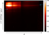Fig. 2 Warped HR 3549 image. This figure shows the bottom half of the data shown in Fig. 1, corresponding to the side where lies the companion, warped so as to align the dispersed speckles of the stellar leakages. The warping is defined by the coordinates ρ and λ of the pixels given by the “complex” calibration model of the spectral and angular dispersion laws described in Appendix A. The companion signal can be seen as a faint curved track indicated by the blue arrows.

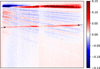Fig. 3 Bottom half of the residual image r⊕ for the HR 3549 data with stellar leakages estimated by the TSVD method as defined in Eq. (7) and with the warped image shown in Fig. 2. Compared to the original data shown in Fig. 1, the companion signal appears more distinctly (indicated by the two arrows).

3 Inverse problems approach

To avoid the issues resulting from warping the LSS image, we propose solving an inverse problem that consists of jointly estimating the parameters of the direct model of the data given in Eqs. (1) and (2) without transforming the data themselves. For an optimal information extraction, we model the likelihood of the data to consider the uneven quality of the data and, therefore, to account for defective pixels or missing data in a consistent way. Besides, our approach relies on a precise calibration of the spectro-spatial instrumental dispersion as seen by the detector. The proposed method includes auto-calibration stages to refine the calibration parameters and thus accounts for a possible misalignment of the science exposures.

3.1 Assumed continuous model

To simplify the on-axis PSF model in Eq. (3), we kept only the first and most significant of these modes. Thus we assume that: $$h_{★}\left(\rho ,\lambda \right)=\gamma \left(\lambda \right)h_{★}\left(\gamma \left(\lambda \right)\left(\rho -{\rho }_{★}\right)\right),$$(8)

with h_⋆(ρ) = h_⋆,1(ρ) as the first spatial mode of the on-axis PSF. As shown in Sect. 5, this simple model of the stellar leakages already gives excellent results. Likewise, the chromatic off-axis PSF h_⊕ can also be written as: $$h_{\oplus }\left(\rho ,\lambda \right)\approx \gamma \left(\lambda \right)h_{\oplus }\left(\gamma \left(\lambda \right)\left(\rho -{\rho }_{\oplus }\right)\right),$$(9)

with h_⊕(ρ) = h_⊕(ρ, λ^ref) the off-axis PSF at the reference wavelength λ^ref and ρ_⊕ the angular position of the companion along the slit. We note that the γ(λ) factor ensures that the on-axis and off-axis PSFs be normalized at all wavelengths provided the PSF at the reference wavelength be also normalized, namely, ∫h(ρ, λ)dρ = 1 (∀λ). These approximations for the on-axis and off-axis PSFs yield the following simplified model, presented in Fig. 4, that we assume for the rest of the paper: $$\begin{array}{l}m\left(\rho ,\lambda \right)=\gamma \left(\lambda \right)[f_{★}\left(\lambda \right)h_{★}\left(\gamma \left(\lambda \right)\left(\rho -{\rho }_{★}\right)\right)\hfill \\ +f_{\oplus }\left(\lambda \right)h_{\oplus }\left(\gamma \left(\lambda \right)\left(\rho -{\rho }_{\oplus }\right)\right)].\hfill \end{array}$$(10)

3.2 Discretized distribution

In order to fit the data, the model m(ρ, λ) in Eq. (10) has to be estimated at each angular and spectral coordinates (ρ_n, λ_n) of the N pixels of the detector. These pixel coordinates can be identified by fitting angular and spectral dispersion laws to calibration data, as explained in Appendix A. Because of these angular and spectral dispersion laws, continuous functions are needed to model the SEDs of the star and the companion (f_⋆ and f_⊕) and their respective PSFs (h_⋆ and h_⊕) on the sensor pixel grid. Next, we explain how we parameterize these functions.

Our models of the star SED f_⋆(λ), of the on-axis PSF h_⋆(ρ), and of the companion SED f_⊕(λ) are given by the following linear interpolations: $$f_{★}\left(\lambda \right)={\displaystyle \sum _{j=1}^{N_x}{\phi }_{★}\left(\lambda -{\lambda }_{★,j}^{\text{grd}}\right)\underset{x_j}{\underbrace{f_{★}\left({\lambda }_{★,j}^{\text{grd}}\right)}},}$$(11a) $$h_{★}\left(\rho \right)={\displaystyle \sum _{j=1}^{N_y}{\psi }_{★}\left(\rho -{\rho }_{★,j}^{\text{grd}}\right)\underset{y_j}{\underbrace{h_{★}\left({\rho }_{★,j}^{\text{grd}}\right)}},}$$(11b) $$f_{\oplus }\left(\lambda \right)={\displaystyle \sum _{j=1}^{N_z}{\phi }_{\oplus }\left(\lambda -{\lambda }_{\oplus ,j}^{\text{grd}}\right)\underset{z_j}{\underbrace{f_{\oplus }\left({\lambda }_{\oplus ,j}^{\text{grd}}\right)}},}$$(11c)

with φ_⋆ : ℝ → ℝ, ψ_⋆: ℝ → ℝ, and φ_⊕: ℝ → ℝ chosen interpolation functions, and where ${\lambda }_{★}^{\text{grd}}\in {\text{ℝ}}^{N_x}$ is an evenly spaced grid of wavelengths to sample the star SED f_⋆, ${\rho }_{★}^{\text{grd}}\in {\text{ℝ}}^{N_y}$ is an evenly spaced grid of angles to sample the on-axis PSF h_⋆, and ${\lambda }_{\oplus }^{\text{grd}}\in {\text{ℝ}}^{N_z}$ is an evenly spaced grid of wavelengths to sample the companion SED f_⊕. At the coordinates (ρ_n, λ_n) of any pixel n ∈ [[1, N]] of the detector, our linear interpolation yields: $$f_{★,n}=f_{★}\left({\lambda }_n\right)={\displaystyle {\sum }_{j=1}^{N_x}\underset{F_{★,n,j}}{\underbrace{{\phi }_{★}\left({\lambda }_n-{\lambda }_{★,j}^{\text{grd}}\right)}}{x}_j={\left(F_{★}x\right)}_n,}$$(12a) $$\begin{array}{l}{h}_{★,n}=h_{★}\left({\gamma }_n\left({\rho }_n-{\rho }_{★}\right)\right)={\displaystyle {\sum }_{j=1}^{N_y}\underset{H_{★,n,j}}{\underbrace{{\psi }_{★}\left({\gamma }_n\left({\rho }_n-{\rho }_{★}-{\rho }_{★,j}^{\text{grd}}\right)\right)}}{y}_j}\hfill \\ ={\left(H_{★}y\right)}_n,\hfill \end{array}$$(12b) $$f_{\oplus ,n}=f_{\oplus }\left({\lambda }_n\right)={\displaystyle {\sum }_{i=1}^{N_z}\underset{F_{\oplus ,n,i}}{\underbrace{{\phi }_{\oplus }\left({\lambda }_n-{\lambda }_{\oplus ,j}^{\text{grd}}\right)}}{z}_i={\left(F_{\oplus }z\right)}_n,}$$(12c)

with γ_n = γ(λ_n), and the matrices $F_{★}\in {\text{ℝ}}^{N\times N_x}$, $H_{★}\in {\text{ℝ}}^{N\times N_y}$, and $F_{\oplus }\in {\text{ℝ}}^{N\times N_z}$ defined in Eqs. (12a)–(12c) represent interpolation operators⁵. These operators are applied to the vectors⁶ $x\in {ℝ}^{N_x}$, $y\in {ℝ}^{N_y}$, and $z\in {ℝ}^{N_z}$ defined in Eqs. (11a)–(11c). They form the unknown parameters of our models of the star SED f_⋆, of the on-axis PSF h_⋆, and of the companion SED f_⊕.

The interpolation functions (φ_⋆, ψ_⋆, and φ_⊕) and the sampling lists (${\lambda }_{\star }^{\text{grd}}$, ${\rho }_{\star }^{\text{grd}}$, and ${\lambda }_{\oplus }^{\text{grd}}$) may be chosen differently for each component of the model. If the spectral sampling lists and spectral interpolation functions are the same (as we chose for our experiments), then the two spectral interpolation operators F_⊕ and F_⋆ are the same. In our implementation of the method, we selected the Catmull & Rom (1974) cardinal cubic spline φ as the interpolation function: ${\phi }_{\star }\left(\lambda \right)=\phi \left(\lambda /\text{Δ}{\lambda }_{\star }^{\text{grd}}\right)$, ${\psi }_{\star }\left(\rho \right)=\phi \left(\rho /\text{Δ}{\rho }_{\star }^{\text{grd}}\right)$, and ${\phi }_{\oplus }\left(\lambda \right)=\phi \left(\lambda /\text{Δ}{\lambda }_{\oplus }^{\text{grd}}\right)$ with $\text{Δ}{\lambda }_{\star }^{\text{grd}}$, $\text{Δ}{\rho }_{\star }^{\text{grd}}$, and $\text{Δ}{\lambda }_{\oplus }^{\text{grd}}$ the sampling steps of ${\lambda }_{\star }^{\text{grd}}$, ${\rho }_{\star }^{\text{grd}}$, and ${\lambda }_{\oplus }^{\text{grd}}$.

For the off-axis PSF h_⊕(ρ) at the reference wavelength, we consider a simple parametric model. Since the principal lobe of the off-axis PSF represents most of the energy received from the companion, we assume a Gaussian approximation: $$h_{\oplus }\left(\rho \right)=\frac{1}{\sqrt{2\pi }{\sigma }_{\oplus }}\exp \left(-\frac{{\rho }^2}{2{\sigma }_{\oplus }^2}\right).$$(13)

Hence h_⊕, the sampled off-axis PSF at the reference wavelength for the companion, depends on the angular position of the companion ρ_⊕ and on σ_⊕ the standard deviation of the PSF at the reference wavelength. Other parametric models of the off-axis PSF could be considered with a simple adaptation of the algorithm proposed in Sect. 3.4.

Finally, we introduce the N-vectors m ∈ ℝ^N, γ ∈ ℝ^N and h_⊕ ∈ ℝ^N defined by: $$m_n=m\left({\rho }_n,{\lambda }_n\right),$$(14a) $${\gamma }_n=\gamma \left({\lambda }_n\right)={\lambda }^{\text{ref}}/{\lambda }_n,$$(14b) $$h_{\oplus ,n}=h_{\oplus }\left({\gamma }_n\left({\rho }_n-{\rho }_{\oplus }\right)\right),$$(14c)

for n ∈ [[1, N]]. The discretized model of the light distribution in Eq. (10) is then written as: $$m\left(x,y,z,v\right)=\gamma \odot \left(H_{★}\left(v\right)y\right)\odot \left(F_{★}x\right)+\gamma \odot h_{\oplus }\left(v\right)\odot \left(F_{\oplus }z\right)$$(15)

with ⊙ the Hadamard product (entry-wise multiplication) and v = (v_⋆, v_⊕) the calibration parameters of the model, which are the other unknown parameters than x, y, or z. With our Gaussian approximation of the off-axis PSF at the reference wavelength, the calibration parameters for the companion are v_⊕ = (ρ_⊕, σ_⊕). To account for a possible misalignment between the corona-graphic mask and the star, the calibration parameters for the star are just v_⋆ = (ρ_⋆), with ρ_⋆ the angular position of the star along the slit.

The signal-processing problem then amounts to estimating the companion’s SED z as well as the other nuisance parameters of the model, x, y, and v. A method to perform this task is proposed in the next section.

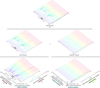Fig. 4 Illustration of the direct model for high-contrast long-slit spectroscopy given in Eq. (10). The data are modeled as the sum of two components: a stellar component and a companion component. Extracting the SED of the companion also requires the estimation of the on-axis PSF and the SED of the host star. The label “available via calibration” denotes components that may be self-calibrated by EXOSPECO directly from the science data (see Sect. 3.5 for details).

3.3 Objective function and regularization

After proper calibration of the detector, raw images are pre-processed to compensate for bias and gain non-uniformity and to identify defective pixels (i.e., pixels with a non-linear response). This pre-processing produces the long-slit spectroscopy data d ∈ ℝ^N considered here and modeled by m(x, y, z, v) in Eq. (15). Due to photon and detector noises as well as modeling inaccuracies, some discrepancies are expected between the data, d, and our model m(x, y, z, v). Due to the observed flux level, there are enough photons detected per pixel for the data, d, to approximately follow a Gaussian distribution of mean the model m(x, y, z, v) and of precision matrix⁷, W. Since we directly considered the data without any pixel interpolation (i.e., no image warping to align the dispersed speckles and no attempt to fix defective pixels), no correlations are introduced in the data and the pixels can be considered as mutually independent. The precision matrix is thus diagonal, W = diag(w) where w ∈ ℝ^N collects the diagonal entries of W and is given by: $$w_n\{\begin{array}{ll}0\hfill & \text{if\hspace{0.17em}}n\text{th\hspace{0.17em}pixel\hspace{0.17em}is\hspace{0.17em}invalid,}\hfill \\ 1/\text{Var}\left(d_n\right)\hfill & otherwise.\hfill \end{array}$$(16)

where Var(d_n) can be estimated by different pre-processing methods (Mugnier et al. 2004; Berdeu et al. 2020). We consider pixels to be invalid when the model is shown to be incorrect; this includes defective pixels, pixels that are overly impacted by the coronagraphic mask, and pixels located outside of the field of view (see Fig. 6). We assume that the estimation of the variances and the identification of defective pixels are part of the pre-processing stage. The definition of the precision matrix in Eq. (16) amounts to assuming that the variance of invalid pixels is infinite. In other words, this expresses that the values of invalid pixels should not be considered at all. Given the large number of unknowns, the estimation of the stellar and companion components x, y, and z cannot be performed solely by fitting the data: regularity constraints are necessary to prevent noise amplification and cope with missing data (Titterington 1985). We consider regularized estimators obtained by minimizing the following criterion: $$𝒞\left(x,y,z,v,\mu \right)=\left|\right|d-m\left(x,y,z,v\right)|{|}_W^2+{ℛ}_{xyz}\left(x,y,z,\mu \right),$$(17)

where the first term is a statistical distance between the model and the data (the co-log-likelihood) while ℛ_{x y z}(x, y, z, µ) is a regularization term parameterized by the vector µ of so-called hyper-parameters. In the above equation, ${\Vert u\Vert }_W^2=u^{\top }$ Wu denotes the squared Mahalanobis (1936) norm. Our estimators $\widehat{x}$, $\widehat{y}$, $\widehat{z}$, and $\widehat{v}$ of the parameters of interest are the ones that jointly minimize the criterion in Eq. (17): $$\begin{array}{lll}\left(\widehat{x}\left(\mu \right),\widehat{y}\left(\mu \right),\widehat{z}\left(\mu \right),\widehat{v}\left(\mu \right)\right)\hfill & =\hfill & \underset{\begin{array}{c}x\ge 0,y\ge 0,\\ z\ge 0,v\in \text{Ω}\end{array}}{\arg \min }𝒞\left(x,y,z,v,\mu \right).\hfill \end{array}$$(18)

These estimators depend on the hyper-parameters µ, as made explicit by the notation. As the parameters x, y, and z represent nonnegative quantities, their estimators are improved by enforcing nonnegativity as indicated by the inequality constraints in Eq. (18) such as x ≥ 0, which hold element-wise. The calibration parameters v = (v_⋆, v_⊕) are constrained to belong to a set Ω = Ω_⋆ × Ω_⊕ where Ω_⋆ and Ω_⊕ are the respective feasible sets for the stellar and companion calibration parameters defined based on physical considerations.

The SEDs and the on-axis PSF at the reference wavelength being mutually independent, the regularization function can be decomposed as: $${ℛ}_{xyz}\left(x,y,z,\mu \right)={\mu }_x{ℛ}_x\left(x\right)+{\mu }_y{ℛ}_y\left(y\right)+{\mu }_z{ℛ}_z\left(z\right).$$(19)

The complete set of hyper-parameters is then: $$\mu =\left({\mu }_x,{\mu }_y,{\mu }_z\right),$$(20)

where µ_x > 0, µ_y > 0, and µ_z > 0 tune the weights of the different regularization terms.

There are many regularizations that are suitable for our problem. Regularization terms should enforce some kind of continuity or smoothness of the sought uni-dimensional distributions. In the following (and for the sake of simplicity), we consider simple smoothness regularizations imposed by the quadratic penalty (Tikhonov & Arsenin 1977): $$ℛ\left(u\right)={\displaystyle {\sum }_{j=1}^{N_u-1}\underset{{\left(Du\right)}_j}{\underbrace{{\left(u_{j+1}-u_j\right)}^2}}={\Vert Du\Vert }_2^2,}$$(21)

with N_u the size of u = x, y, or z, and $D\in {ℝ}^{(N_u-1)\times N_u}$ a finite difference operator.

3.4 Alternating the minimization strategy

The joint minimization of the criterion defined in Eq. (17) requires us to cope with a highly non-linear function whose conditioning may be very bad and which depends on the scaling of the parameters. We propose to solve the problem by an alternated minimization strategy, that is, estimating each set of parameters given the others. Such a strategy consists in sequentially solving the following sub-problems: $$\begin{array}{l}\widehat{x}\left(y,r_{★},v_{★},{\mu }_x\right)=\underset{x\ge 0}{\arg \min }𝒞\left(x,y,z,v,\mu \right)\hfill \\ =\underset{x\ge 0}{\arg \min }\left\{{\Vert A_{★}x-r_{★}\Vert }_W^2+{\mu }_x{ℛ}_x\left(x\right)\right\},\hfill \end{array}$$(22a) $$\begin{array}{l}\widehat{y}\left(y,r_{★},v_{★},{\mu }_y\right)=\underset{y\ge 0}{\arg \min }𝒞\left(x,y,z,v,\mu \right)\hfill \\ =\underset{y\ge 0}{\arg \min }\left\{{\Vert B_{★}y-r_{★}\Vert }_W^2+{\mu }_y{ℛ}_y\left(y\right)\right\},\hfill \end{array}$$(22b) $$\begin{array}{l}{\widehat{v}}_{★}\left(x,y,r_{★}\right)=\underset{v_{★}\in {\text{Ω}}_{★}}{\arg \min }C\left(x,y,z,v,\mu \right)\hfill \\ =\underset{v_{★}\in {\text{Ω}}_{★}}{\arg \min }{\Vert m_{★}\left(x,y,v_{★}\right)-r_{★}\Vert }_W^2,\hfill \end{array}$$(22c) $$\begin{array}{l}{\widehat{z}}_{★}\left(r_{\oplus },v_{\oplus },{\mu }_z\right)=\underset{z\ge 0}{\arg \min }𝒞\left(x,y,z,v,\mu \right)\hfill \\ =\underset{z\ge 0}{\arg \min }\left\{{\Vert A_{\oplus }z-r_{\oplus }\Vert }_W^2+{\mu }_zℛ\left(z\right)\right\},\hfill \end{array}$$(22d) $$\begin{array}{l}{\widehat{v}}_{\oplus }\left(z,r_{\oplus }\right)=\underset{v_{\oplus }\in {\text{Ω}}_{\oplus }}{\arg \min }C\left(x,y,z,v,\mu \right)\hfill \\ =\underset{v_{\oplus }\in {\text{Ω}}_{\oplus }}{\arg \min }{\Vert m_{\oplus }\left(z,v_{\oplus }\right)-r_{\oplus }\Vert }_W^2,\hfill \end{array}$$(22e)

with: $$\forall x,A_{★}x=\gamma \odot \left(H_{★}\left(v\right)y\right)\odot \left(F_{★}x\right),$$(23a) $$\forall y,B_{★}y=\gamma \odot \left(F_{★}x\right)\odot \left(H_{★}\left(v\right)y\right),$$(23b) $$\forall z,A_{\oplus }z=\gamma \odot \left(h_{\oplus }\left(v\right)\right)\odot \left(F_{\oplus }z\right),$$(23c) $$r_{★}=d-m_{\oplus }\left(z,v_{\oplus }\right),$$(23d) $$r_{\oplus }=d-m_{★}\left(x,y,v_{★}\right),$$(23e) $$m_{★}\left(x,y,v_{★}\right)=\gamma \odot \left(H_{★}\left(v\right)y\right)\odot \left(F_{★}x\right)=A_{★}x=B_{★}y,$$(23f) $$m_{\oplus }\left(z,v_{\oplus }\right)=\gamma \odot h_{\oplus }\left(v\right)\odot \left(F_{\oplus }z\right)=A_{\oplus }z.$$(23g)

We enforced positivity constraints for the variables x, y, and z, while Ω_⋆ and Ω_⊕ (respectively) denote the feasible set of parameters v_⋆ and v_⊕. We note that m_⋆(x, y, v_⋆) and m_⊕(z, v_⊕) defined in Eqs. (23f) and (23g) are the respective contributions of the star and companion.

When the convex regularization defined in (21) is chosen and $A_{★}^{\text{T}}W{A}_{★}$, $B_{★}^{\text{T}}W{B}_{★}$, and $A_{\oplus }^{\text{T}}W{A}_{\oplus }$ are invertible, each of the problems (22a), (22b), and (22d) is strictly convex and thus has a unique solution that can be found by using existing algorithms⁸. This is another advantage of the alternated strategy. Since the original minimization problem (18) is not jointly convex with respect to all unknowns, only a local minimum is reached by the alternating minimization scheme, however.

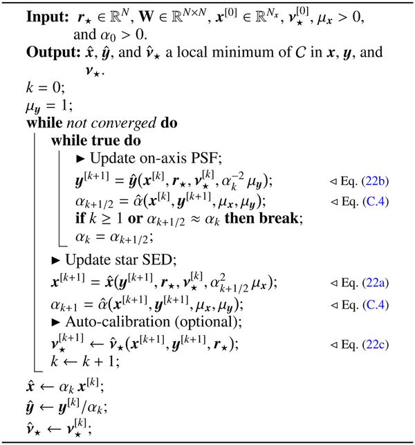
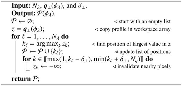
We solve for the two stellar components x and y following the alternated method proposed by Thé et al. (2020) to exploit the scaling indetermination of this problem (see Appendix C for details). This method is implemented by Algorithm 1 and takes as inputs the residuals r_⋆ = d – m_⊕(z, v_⊕) (i.e., the data without the contribution of the companion), the precision matrix, W, initial calibration parameters, $v_{★}^{[0]}$, the hyper-parameters, µ_x > 0 (hyper-parameter µ_y is set to the arbitrary value 1 in Algorithm 1), initial estimates, x^[0], of the stellar SED, and initial estimate, α₀ > 0, of the scaling parameter. We offer some remarks on Algorithm 1 below.

First, the initial stellar SED x^[0] must be such that ℛ_x(x^[0]) > 0 to be able to apply formula (C.4) to compute the optimal scaling factor (i.e., a non-flat SED). The initial stellar SED can be provided by calibration data (see Appendix B); otherwise, it can be computed from the science data, d, by the following weighted mean: $$\forall j\in 〚1,N_x〛:x_{★,j}^{\left[0\right]}=\frac{{\displaystyle {\sum }_{n\in {\chi }_j}{w}_n{d}_n}}{{\displaystyle {\sum }_{n\in {\chi }_j}}{w}_n},$$(24)

with w_n = W_n,n the nth diagonal term of the precision matrix and: $${\chi }_j=\left\{n\in 〚1,N〛|\left|{\lambda }_{★,j}^{\text{grd}}-{\lambda }_n\right|=\underset{j^{\prime }\in 〚1,N_x〛}{\min }\left|{\lambda }_{★,j^{\prime }}^{\text{grd}}-{\lambda }_n\right|\right\}$$(25)

the set of pixels whose nearest wavelength in the model grid is the jth one. Since Algorithm 1 scales the final components x^[k] and y^[k] by the corresponding optimal scaling factor, α₀ = 1 is a natural choice for the initial scaling factor in subsequent calls to Algorithm 1 (to refine the solution or after having improved the other parameters).

Second, the inner loop of Algorithm 1 avoids sensitivity to the initial scaling of the parameters (Thé et al. 2020). Then, the convergence criterion of Algorithm 1 is left unspecified. In our implementation, we chose to stop the algorithm when the relative change, in norm, between two consecutive iterates is smaller than a parameter ϵ (= 10⁻³).

Although they represent very different physical quantities, the problem is quite symmetric in variables x and y. Thus a variant of Algorithm 1 can be easily implemented to start with an initial estimate y^[0] of the stellar on-axis PSF at the reference wavelength instead of an initial estimate x^[0] of the stellar SED. For the very first run, this variant of Algorithm 1 is started with the weighted average of the on-axis PSF defined by: $$\forall j\in 〚1,N_y〛:y_{★,j}^{\left[0\right]}=\frac{{\displaystyle {\sum }_{n\in y_j}{w}_n{d}_n}}{{\displaystyle {\sum }_{n\in y_j}{w}_n}},$$(26)

with: $$y_j=\left\{n\in 〚1,N〛|\left|{\rho }_{★,j}^{\text{grd}}-{\rho }_n\right|=\underset{j^{\prime }\in 〚1,N_y〛}{\min }\left|{\rho }_{★,j^{\prime }}^{\text{grd}}-{\rho }_n\right|\right\},$$(27)

the set of pixels whose nearest angular position in the model grid is the jth one.

Finally, when the SED z of the companion is not yet known, it is sufficient to refer to Algorithm 1 with the weights of the pixels that are the most impacted by the companion set to zero (we denote the corresponding precision matrix as W_⋆) to estimate the components x and y of the stellar leakages without introducing a significant bias due to the contribution of the companion.

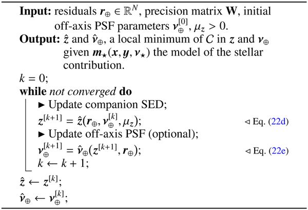
Algorithm 2 (FITCOMPANION) implements an alternated strategy to estimate the parameters z and v of the companion SED and its off-axis PSF at the reference wavelength. It takes as inputs the residuals r_⊕ = d – m_⋆ (x, y, v_⋆) (i.e., the data without the contribution of the star) and their respective weights W, the hyper-parameter µ_z > 0 and an initial estimate $v_{\oplus }^{\left[0\right]}\in {\text{Ω}}_{\oplus }$ of the parameters of the off-axis PSF at the reference wavelength.

These latter parameters can be given by the calibration described in Appendix B. Algorithm 2 also merits some remarks, which are given below.

First, the outputs of the algorithm only depend on the residual data r_⊕ defined in Eq. (23e) that need to be computed only once (on entry of the algorithm and not at each iterations).

Second, as in the case of Algorithm 1, various stopping criteria may be implemented to break the loop. Then, as with Algorithm 1, we can use the VMLM-B algorithm (Thiébaut 2002) to solve problem (22d) to estimate z under a non-negativity constraint.

In both algorithms, there are optional self-calibration steps performed by solving problem (22c) in Algorithm 1 (FITSTAR) and problem (22e) in Algorithm 2 (FITCOMPANION) to estimate the parameters of the on-axis and off-axis PSFs. These minimizations can be carried out by a derivative-free minimization algorithm. When there is a single calibration parameter, we use the Brent (2013) FMIN algorithm; if there are several parameters, we use one of Powell’s derivative-free methods NEWUOA or BOBYQA (Powell 2006, 2009) depending on the constraints defined by Ω.

3.5 The EXOSPECO algorithm

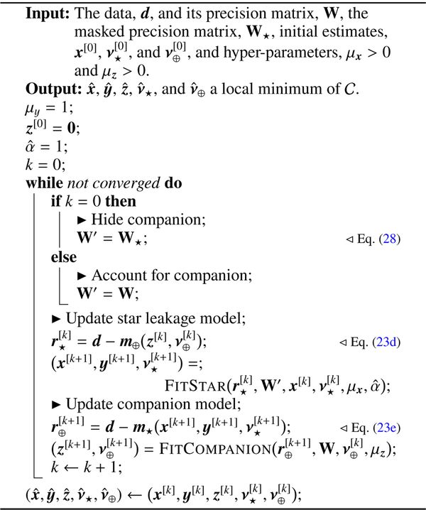
FITSTAR (Algorithm 1) and FITCOMPANION (Algorithm 2) are the building blocks of the EXOSPECO method given in Algorithm 3 for estimating all unknowns. A few additional remarks are given below.

First, for the first estimation of the stellar leakage parameters, it is beneficial to define a masked version, W_⋆, of the precision matrix of the data to avoid a significant bias of the first estimates due to the signal from the companion, which would slow down the convergence of Algorithm 3. The masked precision matrix is simply given by: $$W_{★}=\text{diag}\left(w_{★}\right)$$(28)

where the weights, w_⋆, are those of the precision matrix, W, of the data except that they are set to zero for the pixels that are the most impacted by the companion: $$\forall n\in 〚1,N〛:w_{★,n}=\{\begin{array}{ll}0\hfill & \text{if\hspace{0.17em}}{\gamma }_n\left|{\rho }_n-{\rho }_{\oplus }\right|\le \tau \hfill \\ w_n\hfill & \text{otherwise}\hfill \end{array}$$(29)

with τ > 0 the angular half-width at the reference wavelength of the impacted region. In practice, τ is taken to be 2–3 times ${\sigma }_{\oplus }^{\left[0\right]}$ the initial angular standard deviation of the off-axis PSF at the reference wavelength.

Then, the model of the stellar leakage only depends on either µ_x or µ_y, the other being arbitrarily chosen. For this reason, Algorithm 3 takes as inputs only two hyper-parameters, µ_x and µ_z, the remaining hyper-parameter being set to µ_y = 1.

After extracting the companion’s spectrum by the EXOSPECO Algorithm 3, it is possible to express it as a contrast relative to the host star that can be multiplied by a reference spectrum of the star to get rid of the atmospheric absorption (see Appendix B).

The auto-calibration steps in FITSTAR (Algorithm 1) and FITCoMPANIoN (Algorithm 2) are optional and consist in the resolution of problems (22c) and (22e). As these problems are non-convex, activating the auto-calibration at the beginning of the method can lead to a local minimum. To avoid such a behavior, it is possible to start the self-calibration of v_⋆ and v_⊕ only after a few iterations of EXOSPECO (Algorithm 3).

Controlling the number of inner iterations to solve each subproblem could be done by changing the value of the stopping parameter ϵ (cf. remark 3 in Sect. 3.4): the smaller ϵ the more inner iterations are needed and conversely. But this is expected to also impact the number of outer iterations. owing to the modest amount of time (2–3 min) taken by our implementation of EXOSPECO to solve the entire problem, we did not investigate whether the algorithm can be effectively accelerated by changing ϵ and keep the value ϵ = 10⁻³ suggested previously.

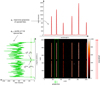Fig. 5 Calibration data for the SPHERE/IRDIS instrument and for the observations of HR 3549 on 2015/12/28. Central panel: calibration image. Left and top panels: projections of the calibration data along the 2nd spectral line (in green) and across all spectral lines (in red).

4 Calibration

The direct model in Eq. (15) assumes the physical coordinates (ρ_n, λ_n) of each pixel n of the detector are known. In this section, we offer a consistent approach to derive the spectro-angular dispersion laws of the instrument from calibration data.

4.1 Calibration data

Calibration data takes the form of an image (e.g., as shown in Fig. 5) obtained by illuminating the spectrograph slit with N_λ laser sources⁹. This produces N_λ mono-chromatic lines on the detector, each being interrupted by the coronagraphic mask. The calibration image d_cal is of size I × J and, for the calibration procedure, we denote it using n ~ (i, j) the one to one mapping between the pixel number, n, and its indices i ∈ ⟦1,I⟧ and j ∈ ⟦1, J⟧ along the first and second dimensions of the detector.

The calibration image shall have been pre-processed to compensate for bias and non-uniform response of the detector. Furthermore, we assume a given mask of valid pixels: $$w_{\text{msk},i,j}=\{\begin{array}{ll}1\hfill & \text{if\hspace{0.17em}the\hspace{0.17em}pixel\hspace{0.17em}}\left(i,j\right)\text{\hspace{0.17em}is\hspace{0.17em}valid,}\hfill \\ 0\hfill & \text{else}.\hfill \end{array}$$(30)

We considerapixelas being invalid ifits valuecannotfollow the assumed direct model given in Eq. (15). Invalid pixels include pixels outside the field of view, pixels under the coronagraphic mask or close to this mask, and defective pixels whose level does not linearly depend on the illumination. Figure 6 shows the mask of valid pixels for the HR 3549 data: the field of view and the coronagraphic mask are outlined by the two green trapezes, while the defective pixels are marked by green dots.

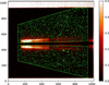Fig. 6 Valid pixel mask for the HR 3549 data observed on 2015-12-28 in MRS mode.

4.2 Dispersion laws

There are two dispersion laws to calibrate: A(i, j) for the wavelength and ϱ(i, j) for the separation angle along the slit. To determine the best approximation of these spectro-angular dispersion laws, we compared three models:

First, we have the “standard model” which assumes that the dispersion laws are uni-dimensional polynomials with spectral and angular directions aligned with the detector axes: $${\text{Λ}}_{\text{sta}}\left(i,j\right)={\displaystyle {\sum }_{p=0}^{P_{\lambda }}{a}_p}{j}^p,$$(31a) $${\varrho }_{\text{sta}}\left(i,j\right)={\displaystyle {\sum }_{p=0}^{P_{\rho }}{s}_p{i}^p},$$(31b)

with P_λ and P_ρ the degrees of the polynomials and {a_p}p∈⟦0,P_λ⟧ and {s_p}p∈⟦0,P_ρ⟧ their coefficients. For P_ρ = 1 and P_λ = 3–5, the “standard model” reproduces what is done in the software by Vigan et al. (2008) usually used to process SPHERE/LSS data.

Next, the model of medium complexity, also assuming 1D polynomials for the dispersion laws but accounting for misalignment angles ϕ_λ and ϕ_ρ ≈ ϕ_λ + 90°, respectively, between the spectral and angular directions and the detector axes: $${\text{Λ}}_{\text{med}}\left(i,j\right)={{\displaystyle {\sum }_{p=0}^{P_{\lambda }}{a}_p\left(i\sin {\varphi }_{\lambda }+j\cos {\varphi }_{\lambda }\right)}}^p,$$(32a) $${\varrho }_{\text{med}}\left(i,j\right)={{\displaystyle {\sum }_{p=0}^{P_{\rho }}{s}_p\left(i\sin {\varphi }_{\rho }+j\cos {\varphi }_{\rho }\right)}}^p.$$(32b)

We note that taking ϕ_λ = 0° and ϕ_ϱ = 90° yields the standard model.

Finally, a more complex model, which assumes 2D polynomials for the dispersion laws and, depending on the degree of these polynomials, can account for more complex image distortions than a simple rotation: $${\text{Λ}}_{\text{EXOSPECO}}\left(i,j\right)={\displaystyle {\sum }_{p_1=0}^{P_{\lambda }}{\displaystyle {\sum }_{p_2=0}^{P_{\lambda }-p_1}{a}_{p_1,p_2}{i}^{p_1}}}{j}^{p_2},$$(33a) $${\varrho }_{\text{EXOSPECO}}\left(i,j\right)={\displaystyle {\sum }_{p_1=0}^{P_{\rho }}{\displaystyle {\sum }_{p_2=0}^{P_{\rho }-p_1}{s}_{p_1,p_2}{i}^{p_1}}}{j}^{p_2}.$$(33b)

To summarize, the considered dispersion laws are polynomials of respective degree, P_λ and P_ρ. Their calibration amounts to fitting their coefficients a and s given the calibration image, d_cal, as explained in the next sub-sections.

4.3 Calibration of the spectral dispersion law Λ

To calibrate the spectral dispersion law Λ, we extract from the calibration image d_cal (see Fig. 5) the N_λ lists of pixel coordinates following the path of each spectral line on the detector and estimate the coefficients a by a least-squares fit: $$\widehat{a}=\underset{a}{\arg \min }{\displaystyle \sum _{\ell =1}^{N_{\lambda }}{{\displaystyle \sum _{\left(i,j\right)\in C_{\ell }\left({\varphi }_{\lambda }\right)}\left({\lambda }_{\ell }-\text{Λ}\left(i,j\right)\right)}}^2},$$(34)

where 𝒞_ℓ(ϕ_λ) denotes the list of, possibly fractional, pixel coordinates (i, j) along the ℓth spectral line on the detector. Since Λ(i, j) linearly depends on the coefficients a, then the solution â of the above problem has a closed-form expression (Lawson & Hanson 1974) that is easy to compute.

To extract the paths 𝒞_ℓ(ϕ_λ) of the spectral lines, we first compute a transverse projection q_⊥ (ϕ_λ) of the calibration image d_cal tuning the projection angle ϕ_λ, so as to maximize the peak values in the resulting projection. This transverse projection is plotted in red in the top panel of Fig. 5 and corresponds to ϕ_λ ≈ 0° for the considered calibration data. Equations (A.1) formally define how we carefully compute the projection avoiding invalid pixels. We then use the procedure described in Appendix A.2 to locate the position of the N_λ most significant peaks in the transverse projection q_⊥(ϕ_λ), which can be seen as a mean cross-section of the spectral lines. Finally, we use the method described in Appendix A.3 to extract the coordinates of the points defining the N_λ paths 𝒞_ℓ(ϕ_λ). These coordinates are given by the centers of gravity (again accounting for invalid pixels thanks to the mask) of the calibration data in small sliding rectangular windows along each spectral lines (see Appendix A.3 for details).

4.4 Calibration of the angular dispersion law ϱ

To calibrate the angular dispersion law ϱ, we extract from the calibration image d_cal (see Fig. 5), the positions of the edges of the coronagraphic mask for each of the N_λ spectral lines and estimate the coefficients s of the polynomial and the width Δρ of the mask by a least-squares fit: $$\begin{array}{l}\left({\widehat{\varphi }}_{\rho },\widehat{\text{Δ}}\rho ,\widehat{s}\right)=\underset{{\varphi }_{\rho },\text{Δ}\rho ,s}{\arg \min }\{{\displaystyle \sum _{\ell =1}^{N_{\lambda }}{\left(\varrho \left(i_{\ell }^{\text{down}},j_{\ell }^{\text{down}}\right)+\text{Δ}\rho /2\right)}^2}\hfill \\ +{\displaystyle \sum _{\ell =1}^{N_{\lambda }}{\left(\varrho \left(i_{\ell }^{\text{up}},j_{\ell }^{\text{up}}\right)-\text{Δ}\rho /2\right)}^2}\}\hfill \end{array}$$(35)

where ($i_{\ell }^{\text{down}}$, $j_{\ell }^{\text{down}}$) and ($i_{\ell }^{\text{up}}$, $j_{\ell }^{\text{up}}$) denote the coordinates of the edges of the coronagraphic mask respectively on the downhill and uphill sides along the profile of the ℓth spectral line. To solve this problem, we exploit that the criterion is quadratic in the unknowns s and Δρ, which thus have a closed-form solution (Lawson & Hanson 1974) that depends on ϕ_ρ. Replacing this closed-form solution in the criterion yields an uni-variate objective function that only depends on ϕ_ρ and which we minimize by Brent (2013) FMIN method starting at ϕ_ρ = ϕ_λ + 90°.

As explained in Appendix A.4, the coordinates of the edges of the coronagraphic mask for the ℓth spectral line are obtained from the longitudinal profile q_//ℓ(ϕ_λ) of the line which is the weighted projection, in a direction perpendicular to the transversal projection q_⊥(ϕ_λ), of the calibration data in a window encompassing the line. The longitudinal profile q _//ℓ(ϕ_λ) for the second (ℓ = 2) line is plotted in green in the left panel of Fig. 5 and the corresponding window is outlined in green in the central panel of Fig. 5.

4.5 Comparison of the calibration models

To compare the calibration models considered in Sect. 4.2, we applied EXOSPECO (Algorithm 3) on a scientific dataset of the star HR 3549 observed in MRS mode of SPHERE/IRDIS on 2015/12/28. Figure 7 shows the residuals r = d – m, that is the difference between the data and their model, computed for the different spectro-angular dispersion laws. This figure shows that the root mean square (rms) of the residuals are significantly reduced when using more flexible calibration models than the standard one. The improvement brought by the medium complexity model compared to the standard model proves that accounting for a slight angular misalignment between the spatial and spectral directions and the detector axes is important. Compared to the medium model, the complex model is able to account other image distortions than a simple rotation and thus achieves a better suppression of the stellar leakages. These results motivate the choice of the complex dispersion model in EXOSPECO to reduce the rms level of the residual stellar leakages by a factor of ~2 compared to the standard model and should therefore result in a better extraction of the companion contribution. We recall that the simple standard calibration model is similar to what is usually used for these data in other studies.

5 Validation and tuning of the method

To fully validate the method, we propose a study of the method on both real data and data where a synthetic companion was injected. This study allows us to both evaluate the modeling of the stellar leakages (and, thus, its subtraction in the residuals) and the extraction of the companion via a comparison with a ground truth spectrum. This study is described below.

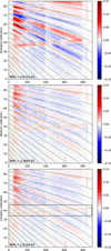Fig. 7 Residuals between the HR 3549 scientific data and the model of the stellar leakages, assuming a standard (top figure), medium (center), and complex (bottom) calibration models. The rms values of the residuals are given for each model. The iso-levels of ρ / λ which are approximately followed by the dispersed stellar speckles are plotted as green dashed lines. The position of the companion at the different wavelengths (i.e., at ρ = ρ⊕) is plotted as an orange dashed line.

5.1 Reduction of the self-subtraction

One of the main features of EXOSPECO is that it jointly estimates the contributions of the star and of the companion whose parameters are iteratively refined until convergence. Figure 8 shows the residuals close to the companion (in the region outlined by the black rectangle in the bottom of Fig. 7) with the complex model of the spatial and spectral dispersion laws in two cases: after the first outer iteration of EXOSPECO and after convergence of the algorithm. In the first outer iteration of EXOSPECO, the model of the stellar leakages is estimated by masking the region most impacted by the companion, as in Eq. (28), similarly to what is done by conventional methods. In all other outer iterations of EXOSPECO, the contribution of the other component is taken into account when fitting a given component (star or companion). As shown by the bottom panel of Fig. 8, there is a noticeable bias in the estimated companion’s SED after the first outer iteration. This so-called “self-subtraction bias” is mostly avoided by adopting the proposed alternating strategy.

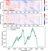Fig. 8 Residuals between the HR 3549 scientific data and the model of the stellar leakages near the companion (defined by the black rectangle in the bottom of Fig. 7) and for the complex model of the spatial and spectral dispersion laws after one iteration (top) and after convergence (middle) of EXOSPECO. The rms of the residuals in this region are significantly reduced after convergence. The orange dashed line indicates the position of the companion at the different wavelengths. The SEDs of the companion (including atmospheric absorption) extracted from these residuals are plotted in the bottom-most panel.

5.2 Tuning of the regularization parameters

As described in Appendix C, the fact that the model of the star leakages is bi-linear makes it possible to tune the regularization of this component by a single hyper-parameter, that is, the other hyper-parameter being held fixed. Thanks to this, the solution found by EXOSPECO only depends on two hyper-parameters: one for the star, say, µ_x (while µ_y = 1 is imposed) and one for the companion, µ_z. In this section, we highlight the incidence on the companion SED extracted by EXOSPECO of these remaining hyper-parameters using the same scientific data set as in Sect. 4.5.

Figure 9 shows the SEDs of the companion estimated by EXOSPECO for different values of the star regularization hyper-parameters (µ_y = 1 and µ_x = 10⁻³, 10, and 10⁵). For such a broad range of values, the differences between the extracted companion SEDs are smaller than 1%. The stellar regularization hyper-parameters have thus a limited impact on the resulting companion SED. The tuning of µ_x can thus reasonably be done by visual inspection.

On the contrary, as Fig. 10 shows, the hyper-parameter µ_z has a strong impact on the resulting companion SED. This is expected as µ_z directly tunes the strength of the smoothness constraint for the companion SED z. This hyper-parameter has thus to be carefully chosen to find the best compromise between a solution that is too smooth (e.g., for µ_z = 10⁷ in Fig. 10) or too noisy (e.g., for µ_z = 10² in Fig. 10). It is worth noticing that the correct value of µ_z strongly depends on the considered data, so µ_z = 10⁵, which seems to be a good choice for the HR 3549 data (see Fig. 10), should not be considered as a universal value.

Many methods have been proposed to automatically tune the hyper-parameter(s) of an inverse problem: a generalized cross-validation (CGV; Golub et al. 1979), Stein’s unbiased risk estimate (SURE; Stein 1981), hierarchical Bayesian method (Molina 1994), or the L-curve (Hansen & O’Leary 1993) to mention a few that could potentially be used with our extraction algorithm. Implementing and testing these methods for EXOSPECO is beyond the scope of this paper. However, since the companion SED found by EXOSPECO does not strongly depend on the tuning of the stellar regularization, our method is mostly driven by a single hyper-parameter, µ_z, the level of the regularization for the companion SED. This greatly reduces the complexity of tuning the EXOSPECO algorithm.

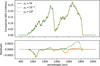Fig. 9 Top: profiles of the companion SED z, for different levels of the stellar hyper-parameter µx and with µy = 1 and µz = 105. Bottom: differences between the profile for µx = 10 and the profiles for µx = 10−3 (dashed orange) and µx = 105 (dotted green).

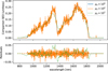Fig. 10 Profiles of the companion SED z for different levels of the companion regularization (µz = 102 in dashed orange, µz = 105 in blue, and µz = 107 in dotted green) in the top panel. Differences between the profile for µz = 105 and the profiles for µz = 102 (dashed orange) and µz = 107 (dotted green) at the bottom. For all these results, the stellar hyper-parameters are µx = 10 and µy = 1.

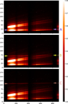Fig. 11 Scientific data of HIP 65426 with a synthetic companion whose contrast is χ = 2 × 10−4 relative to the star and injected at angular separations ρ⊕ − ρ★ = 273 mas (A), 890 mas (B), and 1353 mas (C) indicated by the arrows.

5.3 Extraction of simulated spectrum in real data

To validate the EXOSPECO method, we injected the contribution of a synthetic companion in existing SPHERE/IRDIS MRS data d of the star HIP 65426 observed on 2019-05-20. Although HIP 65426 star hosts a planet (Chauvin et al. 2017; Carter et al. 2023), the frame was selected for the de-rotation angles hiding the planet outside the slit. The off-axis PSF h_⊕ of the synthetic companion follows the model in Eqs. (13) and (14c) with σ_⊕ set to match the diffraction limit of the telescope at the reference wavelength λ^ref and with different angular positions ρ_⊕ on the side of the coronagraphic mask where no companion was detected. The “ground truth” SED of the synthetic companion is z_gt = χ x_flux, where χ > 0 is the mean contrast of the companion relative to the star (without a coronagraph) and x_flux is the SED of the star HIP 65426 calibrated as explained in Appendix B. We used a constant contrast for all wavelengths (i.e., the SED of the star and of the companion are the same, up to the contrast χ). Figure 11 shows examples of generated data with a synthetic companion whose contrast with respect to the star is χ = 2 × 10⁻⁴ and which is injected at different angular separations, ρ_⊕ − − ρ_★.

To assess the quality of the extracted companion’s SED $\widehat{z}$, we compute the following relative error: $$q=\frac{{\displaystyle {\sum }_{j=1}^{N_z}\left|z_{\text{gt},j}-{\widehat{z}}_j\right|}}{{\displaystyle {\sum }_{j=1}^{N_z}\left|z_{\text{gt},j}\right|}}.$$(36)

In the following tests, the value of µ_z, the regularization level of the companion’s SED, has been tuned so as to minimize the relative error q. Figure 12 plots the relative error q for synthetic companions injected at angular separations ρ_⊕ − ρ_★ ranging from 200 mas to 1850 mas and with contrasts χ = 3 × 10⁻⁵, 2 × 10⁻⁴, and 2 × 10⁻³. Clearly, the quality of the recovered SEDs degrades as the companion gets closer to the mask. This is expected because, when getting closer to the mask, not only are the stellar leakages brighter (thus causing more photon noise in the residuals) but the approximation by the assumed off-axis PSF model also worsens. For angular separations larger than ~600 mas and for all considered contrasts, the quality of the recovered SEDs improves as the separation increases until a plateau is reached at ρ_⊕ − ρ_★ ~ 1400 mas, where the dominant source of nuisance is the readout noise.

Figure 13 shows examples of recovered companion SEDs $\widehat{z}$ at angular separations ρ_⊕ − ρ_★ = 273 mas (A), 890 mas (B), and 1353 mas (C) for the same contrasts χ as in Fig. 12. Figure 13 confirms that the relative error q does reflect the ability of our method to reliably recover the companion SED. When q ≤ 0.1 (the green curves for angular separations B and C and the orange curve for angular separation C), all the features of the SED are correctly recovered. For q ~ 0.2 (the green curve for case A, the orange curve for case B, and the blue curve for case C), the global shape of the SED is restored but with small spectral features smoothed out and some photometric biases. These cases prove that it is possible to extract a coarse but still exploitable SED for bright companions quite close to the mask, typically χ > 10⁻³ for ρ_⊕ − ρ_★ ~ 250 mas, from a single MRS exposure.

The angular separation must be larger for fainter companions; for example, ρ_⊕ − ρ_★ ≥ 1200 mas for χ ~ 2 × 10⁻⁵. The photometric biases in the most difficult cases (the green curve in case A, the orange one in case B, and the blue one in case C) clearly indicates that the removal of the modeled stellar contribution leaves non-negligible residuals compared to the companion. A possible improvement could be to use a more complex model of the on-axis PSF and consider more than one mode in the series expansion of Eq. (3).

To summarize the performances of the current version of EXOSPECO for a single data frame of the HIP 65426 observations, Fig. 14 plots the minimal contrast needed to achieve a given relative error q as a function of the angular separation. The figure shows that by tolerating a relative error as high as q = 0.3, a companion with a contrast up to χ ~ 2 × 10⁻⁵ can be characterized. In our conclusions, we explain how to extend EXOSPECO to jointly process several data frames in order to increase the sensitivity of the algorithm.

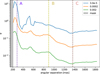Fig. 12 Relative error q defined in Eq. (36) for synthetic companions injected in the scientific data of HIP 65426 (with the same spectra as the host star) as a function of the angular separation, ρ⊕ − ρ★, and for contrasts of χ = 3 × 10−5 (blue), 2 × 10−4 (orange), and 2 × 10−2 (green). The grayed area represents the region invalidated by the coronagraphic mask. The angular separations of the three cases presented in Fig. 11 are highlighted by the dashed lines labeled A, B, and C.

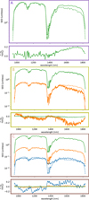Fig. 13 Examples of recovered companion SEDs $\widehat{z}$ in the same conditions as in Figs. 11 and 12 for synthetic companions injected at angular separations ρ⊕ − ρ★ = 273 mas (A), 890 mas (B), and 1353 mas (C) with contrasts of χ = 3 × 10−5 (blue curves), 2 × 10−4 (orange curves), and 2 × 10−2 (green curves). The ground truth SED zgt is plotted in dashed lines. The normalized residuals are plotted below each panel.

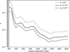Fig. 14 Minimal contrast χ required to achieve a given relative error q as a function of the angular separation. The conditions are the same as in Figs. 11 and 12.

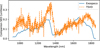Fig. 15 Comparison of the SEDs extracted from the HR 3549 data by EXOSPECO and by a standard TSVD method. See text for details.

5.4 Comparison with TSVD extraction

We compared EXOSPECO to a standard approach based on the TSVD method described in Sect. 2.2 to remove the stellar leakages. Figure 15 shows the companion SED extracted from the HR 3549 data by EXOSPECO and by the TSVD approach. For the latter method, the SED of the companion was extracted by local averaging in a 7 pixel height sliding window along the companion signal in the residual image given by Eq. (7) and shown in Fig. 3. In both cases, the same complex calibration model of the spectral and angular dispersion laws described in Appendix A has been used. In spite of this identical calibration, the two extracted SEDs are notably different. Thanks to the optimal extraction in the maximum likelihood sense and to the spectral regularization, the SED extracted by EXOSPECO is smoother and less noisy. At a coarser resolution, the two SEDs display quite different spectral features. However, without a known ground truth, the two SEDs cannot be ranked. For this reason, we also compared the results given by the two methods on a synthetic injection done as described in Sect. 5.3. Figure 16 clearly demonstrates that not only does EXOSPECO produce less noisy results, but that they also offer a better reflection of reality.

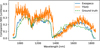Fig. 16 Comparison of the SEDs extracted from semi-synthetic data by EXOSPECO and by a standard TSVD method. The angular separation and the contrast of the injected companion are respectively ρ⊕ − ρ★ = 785 mas and χ = 2 × 10−4. The green dashed curve represents the ground truth injected spectrum which is that of HIP 65426 multiplied by χ.

6 Conclusion

In this paper, we present a novel algorithm, EXOSPECO, to extract the spectrum of a companion from high-contrast long-slit spectroscopic data. The most challenging part of such a processing is to disentangle the signal of interest from the stellar leakages since they are much brighter. Compared to existing methods, our algorithm avoids any transform of the data, whether it is to align the speckles of the stellar leakages at all wavelengths or to fix defective pixels. EXOSPECO has also the advantage of jointly extracting the parameters describing the stellar leakages (the star spectrum and the on-axis PSF), the companion spectrum, the off-axis PSF, and, optionally, some calibration parameters. By using non-uniform statistical weights for the data pixels, our approach is optimal in the maximum likelihood sense, namely, it takes into account all available measurements and consistently treats defective pixels as missing data. The joint optimization problem having no closed-form solution, we proposed an alternating minimization strategy which has proven to be effective. In spite of the numerous parameters coming into play in the algorithm, the outputs of the method are, in practice, mostly driven by a single hyper-parameter that tunes the level of regularization of the companion SED.

Although it is not directly part of the spectrum extraction algorithm, we have shown that careful calibration of the instrument is critical to get rid of the contamination by the stellar leakages. For that purpose, we described a refined calibration method of the spectral and spatial dispersion laws from available calibration data. In particular, SPHERE/LSS data present a misalignment of the principal directions of dispersion with the detector axes as well as a geometrical shear. If they are not accounted for, we show that these distortions have a detrimental impact on the result of the processing, whether it is by EXOSPECO or by the current state-of-the-art method. A few remaining calibration parameters that may depend on the observing conditions, such as the off-axis PSF size and the precise locations of the star and of the companion along the slit, can be optionally adjusted by a self-calibration procedure built into EXOSPECO. Thanks to this calibration step, our method significantly reduces the “self-subtracting” bias by better disentangling the stellar leakages component from the companion component. A Julia (Bezanson et al. 2017) implementation of EXOSPECO is freely available¹⁰, with an implementation of the calibration method described in Sect. 4 and Appendix A¹¹.

Based on tests carried on empirical long-slit spectroscopic data and on injections of a synthetic companion signal in these data, we demonstrated that the proposed approach effectively avoids the self-subtraction bias, even very close to the coronagraphic mask. We provided curves to predict the minimal contrast required to achieve a given quality of extraction of the companion SED. Reliable extraction of a companion SED can be achieved from a single data frame at contrasts as low as a few 10⁻⁵. The proposed method could boost the characterization of known (faint) exoplanets at a spectral resolution substantially higher than currently possible with SPHERE IFS (R ~ 35 – 50) and for contrasts much better than achievable with IRDIS MRS using state of the art methods. By capturing more the stellar contamination efficiently, the method we propose does not require independent and thus imperfect calibration of the speckles by rotating the slit to hide the planet signal. This will typically gain at least 50% in telescope time while reaching (and even surpassing) the same contrast limit. This new method also paves the way to combining polarimetry and spectroscopic measurements with IRDIS LSS mode (R. Holstein, priv. comm.).

As it is based on an inverse problems framework, EXOSPECO is very flexible and can be adapted to various kinds of data (such as data sequences or data from other instruments). An example of such an extension of EXOSPECO is the joint processing of multiple frames that can be done as follows. Assuming T LSS exposures d₁ to d_T of the same object are collected during a night, they can be combined into a single criterion that extends Eq. (17): $$\begin{array}{l}\text{𝒞}\left(x,y_1,y_2,\dots y_T,z,v,\mu \right)\hfill \\ ={\displaystyle \sum _{t=1}^T{\Vert d_t-m\left(x,y_t,z,v\right)\Vert }_{W_t}^2+{\mu }_x{\text{ℛ}}_x\left(x_t\right)}\hfill \\ +{\mu }_y{\displaystyle \sum _{t=1}^T{\text{ℛ}}_y\left(y_t\right)+{\mu }_z{\text{ℛ}}_z\left(z\right)},\hfill \end{array}$$(37)

where the statistical independence of noise between frames is considered (a natural assumption). This criterion can be minimized in x, y₁, …, y_T, z, and v following the same alternating method as described in Sect. 3.4, only with more steps in order to estimate the on-axis PSF at each of the T frames. Such a joint processing has the potential to improve the estimation of companion SEDs and push further the achievable contrast limit.

Finally, to better disentangle the stellar leakages from the companion spectrum, the model of the on-axis PSF could be improved by taking into account more spatial modes of the series expansion in Eq. (3). Indeed, as demonstrated in Devaney & Thiébaut (2017), accounting for more such modes significantly improves the modeling of the stellar leakages, especially near the coronagraphic mask. Such an improvement would not call into question the founding principles of EXOSPECO, but it would require an optimization strategy to be adopted.

Acknowledgements

This work was supported by the Action Spécifique Haute Résolution Angulaire (ASHRA) of CNRS/INSU co-funded by CNES. SPHERE is an instrument designed and built by a consortium consisting of IPAG (Grenoble, France), MPIA (Heidelberg, Germany), LAM (Marseille, France), LESIA (Paris, France), Laboratoire Lagrange (Nice, France), INAF – Osservatorio di Padova (Italy), Observatoire de Genève (Switzerland), ETH Zürich (Switzerland), NOVA (Netherlands), ONERA (France) and ASTRON (Netherlands) in collaboration with ESO. SPHERE was funded by ESO, with additional contributions from CNRS (France), MPIA (Germany), INAF (Italy), FINES (Switzerland) and NOVA (Netherlands). SPHERE also received funding from the European Commission Sixth and Seventh Framework Programmes as part of the Optical Infrared Coordination Network for Astronomy (OPTICON) under grant number RII3-Ct-2004-001566 for FP6 (2004–2008), grant number 226604 for FP7 (2009–2012) and grant number 312430 for FP7 (2013–2016).

Appendix A Calibration of the spectro-angular dispersion laws

This appendix provides some details about the methods used for the calibration of the spectro-angular laws described in Sect. 4 and some figures to support the results discussed in Sect. 4.5. The considered calibration data d_cal is the image in the central panel of Fig. 5.

A.1 Transverse projection

To locate the positions of the spectral lines, we compute a weighted transverse projection of the calibration image d_cal: $$q_{\perp k}\left({\varphi }_{\lambda }\right)=\frac{{\displaystyle \sum {}_{i,j}{\xi }_{\perp i,j,n}\left({\varphi }_{\lambda }\right)d_{\text{cal,}i,j}}}{{\displaystyle \sum {}_{i,j}{\xi }_{\perp i,j,n}\left({\varphi }_{\lambda }\right)}},$$(A.1a)

with weights given by: $${\xi }_{\perp i,j,k}\left({\varphi }_{\lambda }\right)=w_{\text{msk,}i,j}{\phi }_{\text{proj}}\left(i\sin {\varphi }_{\lambda }+j\cos {\varphi }_{\lambda }-k\right)$$(A.1b)

and for a projection angle, ϕ_λ, chosen to maximize the peak values of the resulting projection (plotted in red in the top panel of Fig. 5 for ϕ_λ ≈ 0°). In practice, we take φ_proj(t) = max(1 − |t|, 0), the linear B-spline, as the interpolating function for the projection. We note that thanks to the weighting by the mask of valid pixels w_msk defined in Eq. (30), invalid pixels have no incidence on the computed projection.

A.2 Detection of the spectral peaks

We use algorithm 4 with tolerance parameter δ_⊥ = 10 pixels to find the N_λ most significant peaks in the transverse projection $q_{\perp }\left({\varphi }_{\lambda }\right)\in {ℝ}^{N_q}$ computed according to Eq. (A.1).

A.3 Extraction of the paths of the spectral lines

Given the projection angle ϕ_λ and the list 𝒫(ϕ_λ) of the N_λ most significant peaks in the transverse projection, q_⊥(ϕ_λ), we build the ℓth spectral path 𝒞_ℓ as a list of points along the ℓth spectral line. The coordinates, ($i_{\ell ,m}^{\text{path}}$, $j_{\ell ,m}^{\text{path}}$), of the mth such point are given by computing the center of gravity of the calibration data in a small rectangular window, 𝒲_ℓ,m(ϕ_λ), sliding along the considered spectral lines: $$(i_{\ell ,m}^{\text{path}},j_{\ell ,m}^{\text{path}})=\frac{{\displaystyle \sum {}_{(i,j)\in }{𝒲}_{\ell .m}{}_{({\varphi }_{\lambda })}{w}_{\text{msk},i,j}}\times (i,j)}{{\displaystyle \sum {}_{(i,j)\in }{𝒲}_{\ell .m}{}_{({\varphi }_{\lambda })}{w}_{\text{msk},i,j}}},$$(A.2)

computed for all non-empty¹² sliding window 𝒲_ℓ,m of size ~ 1 pixel along the spectral line and 2 δ_⊥ + 1 pixels in the perpendicular direction: $${\mathcal{W}}_{\ell ,m}\left({\varphi }_{\lambda }\right)=\left\{\begin{array}{c}(i,j)\in 〚1,I〛\times 〚1,J〛\text{ such that }\\ \left|i\sin {\varphi }_{\lambda }+j\cos {\varphi }_{\lambda }-k_{\ell }\right|\le {\delta }_{\perp }+\frac{1}{2}\\ \text{ and }\left|i\cos {\varphi }_{\lambda }-j\sin {\varphi }_{\lambda }-m\right|\le \frac{1}{2}\end{array}\right\},$$(A.3)

where k_ℓ is the ℓth index in the list 𝒫(ϕ_λ) of the N_λ most significant peaks in the transverse projection q_⊥(ϕ_λ). Again, we note that thanks to the weighting by the mask of valid pixels, invalid pixels have no incidence on the computed coordinates. In practice, we use the same value for the half-width of the sliding windows and for the minimal separation between peaks in the transverse projection, that is δ_⊥ = 10 pixels for the considered calibration data.

A.4 Detection of the edges of the spectral bands

Given the projection angle, ϕ_λ, and the list, 𝒫(ϕ_λ), of the N_λ most significant peaks in the transverse projection q_⊥(ϕ_λ), we compute the longitudinal profile of each spectral line as the following weighted projection: $$q_{//\ell ,k}({\varphi }_{\lambda })=\frac{{\displaystyle \sum {}_{(i,j)\in {𝒟}_{\ell }({\varphi }_{\lambda })}{\xi }_{//i,j,k}({\varphi }_{\lambda })d_{\text{cal},i,j}}}{{\displaystyle \sum {}_{(i,j)\in {𝒟}_{\ell }({\varphi }_{\lambda })}{\xi }_{//i,j,k}({\varphi }_{\lambda })}},$$(A.4a)

with weights given by: $${\xi }_{//i,j,k}({\varphi }_{\lambda })=w_{\text{msk},i,j}{\phi }_{\text{proj}}(i\cos {\varphi }_{\lambda }-j\sin {\varphi }_{\lambda }-k),$$(A.4b)

and where k is the index along the projection and 𝒟_ℓ(ϕ_λ) is a narrow rectangular window (in green in the central panel of Fig. 5) to isolate the pixels of the calibration image, d_cal, impacted by the considered spectral line: $${𝒟}_{\ell }({\varphi }_{\lambda })=\left\{\begin{array}{c}(i,j)\in 〚1,I〛\times 〚1,J〛,\text{\hspace{0.17em}such\hspace{0.17em}that}\\ |i\sin {\varphi }_{\lambda }+j\cos {\varphi }_{\lambda }{k}_{\ell }|\le {\delta }_{\perp }+\frac{1}{2}\end{array}\right\}$$(A.5)

with, as before, δ_⊥ ≈ 10 pixels the half-width of the region.

Detecting the edges of the central hole due to the corona-graphic mask in the resulting profile (plotted in green in the left panel of Fig. 5) can be done by a quite simple procedure. Each value at index k of the profile is compared with the next one up to a threshold value τ. If q_//ℓ,k ⩿ τ ⩿ q_//ℓ,k+1 and q_//ℓ,k < q_//ℓ,k+1, then an ascending edge is detected. If q_//ℓ,k ⩾ τ ⩾ q_//ℓ,k+1 and q_//ℓ,k > q_//ℓ,k+1, it is a descending edge. From the four edges detected in the ℓth spectral line (indicated by the crosses in the left panel of Fig. 5), the second and third ones correspond to the coronagraphic mask. Retrieving these edges in 𝒞_ℓ(ϕ_λ) yields the coordinates ($i_{\ell }^{\text{down}}$, $j_{\ell }^{\text{down}}$) and ($i_{\ell }^{\text{up}}$, $j_{\ell }^{\text{up}}$) required in Sect. 4.4 for the calibration of the angular dispersion law.

A.5 Results on the calibration data

The results of the proposed calibration models are displayed in Fig. A.1, as blue lines for the spectral law and green lines for the spatial law. In practice, degrees P_λ = 5 and P_ρ = 1 (limited by the small number of points for ρ) were chosen. The three models described in Sect. 4.2 are tested, that is a standard model, one of a medium complexity and one more complex.

As can be seen on the different zooms shown in Fig. A.2, 2D polynomials are needed to explain local distortions. Choosing this model, we plot on Fig. A.3 some iso-wavelength (blue) and iso-angular distance (green) curves, on a zoom in of the HR3549 dataset. This figure highlights how well our proposed models for the dispersion laws are following the speckles, compared to the standard model. A strong shear effect due to the dispersive elements is visible and taken into account by our model. For all these models, we took polynomials of degrees P_λ = 5 and P_ρ = 1 for the spectral and spatial dispersion laws.

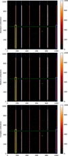Fig. A.1 Iso-wavelength curves at the wavelengths of the calibration sources (blue lines) and iso-angular distance of the center of the coron-agraphic mask of (green lines) presented on top of the calibration data, dcal. The upper panel presents the results for the simple model, the central panel shows the results for the medium model, while the bottom panel shows the results of using the complex model.

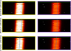Fig. A.2 Magnified images of the two regions outlined by the yellow and purple rectangles for the three models described in Sect. 4.2. To best see the differences between models, the magnifications are different in the two dimensions.

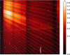Fig. A.3 Iso-wavelength and iso-angular distance superposed to the HR 3549 data observed on 2015-12-28 with IRDIS in MRS mode.

Appendix B Calibration of the contrast

In order to express the SED of the companion in terms of contrast with respect to the star, we use specific calibration data, d_flux, (shown in Fig. B.1, top panel) for which the star is placed in the spectrograph slit but shifted away from the coronagraphic mask and with a neutral density inserted in the optical path to avoid detector saturation. Applying FITCOMPANION (algorithm 2) to d_flux and dividing the resulting SED by the spectral transmission of the neutral filter yields the SED of the star x_flux (shown in Fig. B.1, bottom panel). The so derived parameters of the off-axis PSF can be later used in FITCOMPANION (algorithm 2) to extract the companion SED.

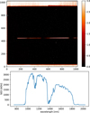Fig. B.1 Calibration of the SED of the star HIP 65426. Top: Calibration image dflux observed on 2019-05-20 with the MRS mode of SPHERE/IRDIS. Bottom: SED of the star extracted by FITSTAR (algorithm 2) and corrected from the density filter.

Appendix C Exploiting the scaling indetermination

The estimated components $\widehat{x}$, $\widehat{y}$, $\widehat{z}$, and $\widehat{v}$ of the direct model defined in Eq. (15) depend on hyper-parameters which include the regularization weights µ_x, µ_y, and µ_z. In this appendix, we show how to adapt the approach of Thé et al. (2020) to reduce the effective number of regularization parameters and also accelerate the minimization.

We first note that the regularizations considered for the stellar components are homogeneous functions of degree 2, namely, the following property holds: $${ℛ}_u(\alpha u)={\alpha }^2{ℛ}_u(u),$$(C.1)

whatever the component u = x or y considered and α ≥ 0.

The contribution of the star, the first right-hand side term in Eq. (15), is a bilinear function of the parameters x and y. As a consequence: $$m(\alpha x,y/\alpha ,z,v)=m(x,y,z,v)$$(C.2)

holds for any scaling factor α > 0.

Combining the properties in Eqs. (C.1) and (C.2) with the definition of the objective function in Eq. (17) and that of the regularization in Eq. (19), it can be seen that for any α > 0: $$\mathcal{C}\left(\alpha x,y/\alpha ,z,v,{\mu }_x,{\mu }_y,{\mu }_z\right)=C\left(x,y,z,v,{\alpha }^2{\mu }_x,{\alpha }^{-2}{\mu }_y,{\mu }_z\right).$$(C.3)

In other words, scaling the unknowns x and y without changing the model is equivalent to scaling their regularization weights.

Exploiting this, it is possible to compute an optimal scaling factor: $$\begin{array}{c}\widehat{\alpha }\left(x,y,{\mu }_x,{\mu }_y\right)=\underset{\alpha >0}{\arg \min }C\left(\alpha x,y/\alpha ,z,v,{\mu }_x,{\mu }_y,{\mu }_z\right)\\ =\underset{\alpha >0}{\arg \min }C\left(x,y,z,v,{\alpha }^2{\mu }_x,{\alpha }^{-2}{\mu }_y,{\mu }_z\right)\\ =\underset{\alpha >0}{\arg \min }\left\{{\alpha }^2{\mu }_x{ℛ}_x(x)+{\alpha }^{-2}{\mu }_y{ℛ}_y(y)\right\}\\ ={\left(\frac{{\mu }_y{ℛ}_y(y)}{{\mu }_x{ℛ}_x(x)}\right)}^{\frac{1}{4}}.\end{array}$$(C.4)

Plugging this expression in the definition of the criterion yields: $$\begin{array}{l}{C}^{+}\left(x,y,z,v,{\mu }_x,{\mu }_y,{\mu }_z\right)\hfill \\ =\underset{\alpha >0}{\min }C\left(\alpha x,y/\alpha ,z,v,{\mu }_x,{\mu }_y,{\mu }_z\right)\hfill \\ ={\Vert d-m\left(x,y,z,v\right)\Vert }_{\text{W}}^2+{\mu }_{x,y}{ℛ}_{x,y}\left(x,y\right)+{\mu }_z{ℛ}_z\left(z\right)\hfill \end{array}$$(C.5)

where: $${ℛ}_{x,y}(x,y)=\sqrt{{ℛ}_x(x){ℛ}_y(y),}$$(C.6)

and: $${\mu }_{x,y}=2\sqrt{{\mu }_x{\mu }_y.}$$(C.7)

This shows that the regularizations of the stellar components x and y are entangled and that the effect of these regularizations on the shape of these components is effectively controlled by a single hyper-parameter; here, this is µ_x,_y. As shown by Eq. (C.4), the ratio µ_x /µ_y of the hyper-parameters controls the scaling, not the shape, of x and y, one of the two can be fixed. This saves us the hassle of adjusting both parameters at the same time.

References

- Berdeu, A., Soulez, F., Denis, L., Langlois, M., & Thiébaut, É. 2020, A&A, 635, A90 [NASA ADS] [CrossRef] [EDP Sciences] [Google Scholar]
- Beuzit, J. L., Vigan, A., Mouillet, D., et al. 2019, A&A, 631, A155 [NASA ADS] [CrossRef] [EDP Sciences] [Google Scholar]
- Bezanson, J., Edelman, A., Karpinski, S., & Shah, V. B. 2017, SIAM Rev., 59, 65 [Google Scholar]
- Brent, R. 2013, Algorithms for Minimization Without Derivatives (Dover Publications) [Google Scholar]
- Carter, A. L., Hinkley, S., Kammerer, J., et al. 2023, ApJ, 951, L20 [NASA ADS] [CrossRef] [Google Scholar]
- Catmull, E., & Rom, R. 1974, in Computer Aided Geometric Design, eds. R. E. Barnhill, & R. F. Riesenfeld (Academic Press), 317 [CrossRef] [Google Scholar]
- Chauvin, G., Desidera, S., Lagrange, A.-M., et al. 2017, A&A, 605, A9 [Google Scholar]
- Dallant, J., Langlois, M., Thiébaut, É. M., & Flasseur, O. 2022, Proc. SPIE, 12185, 1218537 [NASA ADS] [Google Scholar]
- Devaney, N., & Thiébaut, É. 2017, MNRAS, 472, 3734 [NASA ADS] [CrossRef] [Google Scholar]
- Dohlen, K., Langlois, M., Saisse, M., et al. 2008, SPIE Conf. Ser., 7014, 70143L [Google Scholar]
- Eckart, C., & Young, G. 1936, Psychometrika, 1, 211 [CrossRef] [Google Scholar]
- Flasseur, O., Denis, L., Thiébaut, É., & Langlois, M. 2018, A&A, 618, A138 [NASA ADS] [CrossRef] [EDP Sciences] [Google Scholar]
- Flasseur, O., Denis, L., Thiébaut, É., & Langlois, M. 2020a, A&A, 637, A9 [NASA ADS] [CrossRef] [EDP Sciences] [Google Scholar]
- Flasseur, O., Denis, L., Thiébaut, É., & Langlois, M. 2020b, A&A, 634, A2 [Google Scholar]
- Golub, G. H., Heath, M., & Wahba, G. 1979, Technometrics, 21, 215 [Google Scholar]
- Hansen, P. C., & O’Leary, D. P. 1993, SIAM J. Sci. Comput., 14, 1487 [NASA ADS] [CrossRef] [Google Scholar]
- Jovanovic, N., Martinache, F., Guyon, O., et al. 2015, PASP, 127, 890 [NASA ADS] [CrossRef] [Google Scholar]
- Lafreniere, D., Marois, C., Doyon, R., Nadeau, D., & Artigau, E. 2007, ApJ, 660, 770 [NASA ADS] [CrossRef] [Google Scholar]
- Lawson, C. L., & Hanson, R. J. 1974, Solving Least Squares Problems (Prentice-Hall) [Google Scholar]
- Macintosh, B., Graham, J., Palmer, D., et al. 2006, Proc SPIE, 6272, 177 [Google Scholar]
- Macintosh, B., Graham, J. R., Ingraham, P., et al. 2014, PNAS, 111, 12661 [NASA ADS] [CrossRef] [Google Scholar]
- Mahalanobis, P. C. 1936, in Proceedings of the National Institute of Sciences of India, II, 49–55 [Google Scholar]
- Marois, C., Correia, C., Véran, J.-P., & Currie, T. 2013, Proc. Int. Astron. Union, 8, 48 [CrossRef] [Google Scholar]
- Mesa, D., Vigan, A., D’Orazi, V., et al. 2016, A&A, 593, A119 [NASA ADS] [CrossRef] [EDP Sciences] [Google Scholar]
- Mirsky, L. 1960, Q. J. Math., 11, 50 [NASA ADS] [CrossRef] [Google Scholar]
- Molina, R. 1994, IEEE Trans. Pattern Anal. Mach. Intell., 16, 1122 [Google Scholar]
- Mugnier, L., Fusco, T., & Conan, J.-M. 2004, J. Opt. Soc. Am. A, Opt. Image Sci. Vis., 21, 1841 [NASA ADS] [CrossRef] [Google Scholar]
- Mugnier, L. M., Cornia, A., Sauvage, J.-F., et al. 2009, J. Opt. Soc. Am. A, 26, 1326 [NASA ADS] [CrossRef] [Google Scholar]
- Powell, M. J. D. 2006, in Nonconvex Optimization and Its Applications, eds. G. Di Pillo, & M. Roma (Springer Science), 255 [CrossRef] [Google Scholar]
- Powell, M. 2009, Technical Report, Department of Applied Mathematics and Theoretical Physics, UK [Google Scholar]
- Smith, I., Ferrari, A., & Carbillet, M. 2009, IEEE Trans. Signal Process., 57, 904 [CrossRef] [Google Scholar]
- Soummer, R., Pueyo, L., & Larkin, J. 2012, ApJ, 755, L28 [Google Scholar]
- Sparks, W. B., & Ford, H. C. 2002, ApJ, 578, 543 [Google Scholar]
- Stein, C. M. 1981, Ann. Stat., 9, 1135 [CrossRef] [Google Scholar]
- Thé, S., Thiébaut, É., Denis, L., & Soulez, F. 2020, in 28th European Signal Processing Conference, EUSIPCO 2020, Amsterdam, Netherlands, January 18–21, 2021 (IEEE), 2358 [Google Scholar]
- Thiébaut, É. 2002, Proc. SPIE, 4847, 174 [CrossRef] [Google Scholar]
- Thiébaut, É., Devaney, N., Langlois, M., & Hanley, K. 2016, in Adaptive Optics Systems V, eds. E. Marchetti, L. M. Close, & J.-P. Véran (SPIE-Intl Soc Optical Eng) [Google Scholar]
- Tikhonov, A. N., & Arsenin, V. I. 1977, Solutions of Ill-posed Problems (Washington: Winston; New York: distributed solely by Halsted Press) [Google Scholar]
- Titterington, D. M. 1985, A&A, 144, 381 [NASA ADS] [Google Scholar]
- Vigan, A. 2016, Astrophysics Source Code Library [record ascl:1603.001] [Google Scholar]
- Vigan, A., Langlois, M., Moutou, C., & Dohlen, K. 2008, A&A, 489, 1345 [NASA ADS] [CrossRef] [EDP Sciences] [Google Scholar]
- Vigan, A., Bonnefoy, M., Chauvin, G., Moutou, C., & Montagnier, G. 2012, A&A, 540, A131 [NASA ADS] [CrossRef] [EDP Sciences] [Google Scholar]
- Xie, C., Choquet, E., Vigan, A., et al. 2022, A&A, 666, A32 [NASA ADS] [CrossRef] [EDP Sciences] [Google Scholar]
λ/Δλ = 35 for the LRS mode or λ/Δλ = 400 for the MRS mode.
These SEDs are affected by the chromatic transmission of the atmosphere and of the instrument.
Considered as a simple matrix.
e.g., a simple separable 2D interpolation.
In practice, the interpolation operators are very sparse and only their non-zero entries need to be stored or computed on the fly.
We use boldface lowercase letters to denote the vectors, that is, quantities that depend on a single index, while boldface uppercase letters denote linear operators, that is, quantities that depend on two indices.
The precision matrix is the inverse of the covariance matrix.
For example, in the unconstrained case and with quadratic regularizations, the solution of one of these sub-problem has a closed-form expression. otherwise, each of these sub-problems can be solved by optimization algorithms such as quasi-Newton methods with bound constraints (e.g., Thiébaut 2002).
Nλ = 6 at wavelengths 0.9877 µm, 1.1237 µm, 1.3094 µm, 1.5451 µm, 1.73 µm, and 2.015 µm for SPHERE/IRDIS.
in the sense that it contains at least one valid pixel