© E. Jaupart and G. Chabrier 2022

Introduction

In a previous article (Jaupart & Chabrier 2021b, hereafter Paper I) we derived a general framework aimed at assessing the relevance and validity of a statistical approach to characterize various properties of star-forming molecular clouds (MCs) from a limited number of observations or simulations. We calculated the auto-covariance function (ACF) and correlation length of density fields in MCs and provided a way to determine the correct statistical error bars on observed probability density functions (PDFs). Applying these results to two typical starforming clouds, Polaris and Orion B, which display two different types of PDFs, we have shown that the ratio of the correlation length of density fluctuations over the size of the cloud is typically l_c/L ≲ 0.1. This justifies the relevance of an approach that uses the hypothesis of statistical homogeneity when exploring star-forming MC properties, notably the evolution of the PDF, as carried out in Jaupart & Chabrier (2020).

In this joint article, we apply the same formalism to a different kind of (observational or numerical) study of MCs. Indeed, as observations cannot fully unravel the entire complexity of the inner structure of star-forming clouds, it is important to know whether global observable estimates, such as the total mass and size of the cloud, can be used to give an accurate estimation of various key global physical quantities that are supposed to characterize the dynamics of the cloud. Of prime importance, for instance, is the correct determination of the total gravitational (binding) energy of a cloud, and its virial parameter, from estimations of its total mass and size only.

2 Correlation Length and Gravitational Binding Energy

In Paper I, we relied on the correlation length to determine confidence intervals for the measured statistical quantities. Here, we follow similar lines of argument to assess the accuracy of estimates of cloud characteristics deduced from global properties without any knowledge of the cloud internal structure. We focus on the cloud potential energy, noted as |e_G|, and virial parameter, noted as α_vir, which can be deduced from the total mass, M, and size, L. This key issue was raised in particular by Federrath & Klessen (2012, Federrath & Klessen 2013). In their numerical simulations of turbulent star-forming MCs, these authors found a large discrepancy between values of the virial parameter deduced from the cloud’s global (average) characteristics and those measured directly from the numerical results. The authors thus suggested that “comparing simple theoretical estimates of the virial parameter, solely based on the total mass, as a measure for |e_G| […], should be considered with great caution because such an estimate ignores the internal structure of the clouds”. We show below that the dependence of the total potential energy and virial parameter on the “internal structure” can be assessed from the knowledge of the correlation length of density fluctuations within the cloud, l_c(ρ). We further quantify the difference in |e_G| obtained in Federrath & Klessen (2012) in terms of the global properties of the cloud. This difference is primarily due to artificial effects stemming from the resolution of the Poisson equation in a periodic box. Such periodic boundary conditions were known to the authors to result in a significant difference in |e_G| but were used to try to mimic the effects of a surrounding medium on the region of interest in their computational boxes.

We first started by deriving the total potential energy, noted as e_G ¹, of a statistically homogeneous cloud in a domain, Ω, in any geometry, and isolate the contribution of the internal structure from the rest. For the sake of simplicity, we assumed that the cloud possesses a center of symmetry, which we take as the origin, such that ∀y ∈ Ω, −y ∈ Ω: $$\langle e_G\rangle =\langle e_G\left(\rho \right)\rangle =\frac{1}{\left|\text{Ω}\right|}{\displaystyle {\int }_{\text{Ω}}\rho \left(x\right){\text{Φ}}_G\left(x\right)\text{d}x}$$(1) $$\begin{array}{l}=\frac{1}{\left|\text{Ω}\right|}{\displaystyle {\int }_{\text{Ω}}\rho \left(x^{\prime }\right)}{\text{Φ}}_{\text{Green}}\left(x-x^{\prime }\right)\text{d}{x}^{\prime }\text{\hspace{0.17em}d}x\hfill \\ =\langle e_G\left(\langle \rho \rangle \right)\rangle +{\displaystyle {\int }_{{\text{Ω}}^2}\frac{\delta \rho \left(x\right)\delta \rho \left(x^{\prime }\right)}{\left|\text{Ω}\right|}}{\text{Φ}}_{\text{Green}}\left(x-x^{\prime }\right)\text{\hspace{0.17em}d}{x}^{\prime }\text{\hspace{0.17em}d}x\hfill \end{array}$$(2) $$+2\langle \rho \rangle {\displaystyle {\int }_{{\text{Ω}}^2}\frac{\delta \rho \left(x\right)}{\left|\text{Ω}\right|}{\text{Φ}}_{\text{Green}}\left(x-x^{\prime }\right)\text{\hspace{0.17em}d}{x}^{\prime }\text{\hspace{0.17em}d}x}$$(3) $$=\langle e_G\left(\langle \rho \rangle \right)\rangle +I_C\left(\rho \right)+2\langle \rho \rangle I_{\delta }\left(\rho \right),$$(4)

where |Ω| = L³ is the volume of the Ω domain, Φ_Green is Green’s function of the gravitation potential, Φ_G, which is parity invariant, 〈ρ〉 is the (volumetric) average density of the cloud, $$\langle \rho \rangle =\frac{1}{\left|\text{Ω}\right|}{\displaystyle {\int }_{\text{Ω}}\rho \left(x\right)}\text{d}x=M/\left|\text{Ω}\right|,$$(5)

δρ = ρ − 〈ρ〉, and 〈 e_G(〈ρ〉)〉 is the potential energy of the cloud if it were strictly homogeneous: $$\langle e_G\left(\langle \rho \rangle \right)\rangle =\frac{1}{\left|\text{Ω}\right|}{\displaystyle {\int }_{\text{Ω}}\langle \rho \rangle {\text{Φ}}_G\left(x\right)\text{d}x.}$$(6)

Using the change of fields (u, u) = φ(x, x2) = (x − x2, x + x2) and using Ĉ _ρ,L to denote the biased ergodic estimator of the ρ ACF (see Paper I), we obtained $$\begin{array}{ll}{I}_C\left(\rho \right)\hfill & ={\displaystyle {\int }_{{\phi }_1\left(\text{Ω}\right)}\text{d}u{\text{Φ}}_{\text{Green}}\left(u\right)}{\displaystyle {\int }_{{\phi }_2^u\left(\text{Ω}\right)}\frac{\text{d}\upsilon }{8\left|\text{Ω}\right|}\delta \rho \left(\frac{u+\upsilon }{2}\right)}\delta \rho \left(\frac{u-\upsilon }{2}\right)\hfill \\ \hfill & ={\displaystyle {\int }_{{\phi }_1\left(\text{Ω}\right)}\text{d}u{\text{Φ}}_{\text{Green}}\left(u\right){\widehat{C}}_{\rho ,L}\left(u\right),}\hfill \end{array}$$(7) $$\begin{array}{ll}{I}_{\delta }\left(\rho \right)\hfill & ={\displaystyle {\int }_{{\phi }_1\left(\text{Ω}\right)}\text{d}u}{\text{Φ}}_{\text{Green}}\left(u\right){\displaystyle {\int }_{{\phi }_2^u\left(\text{Ω}\right)}\frac{\text{d}\upsilon }{8\left|\text{Ω}\right|}\delta \rho \left(\frac{u+\upsilon }{2}\right)}\hfill \\ \hfill & \ll \frac{\langle e_G\left(\langle \rho \rangle \right)\rangle }{2\langle \rho \rangle },\hfill \end{array}$$(8)

where $\left({\phi }_1\left(\text{Ω}\right),{\phi }_2^u\left(\text{Ω}\right)\right)$ is a parameterisation of φ(Ω²) (see Appendix A). For example, $$\text{if\hspace{0.17em}\hspace{0.17em}Ω\hspace{0.17em}}={\left[-\frac{L}{2},\frac{L}{2}\right]}^3,$$(9) $${\phi }_1\left(\text{Ω}\right)={\left[-L,L\right]}^3$$(10)

and $${\phi }_2^u\left(\text{Ω}\right)=\left[-L+\left|u_i\right|,L-\left|u_i\right|\right].$$(11)

We then write ${\widehat{C}}_{\rho }=\text{Var}\left(\rho \right)\times {\widehat{C}}_{\rho }$ such that ${\widehat{C}}_{\rho }\left(0\right)=1$ to finally obtain: $$\langle e_G\rangle \simeq \langle e_G\left(\langle \rho \rangle \right)\rangle +\text{Var}\left(\rho \right){\displaystyle {\int }_{{\phi }_1\left(\text{Ω}\right)}\text{d}u{\text{Φ}}_{\text{Green}}\left(u\right)}{\tilde{C}}_{\rho ,L}\left(u\right).$$(12)

In this expression, the contributions from the global (average) observables and the internal structure are separated explicitly. We now compare the case of two geometrical configurations, the real space ℝ³, relevant to observations, and the periodic simulation box ${\mathbb{T}}^3$.

2.1 Isolated Cloud

In ℝ³ we have Φ_Green(x) = −G/|x|; hence, $${\langle e_G\rangle }_{{ℝ}^3}={\langle e_G\left(\langle \rho \rangle \right)\rangle }_{{ℝ}^3}-G\text{Var}\left(\rho \right){\displaystyle {\int }_{{\phi }_1\left(\text{Ω}\right)}\text{d}u\frac{{\tilde{C}}_{\rho ,L}\left(u\right)}{\left|u\right|}},$$(13)

with $${\langle e_G\left(\langle \rho \rangle \right)\rangle }_{{ℝ}^3}=-2GM{c}_g\frac{\langle \rho \rangle }{L},$$(14)

where c_g is a geometric factor of order unity if the cloud is roughly of the same dimension L in the three directions. For example if Ω = B(R) is a ball² of radius R = L/2, c_g = 1.2 while if $\text{Ω}={\left[-\frac{L}{2},\frac{L}{2}\right]}^3$ is a cuboid of size L, c_g ≃ 1.9/2 ≃ 0.95. Then, $${\displaystyle {\int }_{{\phi }_1\left(\text{Ω}\right)}\text{d}u}\frac{{\tilde{C}}_{\rho ,L}\left(u\right)}{\left|u\right|}=8{\tilde{c}}_g{l}_c{\left(\rho \right)}^{2}f\left(R/l_c\left(\rho \right)\right),$$(15)

where ${\tilde{c}}_{\text{g}}$ is a geometric factor of order unity and f some function that converges rapidly towards 1. For an exponential ACF (see Paper I), ${\tilde{c}}_{\text{g}}={\pi }^{1/3}/3\simeq 0.73$ and f(x) ≃ 1 − (1 + x)e^−x. As we have l_c/R ≳ 0.1 (see Paper I), we can write f (R/l_c(ρ)) ≃ 1 and $${\langle e_G\rangle }_{{ℝ}^3}\simeq -2GM{c}_g\frac{\langle \rho \rangle }{L}\left(1+\frac{4\text{Var}\left(\rho \right)L}{\langle \rho \rangle M}\frac{{\tilde{c}}_g}{c_g}{l}_c{\left(\rho \right)}^2\right)$$(16) $$\simeq -2GM{c}_g\frac{\langle \rho \rangle }{L}\left(1+2\frac{{\tilde{c}}_g}{c_g{\xi }_g}\text{\hspace{0.17em}Var}\left(\frac{\rho }{\langle \rho \rangle }\right){\left(\frac{l_c\left(\rho \right)}{R}\right)}^2\right),$$(17)

where, ξ_g is of order unity (for a ball ξ_g = π/3 and for a cube ξ_g = 2). In Paper I we derived a useful relation between the variance of the density field, ρ, the column density, Σ, and the correlation length, l_c(ρ), namely: $$\text{Var}\left(\frac{\sum }{\langle \sum \rangle }\right)\simeq \text{\hspace{0.17em}Var}\left(\frac{\rho }{\langle \rho \rangle }\right)\frac{l_c\left(\rho \right)}{R},$$(18)

providing that l_c/R ≪ 1 (see Eq. (44) in Paper I). Thus, we have $${\langle e_G\rangle }_{{ℝ}^3}\simeq -2GM{c}_g\frac{\langle \rho \rangle }{L}\left(1+2\frac{{\tilde{c}}_g}{c_g{\xi }_g}\mathrm{var}\left(\frac{\sum }{\langle \sum \rangle }\right)\left(\frac{l_c\left(\rho \right)}{R}\right)\right).$$(19)

Equation (19) enables us to infer the influence of the internal structure of the cloud from observations of column densities. We thus see that, if the product Var (ρ/ 〈ρ〉) × (l_c (ρ)/R)² ≪ 1 for volume densities, or if the product Var (Σ/ 〈Σ〉) × (l_c(ρ)/R) ≪ 1 for column densities, the correction of the cloud’s internal structure contribution to the average gravitational energy is negligible.

2.1.1 Isothermal Compressible Turbulent Conditions

For isothermal turbulent conditions, argued to be representative of initial conditions in star-forming clouds (see, e.g., McKee & Ostriker 2007 and reference therein), $\text{Var}\left(\rho \right)\simeq {\left(bℳ\right)}^2\mathbb{E}{\left(\rho \right)}^2\simeq {\left(bℳ\right)}^2{\langle \rho \rangle }^2$ and we get $$\text{Var}\left(\frac{\rho }{\langle \rho \rangle }\right){\left(\frac{l_c\left(\rho \right)}{R}\right)}^2\simeq {\left(\frac{\left(b\mathcal{M}\right)l_c\left(\rho \right)}{R}\right)}^2,$$(20)

where b is the coefficient reflecting the driving mode contributions of the turbulence (Federrath et al. 2008). For typical MC conditions in the Milky Way, (bℳ) < 5 (ℳ ~ 10 and b ≃ 0.5).

Moreover, in Jaupart & Chabrier (2021a), we show that for compressible turbulence without gravity, within a factor of order unity, l_c(ρ) ~ λ_s ≃ L/ℳ², where λ_s is the sonic scale that is found to be close to the average width of filamentary structures in isothermal turbulence (Federrath 2016). However, as mentioned in the above article, while in case of pure gravitationless turbulence the correlation length should be about the sonic length, this is not necessarily the case if gravity initially plays a non-negligible role.

In any case, since as shown in Paper I, l_c(ρ)/R ≲ 0.1 (and more likely l_c(ρ)/R ~ 10⁻²) with Var(Σ/ 〈Σ〉) ≲ 1 in these clouds, we conclude that $${\langle e_G\rangle }_{{ℝ}^3}\simeq -2GM{c}_g\frac{\langle \rho \rangle }{L}\left(1+{\xi }_g\right),$$(21)

where ${\tilde{\xi }}_{\text{g}}\equiv \tilde{\xi }\left(bℳ,l_{\text{c}}\left(\rho \right)/R\right)$ is again at most of order unity for large values of bℳ ~ 10 but more generally is on the order of a few percent.

2.1.2 Late-stage Evolution of Star-forming Clouds

However, if gravity has already started to affect the PDF of the cloud, yielding two extended power-law tails, the variance of p can become very large (see Jaupart & Chabrier 2020 and Sect. 6.3.3 of Paper I). In that case, the product Var(ρ/ 〈ρ〉) × (lc(ρ)/R)² can become sizeable and can affect the estimate of e_G.

Indeed in Jaupart & Chabrier (2021a) the authors show that for a statistically homogeneous density field ρ, $$\mathbb{E}\left(\rho \right)\text{\hspace{0.17em}Var}\left(\frac{\rho }{\mathbb{E}\left(\rho \right)}\right)l_c{\left(\rho \right)}^3\simeq \langle \rho \rangle \text{\hspace{0.17em}Var}\left(\frac{\rho }{\langle \rho \rangle }\right)l_c{\left(\rho \right)}^3$$(22)

is an invariant of the dynamics of star-forming MCs. Moreover, they show that since this increase in variance due to gravity occurs on a short (local) timescale compared with the typical timescale of variation of $\mathbb{E}\left(\rho \right)\simeq \langle \rho \rangle$ the invariant essentially yields $$\text{Var}\left(\frac{\rho }{\langle \rho \rangle }\right)l_c{\left(\rho \right)}^3=\text{const.,}$$(23)

at least in the initial phase of gravitational collapse. In that case, as gravity proceeds to concentrate gas in smaller clumpier structures, the product $$\text{Var}\left(\frac{\rho }{\langle \rho \rangle }\right)l_c{\left(\rho \right)}^2\left(t\right)\propto \text{Var}{\left(\frac{\rho }{\langle \rho \rangle }\right)}^{1/3}\left(t\right),$$(24)

and as such the contribution of internal structures, can become sizeable since Var (ρ/ 〈ρ〉) becomes very large. Physically speaking, this occurs when gravity has started to break the cloud into small condensed and isolated regions.

2.1.3 Concluding Remarks and the Case of Polaris and Orion B

For typical initial star-forming conditions, however, we still expect Var(Σ/(Σ)) × (l_c(ρ)/R) ≪ 1, as found in Paper I for Polaris and Orion B, where Var(Σ/(Σ)) × (l_c(p)/R) < 10⁻¹ (see Sect. 6 of Paper I).

Therefore, we conclude that for typical initial star-forming cloud conditions, the gravitational potential energy can be correctly estimated from the total mass and size of the cloud. The (observationally undetermined) internal structure of the cloud yields only a small correction to this average value. Hence, most of the uncertainties comes from the geometrical factors in Eq. (14). As seen in the next section, however, this is no longer true for simulations in a periodic box of volume V_Box = L³.

2.2 Simulations in a Periodic Box

In a periodic box (topology ${\mathbb{T}}^3$) of volume V_Box = L³, the gravitation potential, Φ_G, satisfies the modified Poisson equation: $$\text{Δ}{\text{Φ}}_G^L\left(x\right)=4\pi G\left(\rho \left(x\right)-\frac{M}{V_{\text{box}}}\right),$$(25)

where M is the total mass in the box (Ricker 2008; Guillet & Teyssier 2011). This is due to the ill-posed problem of the standard Poisson equation in ${\mathbb{T}}^3$ and is a well-known feature of statistical mechanics of Coulomb systems. Then, the Green function of the gravitational potential satisfies $${\text{Δ}}_x{\text{Φ}}_{\text{Green}}^L\left(x\right)=4\pi G\left(\delta \left(x\right)-\frac{1}{V_{\text{box}}}\right).$$(26)

Rescaling the various fields, y = x/L, one ends up with $${\text{Φ}}_{\text{Green}}^L\left(x\right)=\frac{1}{L}{\text{Φ}}_{\text{Green}}^1\left(\frac{x}{L}\right)=\frac{1}{L}{\text{Φ}}_{\text{Green}}^1\left(y\right),$$(27) $${\Delta }_y{\text{Φ}}_{\text{Green}}^1\left(y\right)=4\pi G\left(\delta \left(y\right)-1\right).$$(28)

We note that ${\Phi }_{\text{Green}}^1$ is periodic (of period 1) and defined up to a constant which is usually chosen to be such that the average of ${\Phi }_{\text{Green}}^1$ or the zero mode of its Fourier transform, is 0. Then $${\langle e_G\left(\langle \rho \rangle \right)\rangle }_{{\mathbb{T}}^3}=0,$$(29)

and $${\langle e_G\rangle }_{{\mathbb{T}}^3}=L^2{\displaystyle {\int }_{{\left[-\frac{1}{2},\frac{1}{2}\right]}^3}{\tilde{C}}_{\rho ,L}\left(Ly\right){\text{Φ}}_{\text{Green}}^1\left(y\right)\text{d}y.}$$(30)

Then, in turn, $${\langle e_G\rangle }_{{\mathbb{T}}^3}=L^2\text{Var}\left(\rho \right){\displaystyle {\int }_{{\left[-\frac{1}{2},\frac{1}{2}\right]}^3}{\tilde{C}}_{\rho ,L}\left(Ly\right){\text{Φ}}_{\text{Green}}^1\left(y\right)\text{d}y.}$$(31)

In this case, therefore, the gravitational potential is only a measure of the internal, fluctuating density structure within the box.

In the following, we examine the case of pure turbulent (initial) conditions (without gravity), as in Federrath & Klessen (2012, Federrath & Klessen 2013). We thus write $${\langle e_G\rangle }_{{\mathbb{T}}^3}=2G\text{\hspace{0.17em}Var}\left(\rho \right)l_{\text{c}}^2{g}_{b,\mathcal{M}}\left(L/l_{\text{c}}\right),$$(32)

where gb,ℳ is some bounded dimensionless function that may depend on the Mach number ℳ and the type of turbulence forcing, as measured by coefficient b. Noting that Var(ρ) ≃ (bℳ)² 〈ρ〉², we obtain $${\langle e_G\rangle }_{{\mathbb{T}}^3}=2G{\left(b\mathcal{M}\right)}^2{\langle \rho \rangle }^2{l}_{\text{c}}^2{g}_{b,\mathcal{M}}\left(L/l_{\text{c}}\right)$$(33) $$=2GM\frac{\langle \rho \rangle }{L}{\left(\frac{\left(b\mathcal{M}\right)l_c}{L}\right)}^2{g}_{b,\mathcal{M}}\left(L/l_{\text{c}}\right).$$(34)

3 Virial Parameter

An important quantity in the study of MCs is the virial parameter, which is defined as the ratio of twice the kinetic energy over the gravitational energy, α_vir = 2 〈e_K〉 /|<e_G〉| (see e.g. McKee & Zweibel 1992 for a more complete discussion). For clarity purposes, we again use the simulations of Federrath & Klessen (2012) for comparisons in ${\mathbb{T}}^3$ and restrict ourselves to isothermal turbulence conditions. In these conditions, the following conditional expectation holds (Kritsuk et al. 2007; Federrath et al. 2010): $$\mathbb{E}\left(\mathcal{M}|\rho \right)\simeq \mathbb{E}\left(\mathcal{M}\right),$$(35)

and we get $$\langle e_{\text{K}}\rangle \simeq \langle \rho \rangle {\sigma }_{\text{V}}^2\simeq \mathbb{E}\left(\rho \right){\sigma }_{\text{V}}^2,$$(36)

where σ_V is the 3D velocity dispersion. This yields the virial parameters $${\alpha }_{\text{vir,}{ℝ}^3}=\frac{{\sigma }_{\text{v}}^{2}L}{2GM\left(1+{\tilde{\xi }}_{\text{g}}\right)c_{\text{g}}}=\frac{{\sigma }_{\text{v}}^{2}L}{2GM}\frac{1}{\left(1+{\tilde{\xi }}_g\right)c_{\text{g}}},$$(37)

where $2{\tilde{\xi }}_{\text{g}}{c}_{\text{g}}$ is usually taken to be equal to 1 in order to match the virial parameter with that of a homogeneous sphere, and $${\alpha }_{\text{vir,}{\mathbb{T}}^3}=\frac{{\sigma }_{\text{v}}^{2}L}{2GM{g}_{b,\mathcal{M}}\left(L/l_{\text{c}}\right)}{\left(\frac{L}{\left(b\mathcal{M}\right)l_{\text{c}}}\right)}^2.$$(38)

The ratio of the two virial parameters is therefore $$\frac{{\alpha }_{\text{vir,}{\mathbb{T}}^3}}{{\alpha }_{\text{vir,}{ℝ}^3}}\simeq \frac{1}{g_{b,\mathcal{M}}\left(L/l_{\text{c}}\right)}{\left(\frac{L}{\left(b\mathcal{M}\right)l_{\text{c}}}\right)}^2.$$(39)

We can test the validity of this equation. Assuming that the type of turbulence forcing has only a moderate influence on ${\tilde{C}}_{\rho ,L}$ and thus on $g_{b,ℳ}\left(L/l_{\text{c}}\right)l_{\text{c}}^2$ (see Eq. (32)), we have, for a given largescale Mach number, ℳ, and size L: $${\alpha }_{\text{vir,}{\mathbb{T}}^3}/{\alpha }_{\text{vir,}{ℝ}^3}\propto b^{-2}.$$(40)

Even though the forcing parameter, b, may have some moderate influence on $g_{b,ℳ}\left(L/l_{\text{c}}\right)l_{\text{c}}^2$ we still expect the ratio in Eq. (39) to decrease when b increases, with a scaling close to b⁻². Indeed, we find a good agreement, within one order of magnitude, between this scaling and the results obtained in Federrath & Klessen (2012, Federrath & Klessen 2013), even when we consider variations in the Mach number and virial parameters (Fig. 1).

These calculations demonstrate the origin of the large differences between values of the gravitational potential and the virial parameter that are calculated in a periodic simulation domain $\left({\mathbb{T}}^3\right)$ and those that are derived from observations in space (ℝ³) from the size and mass of the cloud for pure (initial) turbulent conditions. This mismatch is a numerical artifact due to the numerical resolution of the Poisson equation in a torus geometry. It should be emphasized, however, that this does not imply that the numerical results of Federrath & Klessen (2012, Federrath & Klessen 2013) are erroneous, but it does call for a reexamination of interpretations that involves the estimation of α_vir from the gravitational potential returned by the simulations.

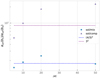Fig. 1 Ratio of virial parameters from the simulations of Federrath & Klessen (2012, Federrath & Klessen 2013) for three different types of forcing. Each point corresponds to a Mach number, ℳ, and size L. Triangles (sol/comp) show the ratio between virial parameters for solenoidal (b ≃ 0.3) and compressive forcing (b ≃ 1) and circles (sol/mix) show the ratio between solenoidal and mixed forcing (b ≃ 0.4). The horizontal dashed lines give the expected value of th e ratios for a scaling in b−2.

4 Conclusion

In this article we have applied the statistical formalism developed in Paper I to the determination of the total gravitational energy and virial parameter of a cloud. We have demonstrated that the contribution of the (undetermined) internal structure of the clouds has only a small impact on these determinations in clouds that are not in a too advanced stage of star formation. This is the case, for example, for the clouds Polaris and Orion B studied in Paper I. In that case, the cloud gravitational energy and virial parameter can thus be safely estimated from the observed total mass and size, with no knowledge of their internal structures. We, note, however that for clouds within which star formation has already been ongoing for a significant amount of time, that is when gravity has started to break the clouds into small isolated condensed regions, contributions from the internal structure can become sizeable and affect the estimate of the potential energy, e_G (see Sect. 2.1). This is an important result because the virial parameter determines the dynamics of a cloud, equilibrium, expansion or gravitational contraction.

Examining the same problem in a torus geometrical configuration, which is characteristic of numerical simulations in a periodic box, we have shown that, in contrast to real space, only the inner structure of the density fluctuations in the box contributes to the determination of the gravitational potential and the virial parameter (see Sect. 2.2). In that case, the (dominant) average contribution is lacking, a consequence of the ill-posed problem of solving the Poisson equation in ${\mathbb{T}}^3$. We have demonstrated that, for pure (initial) turbulent conditions, the ratio of the viral parameter values in the box over the ones in real geometry is proportional to ((l_c/L) × (bℳ))⁻² (Eq. (39)). Thus, for a given large-scale Mach number and size of the simulation box, this decreases approximately as ~b⁻², where b ∈ [1/3,1] denotes the (solenoidal vs compressive) turbulence forcing parameter. This explains the puzzling large discrepancy found in Federrath & Klessen (2012, Federrath & Klessen 2013) between the gravitational potential and virial parameter values inferred from the global characteristics of the simulation box and those inferred from the numerical results (see Sect. 3). We note that this does not affect the validity of the simulations of Federrath & Klessen (2012, Federrath & Klessen 2013). However, it does call for a reexamination of the interpretations that involve the estimation of α_vir from the gravitation potential returned by the simulations.

Finally, we remark that these findings only hold for clouds that are statistically homogeneous (see Paper I) and large enough compared to the correlation length of ρ. They notably do not hold for (small-scale) collapsed subregions.

These calculations highlight again the power of the statistical formalism developed in Paper I to explore the general statistical properties of star-forming MCs from a limited number of observations or simulations. As explored in the present paper, its power is notably significant when estimating its global gravitational energy and virial parameter, and thus the level of binding, of such MCs. These results will be used in a forthcoming paper aimed at exploring the evolution of the PDF in star-forming clouds.

Acknowledgements

The authors are grateful to Christoph Federrath for always providing data from his numerical simulations upon request.

Appendix A Computation of the total potential energy on a control volume Ω

We derive the gravitational binding energy of a cloud covering a domain Ω in Sect. (2), and divided it into three contributions to isolate the effects of the internal structure (deviation from the average): $$\langle e_G\left(\langle \rho \rangle \right)\rangle ={\displaystyle {\int }_{{\text{Ω}}^2}\frac{{\langle \rho \rangle }^2}{\left|\text{Ω}\right|}{\text{Φ}}_{\text{Green}}\left(x-x^{\prime }\right)\text{d}{x}^{\prime }}\text{\hspace{0.17em}d}x,$$(A.1) $$I_{C\left(\rho \right)}={\displaystyle {\int }_{{\text{Ω}}^2}\frac{\delta \rho \left(x\right)\delta \rho \left(x^{\prime }\right)}{\left|\text{Ω}\right|}{\text{Φ}}_{\text{Green}}\left(x-x^{\prime }\right)\text{d}{x}^{\prime }}\text{\hspace{0.17em}d}x,$$(A.2) $$2\langle \rho \rangle I_{\delta }\left(\rho \right)=2\langle \rho \rangle {\displaystyle {\int }_{{\text{Ω}}^2}\frac{\delta \rho \left(x\right)}{\left|\text{Ω}\right|}{\text{Φ}}_{\text{Green}}\left(x-x^{\prime }\right)}\text{\hspace{0.17em}d}{x}^{\prime }\text{\hspace{0.17em}d}x.$$(A.3)

Then, using the change in variables (u, v) = φ(x, x2) = (x −x2, x + x2), we obtain $$\langle e_G\left(\langle \rho \rangle \right)\rangle =\langle \rho \rangle {\displaystyle {\int }_{{\phi }_1\left(\text{Ω}\right)}\text{d}u{\text{Φ}}_{\text{Green}}\left(u\right)}{\displaystyle {\int }_{{\phi }_2^u\left(\text{Ω}\right)}\langle \rho \rangle }\frac{\text{d}\upsilon }{8\left|\text{Ω}\right|},$$(A.4) $$\begin{array}{lll}{I}_C\left(\rho \right)\hfill & =\hfill & {\displaystyle {\int }_{{\phi }_1\left(\text{Ω}\right)}\text{d}u{\text{Φ}}_{\text{Green}}\left(u\right)}{\displaystyle {\int }_{{\phi }_2^u\left(\text{Ω}\right)}\frac{\text{d}\upsilon }{8\left|\text{Ω}\right|}}\delta \rho \left(\frac{u+\upsilon }{2}\right)\delta \rho \left(\frac{u-\upsilon }{2}\right)\hfill \\ \hfill & =\hfill & {\displaystyle {\int }_{{\phi }_1\left(\text{Ω}\right)}\text{d}u{\text{Φ}}_{\text{Green}}\left(u\right)}{\widehat{C}}_{\rho ,L}\left(u\right),\hfill \end{array}$$(A.5) $$I\delta \left(\rho \right)={\displaystyle {\int }_{{\phi }_2^u\left(\text{Ω}\right)}\text{d}u{\text{Φ}}_{\text{Green}}\left(u\right)}{\displaystyle {\int }_{{\phi }_2^u\left(\text{Ω}\right)}\frac{\text{d}\upsilon }{8\left|\text{Ω}\right|}\delta \rho \left(\frac{u+\upsilon }{2}\right),}$$(A.6)

due to the fact that Ω possess a center of symmetry and where $${\phi }_1\left(\text{Ω}\right)=2\text{Ω},$$(A.7) $${\phi }_2^u\left(\text{Ω}\right)=2\left(\left(\text{Ω}-u\right)\cap \text{Ω}\right)+u,$$(A.8)

and ${\widehat{C}}_{\rho ,L}$ is the biased ergodic estimator of the ACF of ρ (see Sect. (2.1.2) and Appendix (A) of Paper I). For example, if $\text{Ω}={\left[-\frac{L}{2},\frac{L}{2}\right]}^3$ then ${\phi }_2^u\left(\text{Ω}\right)=\left[-L+\left|u_i\right|,L-\left|u_i\right|\right]]$.

Furthermore, denoting $$I\left(u\right)={\displaystyle {\int }_{{\phi }_2^u\left(\text{Ω}\right)}\frac{\text{d}\upsilon }{8\left|\text{Ω}\right|}\delta \rho \left(\frac{u+\upsilon }{2}\right)},$$(A.9)

we see that I(u) is, modulo the factor 1/|Ω|, the average of the density deviations, δρ, in the sub-volume ((Ω − u) ∩ Ω) + u/2. This is easier to see in the pedagogical case where $\text{Ω}={\left[-\frac{L}{2},\frac{L}{2}\right]}^3$ as $$\begin{array}{ll}I\left(u\right)\hfill & ={\displaystyle \int {\displaystyle \int {\displaystyle {\int }_{-L+\left|u_i\right|}^{L-\left|u_i\right|}\frac{\text{d}\upsilon }{8\left|\text{Ω}\right|}\delta \rho \left(\frac{u+\upsilon }{2}\right)}}}\hfill \\ \hfill & =\frac{1}{\left|\text{Ω}\right|}{\displaystyle \int {\displaystyle \int {\displaystyle {\int }_{\frac{-L+\left|u_i\right|+u_i}{2}}^{\frac{L-\left|u_i\right|+u_i}{2}}\delta \rho \left(x\right)}\text{\hspace{0.17em}d}x}.}\hfill \end{array}$$(A.10)

Then, if the volume of ((Ω − u) ∩ Ω) is sufficiently large, for example | ((Ω − u) n Ω) | ≫ l_c(ρ)³, I(u) ≃ | ((Ω − u) ∩ Ω) | 〈δρ〉 = 0 and $$I\left(u\right)\ll {\displaystyle {\int }_{{\phi }_2^u\left(\text{Ω}\right)}\langle \rho \rangle }\frac{\text{d}\upsilon }{8\left|\text{Ω}\right|}=\langle \rho \rangle \frac{\left|\left(\left(\text{Ω}-u\right)\cap \text{Ω}\right)\right|}{\left|\text{Ω}\right|}.$$(A.11)

The integral I(u) thus only gives non-negligible contributions for u in a small volume of order l_c(ρ)³ near the border ∂(2Ω), such as | ((Ω − u) ∩ Ω) | ≲ lc(p)³.

Therefore, providing that L = |Ω|^1/3 ≫ l_c(ρ), we can neglect 2 〈 ρ 〉 I_δ(ρ) with respect to 〈e_G(〈ρ 〉)〉. This leaves $$\langle e_G\rangle \simeq \langle e_G\left(\langle \rho \rangle \right)\rangle +{\displaystyle {\int }_{{\phi }_1\left(\text{Ω}\right)}\text{d}u{\text{Φ}}_{\text{Green}}\left(u\right)}{\widehat{C}}_{\rho ,L}\left(u\right).$$(A.12)

References

All Figures

Fig. 1 Ratio of virial parameters from the simulations of Federrath & Klessen (2012, Federrath & Klessen 2013) for three different types of forcing. Each point corresponds to a Mach number, ℳ, and size L. Triangles (sol/comp) show the ratio between virial parameters for solenoidal (b ≃ 0.3) and compressive forcing (b ≃ 1) and circles (sol/mix) show the ratio between solenoidal and mixed forcing (b ≃ 0.4). The horizontal dashed lines give the expected value of th e ratios for a scaling in b−2.

In the text

References

- Federrath, C. 2016, MNRAS, 457 375 [Google Scholar]
- Federrath, C., & Klessen, R. S. 2012, ApJ, 761 156 [Google Scholar]
- Federrath, C., & Klessen, R. S. 2013, ApJ, 763 51 [Google Scholar]
- Federrath, C., Klessen, R. S., & Schmidt, W. 2008, ApJ, 688, L79 [NASA ADS] [CrossRef] [Google Scholar]
- Federrath, C., Roman-Duval, J., Klessen, R., Schmidt, W., & Mac Low, M.-M. 2010, A&A, 512, A81 [NASA ADS] [CrossRef] [EDP Sciences] [Google Scholar]
- Guillet, T., & Teyssier, R. 2011, J. Comput. Phys., 230 4756 [Google Scholar]
- Jaupart, E., & Chabrier, G. 2020, ApJ, 903, L2 [NASA ADS] [CrossRef] [Google Scholar]
- Jaupart, E., & Chabrier, G. 2021a, ApJ, 922, L36 [NASA ADS] [CrossRef] [Google Scholar]
- Jaupart, E., & Chabrier, G. 2021b, A&A, 663, A113 (Paper I) [Google Scholar]
- Kritsuk, A. G., Norman, M. L., Padoan, P., & Wagner, R. 2007, ApJ, 665 416 [NASA ADS] [CrossRef] [Google Scholar]
- McKee, C. F., & Ostriker, E. C. 2007, ARA&A, 45 565 [Google Scholar]
- McKee, C. F., & Zweibel, E. G. 1992, ApJ, 399 551 [CrossRef] [Google Scholar]
- Ricker, P. 2008, ApJS, 176 293 [NASA ADS] [CrossRef] [Google Scholar]
The usual definition of the binding energy involves a 1/2 multiplying factor in order to account for summations on interacting pairs, which we omit here for the sake of clarity.
We recall that we omitted the usual factor 1/2 in the definition of the binding energy.