© The Authors 2023

1. Introduction

Turbulence is one of the key processes that shapes the spatial and temporal evolution of matter and energy across nearly all scales, from the laboratory up to astrophysical scales. When associated with the interstellar medium (ISM), turbulence is observed to lie in the supersonic regime (see for example Elmegreen & Scalo 2004; Mac Low & Klessen 2004; McKee & Ostriker 2007; Hennebelle & Falgarone 2012, and references therein), yielding coupled correlations between velocity and density fluctuations at all scales. Therefore, a physical model for predicting the spatial organisation of the gas density (and its tracers) throughout the ISM needs to account for the interactions between the velocity and density fields. This constitutes one of the open challenges in the astrophysics community and has key relevance for understanding the structure and dynamics of the ISM, and in particular the physical conditions for the formation of stars (Padoan et al. 2014).

There has been significant progress in the statistical characterisation of density fluctuations inferred from either observations or numerical simulations of the ISM. One of the most popular statistical tool is the one-point probability density function as it comes as input in several star formation models (Padoan & Nordlund 2002, 2011; Krumholz & McKee 2005; Hennebelle & Chabrier 2008; Federrath & Klessen 2012; Burkhart & Mocz 2019; Appel et al. 2022). It has been shown that for an isothermal gas in supersonic turbulence, the volume- and mass-weighted density fluctuations comply relatively well with a log-normal distribution. The latter arises naturally by assuming a random multiplicative process and the application of the central limit theorem for the density evolution (Vazquez-Semadeni 1994; Passot & Vázquez-Semadeni 1998; Kritsuk et al. 2007; Federrath et al. 2008, 2010). Significant deviations from the log-normal distribution are however observed when gravity (see for instance Kritsuk et al. 2011; Federrath & Klessen 2013; Girichidis et al. 2014; Khullar et al. 2021), magnetic fields, and/or stellar feedback (see for instance Krumholz et al. 2012; Myers et al. 2014; Kainulainen et al. 2014; Federrath 2015; Schneider et al. 2016) are included.

More insights into the spatial distribution of matter in the ISM can be provided by probing the microstructure of the density field. By microstructure, we refer here to any scale-dependent features of the density field and its tracers (the reader may refer to Elmegreen & Scalo 2004, for a complete review of several micro-structural descriptors). Such analysis can be carried out using two-point statistics: for example, correlation functions, structure functions, Fourier spectra or Δ-variance techniques, or principal component analysis (see for instance Stutzki et al. 1998; Ossenkopf & Mac Low 2002; Padoan et al. 2004; Heyer & Brunt 2004; Kim & Ryu 2005; Kritsuk et al. 2006; Federrath et al. 2010; Roman-Duval et al. 2010). The micro-structural content of the density field can also be assessed using geometrical approaches, which include fractal techniques (Elmegreen & Falgarone 1996; Stutzki et al. 1998; Federrath et al. 2009; Audit & Hennebelle 2010; Kritsuk et al. 2007; Beattie et al. 2019a,b) or multi-fractal spectra (Chappell & Scalo 2001). Independent of the tool, one generally seeks to find some power-law variations of the observable with respect to the scale. This power-law behaviour is very useful to spark phenomenological scenarios that describe the physics at play in the structural evolution of the gas density in the ISM. However, the existence of some power laws is generally observed, sometimes predicted using dimensional arguments, but it is not generally derived from first principles. One attempt to fill this gap is presented by Galtier & Banerjee (2011) and Ferrand et al. (2020) who derived the exact generalised Kolmogorov equation directly from the compressible Navier-Stokes equations. The work by Aluie (2013) also provides some theoretical insights into the scale distribution of compressible turbulence based on the coarse grained Navier-Stokes equations. Nevertheless, such exact scale-by-scale budget equations, although extremely valuable to describe the physics at play, still require some closures for being used as a predictive tool.

In the present study, we aim to provide new insights into the role of supersonic turbulence in determining the spatial structure of the gas density in the ISM. We propose using a two-point statistical analysis of the phase indicator field defined from different density thresholds. Such an approach is encountered in other branches of physics, dealing with for example, heterogeneous materials (Adler et al. 1990; Torquato 2002; Teubner 1990; Kirste & Porod 1962; Frisch & Stillinger 1963; Berryman 1987) or fractal aggregates (Sorensen 2001; Morán et al. 2019). Its application to fluid mechanics is relatively scarce, although it has been applied with success in single-phase turbulence (Hentschel & Procaccia 1984; Vassilicos & Hunt 1991, 1996; Vassilicos 1992; Elsas et al. 2018; Gauding et al. 2022) and multiphase turbulent flows (Lu & Tryggvason 2018, 2019; Thiesset et al. 2020, 2021). There are several theoretical results based on robust mathematical grounds allowing the two-point statistics of iso-value sets to be related to some geometrical and/or fractal properties. An exact transport equation for such two-point statistics was further derived (Thiesset et al. 2020; Gauding et al. 2022), which makes the interactions explicit between the probed field variable and the turbulent velocity field. It is therefore believed that this tool could be promising to investigate the density fluctuations in supersonic turbulence. Although virtually applicable to all scenarios involving turbulent flows, this framework was first appraised using data from a high-resolution simulation of supersonic isothermal turbulence (Federrath et al. 2021).

The rest of the paper is organised as follows. Section 2 gathers the main theoretical derivations. The numerical database and post-processing procedures are introduced in Sect. 3. Our results are presented in Sect. 4 and conclusions are drawn in Sect. 5.

2. A structural descriptor of iso-density sets

2.1. The phase indicator field

The analysis is based on the phase indicator function ϕ(x, t) defined as:

$$\begin{array}{c}\hfill \varphi (\mathit{x},t)=\{\begin{array}{c}1\mathrm{when}\rho (\mathbf{x},\mathrm{t})>{\rho }_{\mathrm{th}}\hfill \\ 0\mathrm{otherwise}.\hfill \end{array}\end{array}$$(1)

This quantity reads as the probability that the density ρ is larger than a certain threshold ρ_th at a given position in space x and time t. It is also sometimes referred to as the excursion set or here iso-density set. The phase indicator function was introduced notably to characterise heterogeneous media such as composite materials and/or porous media (see for instance Debye et al. 1957; Porod 1951). Such fields are discontinuous by nature with two (or more) phases separated by an interface. In supersonic turbulence, the presence of shocks may lead also to local discontinuities of the density field. Despite, one can always define a phase indicator field, in the presence or absence of discontinuities, and hence it is applicable here to the density field, even in presence of shocks.

Investigating the properties of ϕ(x, t) for different iso-values ρ_th allows the geometry of the density field to be characterised. Low and high values of ρ_th correspond the dilute and dense regions, respectively. The relevant geometrical properties of ϕ investigated here are detailed below.

The first quantity is the volume fraction, which is simply defined as the ratio between the phase indicator volume and the averaging volume:

$$\begin{array}{c}\hfill ⟨\varphi ⟩=\frac{1}{V}{\displaystyle \int }\varphi (\mathit{x},t)\mathrm{d}V.\end{array}$$(2)

The brackets in Eq. (2) denote a volume average over the volume V. The volume fraction ⟨ϕ⟩ has no units and is comprised between 0 and 1.

The second relavant geometrical feature of the field ϕ is the surface density, which represents the surface area of the interface separating ϕ = 1 and ϕ = 0, divided by the averaging volume:

$$\begin{array}{c}\hfill \mathrm{\Sigma }=⟨|\mathbf{\nabla }\varphi (\mathit{x},t)|⟩=\frac{1}{V}{\displaystyle \int }|\mathbf{\nabla }\varphi (\mathit{x},t)|\mathrm{d}V.\end{array}$$(3)

We note that in the astrophysics community, the surface density generally refers to the cloud mass divided by the cloud bounding surface area. It is thus given in units of mass per area. Let this quantity be noted Σ_m. In Eq. (3), what we call surface density Σ, is a purely geometrical quantity with no connection to the mass, defined by the area of the iso-density surface divided by the averaging volume. Hence, it is in units of inverse of length. Consequently, for a cloud with fixed mass, if its bounding surface increases, the mass surface density Σ_m decreases while, the geometrical surface density Σ increases. Therefore, they evolve in opposite directions. One possible way to relate these two quantities is to compute the mass fraction ⟨ρϕ⟩ (that is the mass contained in the iso-volume defined by ρ(x, t) > ρ_th divided by the averaging volume V) and then one has Σ_m = ⟨ρϕ⟩/Σ.

We can go beyond and compute the statistics of the spatial increment for ϕ, which is written δϕ and is defined as the difference of ϕ between two points x + r and x, arbitrarily separated in space by a distance r:

$$\begin{array}{c}\hfill \delta \varphi (\mathit{r},t)=\varphi (\mathit{x}+\mathit{r},t)-\varphi (\mathit{x},t).\end{array}$$(4)

We consider in particular the second-order moment of δϕ, also called the second-order structure function, defined by:

$$\begin{array}{c}\hfill ⟨{(\delta \varphi )}^2⟩=\frac{1}{V}{\displaystyle \int }{(\delta \varphi )}^2\mathrm{d}V.\end{array}$$(5)

The phase indicator function can also be studied through its two-point correlation function defined as:

$$\begin{array}{c}\hfill ⟨{\varphi }_m^{+}{\varphi }_m⟩=\frac{1}{V}{\displaystyle \int }{\varphi }_m(\mathit{x}+\mathit{r}){\varphi }_m(\mathit{x})\mathrm{d}V.\end{array}$$(6)

The + superscript in Eq. (6) is used to denote that the quantity is taken at point x + r while ϕ_m denotes the phase indicator for the minority phase at point x. The minority phase is defined by

$$\begin{array}{c}\hfill {\varphi }_m(\mathit{x},t)=\{\begin{array}{c}\varphi (\mathit{x},t)\mathrm{if}⟨\varphi ⟩\le 0.5\hfill \\ 1-\varphi (\mathit{x},t)\mathrm{if}⟨\varphi ⟩>0.5.\hfill \end{array}\end{array}$$(7)

We thus have ⟨ϕ_m⟩=min(⟨ϕ⟩,1 − ⟨ϕ⟩). The majority phase is defined as the complementary set of the minority phase and is equal to ϕ′ = 1 − ϕ_m. Contrary to the autocorrelation function, the second-order structure function is the same when computed from the majority or minority phase.

Thiesset et al. (2020) derived the relation between the correlation function and the second-order structure function:

$$\begin{array}{c}\hfill \frac{⟨{\varphi }_m^{+}{\varphi }_m⟩}{⟨{\varphi }_m⟩}=1-\frac{⟨{(\delta \varphi )}^2⟩}{2⟨{\varphi }_m⟩}.\end{array}$$(8)

Although Eq. (8) reveals that the correlation and structure function are intimately linked, we subsequently show later in this paper that they provide different information about the system.

In general (inhomogeneous and anisotropic) situations, both the second-order structure function ⟨(δϕ)²⟩ and the correlation function $\langle {\varphi }_m^{+}{\varphi }_m\rangle$ depend on the 3-dimensional separation vector r and the 3-dimensional position vector x. Homogeneity can be invoked such that two-point statistics are invariant by translation, thereby dropping the dependence to the vector x. In case of isotropic media, two-point statistics depend only on the modulus of the separation vector r ≡ |r|. The numerical data detailed in Sect. 3 and discussed in Sect. 4 correspond to homogeneous and isotropic turbulence, which means that the two-point statistics discussed hereafter are function of r, only.

The framework presented here was used in its fully inhomogeneous and anisotropic version in Thiesset et al. (2021). These authors showed that the relations to be discussed below apply to the ‘homogeneised’ (after application of a spatial average) and ‘isotropised’ (after application of an angular average over all orientations of the separation vector) version of the original inhomogeneous and anisotropic media.

2.2. Asymptotic behaviour of two-point statistics

The asymptotic behaviour of ⟨(δϕ)²⟩ and $\langle {\varphi }_m^{+}{\varphi }_m\rangle$ for different range of scales are known and are detailed below.

2.2.1. At small scales

Since ϕ can take only 1 or 0 values, we have ϕ² ≡ ϕ, and hence the correlation function $\langle {\varphi }_m^{+}{\varphi }_m\rangle$ at r = 0 is given by

$$\begin{array}{c}\hfill ⟨{\varphi }_m^{+}{\varphi }_m⟩(r=0)=⟨{\varphi }_m⟩.\end{array}$$(9)

Therefore, the correlation function at r = 0 gives information about the volume fraction of the minority phase ⟨ϕ_m⟩. The second-order structure function ⟨(δϕ)²⟩ is 0 at r = 0.

The asymptotic regime when the separation r tends to zero was derived by Porod (1951), Guinier et al. (1955), and Debye et al. (1957), who proved that for homogeneous isotropic media:

$$\begin{array}{c}\hfill \underset{r\to 0}{lim}⟨{\varphi }_m^{+}{\varphi }_m⟩=⟨{\varphi }_m⟩-\frac{\mathrm{\Sigma }r}{4}.\end{array}$$(10)

This implies for ⟨(δϕ)²⟩ the following limit:

$$\begin{array}{c}\hfill \underset{r\to 0}{lim}⟨{(\delta \varphi )}^2⟩=\frac{\mathrm{\Sigma }r}{2}.\end{array}$$(11)

Equations (10) and (11) can be seen as the 3D extension of the classical Buffon needle problem. It shows that if the interface between ϕ = 1 and ϕ = 0 becomes planar when observed at sufficiently small scales, the probability that the two points x and x + r lie on each side of the interface is then simply proportional to the surface density Σ and the distance |r| between the two points. Equations (10) and (11) remain valid in anisotropic media when two-point statistics are angularly averaged over all orientations of the vector r (Berryman 1987). This linear regime is observed only if the interface is planar at some resolution scales. In case of purely fractal sets, revealing rough interfaces at all scales, this regime is not likely to be observed.

2.2.2. At larger, yet small scales

For slightly larger values of the separation r, the curvature of the interface becomes perceptible, and one needs to account for the next terms in the small-scale expansion of $\langle {\varphi }_m^{+}{\varphi }_m\rangle$ and ⟨(δϕ)²⟩. These were first derived by Kirste & Porod (1962) and Frisch & Stillinger (1963), and later by Teubner (1990) and Ciccariello (1995), and read:

$$\begin{array}{c}\hfill \underset{r\to 0}{lim}⟨{\varphi }_m^{+}{\varphi }_m⟩=⟨{\varphi }_m⟩-\frac{\mathrm{\Sigma }r}{4}(1-{⟨C⟩}_{\mathrm{s}}\frac{r^2}{8}).\end{array}$$(12)

By virtue of Eq. (8), we then have for ⟨(δϕ)²⟩:

$$\begin{array}{c}\hfill \underset{r\to 0}{lim}⟨{(\delta \varphi )}^2⟩=\frac{\mathrm{\Sigma }r}{2}(1-{⟨C⟩}_{\mathrm{s}}\frac{r^2}{8}).\end{array}$$(13)

The quantity ⟨C⟩_s in Eqs. (12) and (13) is related to the mean and Gaussian curvature, denoted H and G:

$$\begin{array}{c}\hfill {⟨C⟩}_{\mathrm{s}}=[{⟨H^2⟩}_{\mathrm{s}}-\frac{{⟨G⟩}_{\mathrm{s}}}{3}],\end{array}$$(14)

where ⟨ • ⟩_s denotes a surface-area-weighted average: ⟨ • ⟩_sΣ = ⟨ • |∇ϕ|⟩. Eqs. (12) and (13) reveal that the quantity $1/{⟨C⟩}_{\mathrm{s}}^{1/2}$ can be associated with the transition scale where the interface starts being curved. In anisotropic media, Eq. (13) was shown to hold true when an angular average is applied on two-point statistics (Thiesset et al. 2021).

2.2.3. In the intermediate range of scales

The correlation and structure functions are known to provide information about the fractal features of the object, if any. As stated for example by Sreenivasan et al. (1989), an object is likely to exhibit a fractal scaling in a range of scales lying between an inner cutoff η_i (here a scale somehow related to ${⟨C⟩}_{\mathrm{s}}^{-1/2}$) and an outer cutoff η_o (a kind of integral length-scale). If the separation between η_i and η_o is sufficiently large, then one should expect $\langle {\varphi }_m^{+}{\varphi }_m\rangle$ and/or ⟨(δϕ)²⟩ to follow a power law with an exponent that can be related to the fractal dimension.

However, in this context, it is important to make the distinction between what is referred to as a mass-fractal and a surface-fractal. Schematically, a mass-fractal is an object whose bulk reveals some fractal features while its surface remains smooth. Soot aggregates issued from combustion of hydrocarbon fuels typically fall in this category (Sorensen 2001; Morán et al. 2019). Such an object is presented in Fig. 1a. It is composed of a set of small spherical particles with constant density whose surface is smooth, and assembles to form an object with fractal features. Another example is the Menger sponge as illustrated in Fig. 1c. The latter is composed of perforated cubes with scale-similarity. Except at the corners, its surface is always planar.

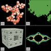Fig. 1. Illustrations of different categories of fractals. Examples of mass-fractals: (a) a soot particle and (c) the Menger sponge. Examples of surface-fractals : (b) a coastline and (d) the Julia set.

A surface-fractal is the opposite: an object whose body remains compact while its surface is fractal. Some examples are given in the right column of Fig. 1. Figure 1b shows a coastline, and the Julia set is illustrated in Fig. 1d, which are examples of typical surface-fractals.

This distinction is of major importance here since the correlation and structure function for mass- and surface-fractals exhibit different behaviour in the intermediate range of scales. Indeed, for instance Sorensen (2001) and Wong & Cao (1992) (and references therein) mentioned that for mass-fractals:

$$\begin{array}{c}\hfill ⟨{\varphi }_m^{+}{\varphi }_m⟩\sim r^{{\xi }_m},\end{array}$$(15)

where ξ_m = D_m − 3 with D_m the mass-fractal dimension.

By contrast, for surface-fractals (Wong & Cao 1992) with dimension D_s:

$$\begin{array}{c}\hfill ⟨{\varphi }_m^{+}{\varphi }_m⟩=⟨{\varphi }_m⟩-K{r}^{{\xi }_{\mathrm{s}}},\end{array}$$(16)

where ξ_s = 3 − D_s, and K is a constant. Equation (16) together with Eq. (8) indicates that:

$$\begin{array}{c}\hfill ⟨{(\delta \varphi )}^2⟩\sim r^{{\xi }_{\mathrm{s}}}.\end{array}$$(17)

Therefore, probing the scale dependence of $\langle {\varphi }_m^{+}{\varphi }_m\rangle$ and ⟨(δϕ)²⟩ separately enables (i) to assess whether the object under consideration is rather a mass- or surface-fractal, and (ii) to estimate the corresponding dimension D_m or D_s.

An example is given in Fig. 2 where we have computed $\langle {\varphi }_m^{+}{\varphi }_m\rangle$ and ⟨(δϕ)²⟩ for the Menger sponge (a mass-fractal) and the Julia set (a surface-fractal). For the Julia set, ⟨(δϕ)²⟩ reveals an appreciable power-law range, while no such behaviour is observed for $\langle {\varphi }_m^{+}{\varphi }_m\rangle$. The opposite is observed for the Menger sponge. In each situation the computed power-law exponent complies well with the theoretical values of D_m = log₃(20)≈2.73 and D_s ≈ 2.27 for the Menger sponge and the Julia set, respectively. It is worth noting that in Fig. 2, ⟨(δϕ)²⟩ does not reveal any range of scales complying with a linear regime with respect to the separation r (Eq. (11)). This means that the Julia and Menger sets are rough at all scales.

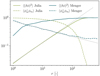Fig. 2. Correlation and structure function for the Menger sponge and the axisymmetric Julia set (z ⇌ z2 − 1). The grey dotted line represents the theoretical power laws with Dm = log3(20) for the Menger sponge and Ds ≈ 2.27 for the Julia set.

The distinction between mass- and surface-fractal yields important consequences. In particular, the mass–size distribution for mass-fractals is

$$\begin{array}{c}\hfill M(r)\sim r^{D_m},\end{array}$$(18)

while for surface fractals,

$$\begin{array}{c}\hfill M(r)\sim r^3.\end{array}$$(19)

For a surface-fractal, the surface area measured at scale r (known as the surface-scale distribution) is given by (Sreenivasan et al. 1989; Wong & Cao 1992)

$$\begin{array}{c}\hfill S(r)\sim r^{D_{\mathrm{s}}-2}.\end{array}$$(20)

One can further imagine a situation where a mass-fractal is bounded by a surface-fractal. In this case, Wong & Cao (1992) obtained that:

$$\begin{array}{c}\hfill M(r)\sim r^{D_m}(1-A{\left(\frac{r}{R}\right)}^{3-D_{\mathrm{s}}})\end{array}$$(21)

for any r < R where R³ is the volume enclosed by the surface given by ⟨ϕ_m⟩=R³/V, and A is a constant of order unity. It is noted that the correction A(r/R)^{3 − D_s} is perceptible only at scales close to R.

2.2.4. At large scales

The asymptotic limit of the correlation function at large scales is

$$\begin{array}{c}\hfill \underset{r\to \infty }{lim}⟨{\varphi }_m^{+}{\varphi }_m⟩={⟨{\varphi }_m⟩}^2.\end{array}$$(22)

This result implies that for the second-order structure function (Thiesset et al. 2020, 2021; Gauding et al. 2022):

$$\begin{array}{c}\hfill \underset{r\to \infty }{lim}⟨{(\delta \varphi )}^2⟩=2⟨\varphi ⟩(1-⟨\varphi ⟩)\end{array}$$(23)

Hence, in the limit of large scales, both $\langle {\varphi }_m^{+}{\varphi }_m\rangle$ and ⟨(δϕ)²⟩ give information about the volume fraction.

2.2.5. Summary of the schematic representation of ϕ

These different asymptotic regimes are schematically summarised in Fig. 3. This figure shows that when probed at asymptotically small scales, the interface seems planar. In this regime, ⟨(δϕ)²⟩ and $\langle {\varphi }_m^{+}{\varphi }_m\rangle$ are intimately linked to the surface density Σ. At slightly larger scales, that is for scales r ∼ ⟨C⟩^−1/2, the interface curvature starts to become visible. Both ⟨(δϕ)²⟩ and $\langle {\varphi }_m^{+}{\varphi }_m\rangle$ are then given by Eqs. (13) and (12), respectively. If r lies well between η_i and η_o, then a fractal scaling can possibly be observed. In this situation ⟨(δϕ)²⟩ follows a power law with an exponent ξ_s = 3 − D_s if the object is surface-fractal. Conversely, if the object is mass-fractal, then the correlation function exhibits a power law with exponent ξ_m = D_m − 3. Finally, at large scales, ⟨(δϕ)²⟩ starts being a volumetric descriptor and reaches the asymptotic value of 2⟨ϕ⟩(1 − ⟨ϕ⟩), while $\langle {\varphi }_m^{+}{\varphi }_m\rangle$ tends towards ⟨ϕ_m⟩².

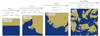Fig. 3. Schematic representation of the different asymptotic regimes of ⟨(δϕ)2⟩ and $\langle {\varphi }_m^{+}{\varphi }_m\rangle$ for different scale ranges from small to large scales.

As an overall conclusion, the quantities ⟨(δϕ)²⟩ and $\langle {\varphi }_m^{+}{\varphi }_m\rangle$ contain information about the surface density, the interface curvature, the fractal characteristics and the volume fraction. All these quantities are important geometric measures that are contained in and characterised by the rather simple structural descriptor ϕ defined in Eq. (1).

2.3. Scale-by-scale budget

The analysis based on the correlation and structure functions of the phase indicator ϕ can be supplemented by a transport equation, which is known as a scale-by-scale budget. When applied to the density field (a conserved quantity), the time and space evolution of ϕ is given by (Thiesset et al. 2020, 2021; Gauding et al. 2022),

$$\begin{array}{c}\hfill {\partial }_t\varphi +\mathit{u}·\mathbf{\nabla }\varphi =0,\end{array}$$(24)

where u is the fluid velocity at the interface. Using the machinery described by Thiesset et al. (2020) and Gauding et al. (2022), one can derive the transport equation for ⟨(δϕ)²⟩ (and $\langle {\varphi }_m^{+}{\varphi }_m\rangle$). The general scale-by-scale budget for reacting and diffusive quantities evolving in non-stationary, inhomogeneous, anisotropic, possibly compressible flows is provided by Gauding et al. (2022). Here we provide the formulation for a statistically homogeneous and stationary flow, as in our numerical simulations. In this case, the equation for ⟨(δϕ)²⟩ simplifies to

$$\begin{array}{c}\hfill {\mathbf{\nabla }}_{\mathit{r}}·⟨(\delta \mathit{u}){(\delta \varphi )}^2⟩=2⟨{(\mathbf{\nabla }·\mathit{u})}^{\oplus }{(\delta \varphi )}^2⟩.\end{array}$$(25)

The quantity •^⊕ = (•⁺ + •)/2 is the arithmetic mean of the quantity • between the points x and x + r. The transport equation for the correlation function was obtained by Gauding et al. (2022). Equation (25) was derived by assuming that the velocity u is differentiable when crossing the interface. Hence, this formulation of scale-by-scale is restricted to cases where the velocity can be assumed to be smoothly varying on each side of the iso-density surface. In case of strong shocks, associated with discontinuous velocity jumps, the weak formulations of the scale-by-scale budgets, such as those discussed by Duchon & Robert (2000), Saw et al. (2016), Galtier (2018), Dubrulle (2019) for the turbulent kinetic energy, should be derived and used instead.

By further taking advantage of isotropy, the transfer term on the left-hand side of Eq. (25), which writes as the divergence in scale-space of the flux ⟨(δu)(δϕ)²⟩, can be expressed in spherical coordinates, which leads to:

$$\begin{array}{c}\hfill ⟨(\delta u_{\Vert }){(\delta \varphi )}^2⟩=\frac{2}{r^2}{\displaystyle {\int }_0^r{r}^2⟨{(\mathbf{\nabla }·\mathit{u})}^{\oplus }{(\delta \varphi )}^2⟩\mathrm{d}r.}\end{array}$$(26)

The quantity u_∥ = u ⋅ r/r is the longitudinal velocity: the velocity component in the direction of r.

Equation (26) is exact and is derived without any other hypothesis than the one invoked above (homogeneous, isotropic, stationary fields). It reveals the effect of velocity and velocity divergence on the evolution of the microstructure of the density field as measured through ⟨(δϕ)²⟩ or $\langle {\varphi }_m^{+}{\varphi }_m\rangle$ at a given threshold ρ_th. The term on the left-hand side of Eq. (26) is the scale-by-scale transport of the quantity ϕ by the velocity field. In the classical Kolmogorov (1941) or Yaglom (1949) theory, for incompressible turbulence and turbulent mixing, respectively (see also Danaila et al. 2004), this term is generally associated with the cascade process (see also Galtier & Banerjee 2011; Ferrand et al. 2020, for more recent derivations of a Kolmogorov-type theory of compressible isothermal turbulence). When negative, the flux of (δϕ)² is directed towards small scales (a direct cascade), while positive ⟨(δu_∥)(δϕ)²⟩> 0 is referred to as an inverse cascade from small to large scales.

The process on the right-hand side of Eq. (26) arises in flows with non-zero velocity divergence. When positive (negative), this process acts in expanding (contracting) the microstructure in the space of separation r. The velocity divergence is thus a sink/source term in the scale-by-scale budget of the iso-density field, which counteracts the transfer process. Very similar conclusions were drawn by Galtier & Banerjee (2011) and Ferrand et al. (2020), who showed that the divergence of the velocity acts similarly in the scale-by-scale budget for the velocity structure functions.

The asymptotic behaviour of the different terms in Eq. (26) at small scales was determined by Gauding et al. (2022). For the flux term, the limit is

$$\begin{array}{c}\hfill \underset{r\to 0}{lim}-⟨(\delta u_{\Vert }){(\delta \varphi )}^2⟩=\mathbb{K}\mathrm{\Sigma }\frac{r^2}{8},\end{array}$$(27)

where 𝕂 = ⟨ − n ⋅ ∇u ⋅ n⟩_s is here the tangential component of the strain rate acting on the iso-surface ρ(x, t) = ρ_th (Candel & Poinsot 1990). The vector n = −∇ϕ/|∇ϕ| is the unit normal vector to the interface. The other component of the strain rate writes ⟨∇ ⋅ u⟩_s and is due to the velocity divergence. This term arises from the limit of the term on the right-hand side of Eq. (26), in the limit of small separations:

$$\begin{array}{c}\hfill \frac{2}{r^2}{\displaystyle {\int }_0^r{r}^2⟨{(\mathbf{\nabla }·\mathit{u})}^{\oplus }{(\delta \varphi )}^2⟩\mathrm{d}r={⟨\mathbf{\nabla }·\mathit{u}⟩}_{\mathrm{s}}\mathrm{\Sigma }\frac{r^2}{8}.}\end{array}$$(28)

The turbulent flow that we subsequently investigate in the following, is at steady state. In this situation, the sum of the two components of the strain rate is zero.

3. Numerical setup and post-processing

Here we analyse data from a highly resolved numerical simulation of supersonic isothermal turbulence. The database and numerical methods used in this simulation are described in detail in Federrath et al. (2021; see also Ferrand et al. 2020). We briefly summarised the main methods below.

The compressible Euler equation in three dimensions:

$$\begin{array}{c}\hfill {\partial }_t\rho \mathit{u}+\mathbf{\nabla }·\rho \mathit{u}\otimes \mathit{u}=-\mathbf{\nabla }p+\rho \mathit{F},\end{array}$$(29)

is solved, together with the continuity equation

$$\begin{array}{c}\hfill {\partial }_t\rho +\mathbf{\nabla }·\rho \mathit{u}=0,\end{array}$$(30)

using the code FLASH (Fryxell et al. 2000; Dubey et al. 2008). These equations are solved on a triply periodic Cartesian mesh using a positivity-preserving MUSCL-Hancock HLL5R Riemann scheme (Waagan et al. 2011). An isothermal equation of state for a perfect gas, $p=\rho c_{\text{s}}^2$, is used to relate the pressure p and the density ρ through the sound speed c_s, which is constant. Turbulence statistics are maintained at steady state using a forcing ρF. The latter acts at large scales and is composed of a half solenoidal and half compressive mode, termed natural mixture in Federrath et al. (2010). The turbulence driving code is available on GitHub (Federrath et al. 2022). As in Federrath et al. (2021), the turbulent Mach number is defined as $\mathcal{M}=\sqrt{⟨{\mathit{u}}^2⟩/c_{\mathrm{s}}^2}$. Here, the Mach number is ℳ = 4.1. The grid consists of 10 048³ data points stored into 65 536 blocks of 157 × 314 × 314 points each. 5 snapshots separated by one eddy turnover time in the fully developed turbulent state were used to average the statistical measurements below.

The surface-scale relation to be described later is obtained from a standard method (de Silva et al. 2013; Hawkes et al. 2012; Thiesset et al. 2016; Krug et al. 2017). It consists first in coarse-graining the field variable of interest (here the density) at different filter size Δ. For each filter size, the phase indicator field can then be extracted by thresholding the filtered density field. By doing so, the surface area of the ‘filtered’ interface can be computed and studied as a function of Δ to determine the surface-scale relation.

Here, the filtered density denoted $\overline{\rho }$ is obtained by using a box average over a cubic sub-set of size Δ. We note that the transport equation for the filtered density is the same as the unfiltered one:

$$\begin{array}{c}\hfill {\partial }_t\overline{\rho }+\mathbf{\nabla }·\overline{\rho }\stackrel{\sim }{\mathit{u}}=0,\end{array}$$(31)

where the Favre-filtered velocity is given by:

$$\begin{array}{c}\hfill \stackrel{\sim }{\mathit{u}}=\frac{\overline{\rho \mathit{u}}}{\overline{\rho }}.\end{array}$$(32)

Therefore, the scale-by-scale budget (Eq. (26)) remains formally the same when the Favre-average velocity $\stackrel{\sim }{\mathit{u}}$ is used in place of u. We have investigated different ratios of filter size to the original grid spacing Δ_x, from Δ = Δ_x (the unfiltered case) to 32Δ_x, resulting in 6 down-sampled datasets composed of 314³, 628³, 1256³, 2512³, 5024³ and 10 048³ grid points for Δ/Δ_x = 32, 16, 8, 4, 2, 1.

The correlation and structure functions are computed using the library pyarcher (Thiesset & Poux 2020). Only spatial separations r aligned with the three Cartesian directions (e_x, e_y, e_z) were considered and subsequently averaged, taking advantage of isotropy. The separation vector was varying between 1 grid spacing up to half the simulation box size, which is identical to the turbulence driving scale, denoted L. The number of sampling pairs is given by 5 (snapshots) × 3 (directions) × 10 048³(Δ_x/Δ)³ (points), and was thus varying between about 10⁸ and 10¹³ for Δ between 32Δ_x and Δ_x, respectively. This was found sufficient to reach statistical convergence of the structure and correlation functions (cf., respective sampling tests for the structure functions in Federrath et al. 2021).

Seven different values for the density threshold ρ_th were chosen: ρ_th/ρ₀ = {0.1, 0.2, 0.5, 1, 2, 5, 10}. In the present simulation, the volume average density ρ₀ ≡ ⟨ρ⟩ = 1, and hence ρ_th will hereafter be given in units of ρ₀. The density and the corresponding phase indicator fields for varying ρ_th are portrayed in Fig. 4. We note that the density field is highly convoluted with some fluctuations ranging very different scales. When observed at large scales (at the size of the simulation box), dilute regions (ρ_th < 1) take the form of bulky and agglomerated structures, while dense regions (ρ_th > 1) are more sparse and filamentary. Neutral density (ρ_th ∼ 1) regions reveal some branched structures.

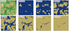Fig. 4. Two-dimensional slices of the density field and their associated phase indicator field. (a) slice of log(ρ/ρ0) with light (dark) colours corresponding to low (high) values. (b–h) Corresponding iso-density set with ρth = 0.1 to 10.0, as indicated in the legend of each panel. The yellow and blue regions correspond to ϕ = 0 and ϕ = 1, respectively.

4. Results

4.1. Volume fraction

Federrath et al. (2021) showed that the probability density function of ρ obtained from the present simulation data is well represented by the intermittency model distribution by Hopkins (2013). However, the value of the intermittency correction was found to be rather small. This suggests that the log-normal distribution provides a good approximation. Assuming that the volume-weighted probability density function of ρ is log-normal, one can easily derive the following expression for the volume fraction ⟨ϕ⟩:

$$\begin{array}{c}\hfill ⟨\varphi ⟩=\frac{1}{2}(1-\mathrm{erf}\left[\frac{log{\rho }_{\mathrm{th}}+\frac{1}{2}{\sigma }_{\mathrm{s}}^2}{\sqrt{2{\sigma }_{\mathrm{s}}^2}}\right]).\end{array}$$(33)

In Eq. (33), ‘erf’ is used to denote the error function and σ_s is the volume-weighted dispersion (standard deviation) of s = log ρ/ρ₀. Federrath et al. (2021) measured σ_s = 1.21 for this simulation.

Figure 5 gathers the numerical values for ⟨ϕ⟩ when the iso-density is varied from 0.1 to 10. The colour code for each iso-density value (light for low, dark for high ρ_th) will be followed in the sequel. The volume fraction is about 90% for ρ_th = 0.1 and decreases down to 5‰ for ρ_th = 10. The median ⟨ϕ⟩ = 0.5 is obtained for ${\rho }_{\text{th}}=\exp (-{\sigma }_{\text{s}}^2/2)\approx 0.48$. The prediction assuming a log-normal distribution, Eq. (33), compares favourably well to the numerical data, except maybe at low values of ρ_th where the intermittency correction starts to become significant. Figure 5 together with Eq. (33) shows that evaluating ⟨ϕ⟩ for different ρ_th is equivalent to evaluating the (cumulative) probability density function of ρ.

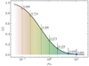Fig. 5. Volume fraction ⟨ϕ⟩ for the different values of ρth (symbols). The black solid line corresponds to the prediction of Eq. (33) with a dispersion parameter σs = 1.21.

4.2. Structure and correlation functions

We now analyse the structure function ⟨(δϕ)²⟩ for the unfiltered dataset. Results for iso-density values 0.1 ≤ ρ_th ≤ 10 are presented in Fig. 6. The inset represents the local scaling exponent ∂_log(r)log⟨(δϕ)²⟩. The sonic scale r_s = 0.025L which is the scale at which the local Mach number is equal to one (Federrath et al. 2021) is also represented. The structure function is normalised by 2⟨ϕ⟩(1 − ⟨ϕ⟩), whereas the separation r is normalised by L (the turbulence driving scale). We note that all curves converge to the same plateau when r → ∞ as expected from Eq. (23). The local scaling exponent is thus zero in this range of scales.

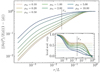Fig. 6. Scaling of ⟨(δϕ)2⟩ for Δ = 1Δx, that is N = 10 0483 and ρth from 0.1 to 10.0. The inset shows the local scaling exponent ∂log(r)log⟨(δϕ)2⟩. The grey dashed line represents the fit using Eq. (34). The sonic scale rs is shown by the vertical black dotted line.

Travelling through smaller scales, we note the onset of a power-law behaviour for ⟨(δϕ)²⟩. The latter is particularly visible for low ρ_th. For instance, the local scaling exponent is constant over more than a decade for ρ_th = 0.1. The power-law range is centred around the sonic scale. We further note that contrary to the velocity structure functions reported by Federrath et al. (2021), which reveal different scaling exponents below and above the sonic scale, the ϕ-field structure function exponent is roughly the same in the sub- and supersonic range. The observed power-law behaviour in the intermediate range of scales means that iso-density fields are surface-fractals (cf., Figs. 1 and 2). The value for the scaling exponent differs depending on the chosen iso-density threshold, which means that the density field cannot be described by a unique surface fractal dimension. Instead, the dimension D_s of iso-density sets increases with ρ_th. In other words, the fractal content of iso-density surfaces is larger for dense clumps than dilute regions.

When the separation r tends to smaller values, the structure function ⟨(δϕ)²⟩ ceases to follow a power law and the local scaling exponent progressively evolves to reach a value of 1 at very small scales. The scale at which this transition appears is roughly the same irrespective of ρ_th. This suggests that the inner cutoff, which is the scale below which the iso-surface stops being fractal, is independent of ρ_th. More details on this aspect will be given later when analysing the surface–size distribution. The fact that ⟨(δϕ)²⟩ follows a linear regime when r → 0 means that the iso-density surface is planar when observed at sufficiently small scales. This result is not so intuitive since in supersonic turbulence, the presence of shocks may yield a loss of smoothness of the density field at all scales. It is however unclear if this observed planarity of iso-density surfaces is ’physical’ or is due to numerical dissipation.

Gauding et al. (2022) found that ⟨(δϕ)²⟩ can be represented by the following parametric expression:

$$\begin{array}{c}\hfill ⟨{(\delta \varphi )}^2⟩(r)=\frac{\mathrm{\Sigma }r}{2}\frac{{[1+{\left(\frac{r}{{\eta }_{\mathrm{i}}}\right)}^{\alpha }]}^{({\xi }_{\mathrm{s}}-1)/\alpha }}{{[1+{\left(\frac{r}{{\eta }_{\mathrm{o}}}\right)}^{\alpha }]}^{{\xi }_{\mathrm{s}}/\alpha }}.\end{array}$$(34)

This expression accounts for the different regimes described above and makes explicit the dependence of ⟨(δϕ)²⟩ to Σ, η_i, η_o and ξ_s. The additional parameter α describes the sharpness of the transition between small, intermediate and large scales. The merit of Eq. (34) is that all relevant features of the phase-indicator function can be inferred unambiguously (without arbitrary adjustments about say the best scaling range) using a least-square fitting. The distributions given by Eq. (34), where the parameters Σ, η_i, η_o and ξ_s are obtained by least-square fitting, are represented by the grey dashed lines in Fig. 6. The latter superimpose nearly perfectly on the numerical data, which proves the appropriateness of Eq. (34) and the least-square method for inferring Σ, η_i, η_o and ξ_s without any ambiguity.

In order to assess whether the iso-density field can also be a mass-fractal, we now proceed with the analysis of the correlation function $\langle {\varphi }_m^{+}{\varphi }_m\rangle$ for varying ρ_th. We have chosen to compute and show the results for the correlation function of the minority phase ϕ_m simply because it is the one that has the best prospect of showing a power-law behaviour. Indeed, since the correlation varies between ⟨ϕ⟩ and ⟨ϕ⟩² at asymptotically small and large scales, respectively, it is expected that the scaling range is maximised when ⟨ϕ⟩ is the smallest, hence for the minority phase. Despite this caution, the computed correlation functions presented in Fig. 7 do not reveal any range of scales complying with a power-law relation. This is also confirmed by the local scaling exponent ∂_log(r)log$\langle {\varphi }_m^{+}{\varphi }_m\rangle$, which is displayed in the inset. There is only a hint of a plateau at scales much smaller than r_s for dense regions (for ρ_th = 10) but the value obtained for D_m is about 2.8, which is quite close to 3 (the value obtained for a pure surface-fractal). The conclusion here is that iso-density fields of supersonic isothermal turbulence are not mass-fractals, except maybe for very dense clumps. This confirms the direct visualisation provided in Fig. 3, which reveals that at intermediate scales, the iso-density field is clearly more surface-fractal than mass-fractal.

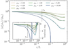Fig. 7. Scaling of $\langle {\varphi }_m^{+}{\varphi }_m\rangle$ for Δ = 1Δx (N = 10 0483) and ρth from 0.1 to 10.0. The inset shows the local scaling exponent ∂log(r)log$\langle {\varphi }_m^{+}{\varphi }_m\rangle$. The sonic scale rs is shown by the vertical black dotted line. The grey dashed line represents the fit using Eqs. (34) and (8).

Given that the set under consideration here is a surface-fractal, it is expected that the mass–size relation is M(r)∼r³. This appears in disagreement with the consensus based on robust numerical (Federrath et al. 2009; Kritsuk et al. 2007; Audit & Hennebelle 2010) and observational evidence in molecular clouds (see for instance the review by Roman-Duval et al. 2010; Hennebelle & Falgarone 2012, and references therein) for a mass fractal dimension D_m < 3. The origins for this disagreement are not yet clear. One first explanation is that the present method based on the correlation of the phase indicator field does not measure the same dimension as the one inferred by the methods of Kritsuk et al. (2007) and Federrath et al. (2009), which consists of measuring the mass contained in boxes of size r centred around the density peaks. Second, Kritsuk et al. (2007) and Federrath et al. (2009) use the original density field, while here we consider a thresholded version thereof. In other words, in the present framework, the mass can be viewed as being composed of a sum of weights, which are equal to either 0 or 1, while in Kritsuk et al. (2007) and Federrath et al. (2009), the mass is obtained after spatial integration of ρ over a box of size r. In Audit & Hennebelle (2010) the mass–size relationship is also inferred from a thresholded density field, but the mass is computed for each individual connected object and the scale is defined from the largest eigenvalue of the inertia tensor defined for each structure. These differences in the definition of both the mass and the scale are likely to explain the difference between our conclusion and the one reported by Audit & Hennebelle (2010).

4.3. Scale-space flux

The scale distribution of the flux ⟨(δu_∥)(δϕ)²⟩ for different values of the density threshold is shown in Fig. 8. We have chosen to normalise ⟨(δu_∥)(δϕ)²⟩ by 𝕂Σ. Using this normalisation, all curves collapse at small scales, which is in agreement with Eq. (27).

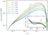Fig. 8. Scaling of ⟨(δu∥)(δϕ)2⟩ for ρth from 0.1 to 10.0. The inset shows the local scaling exponent. The horizontal dotted lines are the predicted scaling exponents ξu + ξs.

As a first remark, we note on Fig. 8 that ⟨(δu_∥)(δϕ)²⟩ is negative irrespective of the probed scale r. This means that the quantity ⟨(δϕ)²⟩ is transported towards smaller scales, following a direct cascade process. Hence, our results are consistent with the classical view that turbulence acts in stirring, stretching and folding the density field, thereby increasing its structural content. Broadly speaking, the turbulent velocity field acts in concentrating more interface into smaller volumes. The budget given by Eq. (26) then suggests that the velocity divergence counteracts this effect and is responsible for the expansion of density structures.

Second, we observe that although scaled in terms of strain rate, which for iso-density fields plays the same role as the scalar or the kinetic energy dissipation rate for the scalar variance or kinetic energy (Thiesset et al. 2020; Gauding et al. 2022), the flux depends quite significantly on the density threshold. This suggests that the dense, neutral and dilute regions do not equally interact with the turbulent velocity field. By contrast, the flux decreases with increasing ρ_th.

Thirdly, at intermediate scales, we observe the onset of a power-law behaviour for the flux term. This is better illustrated by the evolution of the local scaling exponent, shown in the inset of Fig. 8. A careful examination reveals that the scaling range is narrower than the one observed for ⟨(δϕ)²⟩ and appears at scales smaller than the sonic scale, which corresponds to the subsonic part of the turbulent spectrum. In this region of scales, Federrath et al. (2021) found that ⟨(δu_∥)²⟩^1/2 ∼ r^ξ_u where ξ_u = 0.39¹. As per Gauding et al. (2022), assuming that the flux scales as:

$$\begin{array}{c}\hfill ⟨(\delta u_{\Vert }){(\delta \varphi )}^2⟩\sim {⟨{(\delta u_{\Vert })}^2⟩}^{1/2}⟨{(\delta \varphi )}^2⟩,\end{array}$$(35)

we find that ⟨(δu_∥)(δϕ)²⟩ should scale as r^{ξ_u + ξ_s}. This prediction is plotted as the horizontal dotted lines in the inset of Fig. 8. Although not perfect, the agreement between this rather crude reasoning and numerical data is satisfactory. In particular, it reproduces rather well the decreasing evolution of the exponent for increasing ρ_th.

Finally, we note that similarly to the observations of Gauding et al. (2022) for iso-scalar surfaces in incompressible turbulence, there is not or only a very limited range of scales where the transfer rate is constant, that is where ⟨(δu_∥)(δϕ)²⟩∼r. The same observation was carried out by Ferrand et al. (2020) for the scale-by-scale transfer rate of kinetic energy. According to Ferrand et al. (2020), the non-constant energy transfer can be attributed to either shocks/discontinuities, yielding a loss of smoothness of the velocity field (Duchon & Robert 2000; Saw et al. 2016; Galtier 2018; Dubrulle 2019) or to non-local effects of the large-scale numerical forcing. We may also conjecture that the present numerical resolution, although unprecedented, is still not sufficient to observe a constant transfer of transported quantities (density, iso-density, or velocity) in the inertial range. This question is left unanswered.

4.4. Filtered quantities

We now proceed with the two-point statistical analysis of the phase indicator ϕ defined from filtered density $\overline{\rho }$ at varying filter size Δ and thresholded at a given ρ_th. For the sake of conciseness, we do not consider all above values for ρ_th, but focus on ρ_th = 1 only. Qualitatively similar observations were carried out for the other iso-density values.

The second-order structure function ⟨(δϕ)²⟩ for Δ/Δ_x varying from 1 to 32 is plotted in Fig. 9. As expected, increasing the filter size results in an earlier cutoff of ⟨(δϕ)²⟩ at small scales. The direct consequence is that the surface density Σ decreases with increasing Δ. More insights into this behaviour will be given in the next section, which focuses on the surface–size relation.

Fig. 9. Same as Fig. 6, but for ρth = 1.0 and Δ varying from 1 to 32Δx.

We note that the differences between the distributions for different Δ are rather small for Δ < 4Δ_x, but becomes significant for Δ ≥ 8Δ_x. However, the behaviour of ⟨(δϕ)²⟩ at large scales remains unaffected by the filter size, which indicates that (i) the measured volume fraction ⟨ϕ⟩, and (ii) the outer cutoff η_o do not depend on Δ. This may remain valid as long as Δ ≪ η_o. In Fig. 9, the fitted parametric expression given by Eq. (34) is plotted as the grey dashed lines. Here again, it shows that the proposed expression for ⟨(δϕ)²⟩ agrees very well with the numerical data. It can thus be used with confidence to unambiguously infer the geometric quantities Σ, η_o, η_i and ξ_s, even when the filter size is large, resulting in a restricted scaling range.

More insights can be provided by looking at the local scaling exponent of ⟨(δϕ)²⟩, which is shown in the inset of Fig. 9. It reveals that the extent of the power-law range becomes narrower with increasing Δ. The local scaling exponent appears to stabilise around a plateau at intermediate scales whose value depends on Δ. For the present ρ_th, the local scaling exponent obtained by fitting the numerical data using the parametric expression, Eq. (34), increases from about 0.46 for Δ = Δ_x to 0.52 for Δ = 32Δ_x. Therefore, these variations although measurable, are much smaller than the variations associated with different values of ρ_th (cf. Fig. 6). As a first approximation, one can thus assume that ξ_s depends only on the chosen iso-density, but remains constant, independently of the resolution Δ. Speculatively, the variation of ξ_s with Δ, though small, is evidence for a multi-fractal density field characterised by a fractal dimension that depends on the probed scale (Chappell & Scalo 2001). Here, it appears that when observed with a finer resolution, the fractal dimension is increasing, meaning that the interface is more tortuous, more space-filling. This statement about the multi-fractal character of iso-density sets, is rather hasty at this stage and a deeper analysis is required for being confirmed. This is left for future investigations.

The flux ⟨(δu_∥)(δϕ)²⟩ for varying filter size is presented in Fig. 10. Here again, we plot the results only for ρ_th = 1.0, but qualitatively similar conclusions were drawn for the other iso-density values. We again normalise the flux by 𝕂Σ, this quantity being estimated for Δ = 1Δ_x. Increasing the filter size Δ results again in a faster drop of the flux in the small-scale limit. This means that the measured strain rate 𝕂Σ decreases with increasing filter size. Comparing Figs. 10 and 9, we also note that the effect of Δ is somewhat more visible than it was for ⟨(δϕ)²⟩ and becomes substantial for Δ ≥ 2Δ_x. However, the distributions at large scales remain unchanged. The local scaling exponent for the flux ⟨(δu_∥)(δϕ)²⟩ (see the inset in Fig. 10) stabilises around a plateau whose value is only weakly affected by the filter size. As a result of a larger inner cut-off η_i, the extent of the scaling range diminishes measurably when Δ is increased.

Fig. 10. Same as Fig. 8, but for ρth = 1.0 and Δ varying from 1 to 32Δx.

In short, as long as η_i < Δ ≪ η_o, the large-scale distributions will not be affected by the filtering operation. In the opposite limit, that is for Δ ≪ η_i, both ⟨(δϕ)²⟩ and ⟨(δu_∥)(δϕ)²⟩ are independent of Δ over the entire range of scales. For η_i < Δ < η_o, the measured inner cutoff increases with Δ (more insights into this evolution is given in the next section), while the measured fractal dimension is only weakly affected by the filter size.

4.5. Surface-scale relation

For surface-fractals, the surface density Σ is expected to follow the relation (Sreenivasan et al. 1989):

$$\begin{array}{c}\hfill \mathrm{\Sigma }={\kappa }_{\mathrm{f}}{\left(\frac{{\eta }_{\mathrm{o}}}{{\eta }_{\mathrm{i}}}\right)}^{D_{\mathrm{s}}-2},\end{array}$$(36)

where κ_f is the fractal pre-factor, which has here the dimension of Σ (units of inverse length). It depends only on ρ_th but not on Δ. The quantities involved in Eq. (36) have been quantified by fitting the numerical estimations of ⟨(δϕ)²⟩ with the parametric expression of Eq. (34).

Let us first focus on the dependence of η_o with respect to Δ for different ρ_th. The latter is illustrated by triangles in Fig. 11. The limit of Eq. (34) when r → ∞, together with Eq. (23), reveals that

$$\begin{array}{c}\hfill 2⟨\varphi ⟩(1-⟨\varphi ⟩)=\frac{\mathrm{\Sigma }}{2}{\left(\frac{{\eta }_{\mathrm{o}}}{{\eta }_{\mathrm{i}}}\right)}^{2-D_{\mathrm{s}}}{\eta }_{\mathrm{o}}.\end{array}$$(37)

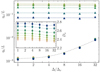Fig. 11. Inner cutoff ηi (circles) and outer cutoff ηo (triangles), together with the fractal dimension Ds (diamonds) as a function of Δ/Δx for different ρth ranging from 0.1 to 10.

By virtue of Eq. (36), we then have

$$\begin{array}{c}\hfill {\eta }_{\mathrm{o}}=4{\kappa }_f^{-1}⟨\varphi ⟩(1-⟨\varphi ⟩).\end{array}$$(38)

Thus, there exists a close link between the outer cutoff, the volume fraction and the fractal pre-factor. Since the measured volume fraction ⟨ϕ⟩ does not depend on Δ (see also Fig. 9), and that by definition, κ_f is function of ρ_th only, we thus predict that the outer cutoff η_o should be constant with respect to Δ. This prediction is confirmed by Fig. 11.

The fractal dimension D_s = 3 − ξ_s is displayed in the inset of Fig. 11 for the different filter sizes and different density iso-values investigated here. We note that, as observed previously for ρ_th = 1.0, the fractal dimension depends much more on ρ_th than on the filter size. Although small in amplitude, there seems to be increasing evolution of D_s when Δ decreases, before reaching an approximately constant value for Δ ≲ 4Δ_x. Overall, assuming that D_s is a function of ρ_th only, seems to be a reasonable assumption.

The evolution of the inner cutoff η_i for increasing filter size is also shown in Fig. 11. The first immediate conclusion is that η_i depends on Δ, but remains the same in dilute, dense, or neutral regions. Interestingly, Gauding et al. (2022) also found that η_i of passive scalar iso-surfaces in incompressible turbulence are independent of the iso-scalar value. These authors found that η_i can be predicted as the scale at which there is equilibrium between production (associated with the turbulent strain rate) and destruction of surface curvature (in their case related to scalar diffusion). The same reasoning applied to the present flow configuration suggests that the equilibrium between production and destruction of interface, associated here with turbulent straining and velocity divergence, respectively, is reached at the same scale irrespective of the probed iso-density value.

The second observation is that for small values of Δ, η_i is constant and starts increasing when Δ ≳ 4Δ_x. For large values of Δ, it is reasonable to assume that η_i ∼ Δ, while for any resolution Δ ≪ η_i, the interface tortuousness is fully resolved and the measured η_i is constant and is equal to ${\eta }_{\mathrm{i}}^u$: the unfiltered inner cutoff. These two distinct behaviours:

$$\begin{array}{c}\hfill {\eta }_{\mathrm{i}}(\mathrm{\Delta })\{\begin{array}{c}={\eta }_{\mathrm{i}}^u\mathrm{if}\mathrm{\Delta }\ll {\eta }_{\mathrm{i}}^u\hfill \\ \sim \mathrm{\Delta }\mathrm{if}\mathrm{\Delta }\gg {\eta }_{\mathrm{i}}^u,\hfill \end{array}\end{array}$$(39)

can be combined into a single expression of the form

$$\begin{array}{c}\hfill {\eta }_{\mathrm{i}}(\mathrm{\Delta })={\eta }_{\mathrm{i}}^u{[1+{\left(\frac{a\mathrm{\Delta }}{{\eta }_{\mathrm{i}}^u}\right)}^b]}^{1/b},\end{array}$$(40)

where a and b are two constants of order unity. In Fig. 11, Eq. (40) is compared to the numerical data. We find that a = 1.25 and b = 2 provide satisfactory results, although we did not seek for the most suitable values (we did not perform any least-square fit). The unfiltered inner cutoff ${\eta }_{\text{i}}^u$ is found to be ${\eta }_{\text{i}}^u=(1.26\pm 0.04)\times {10}^{-3}L\approx 6{\mathrm{\Delta }}_x$. It is worth stressing that here, the inner cutoff is set artificially by numerical dissipation. In reality, the inner cutoff scale may be of the same order as the viscous scales (Gauding et al. 2022).

In Fig. 12, we plot the specific surface density Σ_s, defined as the ratio between the surface area of the interface and the volume of the minority phase. The specific surface density is thus related to the above defined surface density Σ by Σ_s = Σ/⟨ϕ_m⟩=Σ/min(⟨ϕ⟩,1 − ⟨ϕ⟩). The values for Σ_s are computed from the fitted parametric expression, Eq. (34), and are represented with the circle symbols in Fig. 12. A first observation is that the specific surface for the dense regions is much higher than that of the neutral or dilute regions. In other words, dense regions are the ones for which the ratio between the surface area and the volume is the highest. This is consistent with our previous conclusions that the surface fractal dimension D_s is larger for high density regions, meaning that the interface is more corrugated.

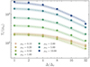Fig. 12. Specific surface Σ/⟨ϕm⟩ as a function of Δ/Δx for ρth ranging from 0.1 to 10. The dashed lines show the prediction with Σ = κf(ηo/ηi)Ds − 2. The coloured filled regions correspond to a relative error of ±10%.

The evolution of Σ_s with respect to the filter size is qualitatively similar irrespective of the iso-density. For small values of the filter size, for $\mathrm{\Delta }<{\eta }_{\text{i}}^u$, it reaches a constant value and decreases for any filter size $\mathrm{\Delta }>{\eta }_{\text{i}}^u$. For large values of Δ, we observe the onset of a power law for the specific surface density with respect to Δ. The evolution of the filtered specific surface density can be well predicted by the surface-fractal model. Indeed, using Eq. (38) to express the fractal pre-factor κ_f in terms of ⟨ϕ⟩ and η_o, we end up with the following expression for Σ_s:

$$\begin{array}{c}\hfill {\mathrm{\Sigma }}_{\mathrm{s}}=4\frac{⟨\varphi ⟩(1-⟨\varphi ⟩)}{{\eta }_{\mathrm{o}}⟨{\varphi }_m⟩}{\left(\frac{{\eta }_{\mathrm{o}}}{{\eta }_{\mathrm{i}}}\right)}^{D_{\mathrm{s}}-2}.\end{array}$$(41)

This expression is tested in Fig. 12. Predictions are illustrated using the dashed lines, where η_o, η_i and D_s were also extracted from the fitting procedure. We note a close agreement irrespective of the iso-density value. Some discrepancies between the model and the numerical data are in the range ±10%, which is illustrated by the coloured filled regions. The adequacy of Eq. (41) is further evidence that the iso-density sets are surface-fractals.

The power-law behaviour for Σ_s at large Δ can be derived. For this purpose, one needs (i) to recall that η_o and ⟨ϕ⟩ depend only on ρ_th, while (ii) η_i is proportional to Δ in the limit of large Δ, and finally (iii) assume that D_s is constant with respect to Δ. With this, we obtain that Σ_s ∼ Δ^{2 − D_s}, which is the known surface–size relation for surface fractals. This simple expression (and the more detailed one given by Eq. (41)) can be readily used to compare the iso-density surface area estimated using different numerical and/or observational resolutions at the condition that D_s is known. Equation (41) also requires the parameter ${\eta }_{\text{i}}^u$ to be known. Conversely, this relation can also be used to estimate the surface fractal dimension and the inner cutoff, using numerical and/or observational data filtered at different resolutions.

In case of observational data, since we dispose only of integrated visualisations, a hypothesis is required for the third dimension. One could for example assume fractal isotropy and then look at the perimeter of the iso-line formed by a given iso-value (as was done for instance by Federrath et al. 2009), replacing the exponent by 1 − D_s in Eq. (41) (see also work by Sánchez et al. 2005; Beattie et al. 2019a,b). Therefore, this fractal surface-size relation could help in providing insights into the structural content of the density field inferred from either numerical simulations or observations. This question could be addressed in a follow-up study.

4.6. Relation to the virial theorem

Following Ballesteros-Paredes et al. (1999) and Dib et al. (2007), let the virial theorem be applied to a volume V_ρ enclosed by the iso-surface ρ(x, t) = ρ_th. The volume boundary is denoted ∂V_ρ. The Lagrangian formulation for the virial theorem can be written in symbolic form (Chandrasekhar & Fermi 1953; McKee & Zweibel 1992; Ballesteros-Paredes 2006) as

$$\begin{array}{c}\hfill \frac{1}{2}{\ddot{I}}_L=2({\mathcal{E}}_{\mathrm{kin}}+{\mathcal{E}}_{\mathrm{int}})+{\mathcal{E}}_{\mathrm{mag}}-2{\mathcal{T}}_{\mathrm{int}}-{\mathcal{T}}_{\mathrm{mag}}-\mathcal{W},\end{array}$$(42)

where I_L is the moment of inertia of the volume under consideration. The terms denoted with the letter ℰ in Eq. (42) are the volume integrals of the kinetic, internal and magnetic energy density, respectively, given by

$$\begin{array}{cc}& {\mathcal{E}}_{\mathrm{kin}}=\frac{1}{2}{\displaystyle {\int }_{V_{\rho }}\rho u^2\mathrm{d}V,}\hfill \end{array}$$(43a)

$$\begin{array}{cc}& {\mathcal{E}}_{\mathrm{int}}=\frac{3}{2}{\displaystyle {\int }_{V_{\rho }}p\mathrm{d}V,}\hfill \end{array}$$(43b)

$$\begin{array}{cc}& {\mathcal{E}}_{\mathrm{mag}}=\frac{1}{8\pi }{\displaystyle {\int }_{V_{\rho }}{B}^2\mathrm{d}V.}\hfill \end{array}$$(43c)

The terms denoted with the letter 𝒯 are surface integrals:

$$\begin{array}{cc}& {\mathcal{T}}_{\mathrm{int}}=\frac{1}{2}{\displaystyle {\int }_{\partial V_{\rho }}p\mathit{x}·\mathit{n}\mathrm{d}S,}\hfill \end{array}$$(44a)

$$\begin{array}{cc}& {\mathcal{T}}_{\mathrm{mag}}=\frac{1}{4\pi }{\displaystyle {\int }_{\partial V_{\rho }}\mathcal{B}\mathrm{d}S,}\hfill \end{array}$$(44b)

and represents the surface integrated pressure and magnetic stresses, respectively. The quantity ℬ is given by:

$$\begin{array}{c}\hfill \mathcal{B}=\mathit{x}·(\mathit{B}\mathit{B}-\frac{1}{2}{B}^2\mathit{I})·\mathit{n}.\end{array}$$(45)

The last term in Eq. (42) represents the effect of gravity and reads:

$$\begin{array}{c}\hfill {\mathcal{W}}_{\mathrm{int}}={\displaystyle {\int }_{V_{\rho }}\mathit{x}·\mathbf{\nabla }\mathrm{\Psi }\mathrm{d}V,}\end{array}$$(46)

where Ψ is the gravitational potential. In previous equations, positions and velocity are defined relative to the positions and velocity of the centre of mass. Dividing all terms in Eq. (42) by V_ρ = ⟨ϕ⟩V, the three volume integrals in Eq. (42) can be rewritten as:

$$\begin{array}{cc}& \frac{1}{⟨\varphi ⟩V}(2{\mathcal{E}}_{\mathrm{kin}}+2{\mathcal{E}}_{\mathrm{int}}+{\mathcal{E}}_{\mathrm{mag}}-\mathcal{W})=\hfill \\ \hfill & {⟨\rho u^2⟩}_{\rho }+3{⟨p⟩}_{\rho }+\frac{1}{8\pi }{⟨B^2⟩}_{\rho }+{⟨\mathit{x}·\mathbf{\nabla }\mathrm{\Psi }⟩}_{\rho },\hfill \end{array}$$(47)

where the brackets ⟨ • ⟩_ρ stand for a volume average over V_ρ:

$$\begin{array}{c}\hfill {⟨\bullet ⟩}_{\rho }=\frac{1}{V_{\rho }}{\displaystyle {\int }_{V_{\rho }}\bullet \mathrm{d}V=\frac{1}{⟨\varphi ⟩V}{\int }_{V_{\rho }}\bullet \mathrm{d}V.}\end{array}$$(48)

Similarly, it is convenient to use the surface area weighted average:

$$\begin{array}{c}\hfill {⟨\bullet ⟩}_{\mathrm{s}}=\frac{1}{S}{\displaystyle {\int }_{\partial V_{\rho }}\bullet \mathrm{d}S=\frac{1}{\mathrm{\Sigma }V}{\int }_{\partial V_{\rho }}\bullet \mathrm{d}S,}\end{array}$$(49)

which allows the surface integrals to be rewritten as

$$\begin{array}{c}\hfill \frac{1}{⟨\varphi ⟩V}(2{\mathcal{T}}_{\mathrm{int}}+{\mathcal{T}}_{\mathrm{mag}})=\frac{1}{⟨\varphi ⟩}[{⟨p\mathit{x}·\mathit{n}⟩}_{\mathrm{s}}+\frac{1}{4\pi }{⟨\mathcal{B}⟩}_{\mathrm{s}}]\mathrm{\Sigma }.\end{array}$$(50)

Finally, the virial theorem can be recast in the form

$$\begin{array}{cc}\hfill \frac{1}{2V}{\ddot{I}}_L& =[{⟨\rho u^2⟩}_{\rho }+3{⟨p⟩}_{\rho }+\frac{1}{8\pi }{⟨B^2⟩}_{\rho }+{⟨\mathit{x}·\mathbf{\nabla }\mathrm{\Psi }⟩}_{\rho }]⟨\varphi ⟩\hfill \\ \hfill & -[{\langle p\mathit{x}·\mathit{n}\rangle }_{\mathrm{s}}+\frac{1}{4\pi }{\langle \mathcal{B}\rangle }_{\mathrm{s}}]\mathrm{\Sigma }.\hfill \end{array}$$(51)

As before, V_ρ/V = ⟨ϕ⟩ is the volume occupied by the volume enclosed by the surface ρ(x, t) = ρ_th divided by V (the observed volume), and Σ = S/V is the surface density of this surface. A similar expression for the virial theorem in the Eulerian form (McKee & Zweibel 1992) can de derived.

The merit of formulating the virial theorem in the form proposed here is that it draws connections between the geometry of the density field (⟨ϕ⟩ and Σ) and its dynamics (the terms within the brackets). It further allows the gravitational equilibrium to be probed for each iso-density value separately. The different terms in Eq. (51) cannot be inferred from observations without invoking some simplifying assumptions. They can, however, be estimated from numerical simulations (Ballesteros-Paredes et al. 1999; Dib et al. 2007), thereby opening interesting perspectives to explore the relation between the geometry and the dynamics of the ISM.

5. Conclusion

The present work aims at exploring the role of supersonic turbulence in shaping the microstructure of the density field. For this purpose, we propose using a two-point statistical analysis of the phase indicator field ϕ defined by iso-density sets, Eq. (1). The asymptotic behaviour for the correlation and structure functions of iso-sets, at small, intermediate and large-scales, are derived theoretically and discussed. These relations revealed that the two-point statistics of ϕ depend on some geometric features such as the volume-fraction, the surface density, the curvature, and the fractal characteristics of the gas density field. It is also shown that comparing the correlation and structure function at intermediate scales, allows one to assess whether the medium under consideration is a mass-fractal or a surface-fractal, with important consequences for the mass–size relation. We also derive the transport equation for the correlation and structure functions, emphasising the role of velocity and velocity dilatation in the structural evolution of the density field.

This framework is here appraised using data from highly resolved numerical simulations of supersonic isothermal turbulence. We consider both the original dataset together with the associated filtered quantities in order to establish the surface–size relation of the iso-density fields.

Our results indicate that iso-density sets of supersonic isothermal turbulence are surface-fractals rather than mass-fractals, except maybe for the very dense regions. The surface-fractal dimension D_s depends significantly on the iso-density value, and increases with increasing density threshold ρ_th. The consequence is that the specific surface density is higher in the dense regions compared to the dilute or neutral regions. The surface-fractal dimension varies only slightly with the filter size. As a first approximation, it is thus reasonable to assume that D_s depends only on ρ_th. A direct consequence of the surface fractality of iso-density fields is a model to predict the surface density as a function of the resolution scale. This model could be used to assess the surface-fractal dimension D_s from observations and numerical simulations of the interstellar medium.

The transport equation for the correlation and structure functions reveals that the turbulent cascade and dilatation are two competing effects. The numerical simulation data indicate that the flux in the cascade is negative, meaning that the transfer is occurring from large to small scales (direct cascade). In other words, irrespectively of the probed scale, turbulence acts in concentrating more interface into smaller volumes. Here, dilatation compensates turbulent straining, such that a steady state can be reached. A local scaling range is observed for the flux of iso-density in scale-space, with an exponent that appears to depend on both the velocity and the iso-density power-law scaling. In agreement with Ferrand et al. (2020) for the cascade of kinetic energy, we do not find a clear range of scales complying with a constant scale-transfer (linear flux). As anticipated by Ferrand et al. (2020), the loss of smoothness of the velocity field and non-local effects of the velocity forcing could explain this observation. We may also conjecture that, though already fine, the resolution is still not fine enough to observe a clear separation of scales between the forcing at large scales and numerical dissipation at small scales, for the phase indicator field ϕ.

Finally, a formulation for the virial theorem in terms of ϕ is developed, which makes explicit the relation between the geometry of the density field (the volume and surface density) and its dynamics. This new formulation together with the proposed framework based on the two-point statistics of the phase indicator may offer interesting perspectives to better understand the dynamics of the ISM.

Acknowledgments

FT acknowledges A. Poux and M. Gauding for their help in the development of the post-processing routines. We thank J. Yon from the CORIA laboratory for providing the illustration of a soot particle shown in Fig. 1. CF acknowledges funding provided by the Australian Research Council (Future Fellowship FT180100495 and Discovery Projects DP230102280), and the Australia-Germany Joint Research Cooperation Scheme (UA-DAAD). We acknowledge computational time granted by the CRIANN (project 2018002), by the Jülich Supercomputing Centre (project instahype). We further acknowledge high-performance computing resources provided by the Australian National Computational Infrastructure (grant ek9) and the Pawsey Supercomputing Centre (project pawsey0810) in the framework of the National Computational Merit Allocation Scheme and the ANU Merit Allocation Scheme, and by the Leibniz Rechenzentrum and the Gauss Centre for Supercomputing (grants pr32lo, pr48pi, pn73fi, and GCS Large-scale projects 10391 and 22542). The simulation software FLASH was in part developed by the DOE-supported Flash Center for Computational Science at the University of Chicago.

References

Appendix A: Simulations at different resolutions

In addition to analysing data at different filter size Δ_x, we computed the same quantities as in Figs. 11 and 12 using different simulations at different resolutions Δ_x. These simulations were performed using different grid size of 10048³, 5024³, 2512³, 1256³ and 628³ grid points, respectively.

The evolution of the inner and outer cutoff together with the fractal dimension for different resolution Δ_x are presented in Fig. A.1. We observe again that the fractal dimension D_s depends mainly on the iso-density threshold, while the influence of Δ_x is weaker, though measurable. The inner cutoff η_i appears linear throughout the range of Δ_x. This means that the cutoff is set by numerical dissipation which increases with Δ_x. Finally, and the most surprising is that the outer cutoff η_o which was found to be constant with respect to the filter size now slightly increases with the grid size. We do not have yet an explanation for this, but we note however that the increase is quite weak.

Fig. A.1. Same as Fig. 11, but using data from different simulations at different resolutions Δx

With these values for η_o, η_i and D_s, the surface density Σ_s can be predicted and compared to the one actually computed. Results are shown in Fig. A.2. It reveals that the surface-fractal model applies nicely with departures that are within 10%. The overall conlusion is that, with all other parameters kept unchanged, carrying out a simulation at a given resolution Δ_x is not equivalent to coarse-graining the finer simulation using a filter size Δ_x.

Fig. A.2. Same as Fig. 12, but using data from different simulations at different resolutions Δx

All Figures

	Fig. 1. Illustrations of different categories of fractals. Examples of mass-fractals: (a) a soot particle and (c) the Menger sponge. Examples of surface-fractals : (b) a coastline and (d) the Julia set.
In the text

	Fig. 2. Correlation and structure function for the Menger sponge and the axisymmetric Julia set (z ⇌ z2 − 1). The grey dotted line represents the theoretical power laws with Dm = log3(20) for the Menger sponge and Ds ≈ 2.27 for the Julia set.
In the text

	Fig. 3. Schematic representation of the different asymptotic regimes of ⟨(δϕ)2⟩ and $\langle {\varphi }_m^{+}{\varphi }_m\rangle$ for different scale ranges from small to large scales.
In the text

	Fig. 4. Two-dimensional slices of the density field and their associated phase indicator field. (a) slice of log(ρ/ρ0) with light (dark) colours corresponding to low (high) values. (b–h) Corresponding iso-density set with ρth = 0.1 to 10.0, as indicated in the legend of each panel. The yellow and blue regions correspond to ϕ = 0 and ϕ = 1, respectively.
In the text

	Fig. 5. Volume fraction ⟨ϕ⟩ for the different values of ρth (symbols). The black solid line corresponds to the prediction of Eq. (33) with a dispersion parameter σs = 1.21.
In the text

	Fig. 6. Scaling of ⟨(δϕ)2⟩ for Δ = 1Δx, that is N = 10 0483 and ρth from 0.1 to 10.0. The inset shows the local scaling exponent ∂log(r)log⟨(δϕ)2⟩. The grey dashed line represents the fit using Eq. (34). The sonic scale rs is shown by the vertical black dotted line.
In the text

	Fig. 7. Scaling of $\langle {\varphi }_m^{+}{\varphi }_m\rangle$ for Δ = 1Δx (N = 10 0483) and ρth from 0.1 to 10.0. The inset shows the local scaling exponent ∂log(r)log$\langle {\varphi }_m^{+}{\varphi }_m\rangle$. The sonic scale rs is shown by the vertical black dotted line. The grey dashed line represents the fit using Eqs. (34) and (8).
In the text

	Fig. 8. Scaling of ⟨(δu∥)(δϕ)2⟩ for ρth from 0.1 to 10.0. The inset shows the local scaling exponent. The horizontal dotted lines are the predicted scaling exponents ξu + ξs.
In the text

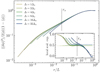	Fig. 9. Same as Fig. 6, but for ρth = 1.0 and Δ varying from 1 to 32Δx.
In the text

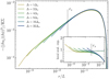	Fig. 10. Same as Fig. 8, but for ρth = 1.0 and Δ varying from 1 to 32Δx.
In the text

	Fig. 11. Inner cutoff ηi (circles) and outer cutoff ηo (triangles), together with the fractal dimension Ds (diamonds) as a function of Δ/Δx for different ρth ranging from 0.1 to 10.
In the text

	Fig. 12. Specific surface Σ/⟨ϕm⟩ as a function of Δ/Δx for ρth ranging from 0.1 to 10. The dashed lines show the prediction with Σ = κf(ηo/ηi)Ds − 2. The coloured filled regions correspond to a relative error of ±10%.
In the text

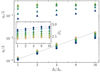	Fig. A.1. Same as Fig. 11, but using data from different simulations at different resolutions Δx
In the text

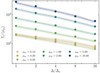	Fig. A.2. Same as Fig. 12, but using data from different simulations at different resolutions Δx
In the text

References

- Adler, P. M., Jacquin, C. G., & Quiblier, J. A. 1990, Int. J. Multiphase Flow, 16, 691 [CrossRef] [Google Scholar]
- Aluie, H. 2013, Phys. D: Nonl. Phenom., 247, 54 [NASA ADS] [CrossRef] [Google Scholar]
- Appel, S. M., Burkhart, B., Semenov, V. A., Federrath, C., & Rosen, A. L. 2022, ApJ, 927, 75 [NASA ADS] [CrossRef] [Google Scholar]
- Audit, E., & Hennebelle, P. 2010, A&A, 511, A76 [NASA ADS] [CrossRef] [EDP Sciences] [Google Scholar]
- Ballesteros-Paredes, J. 2006, MNRAS, 372, 443 [NASA ADS] [CrossRef] [Google Scholar]
- Ballesteros-Paredes, J., Vázquez-Semadeni, E., & Scalo, J. 1999, ApJ, 515, 286 [CrossRef] [Google Scholar]
- Beattie, J. R., Federrath, C., & Klessen, R. S. 2019a, MNRAS, 487, 2070 [NASA ADS] [CrossRef] [Google Scholar]
- Beattie, J. R., Federrath, C., Klessen, R. S., & Schneider, N. 2019b, MNRAS, 488, 2493 [NASA ADS] [CrossRef] [Google Scholar]
- Berryman, J. G. 1987, J. Math. Phys., 28, 244 [NASA ADS] [CrossRef] [Google Scholar]
- Burkhart, B., & Mocz, P. 2019, ApJ, 879, 129 [NASA ADS] [CrossRef] [Google Scholar]
- Candel, S., & Poinsot, T. 1990, Combust. Sci. Technol., 70, 1 [CrossRef] [Google Scholar]
- Chandrasekhar, S., & Fermi, E. 1953, ApJ, 118, 116 [Google Scholar]
- Chappell, D., & Scalo, J. 2001, ApJ, 551, 712 [Google Scholar]
- Ciccariello, S. 1995, J. Math. Phys., 36, 219 [NASA ADS] [CrossRef] [Google Scholar]
- Danaila, L., Antonia, R. A., & Burattini, P. 2004, New J. Phys., 6, 128 [NASA ADS] [CrossRef] [Google Scholar]
- de Silva, C. M., Philip, J., Chauhan, K., Meneveau, C., & Marusic, I. 2013, Phys. Rev. Lett., 111, 044501 [NASA ADS] [CrossRef] [Google Scholar]
- Debye, P., Anderson, H. R., Jr, & Brumberger, H. 1957, J Appl. Phys., 28, 679 [NASA ADS] [CrossRef] [Google Scholar]
- Dib, S., Kim, J., Vázquez-Semadeni, E., Burkert, A., & Shadmehri, M. 2007, ApJ, 661, 262 [NASA ADS] [CrossRef] [Google Scholar]
- Dubey, A., Fisher, R., Graziani, C., et al. 2008, ASP Conf. Ser., 385, 145 [NASA ADS] [Google Scholar]
- Dubrulle, B. 2019, J. Fluid Mech., 867, P1 [NASA ADS] [CrossRef] [Google Scholar]
- Duchon, J., & Robert, R. 2000, Nonlinearity, 13, 249 [CrossRef] [MathSciNet] [Google Scholar]
- Elmegreen, B. G., & Falgarone, E. 1996, ApJ, 471, 816 [NASA ADS] [CrossRef] [Google Scholar]
- Elmegreen, B. G., & Scalo, J. 2004, ARA&A, 42, 211 [Google Scholar]
- Elsas, J. H., Szalay, A. S., & Meneveau, C. 2018, J. Turbul., 19, 297 [NASA ADS] [CrossRef] [Google Scholar]
- Federrath, C. 2015, MNRAS, 450, 4035 [Google Scholar]
- Federrath, C., & Klessen, R. S. 2012, ApJ, 761, 156 [Google Scholar]
- Federrath, C., & Klessen, R. S. 2013, ApJ, 763, 51 [Google Scholar]
- Federrath, C., Klessen, R. S., & Schmidt, W. 2008, ApJ, 688, L79 [NASA ADS] [CrossRef] [Google Scholar]
- Federrath, C., Klessen, R. S., & Schmidt, W. 2009, ApJ, 692, 364 [Google Scholar]
- Federrath, C., Roman-Duval, J., Klessen, R., Schmidt, W., & Mac Low, M.-M. 2010, A&A, 512, A81 [NASA ADS] [CrossRef] [EDP Sciences] [Google Scholar]
- Federrath, C., Klessen, R. S., Iapichino, L., & Beattie, J. R. 2021, Nat. Astron., 5, 365 [NASA ADS] [CrossRef] [Google Scholar]
- Federrath, C., Roman-Duval, J., Klessen, R. S., Schmidt, W., & Mac Low, M. M. 2022, Astrophysics Source Code Library [record ascl:2204.001] [Google Scholar]
- Ferrand, R., Galtier, S., Sahraoui, F., & Federrath, C. 2020, ApJ, 904, 160 [NASA ADS] [CrossRef] [Google Scholar]
- Frisch, H. L., & Stillinger, F. H. 1963, J. Chem. Phys., 38, 2200 [NASA ADS] [CrossRef] [Google Scholar]
- Fryxell, B., Olson, K., Ricker, P., et al. 2000, ApJS, 131, 273 [Google Scholar]
- Galtier, S. 2018, J. Phys. A: Math. Theor., 51, 205501 [NASA ADS] [CrossRef] [Google Scholar]
- Galtier, S., & Banerjee, S. 2011, Phys. Rev. Lett., 107, 134501 [NASA ADS] [CrossRef] [Google Scholar]
- Gauding, M., Thiesset, F., Varea, E., & Danaila, L. 2022, J. Fluid Mech., 942, A14 [NASA ADS] [CrossRef] [Google Scholar]
- Girichidis, P., Konstandin, L., Whitworth, A. P., & Klessen, R. S. 2014, ApJ, 781, 91 [CrossRef] [Google Scholar]
- Guinier, A., Fournet, G., & Yudowitch, K. L. 1955, Small-angle Scattering of X-rays (New York: Wiley) [Google Scholar]
- Hawkes, E. R., Chatakonda, O., Kolla, H., Kerstein, A. R., & Chen, J. H. 2012, Combustion and Flame, 159, 2690 [CrossRef] [Google Scholar]
- Hennebelle, P., & Chabrier, G. 2008, ApJ, 684, 395 [Google Scholar]
- Hennebelle, P., & Falgarone, E. 2012, A&ARv, 20, 1 [CrossRef] [Google Scholar]
- Hentschel, H. G. E., & Procaccia, I. 1984, Phys. Rev. A, 29, 1461 [NASA ADS] [CrossRef] [Google Scholar]
- Heyer, M. H., & Brunt, C. M. 2004, ApJ, 615, L45 [NASA ADS] [CrossRef] [Google Scholar]
- Hopkins, P. F. 2013, MNRAS, 430, 1880 [Google Scholar]
- Kainulainen, J., Federrath, C., & Henning, T. 2014, Science, 344, 183 [NASA ADS] [CrossRef] [Google Scholar]
- Khullar, S., Federrath, C., Krumholz, M. R., & Matzner, C. D. 2021, MNRAS, 507, 4335 [NASA ADS] [CrossRef] [Google Scholar]
- Kim, J., & Ryu, D. 2005, ApJ, 630, L45 [NASA ADS] [CrossRef] [Google Scholar]
- Kirste, R., & Porod, G. 1962, Kolloid-Zeitschrift und Zeitschrift für Polymere, 184, 1 [CrossRef] [Google Scholar]
- Kolmogorov, A. 1941, Dokl. Akad. Nauk. SSSR, 125, 15 [Google Scholar]
- Kritsuk, A. G., Norman, M. L., & Padoan, P. 2006, ApJ, 638, L25 [NASA ADS] [CrossRef] [Google Scholar]
- Kritsuk, A. G., Norman, M. L., Padoan, P., & Wagner, R. 2007, ApJ, 665, 416 [NASA ADS] [CrossRef] [Google Scholar]
- Kritsuk, A. G., Norman, M. L., & Wagner, R. 2011, ApJ, 727, L20 [NASA ADS] [CrossRef] [Google Scholar]
- Krug, D., Holzner, M., Marusic, I., & van Reeuwijk, M. 2017, J. Fluid Mech., 820, R3 [NASA ADS] [CrossRef] [Google Scholar]
- Krumholz, M. R., & McKee, C. F. 2005, ApJ, 630, 250 [Google Scholar]
- Krumholz, M. R., Klein, R. I., & McKee, C. F. 2012, ApJ, 754, 71 [NASA ADS] [CrossRef] [Google Scholar]
- Lu, J., & Tryggvason, G. 2018, Phys. Rev. Fluids, 3, 084401 [NASA ADS] [CrossRef] [Google Scholar]
- Lu, J., & Tryggvason, G. 2019, Phys. Rev. Fluids, 4, 084301 [NASA ADS] [CrossRef] [Google Scholar]
- Mac Low, M.-M., & Klessen, R. S. 2004, Rev. Modern Phys., 76, 125 [NASA ADS] [CrossRef] [Google Scholar]
- McKee, C. F., & Ostriker, E. C. 2007, ARA&A, 45, 565 [Google Scholar]
- McKee, C. F., & Zweibel, E. G. 1992, ApJ, 399, 551 [CrossRef] [Google Scholar]
- Morán, J., Fuentes, A., Liu, F., & Yon, J. 2019, Comput. Phys. Commun., 239, 225 [CrossRef] [Google Scholar]
- Myers, A. T., Klein, R. I., Krumholz, M. R., & McKee, C. F. 2014, MNRAS, 439, 3420 [NASA ADS] [CrossRef] [Google Scholar]
- Ossenkopf, V., & Mac Low, M.-M. 2002, A&A, 390, 307 [NASA ADS] [CrossRef] [EDP Sciences] [Google Scholar]
- Padoan, P., & Nordlund, Å. 2002, ApJ, 576, 870 [NASA ADS] [CrossRef] [Google Scholar]
- Padoan, P., & Nordlund, Å. 2011, ApJ, 730, 40 [Google Scholar]
- Padoan, P., Jimenez, R., Juvela, M., & Nordlund, Å. 2004, ApJ, 604, L49 [NASA ADS] [CrossRef] [Google Scholar]
- Padoan, P., Federrath, C., Chabrier, G., et al. 2014, in Protostars and Planets VI, eds. H. Beuther, R. S. Klessen, C. P. Dullemond, & T. Henning (University of Arizona Press), 77 [Google Scholar]
- Passot, T., & Vázquez-Semadeni, E. 1998, Phys. Rev. E, 58, 4501 [Google Scholar]
- Porod, G. 1951, Kolloid-Zeitschrift, 124, 83 [CrossRef] [Google Scholar]
- Roman-Duval, J., Jackson, J. M., Heyer, M., Rathborne, J., & Simon, R. 2010, ApJ, 723, 492 [NASA ADS] [CrossRef] [Google Scholar]
- Sánchez, N., Alfaro, E. J., & Pérez, E. 2005, ApJ, 625, 849 [CrossRef] [Google Scholar]
- Saw, E.-W., Kuzzay, D., Faranda, D., et al. 2016, Nat. Commun., 7, 12466 [NASA ADS] [CrossRef] [Google Scholar]
- Schneider, N., Bontemps, S., Motte, F., et al. 2016, A&A, 587, A74 [NASA ADS] [CrossRef] [EDP Sciences] [Google Scholar]
- Sorensen, C. M. 2001, Aerosol Sci. Technol., 35, 648 [NASA ADS] [CrossRef] [Google Scholar]
- Sreenivasan, K. R., Ramshankar, R., & Meneveau, C. 1989, Proc. R. Soc. London. A. Math. Phys. Sci., 421, 79 [Google Scholar]
- Stutzki, J., Bensch, F., Heithausen, A., Ossenkopf, V., & Zielinsky, M. 1998, A&A, 336, 697 [NASA ADS] [Google Scholar]
- Teubner, M. 1990, J. Chem. Phys., 92, 4501 [NASA ADS] [CrossRef] [Google Scholar]
- Thiesset, F., & Poux, A. 2020, Numerical Assessment of the Two-point Statistical Equations in Liquid/gas Flows, Tech. rep., CNRS, Normandy Univ., UNIROUEN, INSA Rouen, CORIA [Google Scholar]
- Thiesset, F., Maurice, G., Halter, F., et al. 2016, Phys. Rev. E, 93, 013116 [NASA ADS] [CrossRef] [Google Scholar]
- Thiesset, F., Duret, B., Ménard, T., et al. 2020, J. Fluid Mech., 886, A4 [NASA ADS] [CrossRef] [Google Scholar]
- Thiesset, F., Ménard, T., & Dumouchel, C. 2021, J. Fluid Mech., 912, A39 [NASA ADS] [CrossRef] [Google Scholar]
- Torquato, S. 2002, Random Heterogeneous Materials. Microstructure and Macroscopic Properties (New York: Springer-Verlag) [CrossRef] [Google Scholar]
- Vassilicos, J. C. 1992, Topological aspects of the dynamics of fluids and plasmas, eds. H. K. Moffatt, G. M. Zaslavsky, P. Comte, & M. Tabor (Springer), 427 [CrossRef] [Google Scholar]
- Vassilicos, J. C., & Hunt, J. C. R. 1991, Proc. R. Soc. London. Ser. A: Math. Phys. Sci., 435, 505 [Google Scholar]
- Vassilicos, J. C., & Hunt, J. C. R. 1996, Institute of Mathematics and its Applications Conference Series (Oxford University Press), 56, 127 [Google Scholar]
- Vazquez-Semadeni, E. 1994, ApJ, 423, 681 [Google Scholar]
- Waagan, K., Federrath, C., & Klingenberg, C. 2011, J. Comput. Phys., 230, 3331 [NASA ADS] [CrossRef] [Google Scholar]
- Wong, P.-Z., & Cao, Q.-Z. 1992, Phys. Rev. B, 45, 7627 [NASA ADS] [CrossRef] [Google Scholar]
- Yaglom, A. 1949, Dokl. Akad. Nauk. SSSR, 69, 743 [Google Scholar]