© P. Tremblin et al. 2022

1. Introduction

Astrophysical flows are by nature multiscale systems exhibiting a wide range of dynamical regimes that is remains quite challenging to understand. Since the 1970s and 1980s, hydro- or N-body high- performance numerical simulations have been key tools for understanding self-gravitating systems. However, a proper understanding of collective effects in these simulations remains challenging, notably because of numerical artifacts. Therefore, theory remains vital to assess the genuine validity of the numerical simulations.

The theoretical description of an ensemble of particles is a challenging task that has motivated the development of a major domain in physics: statistical mechanics. The statistical descriptions of a gas and a solid are relatively easy in two limiting cases: perfect disorder, often referred to as molecular chaos for ideal gases, or perfect order for ordered solids. The description of liquids, or ill-condensed systems, however, is much more complex and has only been possible after the pioneering work of Bogolyubov, Born, Green, Kirkwood, and Yvon, referred to as the BBGKY hierarchy (e.g., Yvon 1935; Born & Green 1946; Bogoliubov 1946; Kirkwood 1946). Within this framework, the ensemble of particles is described by the one-particle probability density function, the two-particle probability density function, and so on. Truncated at the second order, the system is described by the one-particle density function and the pair correlation function, generally referred to as the radial distribution function in liquid statistical mechanics. In the case of perfect chaos for an ideal gas, the radial distribution function is uniformly equal to 1, which means that there is no correlation in the fluid: the probability of finding two particles at two given points is equal to the product of the probabilities of finding one particle at these given points.

Liquids differ from an ideal gas because of the presence of interparticle forces that lead to correlations at short distances, and they differ from solids because of the lack of (periodic) long-range order (i.e., the pair correlation function tends to 1 at long distance). For water, the dominant effects responsible for these intermolecular forces are dipolar interactions and hydrogen bonding. Many other processes can be at play and make the picture more complex. However, from a statistical point of view, the knowledge of the radial distribution function is sufficient to derive the thermodynamic properties of the fluid, such as the equation of state (see Hansen et al. 2006; Aslangul 2006).

Most of the developments of liquid statistical mechanics deeply rely on the fact that the interactions at play are short range: even though the interaction energy is proportional to the number of particle pairs in the fluid, only the close neighbors actually matter. This allows determining an extensive definition of the interaction energy that does not diverge in the thermodynamic limit. A noticeable exception is the case of Coulombic fluids, which interact throughout the Coulomb potential (∝1/r); large-scale convergence in this case is ensured by the neutralizing electron background. Unfortunately, this (screening) property is not met by a self-gravitating fluid because the gravitational force is long-range and always attractive: the interaction energy is a priori nonextensive and might require a new extension of statistical mechanics to include nonextensive hierarchical systems (see, e.g., de Vega & Sánchez 2002; Pfenniger 2006). This prevents astrophysicists from benefiting from the insight found through developments of statistical mechanics in the presence of interactions. For this reason, at large scales such as galaxies or the large-scale structures of the Universe, the gravitational interactions of unresolved structures in the simulations are usually ignored or neglected because the thermodynamic properties of the fluid are calculated assuming ideal gas approximation. This approximation, however, can lead to inconsistencies in our description of the Universe.

The present paper proposes properly applying statistical mechanics to gravitational systems by solving the problem of nonextensivity. This leads to the derivation of a nonideal virial theorem and nonideal Navier-Stokes equations to be used for self-gravitating hydrodynamic fluids when, as is the case within the Universe, correlations due to self-gravitating substructures are present. In Sect. 2 we recall classical results of statistical mechanics in order to define a nonideal equation of state (EOS) in the presence of interactions. In Sect. 3 we propose a way to adapt these tools to the long-range gravitational force by using a near-field and far-field decomposition of the potential. In Sect. 4 we present a semianalytical example using polytropic stellar structures to illustrate the importance of inhomogeneities and correlations when computing the correct interaction energy in the virial theorem. Then, we explore the role of the gravitational force and the correlations at small scales in galaxies to explain the observed flat rotation curves. Finally, using the Newtonian limit for now, we define nonideal Friedmann equations and explore the possible consequences of these nonideal effects in the context of the expanding and accelerating Universe. In Sect. 5 we summarize our conclusions, discuss the limitations of our work, and propose ways to proceed in exploring this potentially interesting idea.

2. Statistical mechanics of an ensemble of interacting particles

2.1. BBGKY hierarchy

Following the BBGKY hierarchy, we introduce some notations of statistical mechanics. We consider N particles of mass m within a volume V. We can define P_s(r₁, r₂, ..., r_s), the probability of finding s particles at the positions (r₁,r₂,..., r_s). These probability density functions are normalized by the total number of N-uplets N^s. Two probability functions play an important role when there is no interaction involving more than two particles: P₁(r), the probability of finding one particle at r and P₂(r, r′), and the probability of finding one particle at r and one particle at r′. These two probability functions can be used to exactly define fluid quantities involving one and two particles from their N-body counterparts.

For instance, using P₁(r), we can equivalently define the total acceleration ⟨a⟩ of the fluid volume V and the sum of all the N-body particle accelerations,

$$\begin{array}{cc}\hfill ⟨\mathit{a}⟩& ={\displaystyle \sum _i}{\mathit{a}}_i\hfill \\ \hfill & =N{\displaystyle {\int }_V}\mathit{a}(\mathit{r})P_1(\mathit{r})\mathrm{d}V.\hfill \end{array}$$(1)

The use of P₁(r) here involves counting the number of particles in the volume V since by definition, the density inside the fluid volume is

$$\begin{array}{c}\hfill \rho (\mathit{r})=N{P}_1(\mathit{r}).\end{array}$$(2)

In the case of a homogeneous and isotropic fluid, P₁(r) is simply equal to 1/V for all r, and ρ is equal to N/V, the number density.

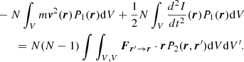
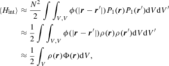
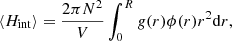
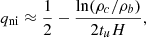
Similarly, the interaction energy of the ensemble of particles ⟨H_int⟩ can be defined by summing all the interaction energies between distinct pairs of particles in the N-body description or by integrating over P₂(r, r′) for the fluid volume,

$$\begin{array}{cc}\hfill ⟨H_{\mathrm{int}}⟩& ={\displaystyle \sum _{i<j}}\varphi (|{\mathit{r}}_i-{\mathit{r}}_j|)\hfill \\ \hfill & =\frac{N(N-1)}{2}{\displaystyle \int {\int }_{V,V}}\varphi (|\mathit{r}-{\mathit{r}}^{\prime }|)P_2(\mathit{r},{\mathit{r}}^{\mathbf{\prime }})\mathrm{d}V\mathrm{d}{V}^{\prime },\hfill \end{array}$$(3)

where N(N − 1)/2 is the number of independent pairs in the fluid. In the homogeneous and isotropic case, P₂(r, r′) only depends on the distance modulus ||r − r′||. It is then convenient to define the radial distribution function

$$\begin{array}{c}\hfill g(||\mathit{r}-{\mathit{r}}^{\mathbf{\prime }}||)=V^2{P}_2(\mathit{r},{\mathit{r}}^{\mathbf{\prime }}),\end{array}$$(4)

or equivalently, the correlation function, ξ(||r − r′||), for a homogeneous isotropic fluid,

$$\begin{array}{cc}\hfill \xi (||\mathit{r}-{\mathit{r}}^{\mathbf{\prime }}||)& =V^2(P_2(\mathit{r},{\mathit{r}}^{\mathbf{\prime }})-P_1(\mathit{r})P_1({\mathit{r}}^{\mathbf{\prime }}))\hfill \\ \hfill & =V^2{P}_2(\mathit{r},{\mathit{r}}^{\mathbf{\prime }})-1\hfill \\ \hfill & =g(||\mathit{r}-{\mathit{r}}^{\mathbf{\prime }}||)-1.\hfill \end{array}$$(5)

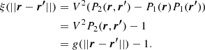
For an isotropic fluid, the correlation function ξ(r) is the angle-averaged value of ξ(r)=⟨δ(r′)δ(r + r′)⟩, with δ(r) the density perturbation defined as δ(r)=(ρ(r)−⟨ρ⟩)/⟨ρ⟩) (see Springel et al. 2017). Here, ⟨ ⋅ ⟩ denotes a volume average. The power spectrum can then be defined as the Fourier transform of ξ(r),

$$\begin{array}{c}\hfill \xi (\mathit{r})=\frac{V}{{(2\pi )}^3}{\displaystyle \int {|{\delta }_{\mathit{k}}|}^2}{e}^{-i\mathit{k}·\mathit{r}}{d}^{3}k,\end{array}$$(6)

which is commonly used in cosmological studies to characterize the large-scale structures of the Universe (Peebles 1980; Peacock 1999). We show here that the correlation function is not a simple diagnostic of structures, but plays an active role in determining the dynamics of the fluid. For the sake of similarity with the tools that are commonly used in statistical physics, we use the radial distribution function rather than the correlation function in our calculations.

It is easy to see that in the absence of correlation in the fluid, P₂(r, r′)=P₁(r)P₁(r′), that is, ξ(||r − r′||)=0 and g(||r − r′||)=1 for all r and r′ in the case of a homogeneous fluid. This situation is the limit case of an ideal fluid, often referred to as “perfect molecular chaos”, for which the radial distribution function is equal to 1 everywhere. A schematic representation of such an ideal and homogeneous fluid is given in the left panel of Fig. 1, where the blue dots represent point-like interactionless particles. In this example, the fluid is homogeneous at all scales: the density inside a small (V₁) or large (V₂) control volume is independent of the location of the control volume.

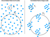Fig. 1. Schematic illustration of situations in which the ideal hypothesis is valid and in which it breaks down. Left: fluid is uncorrelated at all scales. Right: on the scale of control volume V1, the fluid can be considered locally as inhomogeneous and uncorrelated, while on the scale of control volume V2, the fluid can be considered as globally homogeneous and correlated.

In the presence of interactions, the density distribution may no longer be homogeneous at all scales, for instance, in the presence of clustering in the particle distribution. This situation is shown in the right panel of Fig. 1. For a small control volume V₁, the distribution of particles within the volume is ideal and there is no correlation: P₂(r, r′)=P₁(r)P₁(r′). However, the density depends on the location of the control volume, for example, whether it lies within a cluster or outside. This means that inhomogeneities are resolved and the fluid is ideal (i.e., uncorrelated), but inhomogeneous. For a large control volume V₂, the distribution of particles within the volume is not ideal and correlations are induced by the clustering inside the volume: P₂(r, r′)≠P₁(r)P₁(r′). However, the density does not depend on the location of the control volume provided that the control volume is sufficiently large. In that case, the inhomogeneities are not resolved and the fluid is nonideal (correlated) and homogeneous.

This distinction is very important for the correct treatment of inhomogeneities (correlations) in a fluid. Because it depends on the scale, this is of prime importance for astrophysical flows, which can only be observed or simulated at large scales. The main consequence is that we cannot simply average over large volumes as this masks the complexity of the density inhomogeneities: these inhomogeneities then result in correlations in the fluid, which requires a change in dynamical equations. This can be seen with the computation of the interaction energy, which intrinsically depends on the distance between particles (see Eq. (3)). Within a statistical (fluid) description, the interaction energy fundamentally involves the pair correlation function, P₂(r, r′)≠P₁(r)P₁(r′). In a simulation assuming an ideal fluid, the correlations will be missed, that is, the fluid at small scales may erroneously be considered as ideal if correlations are present. This yields an erroneous estimate of the interaction energy. The proper calculation of the interaction energy must thus be done accurately and ensure that the small-scale interaction energy is properly accounted for. This may be done through Eq. (3) and the use of a nonideal framework.

2.2. Virial theorem for correlated fluids

For a system of interacting particles of mass m, the N-body form of the virial theorem can be stated as

$$\begin{array}{c}\hfill -{\displaystyle \sum _i}m{\mathit{v}}_i^2+\frac{1}{2}{\displaystyle \sum _i}\frac{d^2{I}_i}{d{t}^2}={\displaystyle \sum _{i,j,i\ne j}}{\mathit{F}}_{j\to i}·{\mathit{r}}_i,\end{array}$$(7)

where $I_i=m{r}_i^2$ is the moment of inertia of the particle i. In a fluid (statistical) approach, the equivalent form reads

$$\begin{array}{cc}& -N{\displaystyle {\int }_V}m{\mathit{v}}^2(\mathit{r})P_1(\mathit{r})\mathrm{d}V+\frac{1}{2}N{\displaystyle {\int }_V}\frac{d^{2}I}{d{t}^2}(\mathit{r})P_1(\mathit{r})\mathrm{d}V\hfill \\ \hfill & =N(N-1){\displaystyle \int {\int }_{V,V}}{\mathit{F}}_{{\mathit{r}}^{\prime }\to \mathit{r}}·\mathit{r}{P}_2(\mathit{r},{\mathit{r}}^{\prime })\mathrm{d}V\mathrm{d}{V}^{\prime }.\hfill \end{array}$$(8)

Assuming a force deriving from a potential ϕ ∝ |r − r′|^α, the last integral can be symmetrized by using P₂(r, r′) = P₂(r′,r) to obtain

$$\begin{array}{cc}\hfill N(N-1)& {\displaystyle \int {\int }_{V,V}}{\mathit{F}}_{{\mathit{r}}^{\prime }\to \mathit{r}}·\mathit{r}{P}_2(\mathit{r},{\mathit{r}}^{\prime })\mathrm{d}V\mathrm{d}{V}^{\prime }\hfill \\ \hfill & =\frac{N(N-1)}{2}{\displaystyle \int {\int }_{V,V}}{\mathit{F}}_{{\mathit{r}}^{\prime }\to \mathit{r}}·(\mathit{r}-{\mathit{r}}^{\prime })P_2(\mathit{r},{\mathit{r}}^{\prime })\mathrm{d}V\mathrm{d}{V}^{\prime }\hfill \\ \hfill & =-\alpha \frac{N(N-1)}{2}{\displaystyle \int {\int }_{V,V}}\varphi (|\mathit{r}-{\mathit{r}}^{\prime }|)P_2(\mathit{r},{\mathit{r}}^{\prime })\mathrm{d}V\mathrm{d}{V}^{\prime },\hfill \end{array}$$(9)

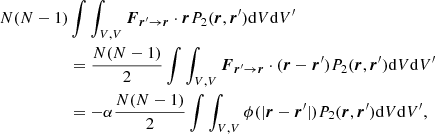
in which we recognize the interaction energy defined in Eq. (3). The virial theorem now takes the classic form

$$\begin{array}{c}\hfill ⟨m{v}^2⟩-\alpha ⟨H_{\mathrm{int}}⟩=\frac{⟨d^{2}I/d{t}^2⟩}{2},\end{array}$$(10)

in which we note the presence of the pair correlation function in the interaction energy.

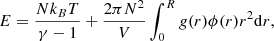
Similarly, we can define the total mechanical energy E_m of the N-body ensemble of particles,

$$\begin{array}{cc}\hfill E_m& =⟨m{\mathit{v}}^2/2⟩+⟨H_{\mathrm{int}}⟩\hfill \\ \hfill & =\frac{1}{2}{\displaystyle \sum _i}m{\mathit{v}}_i^2+{\displaystyle \sum _{i<j}}\varphi (|{\mathit{r}}_i-{\mathit{r}}_j|),\hfill \end{array}$$(11)

whose fluid counterpart is given by

$$\begin{array}{c}\hfill E_m=\frac{N}{2}{\displaystyle {\int }_V}m{\mathit{v}}^2(\mathit{r})P_1(\mathit{r})\mathrm{d}V+\frac{N(N-1)}{2}{\displaystyle \int {\int }_{V,V}}\varphi (|\mathit{r}-{\mathit{r}}^{\prime }|)P_2(\mathit{r},{\mathit{r}}^{\prime })\mathrm{d}V\mathrm{d}{V}^{\prime }.\end{array}$$(12)

If we neglect correlations in the interaction energy, then P₂(r, r′)=P₁(r)P₁(r′), which in the limit N ≫ 1 yields

$$\begin{array}{cc}\hfill ⟨H_{\mathrm{int}}⟩& \approx \frac{N^2}{2}{\displaystyle \int {\int }_{V,V}}\varphi (|\mathit{r}-{\mathit{r}}^{\prime }|)P_1(\mathit{r})P_1({\mathit{r}}^{\prime })\mathrm{d}V\mathrm{d}{V}^{\prime }\hfill \\ \hfill & \approx \frac{1}{2}{\displaystyle \int {\int }_{V,V}}\varphi (|\mathit{r}-{\mathit{r}}^{\prime }|)\rho (\mathit{r})\rho ({\mathit{r}}^{\prime })\mathrm{d}V\mathrm{d}{V}^{\prime }\hfill \\ \hfill & \approx \frac{1}{2}{\displaystyle {\int }_V}\rho (\mathit{r})\mathrm{\Phi }(\mathit{r})\mathrm{d}V,\hfill \end{array}$$(13)

where we have defined the mean-field potential Φ(r)=∫_Vϕ(|r − r′|)ρ(r′)dV′, which can be computed with the Poisson equation for the gravitational or the electrostatic force, ∇²Φ(r)∝ρ(r). However, we stress that the possibility of defining this mean-field potential is only possible in the absence of correlations: as soon as P₂(r, r′)≠P₁(r)P₁(r′), the use of a mean-field and the Poisson equation is not correct as it will ignore the correlations present in the system.

2.3. Newton’s laws of motion for pressureless correlated fluids

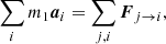
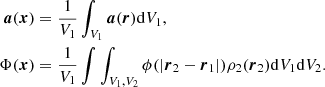
At a more fundamental level, we can also show that correlations should be taken into account in Newton’s laws for a (pressureless) correlated fluid. We consider now an ensemble of N₁ particles of mass m₁ in a volume V₁ interacting with N₂ particles of mass m₂ in a volume V₂ (see Fig. 2). In an N-body approach, the second law can be written

$$\begin{array}{c}\hfill {\displaystyle \sum _i}{m}_1{\mathit{a}}_i={\displaystyle \sum _{j,i}}{\mathit{F}}_{j\to i},\end{array}$$(14)

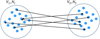Fig. 2. Schematic illustrating the interactions between two fluid volumes used to derive Newton’s laws for pressureless correlated fluids.

with i in [0, N₁] and j in [0, N₂]. Newton’s second law for a pressureless correlated fluid is then given by

$$\begin{array}{c}\hfill N_1{\displaystyle {\int }_{V_1}}{m}_1\mathit{a}(\mathit{r})P_1(\mathit{r})\mathrm{d}{V}_1=N_1{N}_2{\displaystyle \int {\int }_{V_1,V_2}}{\mathit{F}}_{{\mathit{r}}_2\to {\mathit{r}}_1}{P}_2({\mathit{r}}_1,{\mathit{r}}_2)\mathrm{d}{V}_1\mathrm{d}{V}_2,\end{array}$$(15)

which we write in a more compact way as ⟨m₁a⟩₁ = ⟨F⟩_2 → 1. We have generalized the two-point probability density function to different volumes V₁ and V₂ , and it is normalized by N₁N₂.

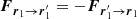The first law for an isolated fluid of volume V₁ is then ⟨m₁a⟩₁ = ⟨F⟩_1 → 1 = 0 and can be deduced from the second law by taking V₂ = V₁ and using $P_2({\mathit{r}}_1,{\mathit{r}}_1^{\mathrm{\prime }})=P_2({\mathit{r}}_1^{\mathrm{\prime }},{\mathit{r}}_1)$ and ${\mathit{F}}_{{\mathit{r}}_1\to {\mathit{r}}_1^{\mathrm{\prime }}}=-{\mathit{F}}_{{\mathit{r}}_1^{\mathrm{\prime }}\to {\mathit{r}}_1}$. Similarly, the third law ⟨F⟩_2 → 1 = −⟨F⟩_1 → 2 can be obtained using the same arguments.

We now assume that there is no correlation, that is, P₂(r₁, r₂)=P₁(r₁)P₁(r₂), and that the fluid is isotropic and homogeneous: P₁(r₁)=1/V₁. Choosing the origin of positions, x, at the center of V₁, we have N₁/V₁ = ρ₁(x) (see Sect. 2.1), and we define

$$\begin{array}{cc}\hfill \mathit{a}(\mathit{x})& =\frac{1}{V_1}{\displaystyle {\int }_{V_1}}\mathit{a}(\mathit{r})\mathrm{d}{V}_1,\hfill \\ \hfill \mathrm{\Phi }(\mathit{x})& =\frac{1}{V_1}{\displaystyle \int {\int }_{V_1,V_2}}\varphi (|{\mathit{r}}_2-{\mathit{r}}_1|){\rho }_2({\mathit{r}}_2)\mathrm{d}{V}_1\mathrm{d}{V}_2.\hfill \end{array}$$(16)

The second law then becomes

$$\begin{array}{cc}\hfill \frac{{\rho }_1(\mathit{x})m_1}{V_1}{\displaystyle {\int }_{V_1}}\mathit{a}(\mathit{r})\mathrm{d}{V}_1& =\frac{{\rho }_1(\mathit{x})m_1}{V_1}{\displaystyle \int {\int }_{V_1,V_2}}\frac{{\mathit{F}}_{{\mathit{r}}_2\to {\mathit{r}}_1}}{m}{\rho }_2({\mathit{r}}_2)\mathrm{d}{V}_1\mathrm{d}{V}_2\hfill \\ \hfill {\rho }_1(\mathit{x})m_1\mathit{a}(\mathit{x})& \approx {\rho }_1(\mathit{x})m_1\frac{-{\mathbf{\nabla }}_{\mathit{x}}\mathrm{\Phi }(\mathit{x})}{m_1},\hfill \end{array}$$(17)

where we recognize the usual form of an external mean force deriving from the mean -field potential Φ(x). In the case of the gravitational force, Φ(x)/m₁ is independent of m₁, and the equivalence principle for a pressureless ideal fluid simply consists of simplifying Eq. (17) by ρ₁(x)m₁ on each side,

$$\begin{array}{c}\hfill \mathit{a}(\mathit{x})\approx \frac{-{\mathbf{\nabla }}_{\mathit{x}}\mathrm{\Phi }(\mathit{x})}{m_1}.\end{array}$$(18)

However, this simplification is only possible in the absence of correlations. That is, as soon as P₂(r, r′)≠P₁(r)P₁(r′), the use of the equivalence principle is not correct as it will ignore the correlations present in the system.

2.4. Nonideal equation of state

We recall that for a homogeneous and isotropic fluid, P₂(r, r′) = g(|r − r′|)/V². In this case (for N ≫ 1), the interaction energy becomes

$$\begin{array}{c}\hfill ⟨H_{\mathrm{int}}⟩=\frac{2\pi N^2}{V}{\displaystyle {\int }_0^R}g(r)\varphi (r)r^2\mathrm{d}r,\end{array}$$(19)

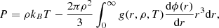
with r = |r − r′| and V = 4πR³/3. Statistical mechanics in the canonical ensemble in thermal equilibrium with a heat bath at a fixed temperature T can be used to define the EOS. We refer to classical textbooks such as Hansen et al. (2006) for details. The energy of the system in the absence of external forces is then given by

$$\begin{array}{c}\hfill E=\frac{N{k}_{B}T}{\gamma -1}+\frac{2\pi N^2}{V}{\displaystyle {\int }_0^R}g(r)\varphi (r)r^2\mathrm{d}r,\end{array}$$(20)

with γ = C_P/C_V the adiabatic index of the fluid, defined as the ratio of the specific heats at constant pressure and volume, respectively (γ = 5/3 for mono-atomic particles in their ground state). The first term in Eq. (20) is the perfect gas contribution, and the second term stems from the interactions between particles. The nonideal pressure is given by

$$\begin{array}{c}\hfill PV=N{k}_{B}T-\frac{2\pi N^2}{3V}{\displaystyle {\int }_0^R}g(r)\frac{d\varphi (r)}{\mathrm{d}}r{r}^3\mathrm{d}r.\end{array}$$(21)

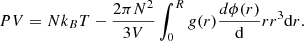
When the temperature is identified with the velocity dispersion of particles within the fluid (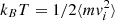$k_{B}T=1/2⟨m{v}_i^2⟩$), Eq. (21) can be interpreted as the isotropic form of the virial theorem. P = 0 corresponds to virial equilibrium, for which the ideal pressure is balanced by the interaction contribution. P >  0 corresponds to a fluid that expands because either the ideal (kinetic) pressure dominates the interaction term or the interactions are repulsive, dϕ(r)/dr <  0. In contrast, P <  0 corresponds to a fluid that collapses because the contribution due to attractive interactions dϕ(r)/dr >  0 dominates the ideal pressure. This case corresponds to a phase transition from gas to liquid, for instance, with the attractive interactions being the intermolecular dipole forces, or to gravitational collapse in the case of the gravitational force (see, e.g., de Vega & Sánchez 2002).

Strictly speaking, a self-interacting fluid should always be described with a nonideal EOS. Nevertheless, an ideal approximation is possible if the interaction term is negligible in Eq. (21). In this case, g(r)≈1, so that with ρ = N/V, the condition becomes

$$\begin{array}{c}\hfill \rho k_{B}T\gg \frac{2\pi {\rho }^2}{3}{\displaystyle {\int }_0^R}\frac{d\varphi (r)}{\mathrm{d}}r{r}^3\mathrm{d}r.\end{array}$$(22)

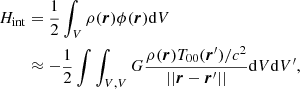
For a potential of the form ϕ = −k/r (with k >  0 for the gravitational force or attractive Coulomb interactions),

$$\begin{array}{c}\hfill \rho k_{B}T\gg \pi {\rho }^{2}k{R}^2/3\Rightarrow R\ll \sqrt{\frac{k_{B}T}{k\rho }}.\end{array}$$(23)

In this case, we recognize the characteristic Debye screening length in the case of Coulomb interactions or the Jeans length in the case of the gravitational force. The condition in Eq. (23) states that an ideal approximation in the treatment of the fluid under consideration is acceptable if (and only if) the volumes considered are sufficiently small so that the Debye length or the Jeans length is well resolved. Whereas such a condition is usually fulfilled in numerical simulations of star formation and is known as the Truelove condition (see Truelove et al. 1997), it is not easily done for large-scale numerical simulations of galaxies or larger structures. In these cases, it is mandatory to use a nonideal EOS and to include the terms involving the pair-correlation function in the calculations in this way.

2.5. Nonideal stress tensor

More generally, we express the above theory in the form of a stress tensor, following the pioneering work of Kirkwood et al. (1949). The Newtonian expression for the stress tensor of a system of N particles of mass m is given by

$$\begin{array}{c}\hfill {\sigma }_{\mathit{ij}}=-(P+(\frac{2}{3}\eta -\chi ){\displaystyle \sum _k}{\partial }_k{u}_k){\delta }_{\mathit{ij}}+\eta ({\partial }_i{u}_j+{\partial }_j{u}_i),\end{array}$$(24)

with P the nonideal pressure given in Sect. 2.4, and η and χ the coefficients of shear and bulk viscosity, which can be computed as

$$\begin{array}{cc}\hfill \eta & =\frac{1}{2}\frac{N}{V}mD+\frac{\pi }{15D}\frac{N^2}{V^2}{\displaystyle {\int }_0^R}{\psi }_2(r)g(r)\frac{d\varphi (r)}{\mathrm{d}}r{r}^3\mathrm{d}r,\hfill \\ \hfill \chi & =\frac{1}{3}\frac{N}{V}mD+\frac{\pi }{9D}\frac{N^2}{V^2}{\displaystyle {\int }_0^R}{\psi }_0(r)g(r)\frac{d\varphi (r)}{\mathrm{d}}r{r}^3\mathrm{d}r,\hfill \end{array}$$(25)

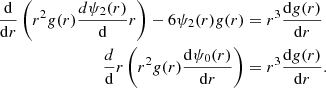
with D the self-diffusion coefficient in the fluid (from Fick’s law). As defined in Kirkwood et al. (1949), ψ₀(r) is the surface harmonic of zeroth order arising from the dilatation component of the rate of strain, and ψ₂(r) is the surface harmonic of order 2 arising from the shear component. They obey the following differential equations:

$$\begin{array}{cc}\hfill \frac{\mathrm{d}}{\mathrm{d}r}\left(r^{2}g(r)\frac{d{\psi }_2(r)}{\mathrm{d}}r\right)-6{\psi }_2(r)g(r)& =r^3\frac{\mathrm{d}g(r)}{\mathrm{d}r}\hfill \\ \hfill \frac{d}{\mathrm{d}}r\left(r^{2}g(r)\frac{\mathrm{d}{\psi }_0(r)}{\mathrm{d}r}\right)& =r^3\frac{\mathrm{d}g(r)}{\mathrm{d}r}.\hfill \end{array}$$(26)

As for the nonideal pressure, the nonideal coefficients of shear and bulk viscosity contain two contributions: an ideal (Brownian) contribution arising from the momentum transfer between colliding particles, and a nonideal part arising from the direct transfer by interaction forces. The second part strongly dominates when interactions are present in the fluid. As for the nonideal pressure, it is also crucial to take interactions in the stress tensor into account when the Jeans length is not resolved.

2.6. Thermodynamic limit

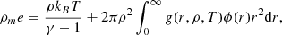
We can take the thermodynamic limit by imposing (N, V)→∞ while keeping N/V = ρ constant. Defining ρ_me the internal energy per unit volume (with ρ_m = ρm),

$$\begin{array}{c}\hfill P=\rho k_{B}T-\frac{2\pi {\rho }^2}{3}{\displaystyle {\int }_0^{\infty }}g(r,\rho ,T)\frac{\mathrm{d}\varphi (r)}{\mathrm{d}r}{r}^3\mathrm{d}r,\end{array}$$(27)

$$\begin{array}{c}\hfill {\rho }_{m}e=\frac{\rho k_{B}T}{\gamma -1}+2\pi {\rho }^2{\displaystyle {\int }_0^{\infty }}g(r,\rho ,T)\varphi (r)r^2\mathrm{d}r,\end{array}$$(28)

where we have made the dependence of the radial distribution function on the external variables ρ and T explicit. Determining the EOS now reduces to the determination of g(r, ρ, T), which can be done by three different technics in the case of liquids: calculation of the Ornstein-Zernike equation, N-body Monte Carlo or molecular dynamic simulations, or experiments by X-ray or neutron diffraction (see Aslangul 2006). We emphasize that we implicitly assume here that an equilibrium can be reached. This allows us to define a radial distribution function that does not depend on time and can be determined from external variables (ρ and T). Strictly speaking, this might not be the case for self-gravitating systems that are collapsing, hence are not in equilibrium. This assumption then assumes that some sort of feedback stabilizes small scales, allowing for the definition of an EOS for the scales that are not resolved and described by statistical mechanics. This assumption can be relaxed when the dynamical equations in the BBGKY hierarchy are used that describe the evolution of the correlations. However, as discussed in Davis & Peebles (1977), we need to find a closure relation for the hierarchy by expressing the last N-point correlation functions as a function of the others. This closure is likely possible only at very high N in order to accurately describe the structures that are observed in the Universe (see Balian & Schaeffer 1989a,b), which would result in a complex system of dynamical equations describing the evolution of correlations. We therefore use here a pragmatic approach (similarly to the approach used for liquids in physical chemistry) and assume that an equilibrium, or more exactly, a stationary state, exists at small scales. We also assume that we can determine the two-point correlation function either by explicitly resolving inhomogeneities in small-scale numerical simulations (e.g., with molecular dynamics for liquids or N-body simulations for self-gravitating systems) or by using astrophysical observations.

An important point is that the thermodynamic limit in Eq. (28) is well defined only if we obtain an extensive definition of the total internal energy E (or intensive for the internal energy density per unit volume ρ_me), that is, the integral in the expression must converge when N, V → ∞. Because lim_{r → ∞}g(r)=1, this means that the potential from which the force derives must decrease faster than r⁻⁴ at infinity. This is the case for the Lennard-Jones potential, which is classically used to model intermolecular forces in liquid water or molecular liquids. An interpretation of this requirement is that the interaction energy in Eq. (20) is not proportional to N² but to N × N_neighbors, with N_neighbors the number of particles involved in the short-range interactions. Therefore, the interaction energy is proportional to N and the definition of E is extensive in the thermodynamic limit. If the interactions are long range, however, the interaction energy is really proportional to N². In this case, the total energy E is not extensive, and we cannot use the thermodynamic limit. This problem is usually thought to prevent the use of statistical mechanics to describe systems characterized by a long-range force, such as gravity. We show in Sect. 3 a correct treatment in the case of the gravitational force.

3. Nonideal self-gravity

3.1. Hierarchical virial theorem

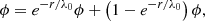
As we showed in Sect. 2.4, characteristic length scales such as the Debye length λ_D or Jeans length λ_J can be defined to determine whether nonideal (interaction) contributions should be taken into account. In the case of the electrostatic force, the Coulomb potential is split into a short-range and a long-range component, ϕ = exp(−r/λ_D)ϕ + (1 − exp(−r/λ_D))ϕ. The first part corresponds to the screened Coulomb potential, due to the polarizable electron background, and the residual corresponds to the departure between the Coulomb and the screened potential (e.g., Chabrier 1990). We propose to decompose the gravitational force in a similar manner.

Hydrogen atoms become gravitationally bounded in the interior of a star, for example. Using a classical polytropic stellar model, we can define a virial theorem that balances the internal energy in the star and the gravitational interaction energy (see, e.g., Sect. 4.1). If now we consider a cluster of interacting polytropic stars, we can consider each star as isolated in a first approximation and use the previous virial theorem to obtain their internal structure and then describe their collective dynamics assuming they are point masses (i.e., we neglect tidal interactions). However, we can easily see that we should not integrate the gravitational force at infinity when using the virial theorem in a single star, otherwise we would include some gravitational interactions in the internal stellar structures that contribute to the cluster dynamics. A solution for this issue is to decompose the gravitational potential into a near-field and far-field component using a length scale λ₀ larger than the size of a star,

$$\begin{array}{c}\hfill \varphi =e^{-r/{\lambda }_0}\varphi +(1-e^{-r/{\lambda }_0})\varphi ,\end{array}$$(29)

and we apply the virial theorem inside a star using the near-field ϕ₀ = exp(−r/λ₀)ϕ. We emphasize that the use of exponential damping is arbitrary. Another possibility is to use an erf function, as is often done with the Coulomb interaction in physical chemistry. We can then proceed recursively in the residual part. We now use a second length scale λ₁ in order to define a near field ϕ₁ for the virial theorem describing the dynamics inside the stellar cluster and a far field for the dynamics of a collection of stellar clusters inside a galaxy, for example. ϕ₁ is then given by exp(−r/λ₁)(1 − exp(−r/λ₀))ϕ. We can continue to define the gravitational energy contributing to the dynamics of the stellar clusters inside the galaxy and then the dynamics of the galaxies inside a galaxy cluster, and so on. The hierarchical decomposition of the gravitational potential with a collection of length scales λ₀,... λ_i... is then given by

$$\begin{array}{cc}\hfill \varphi & ={\displaystyle \sum _{i=0}^{\infty }}{\varphi }_i\hfill \\ \hfill {\varphi }_i& =e^{-r/{\lambda }_i}{\displaystyle \prod _{j=0}^{i-1}}(1-e^{-r/{\lambda }_j})\varphi .\hfill \end{array}$$(30)

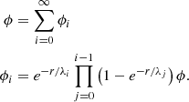
This expansion is similar to the BBGKY hierarchy for the N-body problem in statistical physics, where the potential is split into a (short-range) interparticle pair potential and a (long-range) external-field potential (see, e.g., Chavanis 2013). The series of length scales is a-priori arbitrary, and for a purely self-gravitating collapsing fluid, there is no particular length scale that would physically make sense. The characteristic length scales that should be used are likely linked to feedback and support processes that define the possible virial equilibria at different scales: active galactic nucleus feedback for galaxy clusters, rotational support for galaxies, stellar feedback for molecular clouds and star clusters, and pressure support for stars. When this stationary state is reached, for instance, inside a star, we can account for the velocity dispersion and gravitational energy at this scale as internal degrees of freedom (similarly to an EOS) when going to a larger scale. When tidal effects are neglected, this allows decoupling the different scales based on feedback processes.

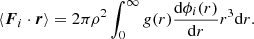
We can now use the virial theorem defined in Sect. 2.2 to link the dynamic properties v_i, I_i of objects of mass m_i at each scale λ_i of the hierarchy to the corresponding gravitational interaction potential ϕ_i,

$$\begin{array}{c}\hfill -⟨m_i{v}_i^2⟩+⟨d^2{I}_i/d{t}^2⟩/2=⟨{\mathit{F}}_i·\mathit{r}⟩,\end{array}$$(31)

in which we can replace kinetic energy by thermal energy for i = 0. As mentioned above, we emphasize that this hierarchy neglects tidal interactions. A possible extension would be to also decompose the energy going into tides, if they are not negligible at a given scale. This is likely to be the case at the scale of galaxies (see, e.g., Barnes & Hernquist 1992). For the time being, however, we assume that these contributions represent a small correction to the total gravitational energy.

Because each term ⟨F_i ⋅ r⟩ is computed with the short-range potential ϕ_i, damped by a factor e^−r/λ_i, we can now safely take the thermodynamic limit in Eq. (31), that is, N, V → ∞, because the integral converges. For a homogeneous and isotropic correlated fluid, this term is given by

$$\begin{array}{c}\hfill ⟨{\mathit{F}}_i·\mathit{r}⟩=2\pi {\rho }^2{\displaystyle {\int }_0^{\infty }}g(r)\frac{\mathrm{d}{\varphi }_i(r)}{\mathrm{d}r}{r}^3\mathrm{d}r.\end{array}$$(32)

Similarly, the total mechanical energy of the system at a scale λ_i is given by

$$\begin{array}{c}\hfill E_{m,i}=⟨m_i{v}_i^2/2⟩+⟨H_{\mathrm{int},i}⟩,\end{array}$$(33)

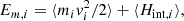
where we can take the thermodynamic limit for the interaction energy,

$$\begin{array}{c}\hfill ⟨H_{\mathrm{int},i}⟩=2\pi {\rho }^2{\displaystyle {\int }_0^{\infty }}g(r){\varphi }_i(r)r^2\mathrm{d}r.\end{array}$$(34)

We show in the next section that a similar decomposition can be used to define nonideal self-gravitating hydrodynamics in numerical simulations.

3.2. Nonideal self-gravitating hydrodynamics

A standard strategy to obtain a large-scale hydrodynamic model of complex multiphasic systems relies on the homogenization procedure by averaging volumes of characteristic size λ (Whitaker 1998). We can then decompose the interaction potential into a near-field and a far-field contribution using this characteristic scale. However, in numerical simulations, as soon as the grid size (or the kernel extension in SPH methods) is such that Δx <  λ, inhomogeneities at scales smaller than λ have no physical meaning in such a homogenized model, which is only valid at scales larger than λ.

In numerical simulations, it is then natural to use the grid resolution Δx as the characteristic length to split the gravitational interaction

$$\begin{array}{c}\hfill \varphi (r)=e^{-r/\mathrm{\Delta }x}\varphi (r)+(1-e^{-r/\mathrm{\Delta }x})\varphi (r).\end{array}$$(35)

We can then define a near field ϕ_int(r)=exp(−r/Δx)ϕ(r) to handle the nonideal effects in the EOS inside the simulation control volumes, and a far field ϕ_ext(r)=(1 − exp(−r/Δx))ϕ(r) to define the external force between the simulation control volumes. Following Irving & Kirkwood (1950), the Navier-Stokes equations for a nonideal fluid can be derived from the Liouville equation in the BBGKY hierarchy, and in the case of a self-gravitating fluid, they are given by

$$\begin{array}{cc}\hfill \frac{\partial {\rho }_m}{\partial t}+\mathbf{\nabla }\left({\rho }_m\mathit{u}\right)& =0,\hfill \\ \hfill \frac{\partial {\rho }_m\mathit{u}}{\partial t}+\mathbf{\nabla }({\rho }_m\mathit{u}\otimes \mathit{u}+\sigma )& ={\mathit{F}}_{\mathrm{ext}},\hfill \\ \hfill \frac{\partial {\rho }_{m}E}{\partial t}+\mathbf{\nabla }({\rho }_m\mathit{u}E+\sigma ·\mathit{u})& ={\mathit{F}}_{\mathrm{ext}}·\mathit{u},\hfill \end{array}$$(36)

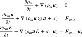
using the following relations for E and σ

$$\begin{array}{cc}\hfill E& =e+\frac{1}{2}{\mathit{u}}^2,\hfill \\ \hfill {\sigma }_{\mathit{ij}}& =-(P+(\frac{2}{3}\eta -\chi ){\displaystyle \sum _k}{\partial }_k{u}_k){\delta }_{\mathit{ij}}+\eta ({\partial }_i{u}_j+{\partial }_j{u}_i),\hfill \end{array}$$(37)

in which the nonideal (internal) quantities are given by

$$\begin{array}{cc}\hfill P& =\rho k_{B}T-\frac{2\pi {\rho }^2}{3}{\displaystyle {\int }_0^{\infty }}g(r)\frac{d{\varphi }_{\mathrm{int}}(r)}{\mathrm{d}r}{r}^3\mathrm{d}r\hfill \\ \hfill {\rho }_{m}e& =\frac{\rho k_{B}T}{\gamma -1}+2\pi {\rho }^2{\displaystyle {\int }_0^{\infty }}g(r){\varphi }_{\mathrm{int}}(r)r^2\mathrm{d}r\hfill \\ \hfill \eta & =\frac{1}{2}{\rho }_{m}D+\frac{\pi }{15D}{\rho }^2{\displaystyle {\int }_0^{\infty }}{\psi }_2(r)g(r)\frac{d{\varphi }_{\mathrm{int}}(r)}{\mathrm{d}r}{r}^3\mathrm{d}r\hfill \\ \hfill \chi & =\frac{1}{3}{\rho }_{m}D+\frac{\pi }{9D}{\rho }^2{\displaystyle {\int }_0^{\infty }}{\psi }_0(r)g(r)\frac{d{\varphi }_{\mathrm{int}}(r)}{\mathrm{d}r}{r}^3\mathrm{d}r\hfill \\ \hfill \mathrm{with}{\varphi }_{\mathrm{int}}(r)& =-\frac{G{m}^2}{r}{e}^{-r/\mathrm{\Delta }x},\hfill \end{array}$$(38)

with ψ₂(r) and ψ₀(r) given by Eq. (26). The external force is defined by an integral form in the whole simulation domain V_sim

$$\begin{array}{cc}\hfill {\mathit{F}}_{\mathrm{ext}}(\mathit{x})& =-\rho (\mathit{x}){\mathbf{\nabla }}_{\mathit{x}}({\mathrm{\Phi }}_{\mathrm{ext}}(\mathit{x})),\hfill \\ \hfill {\mathrm{\Phi }}_{\mathrm{ext}}(\mathit{x})& ={\displaystyle {\int }_{V_{\mathrm{sim}}}}{\varphi }_{\mathrm{ext}}(|\mathit{x}-{\mathit{x}}^{\prime }|)\rho ({\mathit{x}}^{\prime })\mathrm{d}{V}_{\mathrm{sim}},\hfill \\ \hfill \mathrm{with}{\varphi }_{\mathrm{ext}}(r)& =-\frac{G{m}^2}{r}(1-e^{-r/\mathrm{\Delta }x}).\hfill \end{array}$$(39)

As for the virial theorem in the previous section, all the integrals in the EOS quantities are defined with the damped potential ϕ_int(r)=e^−r/Δxϕ(r). Hence, all these integrals are well defined and converge in the thermodynamic limit. When Δx ≪ λ_J and notably in the limit Δx → 0, we have ϕ_int(r)→0 and ϕ_ext(r)→ϕ(r), which means that all the gravitational force is entirely resolved externally and the nonideal contributions to the fluid EOS given by Eq. (38) are negligible: We recover then the classical (ideal) form of the Navier-Stokes equations for a self-gravitating fluid. As soon as Δx >  λ_J, however, the nonideal contributions to the EOS due to interactions within the control volumes must be included for a correct calculation of the gravitational energy of the whole system.

4. Applications

4.1. Impact of inhomogeneities on the virial theorem

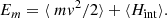
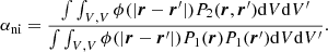
The virial theorem is usually applied in astrophysics in a simplified way. We define the total mass M = Nm, and the average total energy ⟨E/M⟩, kinetic energy ⟨E_kin/M⟩, and potential energy ⟨E_p/M⟩ per unit mass. The virial theorem, assuming that the particles are gravitationally bound in a sphere of radius r_bound, is usually evaluated with these quantities per unit mass

$$\begin{array}{cc}\hfill ⟨E/M⟩& =⟨E_{\mathrm{kin}}/M⟩+⟨E_p/M⟩,\hfill \\ \hfill -2⟨E_{\mathrm{kin}}/M⟩& =⟨E_p/M⟩\approx -\frac{\mathit{GM}}{r_{\mathrm{bound}}}.\hfill \end{array}$$(40)

The use of a radius r_bound is similar to the decomposition into near and far fields that we introduced in Sect. 3.1. It defines a scale up to which the gravitational energy is considered to contribute to the virial balance, while the rest is implicitly assumed to contribute to larger-scale dynamics. However, this form of the virial theorem contains no information about the substructures present within the bound volume: only the total mass and size of the system enters the virial equation. This latter thus ignores nonideal effects due to correlations induced by these substructures.

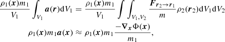
In order to show the importance of inhomogeneities in the virial theorem, we apply it as a simple semianalytical example to the case of a polytropic stellar structure. In this case, we can explicitly compute P₂(r, r′) by semianalytically computing an inhomogeneous density field and compare the result with a homogeneous assumption on the virial theorem. A polytropic stellar structure can be calculated by the Lane-Emden equation,

$$\begin{array}{c}\hfill \frac{1}{z^2}\frac{d}{\mathit{dz}}\left(z^2\frac{\mathit{dw}}{\mathit{dz}}\right)+w^n=0,\end{array}$$(41)

with ρ = ρ_cwⁿ, P = Kρ^γ, n = 1/(γ − 1) the polytropic index, z = Ar, and $A^2=(4\pi G/(n+1)){\rho }_c^{1-1/n}/K$. We choose a dimensionless unit system in which ρ_c = K = G = 1. By solving the Lane-Emden equation for different polytropic indexes n <  5, we can compute inhomogeneous density profiles that have a finite radius R (see the top panel of Fig. 3). For a polytrope, the following virial theorem (per unit mass) reads

$$\begin{array}{cc}\hfill H/M& =2H_{\mathrm{int}}/M,\hfill \\ \hfill H& ={\displaystyle {\int }_V}\frac{\gamma }{\gamma -1}P\mathrm{d}V,\hfill \\ \hfill M& ={\displaystyle {\int }_V}\rho \mathrm{d}V,\hfill \end{array}$$(42)

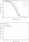Fig. 3. Polytropic solutions. Top: density profiles solutions to the Lane-Emden equation with different polytropic indexes n. Bottom: total enthalpy per unit mass compared to gravitational interaction energy per unit mass assuming either a homogeneous density profile or accounting for inhomogeneities. Blue and green crosses are indistinguishable.

where H is the total enthalpy, M is the total mass, and H_int is given by Eq. (13) with the zero of potential energy defined at the surface of the star. For a homogeneous density profile in Eq. (13), with ρ = M/(4πR³/3), we obtain

$$\begin{array}{c}\hfill \frac{H}{M}=\frac{\mathit{GM}}{5R}.\end{array}$$(43)

For the inhomogeneous case, as illustrated in Fig. 1, there are two possibilities for the description of the inhomogeneities. In the first case (with V₁), they are resolved (e.g., in high – resolution simulations or observations) so that ρ(r) is not constant. In the opposite case (with V₂), ρ(r) is constant and the (unresolved) inhomogeneities are included in the pair correlation function g(r) in our formalism. Determining the impact of ignoring the inhomogeneities thus leads to two different possibilities. For the resolved case, it means comparing the computation with ρ(r) not constant with the computation in which ρ(r) is replaced by its mean value. For the unresolved case, it means comparing the computation with g(r)≠1 with the copmutation assuming an uncorrelated fluid, g(r)=1. The semianalytical polytropic model allows us to easily perform the first (resolved) test. Because we can explicitly compute the inhomogeneous profile ρ(r) and all the necessary integral quantities, we can compare this exact solution with the solution in which ρ(r) is replaced by its mean value.

We now assume that an observer has only access to the total enthalpy, mass, and radius of different objects and does not know whether these objects have substructures. The naive assumption, as explained above, is to ignore the possible inhomogeneities and assume that the density is constant, ρ = M/(4πR³/3), hence using Eq. (43) for the virial equation. This assumption, however, is only correct for a polytropic index n = 0. As shown in the bottom panel of Fig. 3, for profiles n ≠ 0, the error on the total energy is significant and can be up to a factor 25 for n = 4. Therefore, the assumption of a homogeneous profile within the structures will lead to a missing-mass problem. For a polytropic structure, however, we can calculate the inhomogeneous density profile semianalytically and thus calculate exactly the contribution of inhomogeneities to the total energy. We characterize this contribution by an inhomogeneous amplification factor α_ih, which can be calculated exactly,

$$\begin{array}{cc}\hfill {\alpha }_{\mathrm{ih}}& =\frac{N^2{\displaystyle \int {\int }_{V,V}}{P}_2(\mathit{r},{\mathit{r}}^{\prime })\varphi (|\mathit{r}-{\mathit{r}}^{\prime }|)\mathrm{d}V\mathrm{d}{V}^{\prime }}{N^2{\displaystyle \int {\int }_{V,V}}1/{(4\pi R^3/3)}^2\varphi (|\mathit{r}-{\mathit{r}}^{\prime }|)\mathrm{d}V\mathrm{d}{V}^{\prime }}\hfill \\ \hfill & =\frac{{\displaystyle \int {\int }_{V,V}}\rho (r)\rho (r^{\prime })(1/|\mathit{r}-{\mathit{r}}^{\prime }|-1/||\mathit{R}-{\mathit{r}}^{\prime }|)\mathrm{d}V\mathrm{d}{V}^{\prime }}{{\displaystyle \int {\int }_{V,V}}{(M/(4\pi R^3/3))}^2(1/|\mathit{r}-{\mathit{r}}^{\prime }|-1/|\mathit{R}-{\mathit{r}}^{\prime }|)\mathrm{d}V\mathrm{d}{V}^{\prime }},\hfill \end{array}$$(44)

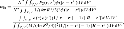
with R a vector on a sphere of radius R (the radius of the polytropic structure), used to define the zero of the gravitational potential at the stellar surface, and V = 4πR³/3. In our calculation, N²P₂(r, r′) = N²P₁(r)P₁(r′) = ρ(r)ρ(r′) for the inhomogeneous structure, while the homogeneous calculation corresponds to N²P₂(r, r′) = N²P₁(r)P₁(r′) = N²/V², with P₁(r)=1/V. We can now correct Eq. (43) to account for inhomogeneities,

$$\begin{array}{c}\hfill \frac{H}{M}=\frac{\mathit{GM}}{5R}{\alpha }_{\mathrm{ih}}.\end{array}$$(45)

As shown in the bottom panel of Fig. 3, when this factor is taken into account, we exactly recover the correct enthalpy and the correct gravitational interaction energy for the different polytropic structures (the green and blue crosses in the figure are indistinguishable). This simple example demonstrates that it is mandatory to account for the contribution of substructures to correctly evaluate interaction energies in astrophysical structures.

4.2. Gravitational viscous regime and the rotation curve of galaxies

Another consequence of substructures and interactions is a possible transition to a viscous regime when interactions dominate at small scales. Heuristically, the rotation curve of a fluid is expected to be strongly impacted by viscous stresses. For high viscosity, the rotation tends to the rotation of a Taylor-Couette flow with u_θ → Ωr in cylindrical coordinates.

We can explore different regimes by performing a Hilbert expansion with a small parameter ϵ that characterizes the regime of the flow, that is, we can take ϵ equal to the inverse of the Reynolds number Re such that ϵ → 0 in the inertial limit. We assume a stationary 2D stellar flow in cylindrical coordinates using either stellar hydrodynamics (see Binney & Tremaine 1987; Burkert & Hensler 1988) or gas hydrodynamics in the HI disk with the nonideal momentum evolution equation presented in Sect. 3.2. In the case of stellar hydrodynamics, we can replace k_BT in Eq. (36) by the velocity dispersion tensor, as is done in the Jeans equation, while the interaction part in the nonideal term remains unchanged. We develop all the variables with respect to ϵ,

$$\begin{array}{cc}\hfill {\rho }_m(r,\theta )& ={\rho }_m^0(r)+ϵ{\rho }_m^1(r,\theta )+...\hfill \\ \hfill u_r(r,\theta )& =ϵu_r^1(r,\theta )+...\hfill \\ \hfill u_{\theta }(r,\theta )& =u_{\theta }^0(r)+ϵu_{\theta }^1(r,\theta )+...\hfill \\ \hfill P(r,\theta )& =P^0(r)+ϵP^1(r,\theta )+...\hfill \\ \hfill {\mathit{F}}_{\mathrm{ext}}(r,\theta )& ={\mathit{F}}_{\mathrm{ext}}^0(r)+ϵ{\mathit{F}}_{\mathrm{ext}}^1(r,\theta )+...\hfill \\ \hfill \eta & ={\eta }^0+ϵ{\eta }^1+...,\hfill \end{array}$$(46)

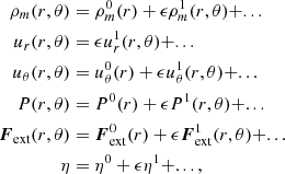
where we have made the hypothesis that the zeroth order is axisymmetric with $u_r^0=0$ and verifies the condition ∇(u⁰)=0.

We can now explore the inertial regime by assuming the following dependence of the shear viscosity and pressure, η⁰ ≈ 0 and P⁰(r)≈0 in the ideal regime, thus with no contribution from interactions. The zeroth order of the nonideal Navier-Stokes equation (Eq. (36)) then gives

$$\begin{array}{cc}\hfill 0^{\mathrm{th}},r-\mathrm{component}:& \frac{-{(u_{\theta }^0)}^2}{r}=\frac{1}{{\rho }_m^0}{F}_{\mathrm{ext},\mathrm{r}}^0\hfill \\ \hfill 0^{\mathrm{th}},\theta -\mathrm{component}:& 0=0,\hfill \end{array}$$(47)

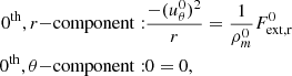
which gives the classical velocity profile $u_{\theta }^0=\sqrt{GM/r}$, decreasing as r^−1/2 at large distance.

In the viscous regime dominated by the nonideal contribution, we now have η⁰ ≠ 0 and P⁰(r)≠0 because of the presence of interactions and bound structures. The zeroth order of the nonideal Navier-Stokes equation then gives

$$\begin{array}{cc}\hfill 0^{\mathrm{th}},r-\mathrm{component}:& \frac{-{(u_{\theta }^0)}^2}{r}=-\frac{1}{{\rho }_m^0}\frac{\partial P^0}{\partial r}+\frac{1}{{\rho }_m^0}{F}_{\mathrm{ext},\mathrm{r}}^0\hfill \\ \hfill 0^{\mathrm{th}},\theta -\mathrm{component}:& 0={\eta }^0(\frac{1}{r}\frac{\partial }{\partial r}\left(r\frac{\partial u_{\theta }^0}{\partial r}\right)-\frac{u_{\theta }^0}{r^2}).\hfill \end{array}$$(48)

We can obtain the velocity profile from the θ component of the Navier-Stokes equation. Under appropriate boundary conditions, the fluid can exhibit a Taylor-Couette flow in the viscous limit: $u_{\theta }^0=\mathrm{\Omega }r$. The associated centrifugal force in the r component is then compensated for by pressure gradients. We recall that the nonideal pressure contains attractive gravitational interactions at small scale here, hence it can compensate for the centrifugal outward acceleration.

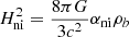
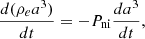
In principle, it should be possible to verify whether this interpretation is correct by exploring such regimes with N-body numerical simulations. The result of this study is presented in Fig. 4 from the N-body simulations of Voglis et al. (2006), who increased the total angular momentum at fixed total mass M and size R, which means that the gravitational energy GM/R is constant for all the simulations. The spiral-arm structures emerge on a scale λ_arm that is smaller than R. When the full N-body dynamics cannot be explored and the simulation is approximated by a fluid, the structure bounded by the spiral arms indicates that the Jeans length is smaller than the size of the system. This implies that a nonideal description is needed when the spiral-arm structures have formed. In this case, the gravitational interactions at small scales inside the spiral arms have to be taken into account in the viscous stress, indicating a transition to the viscous regime. Figure 5 displays the rotation curves associated with the simulations shown in Fig. 4, assuming a half-mass radius of 3 kpc and a total mass of 10¹¹ M_⊙ for the galaxy. A deviation from the inertial regime as soon as spiral-arm structures form is evident. This corroborates the assumption that a transition to a viscous regime occurs.

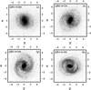Fig. 4. Snapshots of the N-body simulations from Fig. 1 in Voglis et al. (2006). The arm or spiral structures are obtained by increasing the total angular momentum from models QR1 to QR4 for the same mass and size for all the simulations.

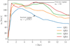Fig. 5. Rotation curves of the different models from QR1 to QR4 from Fig. 2 in Harsoula & Kalapotharakos (2009).

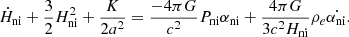
These results also suggest that the change in the rotation curve between spiral and dwarf galaxies and some low surface brightness (LSB) elliptical galaxies exhibiting Keplerian profiles can be interpreted as a phase transition from a nonviscous to a viscous regime that depends on the presence of bound substructures in the galaxy (e.g., local clustering or spiral arms). An example of such a transition is illustrated in Fig. 6 with the observation data of Paolo et al. (2019).

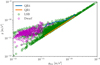Fig. 6. Relation between total acceleration and baryonic component for LSB and dwarf galaxies (Paolo et al. 2019). Acceleration deduced from the rotation curves of models QR1 and QR4 of Voglis et al. (2006) and Harsoula & Kalapotharakos (2009) assuming a half-mass radius of 3 kpc and a total mass of 1011 M⊙ for the galaxy. QR1 is taken as the reference for Keplerian rotation. The bifurcation between Keplerian rotation (QR1) and anomalous rotation (QR4) can be interpreted as a phase transition induced by the presence of substructures, i.e., spiral arms that have developed in model QR4.

4.3. Nonideal cosmology

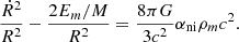
As discussed in Sects. 2.2 and 2.3, the Poisson equation and the equivalence principle can be safely used only for uncorrelated fluids. The Poisson and Einstein equations are not designed to account for (short-scale) correlations that can be present in a fluid. The existence of large-scale structures that have formed during the evolution of the Universe means, however, that we are in the presence of a correlated fluid, even though at very large scales the Universe can be considered as homogeneous and isotropic. It might even be argued that at scales characteristic of these structures, the Universe is the most correlated fluid in nature. Figure 7 shows that the two-point correlation function and radial distribution function can reach values g(r)≈10⁸, to be compared with g(r)=1 for an ideal (uncorrelated) fluid (see Fig. 7). We show below how the effect of these correlations can be incorporated into the Friedmann equations. For simplicity, we restrict ourselves to the Newtonian limit and do not intend to explore an extension of general relativity to the nonideal regime at the moment. It can therefore be considered as a preliminary approach at this stage. As shown in many studies and textbooks (see, e.g., Peacock 1999), however, Newtonian cosmology has proved to be a very useful framework for exploring various physical effects in cosmology while keeping the calculations relatively simple.

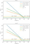Fig. 7. Radial distribution function of stars and gas corresponding to the parameters given in Table 1. Case 1 corresponds to a fit of the correlation functions of the large-scale structures of the Universe at redshift 0 in the IllustrisTNG simulation from Springel et al. (2017). Case 2 uses the same stellar component, but more compact substructures in the gas component.

Assuming a homogeneous and isotropic universe, we can obtain the well-known Friedmann equations from Einstein’s equation,

$$\begin{array}{cc}\hfill H^2+\frac{K}{a^2}& =\frac{8\pi G}{3c^2}{\rho }_e,\hfill \\ \hfill \dot{H}+\frac{3}{2}{H}^2+\frac{K}{2a^2}& =-\frac{4\pi G}{c^2}P,\hfill \end{array}$$(49)

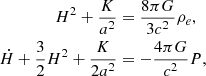
with ρ_e and P the energy density and pressure, H = ȧ(t)/a(t) the Hubble parameter, K the Gaussian curvature, and a(t) the scale factor defining the geometry of the Universe, with ds² = a(t)²dΣ² − c²dt² and dΣ² = dr²/(1 − Kr²)+r²dΩ². We consider flat geometries, with K = 0, and we define the deceleration parameter 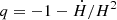$q=-1-\dot{H}/H^2$. The Friedmann equations are then given by

$$\begin{array}{cc}\hfill H^2& =\frac{8\pi G}{3c^2}{\rho }_b,\hfill \\ \hfill q& =-1-\frac{\dot{H}}{H^2}\approx \frac{1}{2},\hfill \end{array}$$(50)

with ρ_b the energy density of baryons. Based on the observed density of baryons, the expansion from the Hubble parameter should be about 15 km⁻¹ s⁻¹ Mpc⁻¹ and the deceleration parameter close to 1/2. As a consequence, this model cannot account for the observed expansion of the Universe close to 67 km/s/Mpc from the latest data of the Planck mission (Planck Collaboration VI 2020), and the acceleration of the expansion measured by type Ia supernovae (Riess et al. 1998), q = −1.0 ± 0.4.

To account for these discrepancies, the standard cosmological model must invoke the presence of cold dark matter (CDM) and dark energy in the form of a cosmological constant Λ, leading to the equations

$$\begin{array}{cc}\hfill H^2& =\frac{8\pi G}{3c^2}({\rho }_b+{\rho }_{\mathrm{CDM}})+\frac{\mathrm{\Lambda }{c}^2}{3},\hfill \\ \hfill q& =-1-\frac{\dot{H}}{H^2}\approx \frac{1}{2}-\frac{\mathrm{\Lambda }{c}^2}{2H}.\hfill \end{array}$$(51)

This adjustment leads to the classical energy budget of the Universe in which baryonic matter accounts for ∼5%, cold dark matter for ∼20%, and dark energy (Λ) for ∼75%.

We now show how correlations can be included in the Friedmann equations. As mentioned above, we present the approach within the Newtonian limit to illustrate our point here. Following Peacock (1999), we assume an ensemble of particles of mass m in a volume V of radius R, whose fluid density is assumed to be homogeneous and isotropic at very large scales, but can be correlated at smaller scales, that is P₁(r)=1/V but P₂(r, r′) ≠ P₁(r)P₁(r′). The total mechanical energy of this system under its N-body or fluid form is given by (see Sect. 2.2)

$$\begin{array}{c}\hfill E_m=⟨m{v}^2/2⟩+⟨H_{\mathrm{int}}⟩.\end{array}$$(52)

Similarly to α_ih in Sect. 4.1, we define α_ni by

$$\begin{array}{c}\hfill {\alpha }_{\mathrm{ni}}=\frac{{\displaystyle \int {\int }_{V,V}}\varphi (|\mathit{r}-{\mathit{r}}^{\prime }|)P_2(\mathit{r},{\mathit{r}}^{\prime })\mathrm{d}V\mathrm{d}{V}^{\prime }}{{\displaystyle \int {\int }_{V,V}}\varphi (|\mathit{r}-{\mathit{r}}^{\prime }|)P_1(\mathit{r})P_1({\mathit{r}}^{\prime })\mathrm{d}V\mathrm{d}{V}^{\prime }}.\end{array}$$(53)

The ideal (uncorrelated) fluid hypothesis corresponds to α_ni = 1. Equation (52) can then be rewritten as

$$\begin{array}{c}\hfill E_m=⟨m{v}^2/2⟩+{\alpha }_{\mathrm{ni}}⟨H_{\mathrm{int},\mathrm{ideal}}⟩.\end{array}$$(54)

Following Peacock (1999), we take 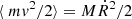$⟨m{v}^2/2⟩=M{\dot{R}}^2/2$ and ⟨H_int, ideal⟩= − GM²/R and rewrite this equation as

$$\begin{array}{c}\hfill E_m/M=\frac{{\dot{R}}^2}{2}-\frac{4\pi }{3}{\alpha }_{\mathrm{ni}}G{\rho }_m{R}^2.\end{array}$$(55)

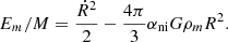
Rearranging the different terms, we obtain

$$\begin{array}{c}\hfill \frac{{\dot{R}}^2}{R^2}-\frac{2E_m/M}{R^2}=\frac{8\pi G}{3c^2}{\alpha }_{\mathrm{ni}}{\rho }_m{c}^2.\end{array}$$(56)

In the uncorrelated case, α_ni = 1, and with the substitutions R → a and −E_m/M → K, we recognize the first Friedmann equation in Eq. (50). Therefore, Eq. (56) indicates that correlations should be accounted for through a multiplicative factor α_ni of the energy density for a proper nonideal generalization of the Friedmann equation (this could also be seen as a multiplicative factor of the gravitational constant). The last step in obtaining a nonideal first Friedmann equation is to take the thermodynamic limit in α_ni, (N, V)→∞ keeping N/V = ρ constant. This can be done by introducing a near-field approximation on a scale λ_H, that is, by replacing ϕ by exp(−r/λ_H)ϕ in Eq. (53), or equivalently, introducing a cutoff of the integrals at a radius r_bound of approximately λ_H. In the latter case, and assuming a large-scale flat, homogeneous, and isotropic Universe, we obtain the following first nonideal Friedmann equation:

$$\begin{array}{c}\hfill H_{\mathrm{ni}}^2=\frac{8\pi G}{3c^2}{\alpha }_{\mathrm{ni}}{\rho }_b\end{array}$$(57)

with

$$\begin{array}{c}\hfill {\alpha }_{\mathrm{ni}}=\frac{{\displaystyle {\int }_0^{r_{\mathrm{bound}}}}g(r)r\mathrm{d}r}{{\displaystyle {\int }_0^{r_{\mathrm{bound}}}}r\mathrm{d}r}.\end{array}$$(58)

We can now study the acceleration of the expansion. Because we can link the value of the Hubble parameter to the nonideal amplification induced by bound substructures, α_ni, it is natural to expect an acceleration of the expansion linked to an increase in the densities of these structures, due to the ongoing gravitational collapse. In order to derive the second nonideal Friedmann equation, we use the first law of thermodynamics in an expanding universe,

$$\begin{array}{c}\hfill \frac{d({\rho }_e{a}^3)}{\mathit{dt}}=-P_{\mathrm{ni}}\frac{d{a}^3}{\mathit{dt}},\end{array}$$(59)

where P is a nonideal pressure. This yields the relation $\dot{{\rho }_e}+3\dot{a}/a{\rho }_e=-3P\dot{a}/a$. Using this relation and the derivation of the first nonideal Friedmann relation, we obtain the nonideal second Friedmann equation,

$$\begin{array}{c}\hfill {\dot{H}}_{\mathrm{ni}}+\frac{3}{2}{H}_{\mathrm{ni}}^2+\frac{K}{2a^2}=\frac{-4\pi G}{c^2}{P}_{\mathrm{ni}}{\alpha }_{\mathrm{ni}}+\frac{4\pi G}{3c^2{H}_{\mathrm{ni}}}{\rho }_e\dot{{\alpha }_{\mathrm{ni}}}.\end{array}$$(60)

Assuming a flat geometry, K = 0, we obtain the deceleration parameter as

$$\begin{array}{c}\hfill q_{\mathrm{ni}}=\frac{1}{2}+\frac{4\pi G}{c^2{H}_{\mathrm{ni}}}{P}_{\mathrm{ni}}{\alpha }_{\mathrm{ni}}-\frac{\dot{{\alpha }_{\mathrm{ni}}}}{2H_{\mathrm{ni}}{\alpha }_{\mathrm{ni}}}.\end{array}$$(61)

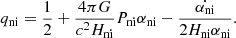
The nonideal pressure term is negligible as in the ideal case. However, we can obtain a negative deceleration parameter with the third term because of $\dot{{\alpha }_{\mathrm{ni}}}$, which is positive because the densities of substructures increase with time due to the ongoing gravitational collapse. This term can then replace the contribution of the cosmological constant that needs to be introduced in the Friedmann equations to explain the acceleration of the expansion in the standard ΛCDM approach.

To summarize, the two nonideal Friedmann equations (for K = 0) in our formalism are given by

$$\begin{array}{cc}\hfill H_{\mathrm{ni}}^2& =\frac{8\pi G}{3c^2}{\alpha }_{\mathrm{ni}}{\rho }_b,\hfill \\ \hfill q_{\mathrm{ni}}& =-1-\frac{{\dot{H}}_{\mathrm{ni}}}{H_{\mathrm{ni}}^2}\approx \frac{1}{2}-\frac{\dot{{\alpha }_{\mathrm{ni}}}}{2H_{\mathrm{ni}}{\alpha }_{\mathrm{ni}}},\hfill \end{array}$$(62)

with

$$\begin{array}{c}\hfill {\alpha }_{\mathrm{ni}}=\frac{{\displaystyle {\int }_0^{r_{\mathrm{bound}}}}g(r)r\mathrm{d}r}{{\displaystyle {\int }_0^{r_{\mathrm{bound}}}}r\mathrm{d}r}.\end{array}$$(63)

We can now estimate g(r) from available numerical simulations. We first decompose α_ni into the dominant components of visible matter, namely gas and stars,

$$\begin{array}{c}\hfill {\alpha }_{\mathrm{ni}}=X_{\mathrm{star}}^2{\alpha }_{\mathrm{ss}}+{(1-X_{\mathrm{star}})}^2{\alpha }_{\mathrm{gg}}+2X_{\mathrm{star}}(1-X_{\mathrm{star}}){\alpha }_{\mathrm{gs}},\end{array}$$(64)

where ss, gg, and sg denote the star-star, gas-gas, and star-gas interaction contributions, respectively, and X_star denotes the mass fraction in stars relative to the total visible baryonic matter in gas and stars (X_star ≈ 5%). We can parameterize the radial distribution functions for gas and stars from the auto- and cross-correlation functions of the large-scale structures of the Universe (Peebles 1980) by using simulations at redshift z = 0 from (Springel et al. 2017)¹, as illustrated in Fig. 7. It is important to stress that the decomposition α_ni must be made with squared mass fractions and account for cross-correlations because the interaction energy depends formally on P₂(r, r′), which can be seen as the square of the density (similarly to Eq. (15) in Springel et al. 2017). We recall the link between the correlation function and the radial distribution function ξ(r)=g(r)−1. The radial distribution functions can be parameterized with the simple forms

$$\begin{array}{cc}\hfill g_{\mathrm{ij}}(r)& =max(g_{1\mathrm{Mpc}}\times {\left(\frac{r}{1\mathrm{Mpc}}\right)}^{-{\beta }_0},1),r<1\mathrm{Mpc}\hfill \\ \hfill & =max(g_{1\mathrm{Mpc}}\times {\left(\frac{r}{1\mathrm{Mpc}}\right)}^{-{\beta }_1},1),r\ge 1\mathrm{Mpc}\hfill \end{array}$$(65)

We assume for simplicity that the radial distribution function is equal to 1 at large distances, while strictly speaking, it should be slightly smaller than 1 and tend to 1 at infinity. The parameters g_1Mpc, β₀, and β₁ are given in Table 1 for two cases. Case 1 corresponds to the fit of the correlation functions presented in Springel et al. (2017), assuming ξ(r)≈g(r) for ξ(r)≫1. Case 2 has the same parameterization of the stellar component as case 1, is well constrained by observations (e.g., Li & White 2009), but has more compact substructures in the gas component. This modification is ad hoc for the moment and further investigations are needed to confirm if its amplitude is compatible with the observational constraints that are available for the gas component. The main point of case 2, however, is to explore the sensitivity of the nonideal amplification to the gas substructures.

We then define the bound radius r_bound as the minimum radius, such that g_ij(r)< g_th for r >  r_bound , and we explore two values for the threshold value: g_th = 1 and g_th = 4.

Table 2 gives the obtained nonideal amplification factors for the different components for the two threshold values, as well as the total nonideal value α_ni. We also give the corresponding nonideal Hubble parameter for star mass fractions X_star = 5% and X_star = 10%, respectively. In the most conservative case (case 1 with g_th = 1), we obtain an overall amplification factor between 5 and 6. With a modification of the gas substructures (case 2 with g_th = 1) or a different threshold (case 1 with g_th = 4), we obtain a total amplification of about 20, which yields the observed value of the Hubble parameter (about 67 km/s/Mpc, Planck Collaboration VI 2020). The last case is extreme (case 2 with g_th = 4) and shows that the nonideal model can give a very rapid expansion, depending on the contribution of substructures to the gravitational energy.

It is also interesting to consider the nonideal amplification per component: because the stars are far more substructured (correlated) than the gas, the nonideal amplification for stars is between 5 and 20 times higher than the amplification for the gas. This effect could thus explain observations like the bullet cluster (Markevitch et al. 2004): when stars and gas are spatially separated, the nonideal amplification in the stellar component is significantly higher than the amplification in the gas. If the difference is about 20 or more, the nonideal amplification can compensate the difference in mass fractions, potentially explaining the observed high gravitational weak lensing related to the stellar component.

We also give in Table 2 estimates for ${\dot{\alpha }}_{\mathrm{ni}}$ and the corresponding deceleration parameter q_ni, assuming 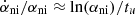${\dot{\alpha }}_{\mathrm{ni}}/{\alpha }_{\mathrm{ni}}\approx ln({\alpha }_{\mathrm{ni}})/t_u$, with t_u ≈ 14 Gyr the age of the Universe. The deceleration parameter is always close to the observed value q = −1.0 ± 0.4 (Riess et al. 1998). An interesting feature of this nonideal model is that in contrast to a ΛCDM approach that needs to introduce two parameters ρ_CDM and Λ to explain the expansion and its acceleration, we only introduce one parameter α_ni. We can therefore link the expansion to its acceleration and provide an analytical expression for q_ni, using the critical density ρ_c = 3H²/8πG. Assuming the nonideal amplification factor α_ni entirely explains the observed present-day expansion, that is, it varied from α_ni = 1 to α_ni = ρ_c/ρ_b ≈ 20 over the age of the universe, t_u ∼ 14 Gyr, we can obtain an order-of-magnitude analytical expression,

$$\begin{array}{c}\hfill q_{\mathrm{ni}}\approx \frac{1}{2}-\frac{ln({\rho }_c/{\rho }_b)}{2t_{u}H},\end{array}$$(66)

which gives a deceleration parameter q_ni = −1.06 that is compatible with the value based on type Ia supernovae (q = −1.0 ± 0.4, Riess et al. 1998).

This value contradicts current estimates using all cosmological constraints (q = −0.52 ± 0.07, Planck Collaboration VI 2020). It must be stressed, however, that the aforementioned estimates of the deceleration parameter based on the Planck results rely on the ΛCDM model. The current nonideal cosmological formalism might relax this tension: an older universe with an age of about 20 Gyr would give a nonideal deceleration parameter of about −0.5, for example. Another possibility is that the formation of structures has slowed down in the recent universe, for instance, because of feedback processes. Observations show that the cosmic star formation rate has decreased by almost a factor 10 since redshift z∼1–2, that is, within the past ∼8 − 10 Gyr (Madau & Dickinson 2014). An increase in nonideal amplification factor of about 2 within the last 7 Gyr would agree with current estimates of q. This possibility can be explored in detail with numerical simulations. Nonetheless, because the physics responsible for the acceleration of the Universe remains mysterious so far, it is quite remarkable that we can derive a good order-of-magnitude estimate of the acceleration of the expansion based on a physically intuitive and appealing argument, namely the increasing density induced by the gravitational collapse of the large-scale structures.

5. Discussion and conclusion

5.1. Nonideal Einstein equation?

As discussed in Sects. 2.2 and 2.3, we may have to step away from the traditional forms of the Poisson and Einstein equations to obtain the nonideal Friedmann equations. For a nonrelativistic fluid, the mass energy density, E_m = ρc², is dominant in the zeroth component of the stress energy tensor, T₀₀ ≈ ρc², and it would also dominate all other forms of energy, kinetic and potential: E_m ≫ E_kin, E_p, and so on. At first sight, it seems impossible for an interaction potential energy E_p to dominate the mass energy, implying that correlations in the interaction energy should not modify the Einstein equations. It must be stressed, however, that in the nonrelativistic limit of the Einstein equations, the gravitational interaction energy has a special status and should not be identified with E_p, but rather directly with the integral of T₀₀. This can be seen by deriving the Poisson equation from the Einstein equations: Δϕ ≈ −4πGT₀₀/c². The gravitational interaction energy in the nonrelativistic limit is thus given by

$$\begin{array}{cc}\hfill H_{\mathrm{int}}& =\frac{1}{2}{\displaystyle {\int }_V}\rho (\mathit{r})\varphi (\mathit{r})\mathrm{d}V\hfill \\ \hfill & \approx -\frac{1}{2}{\displaystyle \int {\int }_{V,V}}G\frac{\rho (\mathit{r})T_{00}({\mathit{r}}^{\prime })/c^2}{||\mathit{r}-{\mathit{r}}^{\prime }||}\mathrm{d}V\mathrm{d}{V}^{\prime },\hfill \end{array}$$(67)

which corresponds to the uncorrelated (ideal) version of the interaction energy. It ignores the distance between pairs of particles in the fluid because it does not depend on the correlation function. Heuristically, this explains why the contribution to the gravitational interaction energy arising from correlations should be introduced as a multiplicative factor of the mass energy (or of the gravitational constant) and not as an additional term.

Another way to show the limits of using the Einstein equation for self-gravitating correlated fluids is to consider the relativistic version of the nonideal Navier-Stokes equations introduced in Sect. 3.2: ∇_μT^μν = 0. As explained in Sect. 3.2, as soon as the Jeans length is not resolved (hence when the cosmological principle is applied at large scale), part of the gravitational interactions should be taken into account in the EOS of the fluid, hence in the definition of T^μν. The rest can be accounted for as external interactions with a mean field that can be included in the covariant derivative ∇_μ in the context of General Relativity. The gravitational interactions that contribute to the EOS cannot in general be included in the covariant derivative, which is another way to show that the equivalence principle for all the gravitational interactions is broken by the presence of correlations in a self-gravitating nonideal fluid.

We stress that the concept of nonideal self-gravity developed in the present paper does not modify the fundamental law of gravity between two point particles, which relies only on Newton’s law. Furthermore, it does not contradict Poisson and Einstein theories: they always remain valid if one can have access to or compute exactly the full inhomogeneous density distributions down to the scale below which we can assume the gas to be uncorrelated (see the example of polytropic stars in Sect. 4.1). However, for a large ensemble of particles with unresolved small-scale inhomogeneities, a nonideal modification of the Poisson and Einstein equations is required to account for the correlations between these substructures. It is worth pointing out that a modification of the Poisson equation because of correlations is a procedure already used in the case of the electrostatic force in the context of physical chemistry (see, e.g., Storey & Bazant 2012). In this field, Poisson and Einstein theories would be qualified as mean field theories, that is, they would only be valid in the uncorrelated case. A more complete theoretical approach to develop a nonideal formalism for the Einstein equations could come from two routes. Either from a homogenization procedure of the inhomogeneous Einstein equations, a path that is already currently explored (see, e.g., Buchert 2000, 2008), or from an extension of the concepts used in statistical mechanics, as developed in this paper, within a general relativistic framework.

5.2. Conclusion

Starting from the well-established BBGKY formalism, we have shown that correlations induced by bound substructures should be accounted for when describing the energy-mass density of the Universe. This should be done via the use of a nonideal virial theorem formalism and nonideal Navier-Stokes equations. When these nonideal effects are taken into account, an amplification of the gravitational interaction energy results that could account, at least partly, for the missing mass problem in galaxies, clusters of galaxies, and large-scale structures in general. The strength of this model is that the radial distribution function (or the two-point correlation function) can be well determined in galaxies and the large-scale structures either by observations or by simulations.

By examining the viscous limit of the nonideal Navier-Stokes equations induced by the presence of small-scale interactions, we showed that the presence of substructures (e.g., spiral arms and local clustering) can produce nonkeplerian rotation profiles that could explain the observed flat rotation curves. A consequence of this approach is to show that the observed bifurcation between spiral and dwarf galaxies and some LSB galaxies with Keplerian rotation profiles could be explained by the presence or absence of substructures within these galaxies. In the context of statistical mechanics, this bifurcation could be interpreted as a phase transition between two different equilibrium (viscous and nonviscous) states.

Using this nonideal virial theorem, we have derived nonideal Friedmann equations within the Newtonian limit. Using the radial distribution function of visible gas and stars obtained in large-scale simulations, we can compute the nonideal amplification factor of gravitational mass energy and show that this factor can easily be about 5 to 20 and thus could explain the observed value of the Hubble parameter. Furthermore, we show that the amplification is much stronger for the stellar component than for the gas component, which could also explain the bullet cluster observation with a high gravitational weak lensing in the stellar component compared to the gas component.

Furthermore, because most of the contribution to the value of the Hubble parameter stems from the nonideal amplification caused by the interactions between substructures, this naturally explains the acceleration of the expansion of the Universe as a consequence of the ongoing collapse, thus the increasing densities of these substructures. An amplification factor α_ni ≃ 20 during most of the lifetime of the Universe yields a deceleration parameter q_ni ≃ −1 (see Eq. (66)), close to the estimates based on type Ia supernovae. To the best of our knowledge, this model is the first that can predict a coherent value for the acceleration of the expansion of the Universe with first-principle physical arguments.

Observations of the Euclid satellite will be crucial to probe and further constrain the radial distribution function and the nonideal effects of self-gravitating matter at large scales. A precise characterization of these effects will be essential to build a full nonideal cosmological model addressing all cosmological constrains (e.g., cosmic microwave background data) and to eventually reveal what is really dark in our Universe.

Acknowledgments

We thank the anonymous referee for his/her constructive comments. We thank S. Kokh and E. Audit for co-supervising the PhD of T. Padioleau. This PhD subject is at the frontier between astrophysics and two-phase flow simulations for the cooling system of nuclear power plants and the link between liquid statistical mechanics and gravity at large scale has emerged from this trans-disciplinary approach. They also thank CEA in general (DRF and DES in particular) for the funding of the PhD and for providing a favorable environment for trans-disciplinarity at Maison de la Simulation. P.T. also thanks the Astrosim 2019 school and in particular J. Rosdhal and O. Hahn for their lectures: part of the ideas presented in this paper has emerged after the school. The authors also thank F. Sainsbury-Martinez, J. Faure, T. Buchert, G. Laibe, Q. Vigneron, P. Hennebelle, F. Bournaud, D. Elbaz, D. Borgis, R. Balian, and L. Saint-Raymond for interesting discussions and useful comments on this paper. P.T. acknowledges supports by the European Research Council under Grant Agreement ATMO 757858.

References

All Tables

All Figures

	Fig. 1. Schematic illustration of situations in which the ideal hypothesis is valid and in which it breaks down. Left: fluid is uncorrelated at all scales. Right: on the scale of control volume V1, the fluid can be considered locally as inhomogeneous and uncorrelated, while on the scale of control volume V2, the fluid can be considered as globally homogeneous and correlated.
In the text

	Fig. 2. Schematic illustrating the interactions between two fluid volumes used to derive Newton’s laws for pressureless correlated fluids.
In the text

	Fig. 3. Polytropic solutions. Top: density profiles solutions to the Lane-Emden equation with different polytropic indexes n. Bottom: total enthalpy per unit mass compared to gravitational interaction energy per unit mass assuming either a homogeneous density profile or accounting for inhomogeneities. Blue and green crosses are indistinguishable.
In the text

	Fig. 4. Snapshots of the N-body simulations from Fig. 1 in Voglis et al. (2006). The arm or spiral structures are obtained by increasing the total angular momentum from models QR1 to QR4 for the same mass and size for all the simulations.
In the text

	Fig. 5. Rotation curves of the different models from QR1 to QR4 from Fig. 2 in Harsoula & Kalapotharakos (2009).
In the text

Fig. 6. Relation between total acceleration and baryonic component for LSB and dwarf galaxies (Paolo et al. 2019). Acceleration deduced from the rotation curves of models QR1 and QR4 of Voglis et al. (2006) and Harsoula & Kalapotharakos (2009) assuming a half-mass radius of 3 kpc and a total mass of 1011 M⊙ for the galaxy. QR1 is taken as the reference for Keplerian rotation. The bifurcation between Keplerian rotation (QR1) and anomalous rotation (QR4) can be interpreted as a phase transition induced by the presence of substructures, i.e., spiral arms that have developed in model QR4.

In the text

	Fig. 7. Radial distribution function of stars and gas corresponding to the parameters given in Table 1. Case 1 corresponds to a fit of the correlation functions of the large-scale structures of the Universe at redshift 0 in the IllustrisTNG simulation from Springel et al. (2017). Case 2 uses the same stellar component, but more compact substructures in the gas component.
In the text

References

- Aslangul, C. 2006, Physique statistique des Fluides Classiques [Google Scholar]
- Balian, R., & Schaeffer, R. 1989a, A&A, 220, 1 [NASA ADS] [Google Scholar]
- Balian, R., & Schaeffer, R. 1989b, A&A, 226, 373 [NASA ADS] [Google Scholar]
- Barnes, J. E., & Hernquist, L. 1992, ARA&A, 30, 705 [Google Scholar]
- Binney, J., & Tremaine, S. 1987, Galactic Dynamics [Google Scholar]
- Bogoliubov, N. N. 1946, J. Phys.-USSR, 10, 265 [NASA ADS] [Google Scholar]
- Born, M., & Green, H. S. 1946, Proc. Roy. Soc. London Ser. A Math. Phys. Sci., 188, 10 [NASA ADS] [Google Scholar]
- Buchert, T. 2000, in Proceedings of 9th Workshop on General Relativity and Gravitation conference, 306 [Google Scholar]
- Buchert, T. 2008, Gen. Relativ. Gravit., 40, 467 [CrossRef] [Google Scholar]
- Burkert, A., & Hensler, G. 1988, A&A, 199, 131 [Google Scholar]
- Chabrier, G. 1990, J. Phys. France, 51, 1607 [NASA ADS] [CrossRef] [EDP Sciences] [Google Scholar]
- Chavanis, P. H. 2013, A&A, 556, A93 [NASA ADS] [CrossRef] [EDP Sciences] [Google Scholar]
- Davis, M., & Peebles, P. J. E. 1977, ApJS, 34, 425 [CrossRef] [Google Scholar]
- de Vega, H., & Sánchez, N. 2002, Nucl. Phys. B, 625, 409 [CrossRef] [Google Scholar]
- Hansen, J.-P., & McDonald, I. R. 2006, Theory of Simple Liquids, 3rd edn., eds. J.-P. Hansen, & I. R. McDonald (Burlington: Academic Press), 11 [CrossRef] [Google Scholar]
- Harsoula, M., & Kalapotharakos, C. 2009, MNRAS, 394, 1605 [NASA ADS] [CrossRef] [Google Scholar]
- Irving, J. H., & Kirkwood, J. G. 1950, J. Chem. Phys., 18, 817 [NASA ADS] [CrossRef] [Google Scholar]
- Kirkwood, J. G. 1946, J. Chem. Phys., 14, 180 [NASA ADS] [CrossRef] [Google Scholar]
- Kirkwood, J. G., Buff, F. P., & Green, M. S. 1949, J. Chem. Phys., 17, 988 [NASA ADS] [CrossRef] [Google Scholar]
- Li, C., & White, S. D. M. 2009, MNRAS, 398, 2177 [NASA ADS] [CrossRef] [Google Scholar]
- Madau, P., & Dickinson, M. 2014, ARA&A, 52, 415 [Google Scholar]
- Markevitch, M., Gonzalez, A. H., Clowe, D., et al. 2004, ApJ, 606, 819 [NASA ADS] [CrossRef] [Google Scholar]
- Paolo, C. D., Salucci, P., & Fontaine, J. P. 2019, ApJ, 873, 106 [NASA ADS] [CrossRef] [Google Scholar]
- Peacock, J. 1999, Cosmological Physics, Cambridge Astrophysics (Cambridge University Press) [Google Scholar]
- Peebles, P. J. E. 1980, The Large-Scale Structure of the Universe [Google Scholar]
- Pfenniger, D. 2006, Comp. Ren. Phys., 7, 360 [NASA ADS] [CrossRef] [Google Scholar]
- Planck Collaboration VI. 2020, A&A, 641, A6 [NASA ADS] [CrossRef] [EDP Sciences] [Google Scholar]
- Riess, A. G., Filippenko, A. V., Challis, P., et al. 1998, AJ, 116, 1009 [Google Scholar]
- Springel, V., Pakmor, R., Pillepich, A., et al. 2017, MNRAS, 475, 676 [Google Scholar]
- Storey, B. D., & Bazant, M. Z. 2012, Phys. Rev. E, 86, 056303 [NASA ADS] [CrossRef] [Google Scholar]
- Truelove, J. K., Klein, R. I., McKee, C. F., et al. 1997, ApJ, 489, L179 [CrossRef] [Google Scholar]
- Voglis, N., Stavropoulos, I., & Kalapotharakos, C. 2006, MNRAS, 372, 901 [NASA ADS] [CrossRef] [Google Scholar]
- Whitaker, S. 1998, The Method of Volume Averaging, Theory and Applications of Transport in Porous Media (Netherlands: Springer) [Google Scholar]
- Yvon, J. 1935, La théorie statistique des fluides et l’équation d’état, Actualités Scientifiques et Industrielles: Théories Mécaniques (Hermann& cie) [Google Scholar]
All Tables
Parameters used to parameterize the radial distribution function of gas and stars for case 1 and case 2.
Nonideal amplification of the different component (gas-gas, star-star, and gas-star) for two different values of the threshold gth used to define the bound radius.