| Issue |
A&A
Volume 662, June 2022
|
|
|---|---|---|
| Article Number | A82 | |
| Number of page(s) | 15 | |
| Section | Catalogs and data | |
| DOI | https://doi.org/10.1051/0004-6361/202141926 | |
| Published online | 22 June 2022 | |
Detection of period-spacing patterns due to the gravity modes of rotating dwarfs in the TESS southern continuous viewing zone★
1
Instituut voor Sterrenkunde (IvS), KU Leuven,
Celestijnenlaan 200D,
3001
Leuven,
Belgium
e-mail: This email address is being protected from spambots. You need JavaScript enabled to view it.
2
Department of Astrophysics, IMAPP, Radboud University Nijmegen,
PO Box 9010,
6500
GL Nijmegen,
The Netherlands
3
Max Planck Institute for Astronomy,
Koenigstuhl 17,
69117
Heidelberg,
Germany
Received:
1
August
2021
Accepted:
22
November
2021
Abstract
Context. The theory of stellar evolution presents shortcomings when confronted with asteroseismic probes of interior physical properties. The differences between observations and theory are often great because stellar models have mainly been calibrated from observables connected to the surface of stars. Period-spacing patterns caused by gravity modes are a particularly powerful asteroseismic tool that are useful for probing the near-core rotation and mixing of chemical elements in main-sequence stars with convective cores.
Aims. We aim to compose a catalog of intermediate-mass stars in the Transiting Exoplanet Survey Satellite (TESS) southern continuous viewing zone (CVZ) to reveal period-spacing patterns caused by gravity modes for use in future asteroseismic modeling.
Methods. TESS full frame images (FFI) were inspected to select stars of intermediate- and high-mass using color-magnitude criteria. Light curves were extracted from custom masks per star, adopting stringent constraints on the aperture masks and contamination. The extracted light curves were subject to iterative prewhitening to detect gravity modes. We developed a method relying on the assumption that period spacings are an approximately linear function of the mode periods to build a template pattern. This template was used to extract the patterns and their uncertainties, relying on a bootstrap approach.
Results. Our TESS catalog of high-quality period-spacing patterns is the first of its kind and contains 140 gravity-mode patterns in 106 γ Dor stars and two slowly pulsating B-type (SPB) stars. Half of these patterns contain seven or more measured mode periods and the longest pattern contains 20 modes. We provide the community with a convenient software tool to search for period-spacing patterns and to process the extracted light curves.
Conclusions. Our catalog offers a fruitful starting point for future gravity-mode asteroseismology of rotating dwarfs with convective cores in the southern hemisphere.
Key words: asteroseismology / catalogs / stars: interiors / stars: rotation / stars: variables: general
The catalog file of stars with period-spacing patterns is available in electronic form at the CDS via anonymous ftp to cdsarc.u-strasbg.fr (130.79.128.5) or via http://cdsarc.u-strasbg.fr/viz-bin/cat/J/A+A/662/A82. The supplementary material, that presents the period-spacing pattern in our catalog, is available at https://doi.org/10.5281/zenodo.6320990
© ESO 2022
1 Introduction
The theory of stellar structure and evolution is well established and capable of describing the different stages of a star throughout its life in general terms (e.g., Kippenhahn et al. 2012). However, the theory is mostly calibrated to the surface properties of stars, such as their surface gravities, surface chemical compositions, surface rotations, and effective temperatures. Today, advances in asteroseismology and the advent of high-precision space photometry from telescopes such as CoRoT (Auvergne et al. 2009), Kepler (Koch et al. 2010) and TESS (Ricker et al. 2015) allow us to probe stellar interiors with a precision that cannot be reached from extrapolating surface quantities (e.g., Hekker & Christensen-Dalsgaard 2017; García & Ballot 2019; Bowman 2020; Aerts 2021, for recent reviews). Asteroseismic modeling based on space photometry has revealed large discrepancies between observations and the theory of stellar structure and evolution, such as in the transport of angular momentum (e.g., Aerts et al. 2019).
Gravity modes (hereafter g modes) are stellar oscillations that have buoyancy as their dominant restoring force and have optimal probing power in the near-core regions of main-sequence stars (e.g., Aerts et al. 2018). They are detected in main-sequence stars with a convective core and a radiative envelope known as γ Doradus (γ Dor) stars (Kaye et al. 1999) and SPB stars (Waelkens 1991), which have masses from 1.3 to 1.9 M⊙ and 3 to 9 M⊙, respectively (e.g., Aerts et al. 2010, Chapter 2, for more properties). To detect and accurately measure the frequencies of their individual g modes, which have periodicities of the order of days, high-precision long-term uninterrupted observations are needed. These requirements are met for time-series photometry from space missions such as Kepler and TESS, which allows us to detect g-mode period spacing patterns. The first such detection in a dwarf was made for the SPB star HD 50230 from CoRoT space photometry by Degroote et al. (2010). The five-month CoRoT light curve was sufficient to detect a period-spacing pattern of eight dipole g modes thanks to this star’s very slow rotation, also justifying asteroseismic modeling having ignored the Coriolis acceleration in the pulsation computations (Wu & Li 2019).
Gravity-mode period-spacing patterns, describing the difference in periods of g modes with an identical spherical degree, ℓ, and azimuthal order, m, while having a consecutive radial order, n, are a powerful asteroseismic tool (Aerts et al. 2010, for a detailed theoretical derivation). This tool allows us to probe the near-core regions of main-sequence stars with convective core and a radiative envelope. As shown by Shibahashi (1979) and Tassoul (1980), g-mode periods, Pnℓ, are equidistant for a spherical chemically homogeneous non-rotating star when considering the asymptotic regime, that is, with 2π/Pnℓ ≪ N with N the buoyancy frequency:
 (1)
(1)
with
 (2)
(2)
where ϵg is a phase term which depends on the boundaries, r1 and r2, of the g-mode propagation cavity. Gradients in the stellar chemical composition profile cause mode trapping, which introduces wave-like behavior and periodic dips also known as buoyancy glitches in the period-spacing patterns. As shown by Miglio et al. (2008), the amplitude and location of these modulations in the pattern depend on the steepness and the location of the chemical gradients inside the star.
For a rotating star, the Coriolis acceleration and the difference between the corotating reference frames and the inertial ones of the observer shift the g-mode frequencies quite drastically. As a result, the observed period spacings reveal a decreasing trend for prograde (m > 0) and zonal (m = 0) modes when plotted as a function of increasing mode period as observed in an inertial frame of reference. For retrograde modes (m < 0), on the other hand, an overall increase in the observed spacings of modes with increasing pulsation period occurs (e.g., Bouabid et al. 2013; Van Reeth et al. 2015a,b; Ouazzani et al. 2017). Schmid & Aerts (2016) investigated the limit of the rotation frequency at which the Coriolis acceleration can still be treated perturbatively and found this approximation already breaks down for rotation frequencies above roughly ~ 0.1 d−1, which is the case for almost all intermediate-mass dwarfs (cf. Aerts et al. 2017).
A strong magnetic field in the stellar interior requires the Lorentz force to be included in the pulsation computations. This modifies the morphology of the observed period spacing pattern by introducing a saw-tooth modulation of the period spacing values as the consecutive pulsation periods increase (Prat et al. 2019, 2020; Van Beeck et al. 2020). Moreover, coupling between inertial modes in the rotating core and g modes in the envelope occurs and may cause dips superposed to buoyancy glitches at particular mode periods in the spacing diagram (Ouazzani et al. 2020; Saio et al. 2021; Lee 2021). This implies that interpretations of buoyancy glitches from mathematical analytical descriptions ignoring the Coriolis acceleration (e.g., Cunha et al. 2019) can only be applied to slowly-rotating non-magnetic stars. The majority of g-mode pulsators require the modeling and interpretation of the observed period spacing patterns to be done numerically, based on the inclusion of the Coriolis (and perhaps Lorentz) force when solving the pulsation equations (cf. Townsend & Teitler 2013; Townsend et al. 2018).
After the initial discovery by Degroote et al. (2010), it took another five years before period-spacing patterns were detected from four-year Kepler light curves in several hundreds of γ Dor stars (e.g., Van Reeth et al. 2015b; Li et al. 2019, 2020) and several dozens of SPB stars (e.g., Pápics et al. 2017; Pedersen et al. 2021; Szewczuk et al. 2021). These patterns have been used to measure the near-core rotation rates of all these stars (e.g., Van Reeth et al. 2016, 2018; Christophe et al. 2018; Li et al. 2019, Li et al. 2020; Takata et al. 2020; Pedersen et al. 2021) and place constraints on the chemical transport processes that take place in the deep stellar interior (e.g., Mombarg et al. 2020, 2021; Pedersen et al. 2021). From the point of view of improving stellar evolution theory, dwarfs are the most interesting targets as they still have their evolved stages ahead of them and uncertainties in the transport processes are cumulative over time. Moreover, g modes are potentially excited along the main sequence in various instability regions for stars born with a convective core covering a broad mass range (Aerts et al. 2010, Chapter 3). This is why we focus our work on dwarfs covering spectral types between O and F.
To date, the photometric observations obtained with the nominal Kepler mission cover the longest time base and are more precise than the observations from any other high-cadence space-photometry mission. Hence, most breakthroughs in g-mode asteroseismology of dwarfs were achieved thanks to Kepler observations so far. Here, we exploit the asteroseismic potential of the ongoing TESS space mission and compare it to that of Kepler. The TESS extended mission is gradually providing data of progressively higher frequency resolution and has opened the door to analyzing numerous stars located in regions of the sky other than the Kepler field of view and in different metallicity regimes. In this work, we present results based on the first full year of uninterrupted TESS monitoring, to evaluate its capacity for the g-mode asteroseismology of rotating dwarfs. Future works will involve the addition of data from the extended TESS mission to the stars in our current catalog to increase their capacity for asteroseismic modeling.
Our study is aimed at identifying new γ Dor or SPB stars that have been observed by TESS in the southern continuous viewing zone (CVZ) to build the first TESS catalog of high-quality g-mode period-spacing patterns for such pulsators. The southern CVZ was observed uninterruptedly during the first year of the nominal TESS mission, with a 24° square field-of-view centered at the Southern ecliptic pole rotating about every 27 d. This long observation period has provided light curves with a nominal frequency resolution of about 0.003 d−1.
The paper is organized as follows. In Sect. 2, we describe our criteria for selecting O/B- and A/F-type stars in the TESS southern CVZ. In Sect. 3, we describe our method used to extract light curves from the TESS full frame images, including our data analysis treatments to detrend and optimize the extracted light curves to search for g modes. In Sect. 4, we discuss the frequency extraction from the light curves and our posterior analysis. Section 5 describes our method for finding period-spacing patterns. Finally, we discuss our final catalog of g-mode pulsators with period-spacing patterns in Sect. 6.
2 Data set
To select our sample of stars, we started from the TESS Input Catalog (TIC) version 8 (Stassun et al. 2019) and reduced it to the TESS southern CVZ by imposing an ecliptic latitude β ≤ −72°. To exclude extended objects and keep only point-like sources, we used the TIC’s flag Objtype=star. Stars likely to be white dwarfs or giants were identified with the TIC’s flag wdflag=1 and lumclass=GIANT, respectively, and excluded from the sample. The first flag represents a cut in absolute Gaia magnitude and Gaia color (GBP − GRP) while the second flag represents a cut in radius (calculated from Gaia parallaxes) and Teff. We refer to Stassun et al. (2019) for a description of the TIC flags.
To narrow down our sample of stars to candidates of spectral type F and hotter, that is the most likely g-mode pulsators, we used 139 TESS O/B-type stars selected manually by Pedersen et al. (2019) and 616 Kepler A/F-type γ Dor pulsators taken from Tkachenko et al. (2013); Li et al. (2020). We placed those stars in a color-magnitude diagram and used them to define two pairs of color-magnitude cuts that enclose 95% of these bona fide O/B- and A/F-type stars. By applying these pairs of cuts to our TESS sample, we extracted all the O/B- and A/F-type candidate pulsators of interest. We calculated their absolute magnitudes as
 (3)
(3)
where m is the apparent magnitude in a given passband. To obtain the distance d, we used the Bayesian distance estimate from Bailer-Jones et al. (2018) reported in the TIC. To ensure reliable distances, we used stars with a positive Gaia parallax of relative error of less than 25% that passed both astrometric and photometric criteria given by Eqs. (1) and (2) in Arenou et al. (2018), namely, with TIC flag gaiaqflag=1. To minimize the effect of extinction, we used the 2MASS infrared bands J, H, and K and adopted the cuts listed in Table 1. Figure 1 shows these cuts in K and J–K as straight lines and our sample in the background. A/F-type candidates correspond to stars in the top-left quadrant delineated by the red straight lines minus the O/B-type candidates that correspond to stars in the top-left quadrant delineated by the cyan straight lines. The final candidates are obtained after an analogous additional selection in a color-magnitude diagram based on H and J – H. Table 1 and Fig. 1 do not consider corrections for extinction. The potential contamination by cooler stars that are not expected to pulsate in g modes will be treated in Sect. 4, based on the frequency analysis results.
Finally, to favor a high signal-to-noise ratio (S/N) and non-contaminated flux in the light curves, we limited our sample further to stars with apparent TESS magnitude brighter than 15 (uncorrected for extinction) and situated at least 2 arcsec apart from other stars in the TIC. Our selected sample consists of 345 O/B-type candidates and 9369 A/F-type candidates in the TESS southern CVZ, all from our Galaxy.
Cuts used to define O/B- and A/F-type candidates.
3 Our TESS data reduction pipeline
We searched sectors 1–13 of TESS for long-cadence (i.e., 27.4 min) full-frame images available in the Mikulski Archive for Space Telescopes and used the TESScut API (Brasseur et al. 2019) to download, for every star in our sample, a 20 × 20 pixel image with the target star at the center. These images are known as target pixel files and contain the flux information for all available time stamps. The 20 × 20 pixel size was chosen such that the target pixel file contains both the flux of the target star and the flux of the representative background around it; a typical example is shown in Fig. 2 in which the middle panel shows a background mask 11 times larger than the aperture mask. Light curves were extracted from the target pixel files using aperture photometry, as explained in Sect. 3.1, while the background and systematic effects were corrected using two standard statistical methods, that is, a principal component analysis (PCA) and a linear regression, as further detailed in Sect. 3.2. The Python package Lightkurve (Lightkurve Collaboration 2018) was used during the reduction.
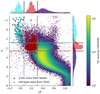 |
Fig. 1 2MASS color-magnitude diagram showing the pairs of cuts in absolute magnitude and color defining candidate g-mode pulsators of spectral type O/B (cyan straight lines) and A/F (red straight lines) in K and J–K. The cyan and red circles are bona fide O/B- and A/F-type stars, respectively, while the retained dwarfs from the TIC in the southern CVZ are plotted in the background. The side histograms show the distribution of stars; the pairs of cuts enclose 95% of the respective bona fide stars. |
3.1 Aperture and background masks
To define the aperture mask of a star, we used the median frame of all the target pixel files (left panel in Fig. 2) and selected all pixels with a flux count larger than the median flux plus n-times the standard deviation. Those pixels are our first estimate of the aperture mask. The standard deviation was robustly estimated as 1.4826 times the median absolute deviation (Ruppert 2011). To reduce the contamination from nearby stars falling into the aperture mask, we used the increasing values of n = 5.0, 7.5, 10, 15, 20, 30, and 40 for the threshold in standard deviation to shrink the aperture mask until the target star was the only bright star contained within it by at least 4 TESS magnitudes. The target and neighboring stars with apparent TESS magnitudes  and mTESS, respectively, within the aperture mask thus follow the condition:
 (4)
(4)
ensuring that the flux of individual fainter stars contributes no more than approximately 0.25% of the total flux within the aperture mask. For cases where the resulting aperture mask consists of disjointed sets of pixels, only the set containing the target star is kept. Finally, to help prevent flux from neighboring stars leaking into the aperture mask, pixels showing an increase in flux in any direction away from the target star are removed from the mask and used as its edge. The background mask was defined in the same way as the first estimate of the aperture mask but selecting the pixels below a threshold with n = 3, thus ensuring a minimum two-standard-deviation flux gap between the aperture mask and the background mask. A typical example of both final apertures is shown in the middle panel of Fig. 2.
To estimate the level of contamination in the aperture mask due to the flux of neighboring stars, we calculate the ratio of this flux to that of the target star. To obtain such fluxes, all stars complying with Eq. (4) were modeled as 2D Gaussian functions and fitted to the median image of the target pixel file along with a 2D plane to account for the background flux. The Gaussian functions were centered at the location of each star, had all the same standard deviation, and their relative amplitudes kept the same relation as the fluxes from the stars. Fluxes were converted from TESS magnitudes using the TASOC Photometry pipeline (Handberg et al. 2021). The right panel in Fig. 2 shows an example of this fit.
We rejected the aperture mask (together with the target pixel file) when the final mask contained stars that do not comply with Eq. (4). To avoid both corrupted and bleeding pixels, we also rejected masks that had pixels with null counts or that were too elongated (i.e., with fewer than four rows or columns, while the other is at least 14-pixels long). To average out the stochastic noise of individual pixels, we only kept aperture masks with at least nine pixels, as shown in the left panel of Fig. 3. After careful assessment, our sample consisted of 2162 stars with a flux contamination due to neighboring stars smaller than 5%, as shown in the right panel in Fig. 3. The middle panel in Fig. 3 shows that our light curve extraction is consistent with previous data pipelines for which the extraction is considered to be trustworthy only for stars brighter than TESS magnitude of 13.5 (e.g., Handberg et al. 2019; Huang 2020; Caldwell et al. 2020).
Because of our stringent constraints on the aperture mask, not all TESS sectors yielded a satisfactory mask for a given star. We therefore only kept stars with aperture masks found in at least 11 of the 13 TESS sectors, as shown by the dashed line in Fig. 4. The 11 sectors are not necessarily consecutive. After this cut, our sample consists of 1967 stars. Figure4 also shows a higher level of contamination when the aperture mask is found in fewer numbers of TESS sectors, indicating that stars in a crowded field are more prone to fail the requirements of the aperture mask selection.
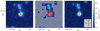 |
Fig. 2 Square 20-by-20 pixels around TIC 38845463, TESS sector 1. The color bar is common to the three panels and shows a logarithmic scale of the flux in electrons per second. The red circle represents the target star while white circles indicate TIC neighboring stars down to four TESS magnitudes fainter with respect to the target star. The symbol sizes are inversely proportional to the TESS magnitude. Declination grids are 2′ apart. Left: median image of the target pixel file. Middle: panel with the final aperture mask (red shade) and background mask (gray shade) overplotted. The aperture mask results from the threshold parameter n = 20 (see text for explanation). Right: best fit based on the left panel used to estimate the level of contamination in the aperture mask due to flux from neighboring stars. The image was modeled as six 2D Gaussian functions plus a 2D plane. See Sect. 3.1 for further details. |
 |
Fig. 3 Our star sample without constraints on the aperture mask size (7385 sources, gray histogram) and after imposing a minimum size of 9 pixels (2162 sources, blue histogram). Other constraints described in Sect. 3.1 apply to both histograms. Left: sample distribution of the median aperture mask sizes, calculated per star over all TESS sectors. Middle: sample distribution of the TESS magnitudes. The dashed red line marks a magnitude value of 13.5. Right: median contamination level caused by neighboring stars, calculated per star over all TESS sectors. The dashed orange line marks a contamination of 5%. |
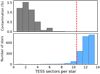 |
Fig. 4 Blue histogram in the bottom shows the number of TESS sectors per star with a satisfactory aperture mask. The dark-gray histogram shows the mean contamination in each bin of the blue histogram. The dashed red line shows the cut for stars with at least 11 TESS sectors (a total of 1967 stars). |
3.2 Light curve extraction and correction
To remove part of the systematic flux variability in the extracted light curves, we used the data quality flags provided in the headers of the target pixel file1 (Twicken et al. 2020) and removed the data from the time stamps affected by loss of fine pointing2, thermal transients3, Earth pointing, and other specific effects4 (e.g., coronal mass ejections). We then extracted the light curves using simple aperture photometry with the aperture masks we constructed as described in Sect. 3.1. An example is shown in Fig. 5, where the gaps in the data correspond to the removed time stamps. We noted that the use of the quality flags according to the TESS release notes did not cover all systemics present in the light curves and proceeded to manually remove time intervals (common to all stars) which still were significantly affected by systematic effects (e.g., telescope jittering, thermal transients, and loss of fine pointing). Such time intervals are present in sectors 1 to 8, as listed in Table A.1 and shown in red in Fig. 5.
The remaining systematic variability (e.g., the gradual increase of flux in sector 2 due to scattered light or the rapid decrease of flux at the beginning of sector 8 as illustrated in Fig. 5) and background flux were removed using a linear regression of the light curve against the flux variability present in the background mask defined in Sect. 3.1. We started this process by extracting a light curve using aperture photometry from each of the background pixels (an average of 330 pixels per pixel target file in our sample). Subsequently, we applied a PCA to these light curves to capture their dominant flux variability (see Feinstein et al. 2019). We let B be the matrix whose columns are the light curves extracted from the background pixels, its singular value decomposition is
 (5)
(5)
where U and V are orthonormal matrices and S is a diagonal matrix with entries si > si+1. The principal components of B are given by the columns of US, which are ordered by their contribution to the background flux variability. No universal number k of principle components can be used to estimate background flux variability because different TESS sectors are subjected to different systematic effects. Since the first principal components capture most of the systematic variability while subsequent ones are affected by an increasing amount of white noise (see Fig. 6 for an example), we used the level of scatter in the normalized principal component (columns of U) as a criterion to determine k. The level of scatter was determined by the median of the moving variances with a window length W = 16 h. Denoting the elements in a column of U by f(t), where the time t represents a cadence, the moving variance at a cadence t was computed as
 (6)
(6)
where  is the mean of f(tn) within the window |tn − t| < W. The W = 16 h was chosen to yield a large number of short light curve segments while being shorter than the typical period of g modes. We found that the level of scatter in the columns of U, that is, ui, increased with i as expected, since increasing values of i had less systematic signal and more white noise. The level of scatter converged to a value of order 10−3 for i ≳ 6 regardless of the TESS sector. We therefore used the principal components with a level of scatter <10−4 to represent the systematic variability present in the background. The median number of principal components used by our method is k = 4. To prevent further injection of white noise into the reduced light curves, we used a maximum of seven principal components.
Once the number k of principal components was determined, we created the regressor matrix X, using the principal components as its columns and added a constant column to account for a constant level of background. Subsequently, we performed the following linear regression, assuming that the model fits the data within Gaussian uncertainties:
 (7)
(7)
where Y represents the uncorrected light curve of the target star, w contains the regression coefficients, and ε represents the noise. The corrected light curve was then computed as Y − Xw. These corrected light curves were then normalized by subtracting their mean flux and then dividing them by it. Values further away than 5σ were treated as outliers and removed (e.g., spikes due to cosmic rays). Finally, we stitched together the normalized light curves from each TESS sector as shown in Fig. 7.
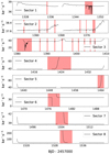 |
Fig. 5 Uncorrected light curves of TIC 30192406, showing in red the time intervals that have been excluded for all stars according to Table A.1. Sector 1 shows an example of jittering of the satellite. Sector 2 shows an example of scattered sunlight reflected by the Earth or the Moon. Sector 3 shows an example of systematic flux variability caused by the periodic re-pointing of the camera. |
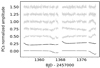 |
Fig. 6 First seven normalized principal components (PC; columns of the matrix U) from the background mask of TIC 374944608, sector 2. The PCs are displayed in ascending order with the first normalized PC at the bottom and manually set 0.25 units apart from each other for a better visualization. Only black normalized PCs have a level of scattering <10−4 (see Sect. 3.2) and were used for the detrending of the light curve. |
4 Frequency analysis from iterative prewhitening
We analyzed the light curves resulting from our developed data analysis pipeline following a procedure of iterative prewhitening. Van Beeck et al. (2021) has offered an extensive description of five different prewhitening methods applied to g-mode pulsators, relying on various regression techniques and stopping criteria. Since Van Beeck et al. (2021) developed their methodology for g modes in SPB stars and four-year Kepler light curves, their paper is highly relevant for our TESS work as well. We refer to that paper for a detailed description, as well as an elaborate comparative study of the efficiency of these five methods. Here, we rely on a method using the same frequency resolution restriction, a stopping criterion based on the amplitudes of the modes, and a nonlinear optimization to achieve the final regression result, as such methods were found to be the most powerful procedures based on the assumption of a harmonic fit to the light curve by Van Beeck et al. (2021, see methods 2 and 3). We provide a summary of the adopted procedure, where frequencies were extracted in a 5-step process from the stitched light curves as the one shown in Fig. 7.
Step 1: We computed a Lomb-Scargle periodogram of the light curve using a 10-fold oversampled frequency range (compared to T−1 with T the time span of the light curve) from zero up to the Nyquist frequency. The frequency with highest amplitude is selected and a harmonic fit with that frequency to the light curve is determined, using linear regression. The best-fitting harmonic function is subtracted from the light curve and the process is iteratively repeated on the residual light curve until the selected frequency has an amplitude with S/N < 4. The noise level is calculated as the mean amplitude of the periodogram within a symmetric frequency window of size 1 d−1 centered on the selected frequency. In order to find candidates with g-mode period-spacing patterns, we only kept stars with at least ten significant potential g-mode frequencies, that is, those with pulsations of periods longer than 0.25 days. This restriction, illustrated in Fig. 8, leaves us with a sample of 369 candidate stars.
Step 2: Unresolved frequencies were removed by requiring a conservative difference of at least 2.5 × T−1 between extracted frequencies (Loumos & Deeming 1978). In case of unresolved frequencies, we kept the one with the largest amplitude.
Step 3: All accepted frequencies were optimized simultaneously using a Levenberg-Marquardt algorithm to perform a non-linear regression, with the output of the linear regression as initial input guesses. Uncertainties in the parameters were calculated following Montgomery & O’Donoghue (1999) and corrected for their possible correlated nature following Schwarzenberg-Czerny (2003). Frequencies whose corresponding amplitudes were consistent with zero within three standard deviations were considered as insignificant and rejected.
Step 4: To minimize the influence of the spectral window convolved with dominant frequencies in the periodogram during the iterative prewhitening process, we used the amplitude criterion developed by Van Reeth et al. (2015a):
 (8)
(8)
where Af and Aloc are the optimized amplitudes and the amplitudes from the original Lomb-Scargle periodogram, respectively. This constraint is independent of the S/N and helps to avoid spurious frequency detections that can occur for space time-series data like Kepler and TESS with S/N > 4 (e.g., Zong et al. 2016; Baran & Koen 2021; Bowman & Michielsen 2021). Moreover, Van Beeck et al. (2021) have shown criteria based on mode amplitudes to work better than just using S/N as a stop criterion. In practice, we used α = 0.75, which was found to work optimally for TESS light curves by Antoci et al. (2019).
Step 5: Combination frequencies were not considered as independent mode frequencies to hunt for period-spacing patterns. Such combination frequencies were identified through the following equation:
 (9)
(9)
where we adopt the terminology of Degroote et al. (2009), meaning that fi and fj are the parent frequencies, ni and nj are integer combination coefficients, fk is the combination frequency, and ε is the threshold tolerance. We selected the 20 highest-amplitude frequencies per star as parent frequencies and searched for combinations of up to two parents, which leads to |ni| + |nj| ≤ 2.
Given the large number of frequencies per star (we note that Fig. 8 only counts g modes and ignores p modes), a linear combination of frequencies is likely to occur close to another independent frequency in the data without having to be a combination frequency (Pápics 2012; Kurtz et al. 2015). This is illustrated in Fig. 9 by the background count level marked with a gray shade while genuine combination frequencies correspond to the excess above such level. We therefore took three times that background level (gray dashed line in Fig. 9) as a 67% probability of being a genuine combination frequency. Such a probability corresponds to ε = 0.0002 (red vertical line in Fig. 9) and is consistent with the threshold tolerance reported by Li et al. (2019).
Figure 10 shows the impact on the number of independent mode frequencies after each step of the frequency analysis. As an example, the final accepted frequencies of TIC 374944608 (light curve in Fig. 7) are indicated with vertical dotted lines in Fig. 11 (to be discussed below). We checked the 369 light curves of our sample after the frequency analysis and removed eclipsing binaries. These were studied further in the separate paper by IJspeert et al. (2021). We also inspected the light curves for cases where systematic flux variability persisted after our data reduction pipeline (see Sect. 3) and removed these from the sample. This inspection was done by eye, narrowing down our sample of period-spacing pattern candidates to 304 stars.
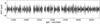 |
Fig. 7 Final light curve for TIC 374944608 as derived from our developed pipeline discussed in Sect. 3. |
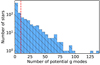 |
Fig. 8 Number of potential g-mode pulsations with S/N ≥ 4 per star. Frequencies were deduced from Step 1 described in Sect. 4. Our sample of 1967 stars has 1108 stars that are not in compliance with our Step 1 criterion and those are not plotted. The dashed red line shows the cut used to select rich enough period-spacing pattern candidates, namely, stars with at least ten significant mode periods. This resulted in 369 candidate pulsators. |
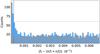 |
Fig. 9 Histogram following Eq. (9) for the frequencies of stars in our g-mode sample. The gray shade marks the background level that represents a random match among combination frequencies and the horizontal dashed gray line marks 3 times that level. The vertical red shows the intercept of the dashed gray line and the distribution; it marks ε = 0.0002 according to Eq. (9). Frequencies occurring to the left of this line have a 67% probability of corresponding to a genuine combination frequency. |
5 Period-spacing pattern search
To search for period-spacing patterns in our sample, we fitted the following template to the list of periods of each star (Li et al. 2019):
 (10)
(10)
where ΔPj = Pj+1 − pj is the local period spacing and Δp0 is the period spacing at a reference period p0. This period pattern allows for a linear change α ≡ d(Δp)/dp of the local period spacing caused by stellar rotation (Ouazzani et al. 2017; Christophe et al. 2018; Li et al. 2019). The template depends on the three parameters {p0, Δp0, α}. To account for the amplitude of the individual periods and the local size of the period spacing, we fitted Eq. (10) to the observations, by minimizing the following custom cost function:
 (11)
(11)
where Pi is the estimated period closest to the observed pulsation period  , ΔPi is the estimated local period spacing, Ai is the observed amplitude corresponding to
  , Amax is the maximum observed amplitude, and σi is the observed period uncertainty. Rather than minimizing the square of the absolute differences
  , we minimize the relative differences
  . In this way, period mismatches are more strongly penalized when they are large compared to the local period spacing. The addition of
  in the denominator serves to limit the penalization when the local period spacing is comparable to the observational period uncertainty, σi. The extra weight, Ai/Amax, serves to penalize a pattern more strongly when it mismatches the higher-amplitude mode periods. The minimization of the cost function S was done with the quasi-Newton method L-BFGS-B (Byrd et al. 1995) implemented in the Python module Scipy (Virtanen et al. 2020).
To find the location of the patterns in the periodogram as well as the initial guesses  for the fit, we used two diagnostic plots to cover both the cases of rapid and slow rotators. Slow rotators show an approximately constant period spacing. Their period-spacing pattern can therefore be identified in an échelle diagram, where the period is plotted as a function of the period modulo ΔP. In such a case, g modes of a given angular degree roughly form vertical ridges (analogous to the acoustic modes in the case of solar-like oscillations). On the other hand, rapid rotators show a period spacing that depends approximately linearly on the mode period (Van Reeth et al. 2016; Ouazzani et al. 2017). Therefore, their period-spacing pattern can be easier identified in a plot of ΔP as a function of period. For each star, we also complemented such two plots with a periodogram where observed and template periods were overplotted.
To facilitate the exploration of the parameter space, we developed the interactive tool FLOSSY5, a Python utility that allows a user to efficiently browse the periodogram of a large number of stars and visualize the period-spacing patterns by displaying the period échelle diagram and period-spacing plot at each location in the periodogram. FLOSSY also overplots Eq. (10) in the aforementioned plots with customized parameters {P0, ΔP0, α}. The latter can be modified on the fly, along with the number of mode periods to fit. Figure 11 shows part of FLOSSY’s output, as well as the best-fit pattern for TIC 374944608.
We used FLOSSY to manually select the θinit for every candidate period-spacing pattern found from the list of mode periods per star. In doing so we considered the parameter space  , 100 s ≤ ΔP0 ≤ 4000 s and, −0.3 ≤ α ≤ 0.3, where
  and δP corresponds to the resolution set in Step 2 of the procedure discussed in Sect. 4. To ensure that we found a global minimum, we computed S around the best-fit solution in a radius of 400 s for P0, 40 s for ΔP0, and 0.05 units for α. Those values for S are shown in Fig. 12, which is also an output of FLOSSY.
To estimate uncertainties for the detected period-spacing pattern, we computed the 68% confidence interval of the parameters using a bootstrap method with non-parametric residual resampling in the periodogram. We generated 10 000 datasets of the same size as the original one. Subsequently, we minimized Eq. (11) in each of these datasets using as initial guess the same θinit as in the original best fit. The confidence intervals were then determined as the 16% and 84% quantiles of the bootstrap distribution for the parameters θ. As an example, Fig. 13 shows the bootstrap distribution of α for the pattern found in TIC 374944608.
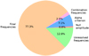 |
Fig. 10 Number of frequencies remaining in our sample after each step in Sect. 4 is applied. The pie chart is based on the frequencies of the 369 stars after step 1 of our frequency analysis. The total number of frequencies is 10927. |
6 Catalog of g-mode pulsators in the TESS southern CVZ with identified period-spacing patterns
Our final catalog of g-mode pulsators revealing period-spacing patterns consists of 108 bright dwarfs in the TESS southern CVZ. These stars revealed a total of 140 resolved period-spacing patterns. Each of these patterns are shown in the supplementary material in the same format as Figs. 11 and 12. Stars in our catalog have apparent TESS magnitudes between 7.5 and 12, with a median of about 10; the star TIC 350144657 is an exception with an apparent TESS magnitude of about 6.9. The contamination of light curves, due to the flux from neighboring stars, is < 2% thanks to our stringent requirements on the aperture mask described in Sect. 3.1. Figure 14 shows the distributions of brightness and contamination in the catalog. Only two stars, TIC 177162802 and TIC 375038081, are candidates to be SPB stars, as determined by the color-magnitude selection done in Sect. 2, while the other members of the catalog are γ Dor stars. Figure 15 shows a Gaia color-magnitude diagram that compares our catalog to the 611 γ Dor stars with detected period-spacing patterns found by Li et al. (2020) in 4-yr Kepler light curves. We find that our catalog stars appear to occur on the hotter end of the Kepler γ Dor stars because of the uncorrected reddening (T. R. Bedding, priv. comm.).
Out of the 140 period-spacing patterns, 93 have a downward slope (α < 0) and 47 have an upward slope (α > 0). The former are prograde or zonal g modes while the latter are retrograde g modes or Rossby modes (Van Reeth et al. 2016). The averaged period-spacing value per pattern, 〈ΔP〉, is ~110 s. The shortest pattern contains four measured pulsation periods, more than half of the patterns contain more than 12 and the longest pattern contains 20. In 26% of the stars we detected two or three patterns. When multiple patterns are detected in a star, this allows for a better constraint of the stellar interior from asteroseismic modeling (Aerts et al. 2018). Furthermore, 29% of our catalog stars are hybrid pulsators, meaning that they also exhibit p-mode pulsations, therefore, providing us with a means to probe the outer stellar envelope and allowing for a differential study of the star.
Figure 16 shows the distributions of the pattern parameters. Typical uncertainties for the pattern parameters are 43 s for P0, 13 s for ΔP0 and 0.006 for a. The pattern slopes fulfill |α| ≤ 0.1 for 88% of the catalog stars, while the tails of the distribution reach |α| ~ 0.2. Using the empirical relations in Li et al. (2020), we can estimate the near-core rotation to be < 1.68 d−1 for 86% of the stars in our sample, with a few stars reaching up to about 2.86 d−1. We also made use of the Fig. 8 in Li et al. (2020) to define the empirical cut delineating regimes of dipole and quadrupole modes in Fig. 17 (dashed blue line). This suggests that 13 of our prograde patterns have ℓ = 2, while the rest of them have ℓ = 1. We noted that because pulsations in γ Dor stars are sensitive to metallicity, the empirical estimates above drawn using Li et al. (2020) remain to be confirmed. Since the nominal Kepler field-of-view was in the northern hemisphere, we cannot directly cross-validate our TESS southern CVZ results with those from Kepler.
We found a positive correlation for prograde modes with l = 1 between the parameters 〈P〉 and α with a Pearson correlation coefficient of 0.67 and a p-value of 10−9, while prograde modes with l = 2 show the same Pearson correlation coefficient but with a p-value of 0.016. Since 〈P〉 is a proxy for the evolutionary stage, these correlations reveal that the near-core rotation rate of the stars slows down as they evolve, implying that an efficient angular momentum transport mechanism must be at work as already found in the literature (cf. Aerts et al. 2019, for a review). We did not search for a correlation in retrograde modes because their parameter a is less sensitive to the star’s local rotation rate. For those, a more precise analysis involving the traditional approximation of rotation (TAR; Eckart 1960) is necessary and will be addressed in a future paper. Furthermore, the range in overtones in the patterns is a proxy for the radial order n of the g modes. The exact value of n, ℓ, and m can only be identified from asteroseismic modeling, for example based on the TAR as applied in Van Reeth et al. (2016). The mode identification and asteroseismic modeling based on the TAR will be addressed in a future paper dedicated to the ensemble of stars in our catalog of g-mode pulsators, relying on the pattern properties deduced in this work.
Besides quasi-linear period-spacing patterns like the one shown in panel C of Fig. 11, where the zigzag feature is caused by missing periods in the pattern (white circles), our catalog contains tens of patterns with zigzag signatures that are not related to missing modes. These patterns are presented in the supplementary material, where Figs. 11 and 12 are reproduced for each period-spacing pattern in our catalog. Such signatures have also been observed in period-spacing patterns of SPB stars, where they are interpreted as the result of strong envelope mixing deep inside the star. These signatures were recently used by Pedersen et al. (2021) to constrain the internal mixing profile in SPB stars observed by Kepler. The levels of envelope mixing found thus far in γ Dor stars are far lower than those of SPB stars (cf. Table 1 in Aerts 2021). Our catalog presents an opportunity to further assess and refine these recent conclusions in the literature from our TESS southern CVZ catalog of g-mode dwarf pulsators. We also noted that many of the detected period-spacing patterns in our catalog show residuals with a sinusoidal-like modulation after the subtraction of the linear fit (red line in panel C of Fig. 11). This type of periodic residuals is very similar to the one found originally for the slowly rotating CoRoT SPB HD 50230 by Degroote et al. (2010) and allows for stringent constraints on the core overshooting and envelope mixing.
Finally, we compared our catalog to the spectroscopic parameters published in the GALAH Data Release (DR) 3 paper by Buder et al. (2021). This DR3 has 38 stars in common with our sample. For these 38 stars, we found the effective temperature, surface gravity, and surface velocity deduced from line-profile broadening to be consistent with such properties of γ Dor stars (e.g., Van Reeth et al. 2015b; Li et al. 2020), that is, early F- to late A-type main-sequence stars. This agreement in stellar parameters supports the selection methods used throughout the current paper. The corresponding distributions can be found in Appendix A, where we also discuss the correlation found between the surface velocity estimate from spectral line broadening and the average pulsation period 〈P〉. As expected for moderate- to fast-rotating pulsators, the larger surface velocity is accompanied by a shorter average pulsation period.
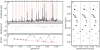 |
Fig. 11 Best-fit period-spacing pattern for TIC 374944608. Plots generated with the interactive code FLOSSY. (A): Lomb–Scargle periodogram (solid black line), observed periods (vertical dotted black lines), best-fit linear template (vertical red lines). Observed periods used for the fit are indicated with black triangles at the top. (B): deviations from the linear pattern (i.e., difference between the periods indicated by the black triangles and the red vertical lines). (C): period spacing as a function of mode period. Both black and white circles are the observations. The red markers are the best-fit linear pattern with slope α. Note that the fit is performed on p, not on ΔP, and missing mode periods in the observations create artificially larger ΔP values (white circles). (D): échelle diagram. The black circles are the periods used for the fit. The size of the circles is proportional to the amplitude of the amplitudes in the periodogram. The red markers are the best-fit linear pattern. The supplementary material contains a version of this figure for every pattern in our catalog. |
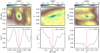 |
Fig. 12 Values of the cost function around the best-fit solution for TIC 374944608 shown in Fig. 11. Plots generated with the interactive code FLOSSY. Top: correlation plots. Bottom: minimum value of the cost function S as a function of the template period-spacing parameters. The supplementary material contains a version of this figure for every pattern in our catalog. |
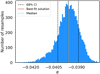 |
Fig. 13 Confidence interval (CI) for α following a bootstrap residual procedure for TIC 374944608. The meaning of the various vertical dashed lines are indicated in the legend. |
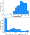 |
Fig. 14 Final catalog. Top: apparent TESS magnitude. Bottom: median contamination level in the aperture mask caused by flux of neighboring stars. |
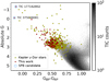 |
Fig. 15 Gaia color-magnitude diagram showing our sample (red) and the 611 γ-Dor stars with period-spacing patterns found by Li et al. (2020) in Kepler data (yellow). Stars marked with blue circles are SPB candidates. Background stars correspond to the TESS southern CVZ. Magnitudes are not corrected for extinction. |
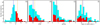 |
Fig. 16 Characterization of the best-fit patterns in our sample. The stacked histograms show retrograde modes in red and prograde modes in cyan. The vertical orange and blue lines are the median of the retrograde and prograde distributions, respectively. (A): slope α = dΔP/dP. (B): mean period 〈p〉. (C): mean period spacing 〈Δp〉. (D): span of the overtones. |
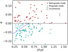 |
Fig. 17 p-α relation for g-mode pulsators in our catalog. The dashed blue line is the empirical cut from Fig. 8 in Li et al. (2020) that separates prograde ℓ = 1 g modes (bottom) from ℓ = 2 (top). The median of the uncertainties has been plotted as a typical uncertainty for a. Uncertainties in 〈p〉 are smaller than the symbol size. |
7 Summary
In this work, we present a new data analysis pipeline to create light curves from TESS full frame images (FFI), with an emphasis on the search for g-mode frequencies in intermediate-to high-mass stars. We present guidelines for extracting light curves from unprocessed TESS images, including the selection of aperture and background masks, the identification of time stamps affected by systematics in sectors 1–13 of the TESS southern CVZ, and a modified PCA to detrend the light curves. A color-magnitude criterion was presented as a method to identify main-sequence A/F- and O/B-type star candidates. We also introduced FLOSSY, an open source utility for inspecting periodograms of g-mode pulsators to facilitate searches for period-spacing patterns.
Based on the light curves extracted with our pipeline, we composed the first catalog of g-mode period-spacing patterns detected in TESS space photometry of dwarfs having colors representative of spectral types F to O. Our catalog contains 140 g-mode period-spacing patterns observed in 106 γ Dor stars and 2 SPB stars. The patterns were manually reviewed and contain g-mode frequencies having amplitudes of S/N > 4. In a future work, we will use the detected patterns to derive the internal rotation frequency near the convective core of the stars, as well as the buoyancy travel time across the stars (known as Π0). These two key quantities constitute important observables that are useful for performing asteroseismic modeling of intermediate-mass stars (e.g., Szewczuk & Daszyńska-Daszkiewicz 2018; Mombarg et al. 2021; Pedersen et al. 2021). The nominal frequency resolution of modes in the detected patterns amounts to 0.003d−1, following the 352 d long TESS southern CVZ light curves. This frequency resolution can be improved by a factor of 3 when the extended TESS Cycle 3 data will be included in the analysis. This will also lower the noise level in the Fourier domain and offers the future potential to detect more modes per star, as well as more stars with g-mode patterns. Our catalog and global properties of the detected patterns in it are publicly available through CDS. The patterns themselves, are shown in the supplementary material. This catalog constitutes a base for future ensemble asteroseismic modeling of TESS g-mode pulsators following methodologies as in Mombarg et al. (2021) or Pedersen et al. (2021). In this way, we will be able to constrain the internal physics of more rotating dwarfs with a convective core using the new available TESS data, in addition to the asteroseismic modeling achieved so far for a legacy sample of g-mode pulsators from the Kepler mission (Gebruers et al. 2021). This will increase the number of dwarfs with such modeling and will lead to a better understanding of the transport processes and their relationship to the internal rotation profile of these stars.
Acknowledgements
The research leading to these results has received funding from the European Research Council (ERC) under the European Union’s Horizon 2020 research and innovation programme (grant agreement no. 670519: MAMSIE) and from the KU Leuven Research Council (grant C16/18/005: PARADISE). TVR gratefully acknowledges support from the Research Foundation Flanders under grant agreement no. 12ZB620N. This research has made use of the SIMBAD database, operated at CDS, Strasbourg, France. This work made use of the Third Data Release of the GALAH Survey (Buder et al. 2021). The GALAH Survey is based on data acquired through the Australian Astronomical Observatory, under programs: A/2013B/13 (The GALAH pilot survey); A/2014A/25, A/2015A/19, A2017A/18 (The GALAH survey phase 1); A2018A/18 (Open clusters with HERMES); A2019A/1 (Hierarchical star formation in Ori OB1); A2019A/15 (The GALAH survey phase 2); A/2015B/19, A/2016A/22, A/2016B/10, A/2017B/16, A/2018B/15 (The HERMES-TESS program); and A/2015A/3, A/2015B/1, A/2015B/19, A/2016A/22, A/2016B/12, A/2017A/14 (The HERMES K2-follow-up program). We acknowledge the traditional owners of the land on which the AAT stands, the Gamilaraay people, and pay our respects to elders past and present. This paper includes data that has been provided by AAO Data Central (datacentral.aao.gov.au). This work has made use of data from the European Space Agency (ESA) mission Gaia (https://www.cosmos.esa.int/gaia), processed by the Gaia Data Processing and Analysis Consortium (DPAC, https://www.cosmos.esa.int/web/gaia/dpac/consortium). Funding for the DPAC has been provided by national institutions, in particular the institutions participating in the Gaia Multilateral Agreement. In addition to the software cited in the main body of the paper we have also made use of Lightkurve, a Python package for Kepler and TESS data analysis (Lightkurve Collaboration 2018), Astropy,6 a community-developed core Python package for Astronomy (Astropy Collaboration 2013, 2018), Matplotlib (Hunter 2007), NumPy (Harris et al. 2020), SciPy (Virtanen et al. 2020), pandas (Wes McKinney 2010). Finally, we would like to thank the anonymous referee for useful comments and suggestions.
Appendix A Extended tables and figures
Table A.1 lists the removed time intervals before the detrending of the light curves described in Sect. 3.2. The best-fit values of the parameters defined in Sect. 5 that characterize the 140 period-spacing patterns in our catalog are publicly available through CDS. The supplementary material available online contains a version of Figs. 11 and 12 that show the periodogram and the best-fit period-spacing pattern for all stars in our catalog. Whenever periods are plotted with gray circles in those figures, those periods are ignored in the fit.
Figure A.1 shows a negative correlation with a Pearson correlation coefficient of −0.34 and a p-value of 0.04 between the mean pulsation period of our catalog stars and their surface velocity estimated from spectral line broadening as reported in GALAH DR3 (Buder et al. 2021). In other words, larger surface velocities are measured for stars with shorter 〈P〉. While the measurement of the surface velocity from spectral line broadening is complicated and can never be precise in the presence of time-dependent gravity-mode velocity broadening (Aerts et al. 2014), this result is consistent with the expected effect of faster rotation on the periods of the pulsation modes (Bouabid et al. 2013). There is significant scatter in the figure, as expected for a sample of stars seen at random inclination angles, given the small overlap of only 38 stars between our catalog and GALAH DR3. Moreover, the uncertainties reported by GALAH DR3 are underestimates given that the spectral line broadening changes considerably throughout the pulsation cycles as shown by Aerts et al. (2014), while that time dependence has been ignored in the reported velocity estimates based on snapshot spectra. This precludes us to connect in-depth conclusions based on this correlation in Fig. A.1. Figure A.2 shows the distributions of mass, surface gravity, and effective temperature for our catalog stars available in GALAH DR3. The ranges of these three parameters are in agreement with those of γ Dor stars (Van Reeth et al. 2015b; Li et al. 2020).
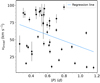 |
A.1 Correlation between the surface velocity deduced from spectral line broadening as reported by GALAH DR3 and our pattern parameter 〈P〉. If a star has multiple patterns, then the pattern with the highest-amplitude pulsations was used. The plot contains the 38 stars in common in GALAH DR3 and our catalog, where we only considered stars with spectra flagged as reliable in GALAH DR3. Uncertainties in 〈P〉 are smaller than the symbol size, while those of the velocities are underestimates for reasons explained in the text. |
Intervals excluded from the light curves.
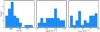 |
A.2 Histograms for the spectroscopic stellar parameters of the 38 stars in common with our catalog having spectra flagged as reliable in the GALAH DR3 catalog by Buder et al. (2021). |
References
- Aerts, C. 2021, Rev. Mod. Phys., 93, 015001 [Google Scholar]
- Aerts, C., Christensen-Dalsgaard, J., & Kurtz, D. W. 2010, Asteroseismology (Springer-Verlag: Heidelberg) [Google Scholar]
- Aerts, C., Simón-Díaz, S., Groot, P. J., & Degroote, P. 2014, A&A, 569, A118 [NASA ADS] [CrossRef] [EDP Sciences] [Google Scholar]
- Aerts, C., Van Reeth, T., & Tkachenko, A. 2017, ApJ, 847, L7 [Google Scholar]
- Aerts, C., Molenberghs, G., Michielsen, M., et al. 2018, ApJS, 237, 15 [Google Scholar]
- Aerts, C., Mathis, S., & Rogers, T. M. 2019, ARA&A, 57, 35 [Google Scholar]
- Antoci, V., Cunha, M. S., Bowman, D. M., et al. 2019, MNRAS, 490, 4040 [Google Scholar]
- Arenou, F., Luri, X., Babusiaux, C., et al. 2018, A&A, 616, A17 [NASA ADS] [CrossRef] [EDP Sciences] [Google Scholar]
- Astropy Collaboration (Robitaille, T.P., et al.) 2013, A&A, 558, A33 [NASA ADS] [CrossRef] [EDP Sciences] [Google Scholar]
- Astropy Collaboration (Price-Whelan, A.M., et al.) 2018, AJ, 156, 123 [NASA ADS] [CrossRef] [Google Scholar]
- Auvergne, M., Bodin, P., Boisnard, L., et al. 2009, A&A, 506, 411 [NASA ADS] [CrossRef] [EDP Sciences] [Google Scholar]
- Bailer-Jones, C. A. L., Rybizki, J., Fouesneau, M., Mantelet, G., & Andrae, R. 2018, AJ, 156, 58 [Google Scholar]
- Baran, A. S., & Koen, C. 2021, Acta Astron. 71, 113 [Google Scholar]
- Bouabid, M. P., Dupret, M. A., Salmon, S., et al. 2013, MNRAS, 429, 2500 [Google Scholar]
- Bowman, D. M. 2020, Front. Astron. Space Sci., 7, 70 [Google Scholar]
- Bowman, D. M., & Michielsen, M. 2021, A&A, 656, A158 [NASA ADS] [CrossRef] [EDP Sciences] [Google Scholar]
- Brasseur, C. E., Phillip, C., Fleming, S. W., Mullally, S. E., & White, R. L. 2019, Astrophysics Source Code Library [record ascl:1905.007] [Google Scholar]
- Buder, S., Sharma, S., Kos, J., et al. 2021, MNRAS, 506, 150 [NASA ADS] [CrossRef] [Google Scholar]
- Byrd, R. H., Lu, P., Nocedal, J., & Zhu, C. 1995, SIAM J. Sci. Comput., 16, 1190 [Google Scholar]
- Caldwell, D. A., Tenenbaum, P., Twicken, J. D., et al. 2020, Res. Notes Astron. Astrophys., 4, 201 [Google Scholar]
- Christophe, S., Ballot, J., Ouazzani, R. M., Antoci, V., & Salmon, S. J. A. J. 2018, A&A, 618, A47 [NASA ADS] [CrossRef] [EDP Sciences] [Google Scholar]
- Cunha, M. S., Avelino, P. P., Christensen-Dalsgaard, J., et al. 2019, MNRAS, 490, 909 [Google Scholar]
- Degroote, P., Briquet, M., Catala, C., et al. 2009, A&A, 506, 111 [NASA ADS] [CrossRef] [EDP Sciences] [Google Scholar]
- Degroote, P., Aerts, C., Baglin, A., et al. 2010, Nature, 464, 259 [Google Scholar]
- Eckart, C. 1960, Phys. Fluids, 3, 421 [Google Scholar]
- Feinstein, A. D., Montet, B. T., Foreman-Mackey, D., et al. 2019, PASP, 131, 094502 [Google Scholar]
- García, R. A., & Ballot, J. 2019, Liv. Rev. Sol. Phys., 16, 4 [Google Scholar]
- Gebruers, S., Straumit, I., Tkachenko, A., et al. 2021, A&A, 650, A151 [NASA ADS] [CrossRef] [EDP Sciences] [Google Scholar]
- Handberg, R., Lund, M., & Huber, D. 2019, https://doi.org/10.17909/t9-4smn-dx89 [Google Scholar]
- Handberg, R., Lund, M. N., White, T. R., et al. 2021, ApJ, 162, 170 [CrossRef] [Google Scholar]
- Harris, C. R., Millman, K. J., van der Walt, S.J., et al. 2020, Nature, 585, 357 [NASA ADS] [CrossRef] [Google Scholar]
- Hekker, S., & Christensen-Dalsgaard, J. 2017, A&ARv, 25, 1 [Google Scholar]
- Huang, C. X., Vanderburg, A., Pál, A., et al. 2020, Res. Notes Astron. Astrophys., 4, 204 [Google Scholar]
- Hunter, J. D. 2007, Comput. Sci. Eng., 9, 90 [NASA ADS] [CrossRef] [Google Scholar]
- Ijspeert, L.W., Tkachenko, A., Johnston, C., et al. 2021, A&A, 652, A120 [NASA ADS] [CrossRef] [EDP Sciences] [Google Scholar]
- Kaye, A. B., Handler, G., Krisciunas, K., Poretti, E., & Zerbi, F. M. 1999, PASP, 111, 840 [Google Scholar]
- Kippenhahn, R., Weigert, A., & Weiss, A. 2012, Stellar Structure and Evolution (Springer Berlin: Heidelberg) [Google Scholar]
- Koch, D. G., Borucki, W. J., Basri, G., et al. 2010, ApJ, 713, L79 [Google Scholar]
- Kurtz, D. W., Shibahashi, H., Murphy, S. J., Bedding, T. R., & Bowman, D. M. 2015, MNRAS, 450, 3015 [NASA ADS] [CrossRef] [Google Scholar]
- Lee, U. 2021, MNRAS, 505, 1495 [NASA ADS] [CrossRef] [Google Scholar]
- Li, G., Bedding, T. R., Murphy, S. J., et al. 2019, MNRAS, 482, 1757 [Google Scholar]
- Li, G., Van Reeth, T., Bedding, T. R., et al. 2020, MNRAS, 491, 3586 [Google Scholar]
- Lightkurve Collaboration, Cardoso, J.V.D.M., Hedges, C., et al. 2018, Astrophysics Source Code Library [ascl:1812.013] [Google Scholar]
- Loumos, G. L., & Deeming, T. J. 1978, Ap&SS, 56, 285 [NASA ADS] [CrossRef] [Google Scholar]
- Miglio, A., Montalbán, J., Noels, A., & Eggenberger, P. 2008, MNRAS, 386, 1487 [Google Scholar]
- Mombarg, J. S. G., Dotter, A., Van Reeth, T., et al. 2020, ApJ, 895, 51 [Google Scholar]
- Mombarg, J. S. G., Van Reeth, T., & Aerts, C. 2021, A&A, 650, A58 [NASA ADS] [CrossRef] [EDP Sciences] [Google Scholar]
- Montgomery, M. H., & O’Donoghue, D. 1999, Delta Scuti Star Newsletter, 13, 28 [NASA ADS] [Google Scholar]
- Ouazzani, R.-M., Salmon, S. J. A. J., Antoci, V., et al. 2017, MNRAS, 465, 2294 [Google Scholar]
- Ouazzani, R. M., Lignières, F., Dupret, M. A., et al. 2020, A&A, 640, A49 [NASA ADS] [CrossRef] [EDP Sciences] [Google Scholar]
- Pápics, P. I. 2012, Astron. Nachr., 333, 1053 [CrossRef] [Google Scholar]
- Pápics, P. I., Tkachenko, A., Van Reeth, T., et al. 2017, A&A, 598, A74 [Google Scholar]
- Pedersen, M. G., Chowdhury, S., Johnston, C., et al. 2019, ApJ, 872, Ll9 [Google Scholar]
- Pedersen, M. G., Aerts, C., Pápics, P. I., et al. 2021, Nat. Astron., 5, 715 [NASA ADS] [CrossRef] [Google Scholar]
- Prat, V., Mathis, S., Buysschaert, B., et al. 2019, A&A, 627, A64 [NASA ADS] [CrossRef] [EDP Sciences] [Google Scholar]
- Prat, V., Mathis, S., Neiner, C., et al. 2020, A&A, 636, A100 [NASA ADS] [CrossRef] [EDP Sciences] [Google Scholar]
- Ricker, G. R., Winn, J. N., Vanderspek, R., et al. 2015, J. Astron. Telescopes Instrum. Syst., 1, 014003 [Google Scholar]
- Ruppert, D. 2011, Statistics and Data Analysis for Financial Engineering (New York: Springer) [CrossRef] [Google Scholar]
- Saio, H., Takata, M., Lee, U., Li, G., & Van Reeth, T. 2021, MNRAS, 502, 5856 [Google Scholar]
- Schmid, V. S., & Aerts, C. 2016, A&A, 592, A116 [NASA ADS] [CrossRef] [EDP Sciences] [Google Scholar]
- Schwarzenberg-Czerny, A. 2003, in Interplay of Periodic, Cyclic and Stochastic Variability in Selected Areas of the H-R Diagram, ed. C. Sterken, ASP Conf. Series, 292, 383 [NASA ADS] [Google Scholar]
- Shibahashi, H. 1979, PASJ, 31, 87 [NASA ADS] [Google Scholar]
- Stassun, K. G., Oelkers, R. J., Paegert, M., et al. 2019, AJ, 158, 138 [Google Scholar]
- Szewczuk, W., & Daszynska-Daszkiewicz, J. 2018, MNRAS, 478, 2243 [NASA ADS] [CrossRef] [Google Scholar]
- Szewczuk, W., Walczak, P., & Daszynska-Daszkiewicz, J. 2021, MNRAS, 503, 5894 [NASA ADS] [CrossRef] [Google Scholar]
- Takata, M., Ouazzani, R. M., Saio, H., et al. 2020, A&A, 635, A106 [NASA ADS] [CrossRef] [EDP Sciences] [Google Scholar]
- Tassoul, M. 1980, ApJS, 43, 469 [Google Scholar]
- Tkachenko, A., Aerts, C., Yakushechkin, A., et al. 2013, A&A, 556, A52 [NASA ADS] [CrossRef] [EDP Sciences] [Google Scholar]
- Townsend, R. H. D., & Teitler, S. A. 2013, MNRAS, 435, 3406 [Google Scholar]
- Townsend, R. H. D., Goldstein, J., & Zweibel, E. G. 2018, MNRAS, 475, 879 [Google Scholar]
- Twicken, J. D., Caldwell, D. A., Jenkins, J. M., et al. 2020, TESS Science Data Products Description Document: EXP-TESS-ARC-ICD-0014 Rev F, Tech. Rep. 20205008729, NASA [Google Scholar]
- Van Beeck, J., Prat, V., Van Reeth, T., et al. 2020, A&A, 638, A149 [NASA ADS] [CrossRef] [EDP Sciences] [Google Scholar]
- Van Beeck, J., Bowman, D. M., Pedersen, M. G., et al. 2021, A&A, 655, A59 [NASA ADS] [CrossRef] [EDP Sciences] [Google Scholar]
- Van Reeth, T., Tkachenko, A., Aerts, C., et al. 2015a, A&A, 574, A17 [NASA ADS] [CrossRef] [EDP Sciences] [Google Scholar]
- Van Reeth, T., Tkachenko, A., Aerts, C., et al. 2015b, ApJS, 218, 27 [Google Scholar]
- Van Reeth, T., Tkachenko, A., & Aerts, C. 2016, A&A, 593, A120 [NASA ADS] [CrossRef] [EDP Sciences] [Google Scholar]
- Van Reeth, T., Mombarg, J. S. G., Mathis, S., et al. 2018, A&A, 618, A24 [NASA ADS] [EDP Sciences] [Google Scholar]
- Virtanen, P., Gommers, R., Oliphant, T. E., et al. 2020, Nat. Methods, 17, 261 [Google Scholar]
- Waelkens, C. 1991, A&A, 246, 453 [NASA ADS] [Google Scholar]
- Wes McKinney. 2010, in Proceedings of the 9th Python in Science Conference, eds. S. van der Walt, & J. Millman, 56 [CrossRef] [Google Scholar]
- Wu, T., & Li, Y. 2019, ApJ, 881, 86 [Google Scholar]
- Zong, W., Charpinet, S., Vauclair, G., Giammichele, N., & Van Grootel, V. 2016, A&A, 585, A22 [NASA ADS] [CrossRef] [EDP Sciences] [Google Scholar]
Descriptions about TESS quality flags can be found in the section “Data Product Overview” in https://outerspace.stsci.edu/display/TESS.
Flagged as attitude tweak, coarse pointing and desaturation event.
Flagged as safe mode.
Flagged as manual exclude.
All Tables
All Figures
|
Fig. 1 2MASS color-magnitude diagram showing the pairs of cuts in absolute magnitude and color defining candidate g-mode pulsators of spectral type O/B (cyan straight lines) and A/F (red straight lines) in K and J–K. The cyan and red circles are bona fide O/B- and A/F-type stars, respectively, while the retained dwarfs from the TIC in the southern CVZ are plotted in the background. The side histograms show the distribution of stars; the pairs of cuts enclose 95% of the respective bona fide stars. |
| In the text | |
|
Fig. 2 Square 20-by-20 pixels around TIC 38845463, TESS sector 1. The color bar is common to the three panels and shows a logarithmic scale of the flux in electrons per second. The red circle represents the target star while white circles indicate TIC neighboring stars down to four TESS magnitudes fainter with respect to the target star. The symbol sizes are inversely proportional to the TESS magnitude. Declination grids are 2′ apart. Left: median image of the target pixel file. Middle: panel with the final aperture mask (red shade) and background mask (gray shade) overplotted. The aperture mask results from the threshold parameter n = 20 (see text for explanation). Right: best fit based on the left panel used to estimate the level of contamination in the aperture mask due to flux from neighboring stars. The image was modeled as six 2D Gaussian functions plus a 2D plane. See Sect. 3.1 for further details. |
| In the text | |
|
Fig. 3 Our star sample without constraints on the aperture mask size (7385 sources, gray histogram) and after imposing a minimum size of 9 pixels (2162 sources, blue histogram). Other constraints described in Sect. 3.1 apply to both histograms. Left: sample distribution of the median aperture mask sizes, calculated per star over all TESS sectors. Middle: sample distribution of the TESS magnitudes. The dashed red line marks a magnitude value of 13.5. Right: median contamination level caused by neighboring stars, calculated per star over all TESS sectors. The dashed orange line marks a contamination of 5%. |
| In the text | |
|
Fig. 4 Blue histogram in the bottom shows the number of TESS sectors per star with a satisfactory aperture mask. The dark-gray histogram shows the mean contamination in each bin of the blue histogram. The dashed red line shows the cut for stars with at least 11 TESS sectors (a total of 1967 stars). |
| In the text | |
|
Fig. 5 Uncorrected light curves of TIC 30192406, showing in red the time intervals that have been excluded for all stars according to Table A.1. Sector 1 shows an example of jittering of the satellite. Sector 2 shows an example of scattered sunlight reflected by the Earth or the Moon. Sector 3 shows an example of systematic flux variability caused by the periodic re-pointing of the camera. |
| In the text | |
|
Fig. 6 First seven normalized principal components (PC; columns of the matrix U) from the background mask of TIC 374944608, sector 2. The PCs are displayed in ascending order with the first normalized PC at the bottom and manually set 0.25 units apart from each other for a better visualization. Only black normalized PCs have a level of scattering <10−4 (see Sect. 3.2) and were used for the detrending of the light curve. |
| In the text | |
|
Fig. 7 Final light curve for TIC 374944608 as derived from our developed pipeline discussed in Sect. 3. |
| In the text | |
|
Fig. 8 Number of potential g-mode pulsations with S/N ≥ 4 per star. Frequencies were deduced from Step 1 described in Sect. 4. Our sample of 1967 stars has 1108 stars that are not in compliance with our Step 1 criterion and those are not plotted. The dashed red line shows the cut used to select rich enough period-spacing pattern candidates, namely, stars with at least ten significant mode periods. This resulted in 369 candidate pulsators. |
| In the text | |
|
Fig. 9 Histogram following Eq. (9) for the frequencies of stars in our g-mode sample. The gray shade marks the background level that represents a random match among combination frequencies and the horizontal dashed gray line marks 3 times that level. The vertical red shows the intercept of the dashed gray line and the distribution; it marks ε = 0.0002 according to Eq. (9). Frequencies occurring to the left of this line have a 67% probability of corresponding to a genuine combination frequency. |
| In the text | |
|
Fig. 10 Number of frequencies remaining in our sample after each step in Sect. 4 is applied. The pie chart is based on the frequencies of the 369 stars after step 1 of our frequency analysis. The total number of frequencies is 10927. |
| In the text | |
|
Fig. 11 Best-fit period-spacing pattern for TIC 374944608. Plots generated with the interactive code FLOSSY. (A): Lomb–Scargle periodogram (solid black line), observed periods (vertical dotted black lines), best-fit linear template (vertical red lines). Observed periods used for the fit are indicated with black triangles at the top. (B): deviations from the linear pattern (i.e., difference between the periods indicated by the black triangles and the red vertical lines). (C): period spacing as a function of mode period. Both black and white circles are the observations. The red markers are the best-fit linear pattern with slope α. Note that the fit is performed on p, not on ΔP, and missing mode periods in the observations create artificially larger ΔP values (white circles). (D): échelle diagram. The black circles are the periods used for the fit. The size of the circles is proportional to the amplitude of the amplitudes in the periodogram. The red markers are the best-fit linear pattern. The supplementary material contains a version of this figure for every pattern in our catalog. |
| In the text | |
|
Fig. 12 Values of the cost function around the best-fit solution for TIC 374944608 shown in Fig. 11. Plots generated with the interactive code FLOSSY. Top: correlation plots. Bottom: minimum value of the cost function S as a function of the template period-spacing parameters. The supplementary material contains a version of this figure for every pattern in our catalog. |
| In the text | |
|
Fig. 13 Confidence interval (CI) for α following a bootstrap residual procedure for TIC 374944608. The meaning of the various vertical dashed lines are indicated in the legend. |
| In the text | |
|
Fig. 14 Final catalog. Top: apparent TESS magnitude. Bottom: median contamination level in the aperture mask caused by flux of neighboring stars. |
| In the text | |
|
Fig. 15 Gaia color-magnitude diagram showing our sample (red) and the 611 γ-Dor stars with period-spacing patterns found by Li et al. (2020) in Kepler data (yellow). Stars marked with blue circles are SPB candidates. Background stars correspond to the TESS southern CVZ. Magnitudes are not corrected for extinction. |
| In the text | |
|
Fig. 16 Characterization of the best-fit patterns in our sample. The stacked histograms show retrograde modes in red and prograde modes in cyan. The vertical orange and blue lines are the median of the retrograde and prograde distributions, respectively. (A): slope α = dΔP/dP. (B): mean period 〈p〉. (C): mean period spacing 〈Δp〉. (D): span of the overtones. |
| In the text | |
|
Fig. 17 p-α relation for g-mode pulsators in our catalog. The dashed blue line is the empirical cut from Fig. 8 in Li et al. (2020) that separates prograde ℓ = 1 g modes (bottom) from ℓ = 2 (top). The median of the uncertainties has been plotted as a typical uncertainty for a. Uncertainties in 〈p〉 are smaller than the symbol size. |
| In the text | |
|
A.1 Correlation between the surface velocity deduced from spectral line broadening as reported by GALAH DR3 and our pattern parameter 〈P〉. If a star has multiple patterns, then the pattern with the highest-amplitude pulsations was used. The plot contains the 38 stars in common in GALAH DR3 and our catalog, where we only considered stars with spectra flagged as reliable in GALAH DR3. Uncertainties in 〈P〉 are smaller than the symbol size, while those of the velocities are underestimates for reasons explained in the text. |
| In the text | |
|
A.2 Histograms for the spectroscopic stellar parameters of the 38 stars in common with our catalog having spectra flagged as reliable in the GALAH DR3 catalog by Buder et al. (2021). |
| In the text | |
Current usage metrics show cumulative count of Article Views (full-text article views including HTML views, PDF and ePub downloads, according to the available data) and Abstracts Views on Vision4Press platform.
Data correspond to usage on the plateform after 2015. The current usage metrics is available 48-96 hours after online publication and is updated daily on week days.
Initial download of the metrics may take a while.