| Issue |
A&A
Volume 661, May 2022
The Early Data Release of eROSITA and Mikhail Pavlinsky ART-XC on the SRG mission
|
|
|---|---|---|
| Article Number | A18 | |
| Number of page(s) | 15 | |
| Section | Numerical methods and codes | |
| DOI | https://doi.org/10.1051/0004-6361/202141099 | |
| Published online | 18 May 2022 | |
Systematic evaluation of variability detection methods for eROSITA
1
Max Planck Institute for Extraterrestrial Physics,
Giessenbachstrasse,
85741
Garching,
Germany
e-mail: This email address is being protected from spambots. You need JavaScript enabled to view it.
2
Dr. Karl Remeis-Observatory and Erlangen Centre for Astroparticle Physics, Friedrich-Alexander-Universität Erlangen-Nürnberg,
Sternwartstr. 7,
96049
Bamberg,
Germany
Received:
15
April
2021
Accepted:
3
December
2021
Abstract
The reliability of detecting source variability in sparsely and irregularly sampled X-ray light curves is investigated. This is motivated by the unprecedented survey capabilities of eROSITA on board the Spektrum-Roentgen-Gamma observatory, providing light curves for many thousand sources in its final-depth equatorial deep-field survey. Four methods for detecting variability are evaluated: excess variance, amplitude maximum deviations, Bayesian blocks, and a new Bayesian formulation of the excess variance. We judge the false-detection rate of variability based on simulated Poisson light curves of constant sources, and calibrate significance thresholds. Simulations in which flares are injected favour the amplitude maximum deviation as most sensitive at low false detections. Simulations with white and red stochastic source variability favour Bayesian methods. The results are applicable also for the million sources expected in the eROSITA all-sky survey.
Key words: methods: data analysis / stars: flare / X-rays: bursts / X-rays: galaxies / galaxies: active
© J. Buchner et al. 2022
 Open Access article, published by EDP Sciences, under the terms of the Creative Commons Attribution License (https://creativecommons.org/licenses/by/4.0), which permits unrestricted use, distribution, and reproduction in any medium, provided the original work is properly cited.
Open Access funding provided by Max Planck Society.
1 Introduction
The variability of astrophysical sources is a powerful diagnostic to differentiate between different physical models even when these models predict similar spectral energy distributions. Variability studies have enriched the zoo of astrophysical phenomena with new mysteries, including in recent years for example fast radio bursts (Lorimer et al. 2007; Petroff et al. 2019), ultra-luminous X-ray sources (e.g. Bachetti et al. 2014; Liu et al. 2013), and quasi-periodic eruptions (Miniutti et al. 2019). In high-energy astrophysics, the search for transient phenomena has a long history with gamma-ray bursts (Klebesadel et al. 1973; Gehrels & Mészáros 2012), for example. Missions such as MAXI (Matsuoka et al. 2009), RXTE (Swank 2006) and Swift (Gehrels et al. 2004) were explicitly designed to characterize the variable X-ray sky. However, these missions are sensitive only to the brightest objects (typically fewer than 100 variability triggers per year). This situation has changed with the launch of the eROSITA telescope on board SRG (Predehl et al. 2021), and its all-sky monitoring every six months in the first four years. Because eROSITA scans the X-ray sky rapidly over large areas down to faint fluxes, it has the potential to reveal a myriad of diverse variable and transient phenomena. Preliminary analysis of the first, most extreme events revealed gamma-ray burst afterglows (Weber 2020), super-soft emission from a classical nova (Ducci et al. 2020), flares in millisecond pulsars (Koenig et al. 2020), flares of unknown origin (Wilms et al. 2020), and new types of tidal disruption events (Malyali et al. 2021). These phenomena exhibit different variability behaviour (e.g. flares or red noise). To fully exploit the eROSITA data set, we require robust and well-characterised techniques to identify, classify, and characterise the variability properties of each detected X-ray source.
Identifying source variability in the X-rays is no small task. In the recent large-scale optical photometric surveys (Gaia, Zwicky Transient Factory, Optical Gravitational Lensing Experiment, etc.), systematics typically dominate measurement uncertainties, requiring a machine learning classifier to postprocess various classical light-curve summary statistics (Debosscher et al. 2007; Kim et al. 2011; Palaversa et al. 2013; Masci et al. 2014; Armstrong et al. 2016; Holl et al. 2018; Heinze et al. 2018; Jayasinghe et al. 2019; van Roestel et al. 2021). In contrast, for repeated X-ray surveys in which most X-ray sources are found near the detection limit, statistical (Poisson) uncertainties are dominant. In this regime, methods such as fractional variance (Edelson et al. 1990), excess variance (Nandra et al. 1997), and Bayesian blocks (Scargle et al. 2013) have been proposed. However, their application has typically been limited to a handful of light curves at a time. De Luca et al. (2021) investigated variable objects of the archival XMM-Newton X-ray sky with Bayesian blocks and light-curve summary statistics. eROSITA detected almost a million point sources already in its first all-sky survey (eRASS1), and a new all-sky survey with similar characteristics is conducted every six months. With this large number of sources, the calibration of the instrument and detection methods becomes important to avoid both false positives and false negatives in large numbers. Additionally, the eROSITA scanning pattern imprints strong temporal modulations of the effective instrument sensitivity at any particular sky location. To summarise, any useful method must consistently distinguish Poisson and sensitivity fluctuations from variations intrinsic to the astrophysical source. For these reasons, we have examined the performance of commonly used variability analysis methods, together with a novel Bayesian approach, within the eROSITA regime.
This paper investigates the reliability and sensitivity of various variability detection methods, based on a pilot eROSITA survey over a extragalactic field of 140 square degrees. Its characteristics, such as exposure depth, are similar to the final stacked eight-year all-sky surveys. Classes of variable sources expected include flaring X-ray stars and variable active galactic nuclei. The properties of that data set is presented in Sect. 2, including how counts are extracted in time bins. Various ways for constructing light curves (Sect. 3.1) and visualising them (Sect. 3.2) are discussed. These light curves form the foundation for the considered variability detection methods, which are presented in detail in Sect. 3.3. Section 3.4 explains our method for evaluating and comparing the methods, based on extensive numerical simulations (Sect. 3.5). The results section presents the calibrations needed for a reliable use of the methods (Sect. 4.1) and how sensitive they are to various types of variability (Sect. 4.2). We conclude with discussing in Sect. 5 the advantages of a method that we newly developed in this work, Bayesian excess variance, and its future use for eROSITA and beyond.
2 Data
The eROSITA Final Equatorial-Depth Survey (eFEDS) field was observed with eROSITA in November 2019. The source catalogue paper (Brunner et al. 2022) presents the observations, eROSITA analysis software, and data treatment. Survey aspects that are important for investigating source variability are highlighted in this section. The depth expected after completion of all eROSITA all-sky survey scans was reached and slightly exceeded in the eFEDS field. eFEDS consists of four adjacent, approximately rectangular areas aligned with the ecliptic coordinate grid, which were covered from ecliptic east to west by a sequence of linear scans going from ecliptic north to south and back. The typical scanning speed was 13.15 ”/s (Brunner et al. 2022). Because the field of view of eROSITA is about ten times larger than the distance between scans, each source was covered multiple times. The resulting cadence is such that sources were visible continuously for several minutes, and were revisited approximately every hour. The black curve of Fig. 1 illustrates this strongly variable instrument sensitivity over time for a typical source. This illustrates the difference between eROSITA survey light curves and those of typical pointed observations, where the instrument sensitivity is nearly constant. Therefore different analysis methods are required. In eFEDS, 27910 point sources were detected (Brunner et al. 2022) in the 0.2–2.3 keV band. These form the main eFEDS sample, which is also the basis of this paper.
For all 27910 sources, a spectrum and light curve was extracted. The procedure is described in detail in Liu et al. (2022). Source counts were extracted from a circular aperture with a radius of ≈20–40” (increasing with source counts). A representative local background was extracted from an annular region, also centred at the source position. The inner and outer radii of the annulus were scaled to be 5 and 25 times larger than the source radius, which yielded a ratio of background to source area of r' ≈ 200. Because most eROSITA observations are made in scanning mode, these extraction regions are defined in terms of sky coordinates (rather than on some instrumental coordinate system). Neighbouring sources were masked from the source and background regions before extraction, and finally, the light curves from the seven telescope modules were summed (see Liu et al. 2022). Figure 1 shows an example of counts extracted over time for a bright source, with the background counts scaled according to the area ratio. The count statistics are low and therefore in the Poisson regime.
Light curves were extracted in three bands. Their energy ranges are 0.2–5 (full band, band 0), 0.2–2.3 (soft band, band 1), and 2.3–5 keV (hard band, band 2). Here, we focus primarily on the soft, and secondarily on the properties of the hard-band light curves. Because the X-ray response of eROSITA is relatively soft, the full band is dominated by and nearly identical to the soft band for most detected sources.
Light curves with time bins of 100s were constructed using srctool1 (Brunner et al. 2022, version eSASSusers_201009). This binning choice balances samples times during the survey track as well as revisits. The effective sensitivity of eROSITA to an astrophysical source varies with time, as the source moves through the field of view of the telescope modules and becomes zero in time bins while the source is outside the field of view. The dimensionless fractional exposure (fexpo) parameter (range 0–1) computed by srctool is an estimate of the effective sensitivity of the instrument within a time bin to the source in question. The computation of fexpo for each bin of the light curve was carried out by integrating the instantaneous effective response of the instrument within the bin on a time grid comparable to the instrumental integration time (Delta t = 50 ms). The computation of fexpo takes into account the geometry of the source extraction aperture, the telescope attitude, off-axis vignetting, energy- and position-dependent point spread function (PSF), good time intervals, instrument dead time, and the location of any bad pixels, and it was carried out independently for each of the seven telescope modules. An effective spectral index of Gamma = 1.7 is assumed when weighting the energy-dependent components of the instrument response model (vignetting, PSF) across broad energy bins. We normalised fexpo relative to the response expected for an on-axis point source observed with all telescope modules, assuming no extraction aperture losses. The black curve of Fig. 1 gives an example of the fexpo windowing for an arbitrarily chosen source in eFEDS, decreasing when the source is at the border of the field of view. Figure 2 shows the fexpo of all time bins for sources in the eFEDS field. Because the current understanding of the eROSITA vignetting function is somewhat uncertain at large off-axis angles, we only considered time bins exposed to fexpo > 0.1. This cut tends to segment the light curves into disjoint intervals that are filled with meaningful data. As the reflectivity of the eROSITA optics reduces at higher energies and large grazing angles, the hard band has a smaller effective field of view and systematically lower fexpo values (see Fig. 2). Unless otherwise stated, the remainder of this paper assumes that fexpo represents the relative sensitivity of the instrument correctly.
The cadences effectively sampled by the light curves are summarised in Fig. 3. The top panel illustrates that sources are typically observed over a span of four to seven hours. During this time, the light curves exhibit several gaps (see Fig. 1), during which other parts of the field were scanned. Typically, there are 4 to 12 blocks of contiguous observations (middle panel of Fig. 3), lasting not more than a few minutes each. This results in two effective cadences: consecutive exposures lasting a few minutes, and re-visits on timescales of hours.
For each time bin, the observed source counts S and background counts B are listed. Figure 4 presents histograms of these counts for the soft (blue) and hard (orange) band. For most time bins, the number of counts is in the single digits, contributed by sources near the detection threshold. eROSITA is most sensitive in the soft band, which typically shows more counts (up to 100 cts/bin), approximately 20 times higher than the maximum seen in the hard band. The expected number of background counts in each time bin is typically below 1. Light curves are presented in Boller et al. (2022), and significantly variable sources are identified. The focus of this work is to investigate methods for determining whether sources are significantly variable.
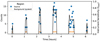 |
Fig. 1 Example counts of the tenth brightest eFEDS source. The markers indicate the number of counts from a single eROSITA telescope module in 100s time bins, recorded over a six-hour period. The black curve shows the sensitivity to the source position over time. |
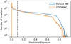 |
Fig. 2 Distribution of fractional exposure (fexpo) values for all light-curve time bins. |
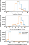 |
Fig. 3 Light-curve cadence summary statistics. Top panel: the time between first and last exposed time bins for each light curve, with typical values of four to seven hours. As Fig. 1 illustrates, the light curves are segmented into blocks. Middle panel: number of blocks, which ranges from 4 to 12. Bottom panel: duration of the longest block for each light curve, which typically lasts only a few minutes. |
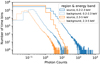 |
Fig. 4 Source and background photon-count distribution in the soft and hard bands. The background counts are scaled by the ratio of source to background area. |
3 Methods
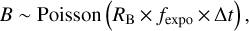
The counts observed in a time bin t can be expressed as a Poisson process, which integrates the band count rate R, dampened by the efficiency fexpo within the time interval ∆t. For the background region and assuming fexpo is constant within the time bin, this can be written as
 (1)
(1)
where C ~ Poisson(λ) means “counts C is a Poisson random variable with a mean of λ ”The total counts in the source region, S, contain contributions from the source, with count rate RS and background,
 (2)
(2)
The background rate RB is scaled by the area ratio of source and background extraction regions, r, with values near 1% being typical. The unknowns are RB, the background count rate, and RS, the net (without background) source count rate. Typical values for RS/(RB × r) are 8 for the soft band and 1 for the hard band.
3.1 Methods for inferring the source count rate per bin
In the following, we present two approaches for inferring the net count rate RS in each time bin. The first uses Gaussian approximations, while the second fully considers the Poisson nature of the data.
3.1.1 Classic per-bin source rate estimates
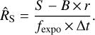
The classic point estimator for the net source count rate RS is
 (3)
(3)
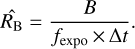
Here, the background count rate in the background region is estimated with
 (4)
(4)
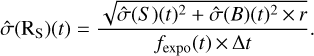
The uncertainty in the net source count rate  is estimated as
 (5)
(5)
Here,  (with C either S or B) is the uncertainty of the expected number of counts, given the observed counts C. One possibility is to use the simple
  estimator. However, in the low-count regime, the uncertainties are then severely underestimated (e.g. when S = 0). This leads to a strong count-dependent behaviour of any method that ingests these uncertainties.
Confidence intervals for the Poisson processes have been studied extensively in the X-ray and gamma-ray astronomy literature (e.g. Gehrels 1986; Kraft et al. 1991). They are asymmetric in general for realistic settings, and thus cannot be readily propagated in Eq. (5). We adopted the upper confidence interval formula  from Gehrels (1986) and also used it as a lower confidence interval instead of the formula
  This conservative choice tends to enlarge the error bars, and thus makes the data appear less powerful than they actually are. An alternative that is being considered for future releases of srctool are maximum likelihood-derived confidence intervals found by numerically exploring profile likelihoods (Barlow 2003).
3.1.2 Bayesian per-bin source rate estimates
A drawback of the estimates above is the Gaussianity error propagation. In the low-count regime, the Poisson uncertainties become asymmetric. We adopted the approach of Knoetig (2014) to propagate the uncertainties in a Bayesian framework.
Firstly, the unknown background count rate RB(t) only depends on known quantities in Eq. (1). The Poisson process likelihood, Poisson(C|λ) = λk × e−λ/k!, can be combined with a flat, improper prior on the expected count rate λ = RB ×fexpo, to define a posterior that can be numerically inverted using the inverse incomplete Gamma function Γ−1 (see also Cameron 2011). Specifically, the q-th quantile of the posterior probability distribution of RB (t) can be derived as Γ−1 (B + 1, q) × r/fexpo. The same approach cannot be applied to RS because it depends on the values of Sand RB(t) (Eq. (2)). We thus computed the marginalised likelihood function of the source rate RS as
 (6)
(6)
 (7)
(7)
In practice, Eq. (6) is evaluated by numerically integrating over q in a grid (see Knoetig 2014, for an alternative method).
The goal is then to place constraints on RS using the likelihood function P(S|Rs). Evaluating a grid over RS(t) over a reasonable range (logarithmically between 0.01 and 100 cts/s) explores the likelihood function of Eq. (6). If the grid points are interpreted to be equally probable a priori, quantiles (median, 1σ equivalents) can then be read off the normalised cumulative of P(S |Rs) grid values, and form Bayesian alternatives for  and
and  . A different approach to the priors on RS is explored below in Sect. 3.3.4.
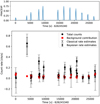 |
Fig. 5 Visualisations. Top panel: fractional exposure over time for an example source with 10 passes. Bottom panel: light curve of a simulated source with constant count rate and a bright flare. Black circles show the total counts without background subtraction, and red points show the expected background count rates in the source region (Eq. (4)). Grey error bars show classical net source count-rate estimates (Eqs. (3) and (5)). Black error bars show Bayesian net source count-rate posterior distributions, represented visually with 10, 50, and 90% quantiles under a log-uniform prior (Eq. (7)). |
3.2 Visualisations
The per-bin estimates defined above provide the possibility of plotting time series of inferred source count rates (a light curve). An example (simulated) light curve is shown in Fig. 5 with both classical and Bayesian error bar estimates. The classical confidence intervals are symmetric and sometimes include negative count rates. The Bayesian estimates are asymmetric and always positive.
Some forms of variability can then be judged by identifying whether the count rates are consistent over time. In Fig. 5, a major flare near t = 4000 s and perhaps two minor flares may be identified. One shortcoming of this approach is that the judgment by eye is subjective and difficult to reproduce. The Poisson fluctuations are also not intuitive (only one real flare was injected in this simulated time series). Nevertheless, insight can be gained by trying to understand which various methods “see”, and trying to understand what likely triggered a statistical test. They are also useful for judging the plausibility of the data under current calibration. For example, if the fractional exposure fexpo is misestimated at large off-axis angles, the count rates are enhanced or reduced while the source enters and leaves the field of view. These systematic over- or undercorrections can become visible as U or inverse-U-shaped light curves.
The binning of the time series also influences the visualisation. Large time bins may average out short-term variability. Small time bins may contain too few counts and thus large uncertainties. The accumulation of nearby data points is difficult to do by eye. However, this can be important, as variations are typically correlated on short timescales.
Cumulative counts address some of these limitations. Figure 6 plots the cumulative counts in the source region, S, over time as a red curve. In the last time bin, all counts are noted. To judge whether this light curve was variable, we generated Pois-son counts for 1000 simulated time series assuming a constant source, following Eq. (2). To do this, we assumed the classically inferred source and background count rates. The generated counts are shown in Fig. 6, with the mean as a dashed black curve and intervals corresponding to 1, 2, and 3σ as grey shadings. Near 4000 s, the red curve for this source departs above the 3σ range, indicating an excess of counts at that time (consistent with Eq. (5)). At the other times, the variations are within the 3σ intervals.
The benefit of the cumulative count plot is that it is independent of any binning. It stacks the information of neighbouring time bins. Instead of modifying the data through background subtraction, the data are fixed. A drawback is that time intervals cannot be investigated in isolation, as all time bins are correlated to the time bins before. Furthermore, these visualisations are not rigorous statistical variability tests, as the data will lie outside the 3σ regions occasionally, given enough time bins.
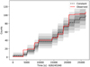 |
Fig. 6 Cumulative count visualisation. The red curve shows the observed cumulative counts over time. The expectation of a constant source is indicated as a dashed curve and grey intervals corresponding to 1, 2, and 3σ. |
3.3 Methods for variability detection
In this section, methods for detecting and quantifying variability are compared. In eFEDS, the time series are sparsely sampled (see Sect. 2). Within a total length of only a few hours, each source is typically continuously observed for a few minutes, about N ~ 20 times (less often at the edges of the field). In this setting, we tested several methods for their ability to detect variability, and quantified how sensitive they are to different types of variability.
3.3.1 Amplitude maximum deviation methods
The simplest definition of variability is that two measured source rates disagree with each other. This implies that the source has changed.
Assuming Gaussian error propagation, Boller et al. (2016) defined the amplitude maximum deviation (ampl_max) as the difference between the most extreme points,
 (8)
(8)
where tmin and tmax are the time bins with the lowest and highest  source rate estimate. The ampl_max is the distance between the lower error bar of the maximum value to the upper error bar of the minimum value. By comparing the span to the error bars, the significance can be quantified in units of standard deviations (i.e. as a z-score),
 (9)
(9)
This method is conservative, as it considers the error bars twice. A drawback of this method is the assumption that the errors are Gaussian. With the asymmetric Poisson errors derived in Sect. 3.1.2, we might define an analogous Bayesian AMPL_MAX and AMPL_SIG by modifying Eq. (9) to use the Bayesian quantile uncertainties instead of  . Such a modified method was considered for the simulations performed in this paper. However, it yielded a comparable efficiency in detecting variability. This is probably because this method is limited primarily by considering only the two extreme data points, rather than by a refinement of the error bars.
The amplitude maximum deviation quantifies both the size of the effect (Eq. (8)) and its statistical significance (Eq. (9)). Because only the two most extreme data points are considered, it is thus insensitive to the variations in the other values.
3.3.2 Bayesian blocks
The Bayesian blocks algorithm of Scargle et al. (2013) identifies in a sequence of measurement points where the rate changed. This adaptive binning technique automatically segments a light curve into blocks of constant rates separated by change points. The criterion for deciding the number and location of the change points is based on Bayesian model comparison. For a certain class of likelihood functions, Scargle et al. (2013) derived analytic recursive formulas that quickly construct the globally optimal segmentation. Bayesian blocks can be applied to photon counts of binned light curves and even to individual photon-count arrival times, thus not requiring a predefined binning. However, as Fig. 1 illustrates, the eROSITA photon counts are highly variable as the source runs through the field of view in the survey scan, simply because of angle-dependent instrument sensitivity. For astrophysical inference, we are interested in source variability, rather than observation-induced variability. The Bayesian blocks algorithm could be extended with a new likelihood to incorporate this information. However, a further difficulty is that the background is not negligible for most sources. Some of its components are variable over time, especially those passing through the mirrors and those sensitive to spacecraft orientation relative to the Sun. Others, such as the particle background, are persistent, and become dominant at large off-axis angles. An extension of Bayesian blocks to analyse source and background region light curve simultaneously would be desirable, building on the foundations outlined above. However, this is beyond the scope of this work. Therefore, we resort to the classic source rate and uncertainty estimators  and
and  , which are corrected for the fractional exposure, and use the Gaussian Bayesian blocks implementation from astropy (Astropy Collaboration 2013, 2018). This requires prebinned light curves, however.
In our application to binned light curves, all borders between time bins with observations are candidates for change points. Bayesian blocks begins with the hypothesis that the count rate is constant. For each candidate change point, it tries the hypothesis that the count rate is constant to some value before the change point, and constant to some value after the change point. The two hypothesis probabilities are compared using Bayesian model comparison. If the model comparison favours the split, each segment is analysed with the same procedure recursively. Finally, Bayesian blocks returns a segmented light curve and estimates for the count rate in each segment with its uncertainties.
The Bayesian model comparison requires a prior on the expected number of change points ncp. We adopted the prior favoured by simulations of Scargle et al. (2013),  with the desired false-positive rate set to po = 0.003 (corresponding to 3σ). Variability is significantly detected by the Bayesian blocks algorithm when it identified at least one change point. We refer to ncp as NBBLOCKS.
3.3.3 Fractional and excess variance
A Poisson process is expected to induce stochasticity into the measurement. Excess variance methods (Edelson et al. 1990, 2002; Nandra et al. 1997; Vaughan et al. 2003; Ponti et al. 2014) quantify whether the observed stochasticity shows additional variance, that is, is overdispersed.
Across bins, the mean net source count rate ṜS is
 (10)
(10)
The observed variance of the net source count rates  (one in each time bin) is
 (11)
(11)
The Poisson noise expectation is computed with the mean square error computed from the error bars,
 (12)
(12)
Subtracting off this expectation, we obtain the excess variance,
 (13)
(13)
Normalising to the mean count rate gives the normalised excess variance (NEV),
 (14)
(14)
The variable fraction of the signal, Fvar, also known as the fractional root-mean-square (RMS) amplitude, is then defined as
 (15)
(15)
The excess variance  quantifies the overdispersion, without making assumptions about the process causing the variability. Values of
  can also become negative by chance, however, or when the measurement uncertainties are overestimated. To avoid this problem (which affects Fvar), we forced NEV to not go below a low positive value (0.001).
Quantifying the significance of the excess variance is more difficult (Nandra et al. 1997). Vaughan et al. (2003) used simulations to determine the empirical formulas (valid for N from 2 to 2000 and Fvar from 0 to 40%) for the uncertainty in the NEV and Fvar estimators,
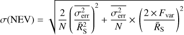 (16)
(16)
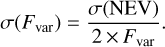 (17)
(17)
The significance of the excess variance can then be defined as FVAR_SIG = Fvar/σFvar) and NEV_SIG = NEV/σ(NEV).
3.3.4 Bayesian excess variance (bexvar)
The excess variance computation above assumes symmetric, Gaussian error bars. This limitation can be relaxed by modelling the entire data-generating process. Towards this, we assumed that at any time bin i, the rate RS(ti) is distributed according to a log-normal distribution with unknown parameters,
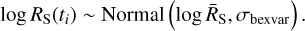 (18)
(18)
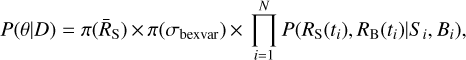
In this formulation, we need to estimate the mean logarithmic net source count rate (logṜS), the intrinsic scatter σbexvar, and the rates at each time bin RS(ti), giving N + 2 parameters. Equation (18) defines a prior for the source count rate of each bin. This is a hierarchical Bayesian model (HBM), combined with Eqs. (1) and (2), which define the probabilities in each time bin. Figure 7 illustrates the relation between all quantities as a graphical model.
Priors for ṜS and σbexvar also need to be chosen. Here, we simply used uninformative, wide flat priors,
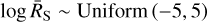 (19)
(19)
 (20)
(20)
The mean count rate ṜS has a straightforward interpretation. In its posterior distribution, the Poisson uncertainty is directly incorporated.
Variability is quantified with σbexvar, which gives the intrinsic variance. This log-scatter on the log-count rate is a different quantity than the excess variance on the (linear) count rate, σXS. Because the variability is defined as a log-normal, this corresponds to the log-amplitude of a multiplicative process. The motivation for this is primarily practical. Variable objects can be identified when the posterior distribution of σbexvar excludes low values. Here, we defined SCATT_LO as the lower 10% quantile of the posterior, and used it as a variability indicator.
The question now is how these formulas can be solved to produce probability distributions on σbexvar, for instance. The first step is the posterior probability computation. If we assume a source count rate RS(ti) at each bin, Eq. (2) indicates how the Poisson probability is to be computed to detect the source region counts S. The background count rate RB(ti) also needs to be chosen, and the Poisson probability to detect the background region counts B can be computed. If we further assume a value ṜS and σbexvar, Eq. (18) computes the probability of the N chosen RS(t) values. Finally, Eqs. (19) and (20) specify the prior probability for ṜS and σbexvar, that is, π(ṜS) and π(σbexvar), respectively. To summarise, given the assumed (2 × N + 2)-dimensional parameter vector, we computed 2N + 3 probabilities for light-curve data D = (S1, B1, … SN, BN),

As we required all probabilities to hold simultaneously, we multiplied them, obtaining the posterior probability function,
 (21)
(21)
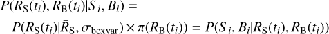
where the per-bin posterior probability terms
 (22)
(22)
and the per-bin likelihoods are the product of Eqs. (1) and (2),
 (23)
(23)
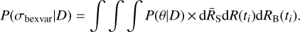
This provided a posterior over a (2 × N + 2)-dimensional parameter space. To compute probability distributions for a parameter of interest, for example, σbexvar, all other parameters need to be marginalised out,
 (24)
(24)
The exploration of the posterior probability distribution on σbexvar can be achieved with Markov chain Monte Carlo algorithms. These repeatedly propose values θ and sample the values of σbexvar proportional to their posterior probability. However, in practice, the convergence of this computation is slow and not always stable, even with recent advanced methods.
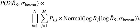
Substantial improvements are possible for rapid computation. Firstly, Sect. 3.1.2 already derived the marginalised likelihood for the per-bin source rates P(S,B|RS). These can be represented as an array Pi,j giving the probability for time bin i over a grid of source rates Rj. Using the normal distribution defined by ṜS and σbexvar), we can compute at each grid R(t) value its probability, and marginalise over j over the grid for each time bin. Thus, we approximate Eq. (21) with
 (25)
(25)
This leaves only a two-dimensional probability distribution. We employed the nested sampling Monte Carlo algorithm MLFriends (Buchner 2016, 2019) implemented in the UltraNest Python package2 (Buchner 2021) to obtain the probability distribution P(σbexvar|D) uing the likelihood (Eq. (25)) and priors (Eqs. (19) and 20).
The probability distribution P(σbexvar |D) quantifies the variability amplitude supported by the data. To illustrate the typical behaviour of this probability distribution, the highest values of σbexvar are excluded and receive a low probability after a few data points are added. When inconsistent data points (excess variance) is present, the lowest values of σbexvar also receive a low probability, concentrating the probability distribution near the true value. Therefore, a conservative indicator of the magnitude of the excess variance is the lower 10% quantile of the distribution, which we call SCATT_LO. We adopted this single summary statistic for comparison with the other methods. Similar to the other methods (NEV and Bayesian blocks), the significance quantification needs to be obtained with simulations.
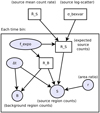 |
Fig. 7 Graphical model of the Bayesian excess variance method. Shaded circles indicate known values, related to the experiment setup or observed data. Rectangles indicate unknown parameters, including the unknown source count rate and the count rate in each time bin. An arrow from A to B indicates that the generation of B was influenced by A. |
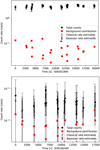 |
Fig. 8 Simulated light curves of constant sources with Poisson noise. Black circles show the total counts without background subtraction, and red points show the expected background count rates in the source region (Eq. (4)). Top panel: source with a high count rate with a constant 3 cts/s, where the source counts are always above the expected background counts. Bottom panel: source with a low count rate with a constant 0.03 cts/s, where source region counts and background counts are comparable and show substantial Poisson scatter. Grey error bars show classical net source count-rate estimates (Eqs. (3) and 5). Black error bars show Bayesian net source count-rate posterior distributions (Eq. (7)). |
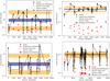 |
Fig. 9 As in Fig. 8, but for gaussvar sources. The intrinsic count rate is randomly varied following a log-normal distribution around a baseline count rate. Left panels: cases with σ = 1dex variations, clearly visible in the scatter of the total counts (black points) in both bright (top panel) and faint (bottom panel) sources. Right panels: lower variations (σ = 0.1 dex). In the bright case (top panel), the scatter of the black points is substantially larger than the error bars, while in the faint case (bottom), the error bars overlap. In the top panel the background contribution (red points) is well below the total counts (black), while in the bottom panel, they are comparable. The solid blue line and band show the posterior median and 1a uncertainty of the intrinsic source count rate |

3.4 Method comparison
To summarise, we considered four methods: amplitude Maximum Deviation, Normalised Excess Variance, Bayesian Blocks and Bayesian Excess Variance. Their estimators are AMPL_SIG, NEV_SIG, NBBLOCKS and SCATT_LO. All of these methods rely on binned light curves. They are therefore sensitive to the chosen number of bins, which modulates how much information is contained in each bin. All methods neglect time information and are oblivious to the order of measurements. The exception is Bayesian blocks. All methods disregard gaps.
To quantify the significance of a detection, the first three methods already have a significance indicator (AMPL_SIG, NEV_SIG, and NBBLOCKS). However, these are derived under specific assumptions or simulation settings: The existing simulations of Vaughan et al. (2003) and Scargle et al. (2013) did not consider the scenario with variable sensitivity and non-negligible backgrounds. The AMPL_SIG does not account for the number of data points, which increase the chance of obtaining a large AMPL_MAX by chance. The Bayesian blocks, NEV, and AMPL_SIG methods adopt imperfect Gaussian approximations. Because of these limitations, simulations are necessary to detect variable objects with the desired reliability characteristics. For these reasons, we verified that the significance indicators correspond to the desired p-values, for example, in constant sources NEV_SIG should exceed 3σ only in 0.1% of cases by chance. We preferred to verify NEV_SIG and AMPL_SIG rather than NEV and AMPL_MAX, as the existing formulae already largely correct for trends with size of the uncertainties and the number of data points. In Bayesian blocks, unjustified change points should also rarely be introduced by chance.
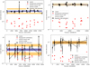 |
Fig. 10 As in Fig. 9, but for flare sources. The count rate in one bin is increased by a factor of k. The top (bottom) panels: bright (faint) source baseline count rates. Top panels: flare of k = 10, and bottom panels: k = 2 flare. |
3.5 Simulation setup
To calibrate the significance threshold at which an object is classified as variable, we used extensive simulations. Four data sets were generated. Each data set was created based on the 27 910 eFEDS light curves, taking their time sampling (∆T) and fexpo values as is. This generated a data set under identical conditions. We did not vary the vignetting and other corrections, that is, we assumed that the instrument model was correct. Background counts were sampled using Eq. (1) with Poisson random numbers assuming the measured time-average  as a constant across all time bins for that source. Source counts were sampled using Eq. (2) with Poisson random numbers, using the sum of the scaled background rate and the desired source rate R(t) at that time step. For reasonable ranges of R(t), we recall that the typical number of counts in a 100 s bin is below 10 for most sources and time bins, but can reach up to a few hundred (see Fig. 4 and Boller et al. 2022). We therefore considered count-rate ranges between μ = 0.03 cts/s and 3 cts/s.
For the source rate, four scenarios were considered as described below.
constant: the count rate is constant: R(t) = μ. The sample is divided into five equally sized groups. Each group is assigned a different count rate (0.03, 0.1, 0.3, 1, and 3 cts/s). Figure 8 presents two examples of constant light curves, showing the lowest and highest count rates considered. The Poisson scatter is strongly noticeable.
gaussvar: for each time bin, a count rate is drawn independently from a log-normal distribution with mean log μ and variance σ: log R(t) ~ Normal(log μ, σ). The sample is divided into five equally sized groups. Each group is assigned a different mean count rate (μ =0.03, 0.1, 0.3, 1, and 3 cts/s). The groups are further subdivided into five subgroups. Each subgroup is assigned a different variance (σ = 0.03,0.1, 0.3, 0.5, and 1.0). This represents the behaviour of long-term revisits of AGN (e.g., Maughan & Reiprich 2019). Figure 9 presents four examples of gaussvar light curves, varying the intrinsic count rates (left vs. right panels) and the strength of the intrinsic scatter (top vs. bottom panels). These examples also illustrate the inference of bexvar, estimating the mean intrinsic count rate (blue line), its uncertainty (blue band), the count-rate log variation (orange lines), and its uncertainty (orange bands).
flare: same as constant, but in one randomly selected time bin, the count rate is increased by a factor k. The groups are subdivided into subgroups. Each subgroup is assigned a different factor (k = 30,10, 5, 2, 1.5, and 1.3). The subgroups with k =30 and 5 are half as large as the other subgroups. Figure 10 presents four examples of flare light curves, varying the intrinsic count rates (left vs. right panels) and the flare strength k (top vs. bottom panels). Weak flares become difficult to notice in the presence of Poisson noise.
redvar: to complement the white-noise process in gaussvar, a correlated random walk (red noise) is also tested. Specifically, we adopt a first-order Ornstein-Uhlenbeck process
 . This generates on short timescales a power-law power spectrum with index –2, typical of AGN (e.g. Simm et al. 2016). To always be near this regime, we choose a long dampening timescale T = 100000 s, so that
  is close to 1. The long-term variance of this random walk is
 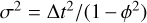 Following Vaughan et al. (2003), time bins are super-sampled forty-fold to avoid red noise leaks, and then summed. Finally, the random walk is normalised and mixed as a variable fraction fvar with a constant to obtain the source count rate as
  . The mean μ is varied in groups as in gaussvar, and five equally sized subgroups set fvar to 0.03,0.1, 0.2, 0.3, and 0.5, motivated by the range observed in X-ray binaries (Heil et al. 2015).
Simulating other types of variability, such as exponential or linear declines, sinusoidal variations are beyond the scope of this work. However, because almost all methods adopted here ignore the order of measurements, they are covered to some degree by the gaussvar setup.
To achieve accurate quantification of the methods, many simulations are needed. In total, 27 908 constant simulations (all eFEDS sources were used as templates), 14 003 gaussvar simulations (eFEDS sources with even IDs were templates), 13 905 flare simulations (eFEDS sources with odd IDs were templates), and 14 003 redvar simulations (same as gaussvar) were generated for the soft band. A similar number of simulations was performed for the hard band, but 28 light curves have no valid time bins and were discarded. We primarily focus on the soft-band simulations.
4 Results
4.1 Thresholds for low false-positive rates
To find a reliable threshold corresponding to a low false positive rate, the constant data set was used. The idea was to choose a threshold that rarely triggers in this non-variable data set and that it corresponds to some desired p-value. For a given method, its variability estimator was computed for each simulated constant light curve. This gives an estimator distribution for non-variable sources. Figures 11 and 12 show the distributions for the estimators of the maximum amplitude, excess variance, bexvar, and Bayesian blocks methods at various input count rates. The expectation is that because these are non-variable sources, a significance value as extreme as 3σ indeed occurs with a frequency (p-value) corresponding to 0.27%. However, Fig. 11 illustrates that the distribution of significance estimators (x-axis, in units of σ), does not exactly match the observed 2, 3, or 4σ quantiles of the distribution. This is because the significance estimators employ approximations such as Gaussian errors. For example, the normalised excess variance underestimates the significance: lσ significances almost never occur in data sets with <lcts/s. The amplitude maximum deviation also appears to slightly underestimate the significance (AMPL_SIG>2 is reached in fewer than 1% of cases). The deviations are most extreme in the low count-rate regime, where AMPL_SIG and NEV_SIG values never exceed 1 by chance.
We chose the threshold at the 3σ equivalent quantile of the distributions from Figs. 11 and 12. This corresponds to a 0.3% false-positive rate at that count rate. This approach can be applied to any estimators, whether it indicates a significance (like AMPL_SIG and NEV_SIG) or an effect size (like SCATT_LO and NBBLOCKS). Figure 13 shows these thresholds as a function of count rate. For excess variance (top panel of Fig. 13) and AMPL_SIG (middle panel), it lies in the 0-2σ range, and decreases towards low count rates. We recall that AMPL_MAX measures the distance between the lower error bar of the highest point and the upper error bar of the lowest point. When counts are low, the conservatively estimated error bars are large and mostly overlap, giving very low or negative AMPL_MAX values. The significance further judges the distance by the error bars. This causes AMPL_SIG to decrease with count rate and creates low numbers. A similar effect occurs with NEV_SIG due to the overly conservative error bars (see Sect. 3.1.1).
For the Bayesian excess variance, the SCATT_LO threshold has a peak and does not rise towards the extreme count rates (bottom panel of Fig. 13). The difference to AMPL_SIG and NEV_SIG may arise because SCATT_LO measures an effect size, not a significance. For Bayesian blocks, the significance threshold (bottom panel of Fig. 12) is always at ncp = 1. That is, when the Bayesian block splits the light curve, it is reliable.
To derive a significance threshold for use in practice, a count-rate distribution has to be assumed. Taking all simulations together would imply a log-uniform count-rate distribution. In reality, the source count rates peak between 0.1 and 1 cts/s and decline towards the high end approximately like a power law with index –1.5. To be conservative, we chose the highest threshold across the simulated count rates and present them in Table 1. Because the sample is dominated by faint sources, this leads to a lower false-positive rate than 3σ (0.3%), and thus fewer than the naively expected number of false positives (75 out of 27 910). We estimated the expected false-positive rate by weighting the simulations by a count-rate power law  . Table 1 lists the expected number of false positives in eFEDS for each method. For the Bayesian excess variance, the expected number is 12, for the other methods, essentially no outliers are expected. After choosing the significance threshold, we can now test which method is most sensitive to detect variability.
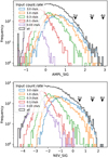 |
Fig. 11 Estimator distribution for simulated constant light curves. Top panel: amplitude maximum deviation significance (Eq. (9)). Bottom panel: significance of the excess variance and variability fraction (Eq. (16)). Each coloured histogram represents a set of simulations with the indicated constant input count rate. For the full data set (black histogram), black downward triangles point to the 2, 3, and 4σ equivalent quantiles of the distribution. |
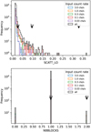 |
Fig. 12 As in Fig. 11, but for the bexvar SCATT_LO estimator (top panel), and the number of change points (NBBLOCKS) from the Bayesian blocks algorithm (bottom panel). In case of NBBLOCKS, the 3σ quantile is still within NBBLOCKS = 1. |
Reliable thresholds.
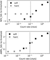 |
Fig. 13 Calibrated thresholds as a function of count rate. Points show the 3σ extreme for each simulation, for excess variance (top), amplitude maximum deviation (middle panel), and Bayesian excess variance (bottom panel). The vertical dotted line indicates the typical uncertainty on ṜS. |
4.2 Sensitivity evaluation
The goal of this section is to identify the correct variability method for detecting each type of variability. While the different methods are based on the same data (binned light curves), they vary in assumptions and how they use this information. Some ignore the order, and some ignore all but the most extreme points.
We quantified the sensitivity of each method using the gauss-var, redvar, and flare data sets. To do this, we applied the methods to each simulated light curve and computed the fraction above the significance thresholds calibrated in the previous section. This fraction is the completeness of the method. The simulations vary input count rate, strength, and type of variability, allowing an in-depth look at the behaviour of the different methods. This allowed us to characterise the detection efficiency by type (Fig. 14 for flare, Fig. 15 for gaussvar, and Fig. 16 for redvar), but also down to which k and σ values variability the methods are sensitive.
For flares (Fig. 14), amplitude maximum deviation and Bayesian excess variance are the most sensitive method. The amplitude maximum deviation performs better at very high count rates, while the Bayesian excess variance is most complete in all other situations. Flares of a factor of 5–10 are detectable for typical eROSITA sources with these methods. The normalised excess variance has comparable completeness as the Bayesian excess variance, except at the lowest count rates. Bayesian blocks is less efficient at all count rates.
For white-noise source variability from a log-normal distribution (Fig. 15), the Bayesian excess variance is the most sensitive method at all count rates, followed by the normalised excess variance, amplitude maximum deviation, and Bayesian blocks. In the more realistic red-noise scenario with a small variable fraction (Fig. 16), Bayesian excess variance also performs best in all but one simulation subgroup. Here, however, the Bayesian block algorithm performs similarly well. Overall, only large fractional variances (fvar ≥ 30%) in the high count-rate sources (ṜS > lcts/s) can be detected. To compare Figs. 15 and 16, σ ≈ fvar/2, if the random walk is well sampled.
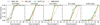 |
Fig. 14 Sensitivity of the methods to detecting flares. Panels represent simulations with increasing input count rates from left to right. Flares of varying strengths are injected (x-axis). The fraction of objects for which the method gives an estimate above the significance threshold is shown in the y-axis. At very high counts (left panels), the AMPL_SIG has the highest fraction. At medium and low counts, SCATT_LO has the highest detection fraction overall. |
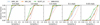 |
Fig. 15 As in Fig. 14, but for simulated white log-normal variability of varying strength σ (in dex). SCATT_LO has the highest detection fraction overall. |
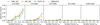 |
Fig. 16 As in Fig. 14, but for simulated red-noise variability of varying fraction fvar. Bayesian blocks has the highest detection fraction across all panels. |
5 Discussion and conclusion
This work focused on characterising four methods for detecting source variable X-ray sources. This includes the amplitude maximum deviation and Bayesian excess variance, normalised excess variance and Bayesian blocks.
5.1 Bexvar
The Bayesian excess variance (bexvar) is presented here for the first time. It is a fully Poissonian way to quantify source variability in the presence of background. We publish the bexvar code as free and open-source Python software3.
Currently, a simple time-independent log-normal distribution is assumed. However, the hierarchical Bayesian model is extensible. More complex variability models, such as fitting linear, exponentially declining, or periodic (sinosoidal) signals and potentially auto-regressive moving average processes (see e.g. Kelly et al. 2014) can be implemented and applied to Poisson data.
Employing the Bayesian excess variance as a method for detecting variability has some limitations. Requiring the 10% quantile on the log-normal scatter to exceed dex makes a cut on significance and effect size. This will not detect barely variable sources even when the data are excellent. Bayesian model comparison of a constant model to a log-normal model may be an even more powerful discriminator. The strength of the Bayesian excess variance is not in the detection of variability, but in variability quantification. In Appendix A we verify that the input parameters can be accurately and reliably retrieved.
5.2 Efficient detection of variable sources for eROSITA
When comparing the four methods, we find that each method has strengths in detecting certain types of variability. For flares, amplitude maximum deviation is both sensitive and simple to compute. It is optimised to detect single outliers, so it is not surprising that it performs well here. However, it is perhaps somewhat surprising that Bayesian excess variance performs similarly well. This may be because it models the Poisson variations carefully and is sensitive to excess variance. Both methods outperform the normalised excess variance and Bayesian blocks. We assume that carefully modelling the Poisson (source and background) noise leads to Bayesian excess variance outperforming the classical normalised excess variance.
For intrinsic log-normal variability, the Bayesian excess variance performs best overall. Comparing the panels in Fig. 15, it allows detecting variability in sources three times fainter than Bayesian blocks with Gaussian noise. This is expected, because it models the chosen simulated white noise process. At low count rates, it substantially outperforms the normalised excess variance, which assumes the same model but uses Gaussian approximations. It is surprising that amplitude maximum deviation also outperforms the normalised excess variance, even though the latter considers all points. However, the trends change when white noise is replaced with more realistic red noise. In this case, because data points are correlated in time, the order becomes important. Bayesian blocks, the only method tested here that takes the order of data points into account, performs better in this case. However, the detection efficiencies for realistic source parameters are very modest for all methods.
For observing patterns yielding only few (<20) light-curve data points, amplitude maximum deviation and Bayesian blocks are quick but effective methods and are therefore recommended for large surveys. The Bayesian excess variance requires more computational resources, but identifies a larger number of variable sources, especially in the low-count regime. This is demonstrated by our simulations, but it is also true in practice. All four presented methods were applied to the eFEDS observations in Boller et al. (2022) at the same false-positive rate (0.3%). The 65 sources significantly detected by one of the four methods primarily consist of flaring stars and variable active galactic nuclei. All methods were able to detect variability among the 2% brightest sources of the eFEDS sample. However, the Bayesian excess variance more than doubled the number of sources, and detects variability down to source count rates that encompass 20% of the eFEDS sample.
5.3 Outlook for the eROSITA all-sky survey
In some regards, the eFEDS survey investigated here has similar properties as the eROSITA all-sky survey (eRASS). eRASS will ultimately consist of eight all-sky scan. These scans take six months to complete. With the exception of sources near the ecliptic poles, which require different treatment (blue in Fig. 17), most sources are visited over a period of a few days and are covered repeatedly for a few minutes (orange in Fig. 17). This cadence pattern (3–8 chunks of observations, each resolved into multiple time bins) is similar to the eFEDS light curve cadence. The total exposure time of eFEDS is designed to be comparable to that of eRASS. Therefore, sources of similar count distributions are expected. Thus the simulation setup to test and compare variability methods, as well as the derived significance thresholds, have applicability also to the final eRASS observations.
In conclusion, we recommend the Bayesian excess variance and amplitude maximum deviation methods for the detection of variable sources in eROSITA, with the significance thresholds specified in Table 1. However, variability detection and characterisation methods benefit past, present, and future high-energy experiments. Improvements in method can lead to new discoveries in archival data and allow future mission such as Athena (Nandra et al. 2013) and the Einstein Probe (Yuan et al. 2015) to deliver more events in real time.
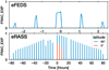 |
Fig. 17 Fractional exposure for an arbitrary eFEDS source (top panel) and two eRASS source at different ecliptic latitudes (bottompanel). |
Acknowledgements
We thank the anonymous referee for insightful comments that improved the paper. J.B. thanks Mirko Krumpe for comments on the manuscript. This work is based on data from eROSITA, the soft X-ray instrument aboard SRG, a joint Russian-German science mission supported by the Russian Space Agency (Roskosmos), in the interests of the Russian Academy of Sciences represented by its Space Research Institute (IKI), and the Deutsches Zentrum für Luft- und Raumfahrt (DLR). The SRG spacecraft was built by Lav-ochkin Association (NPOL) and its subcontractors, and is operated by NPOL with support from the Max Planck Institute for Extraterrestrial Physics (MPE). The development and construction of the eROSITA X-ray instrument was led by MPE, with contributions from the Dr. Karl Remeis Observatory Bamberg & ECAP (FAU Erlangen-Nuernberg), the University of Hamburg Observatory, the Leibniz Institute for Astrophysics Potsdam (AIP), and the Institute for Astronomy and Astrophysics of the University of Tübingen, with the support of DLR and the Max Planck Society. The Argelander Institute for Astronomy of the University of Bonn and the Ludwig Maximilians Universität Munich also participated in the science preparation for eROSITA. The eROSITA data shown here were processed using the eSASS/NRTA software system developed by the German eROSITA consortium. This work made use of the software packages matplotlib (Hunter 2007), UltraNest (https://johannesbuchner.github.io/UltraNest/) (Buchner 2021), astropy (https://www.astropy.org/) (Astropy Collaboration 2013, 2018), gammapy (https://gammapy.org/) (Deil et al. 2017; Nigro et al. 2019).
Appendix A Parameter recovery
While the focus of this work is on the detection of variability, some of the methods we employed quantify the variability. This depends on the assumed variability model, which are for example step functions in Bayesian blocks and (log) normal count rate scatter for the (Bayesian) excess variance. Based on the flare and white-noise simulations, the recovery of methods that closely resemble these signals are investigated.
Figure A.1 compares the injected log-variance to the inferred Bayesian excess variance in the gaussvar simulations. At all count rates and variability levels, the injected variance is correctly recovered.
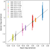 |
Fig. A.1 Inferred Bayesian excess variance for various simulated variances and count rates. Error bars indicate the 95% credible interval for an arbitrary subset of the simulations. A small displacement in the x-axis is added to each data point for clarity. The dotted line indicates the 1:1 correspondence. |
Figure A.2 compares the injected flare amplitude to the ampl_max measure. The distribution of values is indicated as a violin plot. Since ampl_max measures the span between error bars, it tends to conservatively underestimate the flare strength. Nevertheless, the overall correspondence is good.
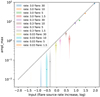 |
Fig. A.2 Inferred amplitude maximum deviation distribution (violin plots) for various input flare strengths. The dotted line indicates the 1:1 correspondence. Most ampl_max values typically lie below this line. |
References
- Armstrong, D. J., Kirk, J., Lam, K. W. F., et al. 2016, MNRAS, 456, 2260 [NASA ADS] [CrossRef] [Google Scholar]
- Astropy Collaboration (Robitaille, T. P., et al.) 2013, A&A, 558, A33 [NASA ADS] [CrossRef] [EDP Sciences] [Google Scholar]
- Astropy Collaboration (Price-Whelan, A. M., et al.) 2018, AJ, 156, 123 [Google Scholar]
- Bachetti, M., Harrison, F. A., Walton, D. J., et al. 2014, Nature, 514, 202 [NASA ADS] [CrossRef] [Google Scholar]
- Barlow, R. 2003, in Statistical Problems in Particle Physics, Astrophysics, and Cosmology, eds. L. Lyons, R. Mount, & R. Reitmeyer (Singapore: World Scientific), 250 [Google Scholar]
- Boller, T., Freyberg, M. J., Trümper, J., et al. 2016, A&A, 588, A103 [NASA ADS] [CrossRef] [EDP Sciences] [Google Scholar]
- Boller, T., Schmitt, J. H. M. M., Buchner, J., et al. 2022, A&A, 661, A8 (eROSITA EDR SI) [NASA ADS] [CrossRef] [EDP Sciences] [Google Scholar]
- Brunner, H., Liu, T., Lamer, G., et al. 2022, A&A, 661, A1 (eROSITA EDR SI) [NASA ADS] [CrossRef] [EDP Sciences] [Google Scholar]
- Buchner, J. 2016, Stat. Comput., 26, 383 [Google Scholar]
- Buchner, J. 2019, PASP, 131, 108005 [Google Scholar]
- Buchner, J. 2021, J. Open Source Softw., 6, 3001 [CrossRef] [Google Scholar]
- Cameron, E. 2011, PASA, 28, 128 [Google Scholar]
- Debosscher, J., Sarro, L. M., Aerts, C., et al. 2007, A&A, 475, 1159 [NASA ADS] [CrossRef] [EDP Sciences] [Google Scholar]
- Deil, C., Zanin, R., Lefaucheur, J., et al. 2017, Int. Cosmic Ray Conf., 301, 766 [Google Scholar]
- De Luca, A., Salvaterra, R., Belfiore, A., et al. 2021, A&A, 650, A167 [NASA ADS] [CrossRef] [EDP Sciences] [Google Scholar]
- Ducci, L., Ji, L., Haberl, F., et al. 2020, ATel, 11610, 13545 [Google Scholar]
- Edelson, R. A., Krolik, J. H., & Pike, G. F. 1990, ApJ, 359, 86 [NASA ADS] [CrossRef] [Google Scholar]
- Edelson, R., Turner, T. J., Pounds, K., et al. 2002, ApJ, 568, 610 [CrossRef] [Google Scholar]
- Gehrels, N. 1986, ApJ, 303, 336 [Google Scholar]
- Gehrels, N., & Mészáros, P. 2012, Science, 337, 932 [NASA ADS] [CrossRef] [Google Scholar]
- Gehrels, N., Chincarini, G., Giommi, P., et al. 2004, ApJ, 611, 1005 [Google Scholar]
- Heil, L. M., Uttley, P., & Klein-Wolt, M. 2015, MNRAS, 448, 3348 [Google Scholar]
- Heinze, A. N., Tonry, J. L., Denneau, L., et al. 2018, AJ, 156, 241 [Google Scholar]
- Holl, B., Audard, M., Nienartowicz, K., et al. 2018, A&A, 618, A30 [NASA ADS] [CrossRef] [EDP Sciences] [Google Scholar]
- Hunter, J. D. 2007, Comput. Sci. Eng., 9, 90 [NASA ADS] [CrossRef] [Google Scholar]
- Jayasinghe, T., Stanek, K. Z., Kochanek, C. S., et al. 2019, MNRAS, 486, 1907 [NASA ADS] [Google Scholar]
- Kelly, B. C., Becker, A. C., Sobolewska, M., Siemiginowska, A., & Uttley, P. 2014, ApJ, 788, 33 [NASA ADS] [CrossRef] [Google Scholar]
- Kim, D.-W., Protopapas, P., Byun, Y.-I., et al. 2011, ApJ, 735, 68 [NASA ADS] [CrossRef] [Google Scholar]
- Klebesadel, R. W., Strong, I. B., & Olson, R. A. 1973, ApJ, 182, L85 [NASA ADS] [CrossRef] [Google Scholar]
- Knoetig, M. L. 2014, ApJ, 790, 106 [NASA ADS] [CrossRef] [Google Scholar]
- Koenig, O., Wilms, J., Kreykenbohm, I., et al. 2020, ATel, 13765 [Google Scholar]
- Kraft, R. P., Burrows, D. N., & Nousek, J. A. 1991, ApJ, 374, 344 [Google Scholar]
- Liu, J.-F., Bregman, J. N., Bai, Y., Justham, S., & Crowther, P. 2013, Nature, 503, 500 [NASA ADS] [CrossRef] [Google Scholar]
- Liu, T., Buchner, J., Nandra, K., et al. 2022, A&A, 661, A5 (eROSITA EDR SI) [NASA ADS] [CrossRef] [EDP Sciences] [Google Scholar]
- Lorimer, D. R., Bailes, M., McLaughlin, M. A., Narkevic, D. J., & Crawford, F. 2007, Science, 318, 777 [Google Scholar]
- Malyali, A., Rau, A., Merloni, A., et al. 2021, A&A, 647, A9 [NASA ADS] [CrossRef] [EDP Sciences] [Google Scholar]
- Masci, F. J., Hoffman, D. I., Grillmair, C. J., & Cutri, R. M. 2014, AJ, 148, 21 [NASA ADS] [CrossRef] [Google Scholar]
- Matsuoka, M., Kawasaki, K., Ueno, S., et al. 2009, PASJ, 61, 999 [Google Scholar]
- Maughan, B. J., & Reiprich, T. H. 2019, Open J. Astrophys., 2, 9 [Google Scholar]
- Miniutti, G., Saxton, R. D., Giustini, M., et al. 2019, Nature, 573, 381 [Google Scholar]
- Nandra, K., George, I. M., Mushotzky, R. F., Turner, T. J., & Yaqoob, T. 1997, ApJ, 476, 70 [Google Scholar]
- Nandra, K., Barret, D., Barcons, X., et al. 2013, ArXiv e-prints [arXiv:1306.2307] [Google Scholar]
- Nigro, C., Deil, C., Zanin, R., et al. 2019, A&A, 625, A10 [NASA ADS] [CrossRef] [EDP Sciences] [Google Scholar]
- Palaversa, L., Ivezić, Ž., Eyer, L., et al. 2013, AJ, 146, 101 [CrossRef] [Google Scholar]
- Petroff, E., Hessels, J. W. T., & Lorimer, D. R. 2019, A&ARv, 27, 4 [NASA ADS] [CrossRef] [Google Scholar]
- Ponti, G., Munoz-Darias, T., & Fender, R.P. 2014, MNRAS, 444, 1829 [NASA ADS] [CrossRef] [Google Scholar]
- Predehl, P., Andritschke, R., Arefiev, V., et al. 2021, A&A, 647, A1 [EDP Sciences] [Google Scholar]
- Scargle, J. D., Norris, J. P., Jackson, B., & Chiang, J. 2013, ApJ, 764, 167 [Google Scholar]
- Simm, T., Salvato, M., Saglia, R., et al. 2016, A&A, 585, A129 [NASA ADS] [CrossRef] [EDP Sciences] [Google Scholar]
- Swank, J. H. 2006, Adv. Space Res., 38, 2959 [NASA ADS] [CrossRef] [Google Scholar]
- van Roestel, J., Duev, D. A., Mahabal, A. A., et al. 2021, AJ, 161, 267 [NASA ADS] [CrossRef] [Google Scholar]
- Vaughan, S., Edelson, R., Warwick, R. S., & Uttley, P. 2003, MNRAS, 345, 1271 [Google Scholar]
- Weber, P. 2020, GRB Coordinates Network, 26988, 1 [NASA ADS] [Google Scholar]
- Wilms, J., Kreykenbohm, I., Weber, P., et al. 2020, ATel, 13416 [Google Scholar]
- Yuan, W., Zhang, C., Feng, H., et al. 2015, ArXiv e-prints [arXiv:1506.07735] [Google Scholar]
All Tables
All Figures
|
Fig. 1 Example counts of the tenth brightest eFEDS source. The markers indicate the number of counts from a single eROSITA telescope module in 100s time bins, recorded over a six-hour period. The black curve shows the sensitivity to the source position over time. |
| In the text | |
|
Fig. 2 Distribution of fractional exposure (fexpo) values for all light-curve time bins. |
| In the text | |
|
Fig. 3 Light-curve cadence summary statistics. Top panel: the time between first and last exposed time bins for each light curve, with typical values of four to seven hours. As Fig. 1 illustrates, the light curves are segmented into blocks. Middle panel: number of blocks, which ranges from 4 to 12. Bottom panel: duration of the longest block for each light curve, which typically lasts only a few minutes. |
| In the text | |
|
Fig. 4 Source and background photon-count distribution in the soft and hard bands. The background counts are scaled by the ratio of source to background area. |
| In the text | |
|
Fig. 5 Visualisations. Top panel: fractional exposure over time for an example source with 10 passes. Bottom panel: light curve of a simulated source with constant count rate and a bright flare. Black circles show the total counts without background subtraction, and red points show the expected background count rates in the source region (Eq. (4)). Grey error bars show classical net source count-rate estimates (Eqs. (3) and (5)). Black error bars show Bayesian net source count-rate posterior distributions, represented visually with 10, 50, and 90% quantiles under a log-uniform prior (Eq. (7)). |
| In the text | |
|
Fig. 6 Cumulative count visualisation. The red curve shows the observed cumulative counts over time. The expectation of a constant source is indicated as a dashed curve and grey intervals corresponding to 1, 2, and 3σ. |
| In the text | |
|
Fig. 7 Graphical model of the Bayesian excess variance method. Shaded circles indicate known values, related to the experiment setup or observed data. Rectangles indicate unknown parameters, including the unknown source count rate and the count rate in each time bin. An arrow from A to B indicates that the generation of B was influenced by A. |
| In the text | |
|
Fig. 8 Simulated light curves of constant sources with Poisson noise. Black circles show the total counts without background subtraction, and red points show the expected background count rates in the source region (Eq. (4)). Top panel: source with a high count rate with a constant 3 cts/s, where the source counts are always above the expected background counts. Bottom panel: source with a low count rate with a constant 0.03 cts/s, where source region counts and background counts are comparable and show substantial Poisson scatter. Grey error bars show classical net source count-rate estimates (Eqs. (3) and 5). Black error bars show Bayesian net source count-rate posterior distributions (Eq. (7)). |
| In the text | |
|
Fig. 9 As in Fig. 8, but for gaussvar sources. The intrinsic count rate is randomly varied following a log-normal distribution around a baseline count rate. Left panels: cases with σ = 1dex variations, clearly visible in the scatter of the total counts (black points) in both bright (top panel) and faint (bottom panel) sources. Right panels: lower variations (σ = 0.1 dex). In the bright case (top panel), the scatter of the black points is substantially larger than the error bars, while in the faint case (bottom), the error bars overlap. In the top panel the background contribution (red points) is well below the total counts (black), while in the bottom panel, they are comparable. The solid blue line and band show the posterior median and 1a uncertainty of the intrinsic source count rate |
| In the text | |
|
Fig. 10 As in Fig. 9, but for flare sources. The count rate in one bin is increased by a factor of k. The top (bottom) panels: bright (faint) source baseline count rates. Top panels: flare of k = 10, and bottom panels: k = 2 flare. |
| In the text | |
|
Fig. 11 Estimator distribution for simulated constant light curves. Top panel: amplitude maximum deviation significance (Eq. (9)). Bottom panel: significance of the excess variance and variability fraction (Eq. (16)). Each coloured histogram represents a set of simulations with the indicated constant input count rate. For the full data set (black histogram), black downward triangles point to the 2, 3, and 4σ equivalent quantiles of the distribution. |
| In the text | |
|
Fig. 12 As in Fig. 11, but for the bexvar SCATT_LO estimator (top panel), and the number of change points (NBBLOCKS) from the Bayesian blocks algorithm (bottom panel). In case of NBBLOCKS, the 3σ quantile is still within NBBLOCKS = 1. |
| In the text | |
|
Fig. 13 Calibrated thresholds as a function of count rate. Points show the 3σ extreme for each simulation, for excess variance (top), amplitude maximum deviation (middle panel), and Bayesian excess variance (bottom panel). The vertical dotted line indicates the typical uncertainty on ṜS. |
| In the text | |
|
Fig. 14 Sensitivity of the methods to detecting flares. Panels represent simulations with increasing input count rates from left to right. Flares of varying strengths are injected (x-axis). The fraction of objects for which the method gives an estimate above the significance threshold is shown in the y-axis. At very high counts (left panels), the AMPL_SIG has the highest fraction. At medium and low counts, SCATT_LO has the highest detection fraction overall. |
| In the text | |
|
Fig. 15 As in Fig. 14, but for simulated white log-normal variability of varying strength σ (in dex). SCATT_LO has the highest detection fraction overall. |
| In the text | |
|
Fig. 16 As in Fig. 14, but for simulated red-noise variability of varying fraction fvar. Bayesian blocks has the highest detection fraction across all panels. |
| In the text | |
|
Fig. 17 Fractional exposure for an arbitrary eFEDS source (top panel) and two eRASS source at different ecliptic latitudes (bottompanel). |
| In the text | |
|
Fig. A.1 Inferred Bayesian excess variance for various simulated variances and count rates. Error bars indicate the 95% credible interval for an arbitrary subset of the simulations. A small displacement in the x-axis is added to each data point for clarity. The dotted line indicates the 1:1 correspondence. |
| In the text | |
|
Fig. A.2 Inferred amplitude maximum deviation distribution (violin plots) for various input flare strengths. The dotted line indicates the 1:1 correspondence. Most ampl_max values typically lie below this line. |
| In the text | |
Current usage metrics show cumulative count of Article Views (full-text article views including HTML views, PDF and ePub downloads, according to the available data) and Abstracts Views on Vision4Press platform.
Data correspond to usage on the plateform after 2015. The current usage metrics is available 48-96 hours after online publication and is updated daily on week days.
Initial download of the metrics may take a while.