| Issue |
A&A
Volume 661, May 2022
The Early Data Release of eROSITA and Mikhail Pavlinsky ART-XC on the SRG mission
|
|
|---|---|---|
| Article Number | A8 | |
| Number of page(s) | 13 | |
| Section | Catalogs and data | |
| DOI | https://doi.org/10.1051/0004-6361/202141155 | |
| Published online | 18 May 2022 | |
The eROSITA Final Equatorial-Depth Survey (eFEDS)
Variability catalogue and multi-epoch comparison★
1
Max-Planck-Institut für extraterrestrische Physik,
Giessenbachstrasse 1,
85748
Garching, Germany
e-mail: This email address is being protected from spambots. You need JavaScript enabled to view it.
2
Hamburger Sternwarte, Universität Hamburg,
Gojenbergsweg 112,
21029
Hamburg, Germany
3
National Observatory of Athens, I. Metaxa & V. Pavlou, P. Penteli,
15236
Athens, Greece
4
Leibniz-Institut für Astrophysik Potsdam (AIP),
An der Sternwarte 16,
14482
Potsdam, Germany
Received:
21
April
2021
Accepted:
21
June
2021
Abstract
The 140-square-degrees Final Equatorial-Depth Survey (eFEDS) field, observed with the extended ROentgen Survey with an Imaging Telescope Array (eROSITA) on board the Spectrum-Roentgen-Gamma mission, provides a first look at the variable eROSITA sky. We analysed the intrinsic X-ray variability of the eFEDS sources and provide X-ray light curves and tables with variability test results in the 0.2–2.3 keV (soft) and 2.3–5.0 keV (hard) bands. We performed variability tests using the traditional normalised excess variance and maximum amplitude variability methods (as performed for the 2RXS catalogue), and we present results from the Bayesian excess variance and Bayesian block methods. We identified 65 sources as being significantly variable in the soft band. In the hard band, only one source is found to vary significantly. For the most variable sources, the light curves are well fit by an empirical stellar flare model and reveal extreme flare properties. A few highly variable active galactic nuclei have also been detected. About half of the variable eFEDS sources are detected in the X-rays for the first time with eROSITA. Comparison with 2RXS and XMM-Newton observations provides variability information on timescales of years to decades.
Key words: X-rays: general / line: formation / surveys
Table of the eFEDS sources with variability test results is only available at the CDS via anonymous ftp to cdsarc.u-strasbg.fr (130.79.128.5) or via http://cdsarc.u-strasbg.fr/viz-bin/cat/J/A+A/661/A8
© Th. Boller et al. 2022
 Open Access article, published by EDP Sciences, under the terms of the Creative Commons Attribution License (https://creativecommons.org/licenses/by/4.0), which permits unrestricted use, distribution, and reproduction in any medium, provided the original work is properly cited.
Open Access funding provided by Max Planck Society.
1 Introduction
Variability is a ubiquitous and defining characteristic of coronal stellar and accreting compact object systems, which represent two main object classes of variable X-ray sources. Typically, the most rapid variations with the largest amplitude are observed in the X-ray band, suggesting that in stars, the X-rays originate from magnetic reconnection processes. For accreting systems, the X-rays must arise very close to the compact object, as do the processes that cause the variability. Observational studies of stellar X-ray activity and of accreting supermassive black hole systems have revealed a rich phenomenology in terms of observations and associated theoretical models to explain them.
The eROSITA Final Equatorial-Depth Survey (eFEDS) field was observed in November 2019 with the extended ROentgen Survey with an Imaging Telescope Array (eROSITA) on board the Spectrum-Roentgen-Gamma (SRG) mission (SRG/eROSITA; Predehl et al. 2021) as part of its performance verification programme. These observations were performed in field-scan mode. Further details and a catalogue of X-ray sources can be found in Brunner et al. (2022). The eFEDS observations provide a deep view of the X-ray variability over an unprecedentedly large contiguous field of about 140 square degrees on timescales from seconds to hours, and even longer timescales when compared to previous observations by other X-ray observatories. For example, a comparison of eFEDS sources with XMM-Newton observations provides information on source variability on timescales of years. The 2RXS catalogue (Boller et al. 2016) contains detailed variability information from an even earlier epoch (1990–1991), which is useful for comparisons with the timing properties of sources detected in the eFEDS field.
2 Observations and data preparation
The eFEDS field scan rate is 0.003654 degs−1, roughly 1/7 of the all-sky survey scan rate of eROSITA. The resulting field-of-view (FOV) crossing time of any given source is about 300 s, and each position is covered again after typically about 2000 s. Three consecutive visits are typically made over locations within the body of the survey area. For sources at the eFEDS field borders, there are scan reversals and more than three consecutive visits are available because these sources cross the FOV twice. The total elapsed time from the first to the last observation of a source is up to about 22 000 s; the precise temporal sampling depends on the position within the field.
The eFEDS survey scanning strategy is especially sensitive to stellar flaring events, which have decay times of about a few thousand seconds. This can be compared to the eROSITA all-sky survey mode, wherein any single sky location is typically observed for about seven passes per season, each pass separated by about 14 000 s, followed by a long gap (about 6 months) between seasons. The number of passes per season is dependent on the location of a source in the sky. The eFEDS data also differ from the ROSAT all-sky survey, in which data points were obtained every 5760 s for approximately two days.
The eFEDS event file was processed and cleaned as described in Brunner et al. (2022). We extracted light curves from the cleaned event file for all 27910 sources in the eFEDS main X-ray catalogue (Brunner et al. 2022) using the eROSITA Science Analysis Software System (eSASS) task srctool1 (Version 1.63; Brunner et al. 2022). The source extraction region was chosen as a circular region that maximizes the signal-to-noise ratio of the source. The background extraction region is an annular region that is 200 times larger than the source extraction region. Contamination from nearby sources was excluded from the source and background regions. More details about the regions are described in Liu et al. (2022), who used the same regions to extract the X-ray spectra. With these regions as input to srctool, we extracted the light curves in the (0.2–5), (0.2–2.3), and (2.3–5) keV bands, including all valid event patterns (PATTERN <= 15), and a adopting time bin size of ∆t = 100 s. The srctool software measures the background counts B, source counts S, the scaling factor r between the source and background regions, and then calculates the net source count rate Xi in each time bin i as

The effective exposure fraction fexp was calculated to account for the instrumental factors that affect the source photon counts in each time bin and each energy band at a given source count rate. The product of the fraction of the time bin overlaps the input good time intervals (GTIs) and the fraction of the nominal effective collecting area seen by the source. The latter accounts for several effects: the local telescope vignetting, the flux loss caused by flagged bad pixels, the boundary of the instrumental FOV, and the flux lost outside the source extraction region due to the instrumental point spread function (PSF). In general, the srctool software uses the total counts in the source and background regions to estimate the count rate errors as the square root of the counts. In the cases of low counts per bin (<25), this estimator becomes inaccurate, and thus no error estimate is provided by srctool. In these cases, we estimated the error on the counts as  (Gehrels 1986). This is important because otherwise these time bins would have been excluded from the variability analysis, which would have biased the analysis.
3 Method
3.1 eROSITA variability tests
In the following we analyse the variability properties of the eFEDS point sources. In each of the three energy bands, four different variability characterisation methods are applied. These include the normalised excess variance (NEV) (Edelson et al. 1990, 2002; Nandra et al. 1997), maximum amplitude variability (Boller et al. 2016), Bayesian blocks (Scargle et al. 2013), and the Bayesian excess variance (Buchner et al. 2022). These tests are presented in detail in Buchner et al. (2022), who also studied their performance for an eFEDS-like survey in detail. Here, we briefly introduce each method.
3.1.1 Maximum amplitude variability
The maximum amplitude variability is defined as the span between the most extreme values of the count rate,
 (1)
(1)
where Xmax (Хmin) is the maximum (minimum) count rate and the associated error is σmax (σmin). The uncertainty is
 (2)
(2)
The ratio ampl_max to σ(ampl_max) gives the significance of the maximum amplitude variability in units of σ. Buchner et al. (2022) identified with simulations that at a threshold of ampl_max/σ(ampl_max) > 2.6 we expect no false positives in an eFEDS-like field. The definition of ampl_max is a conservative lower limit on the variability and follows its original definition in Boller et al. (2016).
3.1.2 Excess variability estimators
The NEV is defined as the difference between the expected variance from the error bars σi and the observed variance,
 (3)
(3)
The NEV estimator does not have an analytic uncertainty. Vaughan et al. (2003) performed extensive numerical studies and found the empirical formula
 (4)
(4)
where μ is the mean count rate, σi are the count rate uncertainties, and  is the mean of the square of the count rate uncertainties. N is the number of data points. The fractional variability Fvar (Edelson et al. 1990) is simply the square root of the NEV defined by Nandra et al. (1997). The ratio of NEV and σ(NEV) gives the significance of the normalised excess variance in units of σ. The simulations of Buchner et al. (2022) suggest that a threshold of NEV/σ(NEV))1.7 is appropriate if we wish to avoid false positives in an eFEDS-like field.
The assumption of Gaussianity in the calculation of the NEV breaks down in the low count rate regime. Buchner et al. (2022) therefore developed a Bayesian excess variance estimate (bexvar) that works with the Poisson counts instead of inferred uncertainties. For the source variability, the Bayesian excess variance model assumes a log-normal distribution for the counts and infers its variance  . We used the bexvar Python implementation2, which computes posterior probability distributions using the nested-sampling inference algorithm MLFriends (Buchner 2014, 2019) implemented in the UltraNest Python package3 (Buchner 2021). Buchner et al. (2022) reported that a threshold of 0.14 dex on the lower 10% quantile of σbexvar has fewer than 0.3% false positives in eFEDS-like simulated light curves. The log-normal assumption is a simple distribution, which is guaranteed to always produce positive count rates (unlike e.g. a normal distribution). Given the few data points per source (approximately 20) and the low counts in all but a few sources, it is difficult to estimate higher moments than the variance.
3.1.3 Bayesian blocks
The Bayesian blocks algorithm (Scargle et al. 2013) breaks light curves into segments with constant count rates. Starting from the first data point, every iteration of the algorithm adds one data point at a time, making use of stored results of previous iteration to obtain a new exact optimum at each step. The result is the exact global optimum in time of order N2 (which would be impossible with an explicit search of the exponential search space − 2N in size). In effect, it yields the step-function that optimally fits the data of all possible such representations. Variability is detected with this method when the algorithm breaks the light curve into at least two segments.
Bayesian blocks can be directly applied to photon counts and do not require binning. However, Bayesian blocks applied in this way could detect variability caused by the varying sensitivity and background. This is because the permanently changing orientation of eROSITA modulates the count rates from the source and some components of the background, which can dominate the signal. To measure the source flux variability (instead of the observed count rate variability), the background and instrument sensitivity at any time needs to be incorporated. While the original count event formulation of Bayesian blocks can incorporate varying sensitivity, contributions from a potentially varying background deduced by an ‘off’ region go beyond the current work (but see Kerr 2019, for Bayesian blocks extensions) However, when the Gaussian approximation is used in a pre-binned light curve, we can infer the (background-corrected) source count rate at each time bin, (Xi, σi). The Bayesian block formulation using the Gaussian error bars can then attempt to detect changes. When these Gaussian Bayesian blocks are applied to eFEDS-like simulations (Buchner et al. 2022), it was found that this method produces virtually no false positives. We used the Bayesian blocks implementation from astropy (Astropy Collaboration 2013, 2018)4.
3.2 Comparison of variability test methods
Generally speaking, NEV tests for variability over the length of the observation, and it is sensitive to variability trends on these timescales. Maximum amplitude variability is used to search for flaring events based on the highest and lowest data points. Bayesian blocks and Bayesian excess variance are in addition sensitive to variability on timescales longer than 100 s and in the lower count rate regime.
3.3 Optical contamination by bright stars
Bright stars with Gaia G < 4.5 mag that are detected exclusively in the soft band are likely to be particularly problematic. The recorded signal is frequently optically contaminated. These stars cause apparent variability and trigger false positives. They were therefore removed from the sample. In a companion paper (Schmitt et al. 2021), the issue of optical contamination is discussed in detail.
3.4 Visualisations
We employed two visualisations to enable visual inspection of potentially interesting light curves. Firstly, the time series of Xi was plotted with error bars, allowing the identification of strong trends and bright flares. However, because most bins contain few counts and the error bars are accordingly large, it is difficult to accumulate evidence of adjacent bins. Therefore we also used a plot of the cumulative total counts and compared it to the expectation from a constant source with the same net count rate under the same observing conditions. We classify sources as described below.
Non-candidates are sources in which no variability test is triggered. These are the vast majority and are not presented here. Potential light leak false positives trigger a test, but there is a bright (G < 4.5) Gaia source in the close vicinity. Likely variables trigger a test, but the visual inspection of the cumulative counts does not exceed the 2σ range in any time bin. Secure variables trigger a test and the visual inspection of the cumulative counts exceeds the 2σ range in some time bin.
The vast majority of eROSITA point sources are either AGN or coronally active stars, and hence they are likely to be intrinsically variable. Here we report only the sources in which we can detect significant variability based on the eFEDS observations. This highlights the sources that were most strongly variable during the observation period.
4 Results
4.1 Variability test results
For all eFEDS sources we calculated the normalised excess variability, the maximum amplitude variability, the Bayesian excess variability, and the Bayesian blocks values and then tested these against the significance thresholds obtained by Buchner et al. (2022). In the soft (0.2–2.3) keV band, we find 80 sources for which at least one of the four variability tests results in a significant variability detection. In Fig. 1 we show the distribution of these sources in average count rate and ampl_max; in the low count-rate regime, only bexvar identifies variable sources, while most sources identified by NEV and ampl_max are also identified by other tests.
The NEV and ampl_max methods provide reliable variability test results in the high count-rate regime and test variability on timescales longer than the 100-s binning. In addition, the Bayesian excess variance and the Bayesian block method also select variable sources at lower count rates. To validate the significances (especially in the low count-rate regime), we applied a validation method by comparing the observed counts with the simulated counts for a constant source. We considered a source as variable when the number of observed counts was higher than 3σ compared to the constant count rate for in at least one time bin. These methods test variability on timescales longer than the FOV crossing time by merging data points between separate scans over sources. Applying the 3σ count criterion, we find reliable variability in the (0.2–2.3) keV energy band for 65 out of the 80 selected sources. In Fig. 2 we show the light curves and the cumulative count plots for one source in the high count-rate regime (ID 2) and for one fainter source (ID 837) as an example for variability in the low count-rate regime. In the hard (2.3–5.0 keV) band, only source ID 2 is found to be significantly variable based according to the Bayesian excess variance test. This source is also variable in the soft band. To give an impression of the obtained light curves, we show in Fig. 3 the 12 most variable sources in our variability search.
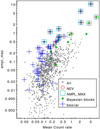 |
Fig. 1 Sample distribution in mean count rate and ampl_max. For each test, the sources considered significantly variable are marked. While most of these markers are limited to the upper left corner, the blue crosses extend to the bottom left corner of the plot. This reflects the sensitivity of bexvar in the low count-rate regime. |
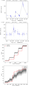 |
Fig. 2 Light curves (top two panels) and cumulative count plots (lower two panels) for two eFEDS sources (source IDs 2 and 837). The grey shadowed areas in the cumulative plots indicate count rate deviations of 1, 2, and 3σ with respect to a constant count rate per cumulative time bin. |
4.2 Most variable eFEDS sources
In Table 1 we list the most variable objects that passed at least one of the significance threshold tests, ordered by descending maximum amplitude variability in terms of σ. We adopted the most likely optical counterpart identifications from Salvato et al. (2022). The vast majority of the counterparts to the highly variable X-ray sources show significant Gaia parallaxes or proper motions, indicating that they are secure Galactic objects (following the same classification scheme as used by Salvato et al. 2022). The spectral type of the stellar counterpart is also shown in the Table, based on publicly available spectra. Four objects in this table are classified as extragalactic (based again on the Salvato et al. 2022 criteria), and we list the AGN classification type where available. Potential light leak false positives (with Gaia G < 4.5 mag that are detected exclusively in the soft band) were removed from the sample. Table 1 shows that the great majority of the variable sources are of Galactic origin. Most of the Galactic counterparts are stars of spectral type K and M; this is in line with very similar findings in the variability study in the ROSAT all-sky survey reported by Fuhrmeister & Schmitt (2003). In the following we present more detailed investigations of individual sources and comparisons to related studies.
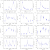 |
Fig. 3 Light curves for the 12 most variable eFEDS sources. The bin size is 100 s and the energy band is band 1. The objects are ordered from top left to right bottom in descending maximum amplitude σ values. For the normalized excess variance and the maximum amplitude variability the values in units of σ are indicated along the top of each panel. The variability flags (T for true and F for false) are also listed for the Bayesian excess variance (bexvar), and the Bayesian block method (nblocks). |
4.3 Stellar flare events
Because of the scanning character of the eFEDS observations of eROSITA, the detected X-ray sources are not covered continuously. This creates a problem for stellar flares because important parameters such as the time of flare onset and the time and amplitude of flare peak and flare decay may be missed or may be sampled only partially. Clearly, if there is only one high data point in a light curve, we can note that a flare most likely occurred, but little or nothing can be inferred about the flare energetics. By visual inspection, we identified six stellar flares (cf. Table 2) with sufficient X-ray coverage to allow a meaningful characterisation of the flares.
To describe the flares, we used an empirical ad hoc model, assuming a constant coronal background B, interpreted as the quiescent X-ray luminosity, a linear increase from the time of flare onset (tonset) to the time of flare peak (tpeak) with some flare amplitude A, followed by an exponential decay with some characteristic timescale tdecay, hence the model is defined by five adjustable parameters. This phenomenological model is clearly quite simplistic, but many (but not all) stellar flares can be reasonably well described by this ansatz. The X-ray light curves together with our fits are presented in Fig. 4; formally, all our fits are statistically acceptable.
Even then there may be remaining ambiguities depending on how the light curve was sampled. The time of flare onset is usually not observed, and given the scanning character of our observations, the time of flare peak and hence the peak amplitude are often also not observed. Whilst the former is not that relevant for the overall flare energetics (only a small fraction of the X-ray energy is radiated away in the rise phase), the total energy in the decay phase is directly proportional to the typically unobserved flare amplitude. We therefore attempted to construct minimum energy models, that is, models that would yield the lowest peak X-ray luminosities and lowest X-ray energies whilst still describing the observations. Our numbers should therefore be considered lower limits.
In Table 2 we list the sources that we analysed in detail and the derived flare parameters. We specifically provide the source ID, the inferred bolometric luminosities (in solar units), the measured quiescent X-ray luminosities, the derived decay timescale, observed peak X-ray luminosities and total X-ray energies, as well as the LX/Lbol ratios with respect to the quiescent and peak X-ray luminosities; the X-ray parameters are derived in this paper, and the bolometric luminosities were computed from the tables provided by Pecaut & Mamajek (2013). Two of the flaring stars listed in Table 2 are actually visual binaries that cannot be separated by eROSITA, and hence the flare site is unknown. Source ID 2 (= TYC 211-1502-1) consists of a K-type star and an M-type star at the same distance, but separated by 3.2″, and source ID 5 (=HD 79873) consists of an F-type and a later-type companion at an angular distance of 2.4″. The remaining host stars appear to be single (using Gaia EDR3). Inspecting the decay timescales listed in Table 2, we note that in most cases, the decay times are short (500–2000 s). During the eFEDS observations, sources were typically exposed for 400 s per scan, so that these decay times are usually reasonably well defined. Only the flare(s) observed on HD 79873 lasted longer; the long-duration flare of HD 79873 appears to consist of two individual events with much longer decay timescales.
The flares observed for source ID 77 (Gaia EDR3 3851068578984344448), ID 95 (Gaia EDR3 3841081371271550080), and ID 413 (Gaia EDR3 3074574363434013824) are of special interest. All of these flares are observed from apparently unremarkable stars, although all three stars are very red and very faint (cf. Gaia G magnitudes and BP-RP colours listed in Table 1). The eROSITA and Gaia positions agree very well, and at least no other Gaia sources are located in the vicinity. The flares observed by eROSITA, which are qualitatively similar to canonical stellar flares, therefore make our identifications unequivocal. ID 95 appears to be outstanding; according to Gaia, it is located at a distance of 308 pc with an uncertainty of about 10 pc, consequently, its quiescent and flaring X-ray luminosities are quite high.
The ratio of the observed peak X-ray luminosity and the quiescent bolometric luminosity approaches unity for ID 77 and ID 95. Observations of late-type dwarfs with Kepler and TESS have demonstrated that flares on late-type stars can produce significant enhancements even in their broadband optical light curves, that is, in the case of TESS, in the band between 6000 and 10000 Å. Ground-based flare observations are typically carried out in the U or B bands. The most extreme event in the study of TESS-observed optical flares reported by Günther et al. (2020) occurred on the M 4.5 star Gaia EDR3 5495481200071568640/2MASS J06270005-5622041, which increased its optical flux (in the TESS band) by a factor of 16.1 with a total energy release of 1034.7 erg. With its colour of BP-RP = 2.98, it is quite similar to the stars considered here. Schmitt et al. (2019) analysed TESS and XMM-Newton flare observations of the young active star AB Dor (spectral type K0) and demonstrated that the optical output of these flares is likely of the order of the X-ray output and possibly higher by up to one order of magnitude. In this context, we note that the total energy output of our most extreme X-ray event (from ID 95) coincides nicely with that obtained for Gaia EDR3 5495481200071568640 in the optical.
The highest ratios of the observed peak X-ray luminosity and the quiescent bolometric luminosity approaches that are reasonable can be determined as follows. We consider an M dwarf with Teff = 3000 K and a peak flare X-ray flux of 1031 erg s−1, and assume that during the flare Teff,flare = 12000 K, which is a typical chromospheric temperature, and Lopt,flare = LX,flare = 1031 erg s−1. Under these assumptions, a flare area smaller than 1% of the stellar surface would be sufficient to lead to Lstar,flare = Lstar,quiet, and coverage fractions of a few percent would be required to account for extreme cases such as Gaia EDR3 5495481200071568640/2MASS J06270005-5622041. Incidentally, Gaia EDR3 5495481200071568640/2MASS J06270005-5622041 is seen as a saturated X-ray source in eRASS1 with log(LX,quiet/Lbol,quiet) = −2.45 and is likely to produce X-ray flares similar to those described here.
Most variable eFEDS sources in the energy band (0.2–2.3) keV ordered in descending maximum amplitude values.
eFEDS sample of stellar flares.
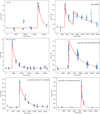 |
Fig. 4 Fits to stellar flares for objects in Table 1 with source identifications 2, 5, 6, 77, 95, and 413 (from top left to bottom right). |
4.4 Remarks on the AGN sub-sample
The majority of the discovered intrinsically variable sources are classified as secure Galactic or likely Galactic according to Salvato et al. (2022). Only 18% are of extragalactic origin. Three objects are classified as Seyfert 1 galaxies (Mrk 707, 2MASX J08561784-0138073, and 2MASS J08402550+0333018). All of these objects have been detected in the 2RXS catalogue (Boller et al. 2016). Four objects are classified as QSOs (SDSS J091000.01+034429.1, [VV2006] J085141.5+011930, [VV2006] J091637.5+004734, and [VV2006] J092346.8+011142). Only the last object has an 3XMM X-ray detection. Three objects are classified as galaxies (SDSS J090905.13+010929.6, SDSSCGB 12543.2, and TXS 0929+017). None of these sources have been detected with previous X-ray missions. Two objects are identified as the brightest cluster galaxy (BCG). These are SDSS J084150.93-001540.7 and SDSS J083125.18+034333.1, and are detected in X-rays for the first time with eROSITA.
5 Comparison with 2RXS
We cross-correlated the 2RXS catalogue (Boller et al. 2016) with the eFEDS main catalogue by searching for the nearest eFEDS source within 30″ of any 2RXS source. We matched 322 2RXS sources to 359 eFEDS sources in this way. Figure 5 (left panel) compares the eFEDS 0.2–2.3 keV count rates and the 2RXS count rates for the nearest matched sources for detection likelihood values above 10 for both surveys. A median conversion factor between the eFEDS and 2RXS count rates is estimated from the ratio between them (5.8), and a variability factor is calculated for each source as the deviation with respect to this median ratio. Ten sources have variability factors greater than 6 (marked with orange squares in Fig. 5); and two sources are at least six times brighter during the eFEDS observations than during 2RXS (marked as green squares; cf. Table 3). Figure 5 also displays the relative variability factor, which is normalized to the measurement uncertainty. It shows a larger scatter than the XMM-ATLAS – eFEDS variability (as shown in Fig. 6), which might be caused by an underestimation of the 2RXS count rate uncertainty.
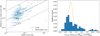 |
Fig. 5 Left panel: 2RXS vs. eFEDS count rates for the sources in common to both catalogues. The solid black line corresponds to the median count rate ratio of 5.8. The dashed lines correspond to a variability factor of 10 with respect to the median ratio (black solid line). Sources with variability factors >6 are marked with green or orange squares. Right panel: distribution of the variability factor. The orange line displays the standard normal distribution (unity scatter, zero mean). |
eFEDS – 2RXS sources with variability factors greater than 6.
6 Comparison with the XMM-ATLAS field
The eFEDS field overlaps with one of the wide-area and shallow surveys carried out by XMM-Newton: the XMM-ATLAS survey (Ranalli et al. 2015). The XMM observations were obtained in May 2013 and cover a total area of about 6 deg2. Comparing this data set with the eFEDS observations provides the opportunity of exploring the X-ray variability over a 6.5 yr timescale. This section reports X-ray sources that show evidence for significant variations in their X-ray flux between the eFEDS and the XMM-ATLAS epochs. The comparison is not limited to sources detected in both observations, but also uses upper limits when sources are detected by one telescope but not by the other.
A custom reduction of the XMM-ATLAS survey data was used based on the methods described by Georgakakis & Nandra (2011). The advantage of using a custom analysis rather than the publicly available XMM-ATLAS catalogue is the better control over the X-ray sensitivity, which is important for the calculation of upper limits. The relevant XMM-Newton observations (with identification numbers 0725290101, 0725300101, and 0725310101) were reduced using the XMM-Newton Science Analysis System (SAS) version 18. Sources were detected independently in three energy intervals, 0.5–2, 2–8, or 0.5– 8 keV with a Poisson false-detection threshold of <4 × 10⁻⁶. We detected 987 sources in the 0.5–2 keV band to the threshold above. The calculation of fluxes is based on aperture photometry using the Bayesian method described by Laird et al. (2009) and Georgakakis & Nandra (2011). The advantage of this approach is that it accounts for the Eddington bias in the determination of fluxes, which is expected to become important in the low-count regime of these X-ray imaging observations. When we assume that N is the total number of counts extracted within an aperture of radius R and В is the corresponding background level, the probability of a source with flux fx is given by the Poisson formula
 (5)
(5)
where π(fX) reflects the prior knowledge on the distribution of source fluxes, that is, the differential X-ray source number counts described by a double power law (e.g. Georgakakis et al. 2008). This term accounts for the Eddington bias. The quantity λ is the expected number of photons in the extraction cell for a source with flux fX,
 (6)
(6)
where ti is the exposure time, ECFi is the energy flux to photon flux conversion factor and depends on the spectral shape of the source. The summation in the equation above is for the three EPIC detectors (pn, MOS1, and MOS2). The calculation above assumes that the radius R of the extraction aperture corresponds to a fixed encircled energy fraction (EEF) of the XMM-Newton PSF. In our analysis the value of the EEF was set to 80%. Equation (5) can be numerically integrated (see Kraft et al. 1991) to determine the most likely value of fX and the corresponding uncertainties at a given confidence level. In the case of non-detections, the same equation can be integrated to determine upper limits. Fluxes for the XMM-ATLAS sources were estimated in the 0.5–2 keV spectral band assuming a power-law spectral model with Г = 1.4 that is absorbed by a Galactic column density of log NH/cm−2 = 20.3.
The main catalogue of the eFEDS field consists of sources detected in a single spectral band, 0.6–2.3 keV. This was chosen because the sensitivity of eROSITA peaks in this energy interval. Forced photometry in other spectral bands, including the 0.5–2 keV, is also available at the positions of the X-ray sources of the main eFEDS catalogue. Two independent approaches were adopted for the X-ray photometry. The first fits a model of the eROSITA PSF to the two-dimensional distribution of X-ray photons at a given position (ERMLDET task of eSASS). The second extracts counts within an aperture with a size that corresponds to a fixed EEF (APETOOL task of eSASS). Here we used the aperture photometry products (total counts, background level, and exposure time) to determine the source fluxes in the 0.5–2 keV band using the Bayesian method outlined above. The same spectral model as in the case of the XMM-ATLAS analysis was adopted. The aperture radius corresponds to the 60% EEF. In the remaining analysis, we consider a total of 985 eFEDS sources that lie within the XMM-ATLAS footprint and have a detection likelihood in the 0.6–2.3 keV band DET_LIKE > 10. This threshold was applied reduce the effect of spurious detections.
The first step was to match the eFEDS and XMM-ATLAS sources using a search radius of 15 arcsec. For the sky density of the XMM and ATLAS sources, this threshold corresponds to ≪ l spurious associations. Figure 6 compares the 0.5–2 keV fluxes of the 616 sources in common to the two surveys. The error bars correspond to the 68% confidence interval. The data points in this figure scatter around the one-to-one relation without evidence for strong systematic offsets. The scatter increases toward fainter fluxes because of the larger shot noise. This is further explored in the bottom panel of Fig. 6, which plots the histogram of the flux difference between eFEDS and XMM-ATLAS normalised to the flux errors added in quadrature. However, some sources show significant variations in flux between the two epochs. We attribute these differences to the intrinsic variability of accretion events and highlight the most extreme examples by selecting sources with flux variations of at least a factor of 6. These sources are highlighted in Fig. 6 and are listed in Table 4. Four of these seven variable sources are associated with spectroscopically confirmed AGN at z < 1.
The analysis above is based on the comparison of the X-ray fluxes of sources detected in both the XMM-ATLAS and eFEDS fields and will therefore miss variability events that reduce the flux of a source below the formal detection limit at either the XMM or the eROSITA epoch. Examples of these variable sources are identified in XMM-ATLAS detections without counterparts in the eFEDS survey and vice versa. The flux of a source at the detection epoch is compared with the 3σ upper limit on its flux estimated for the observation in which it lies below the detection threshold. This comparison can distinguish true variability events from non-detections because of either low effective exposure times (e.g. shallow observations or large off-axis angles) or high background levels. The estimation of upper limits uses aperture photometry and follows the methods described by Ruiz et al. (2022) based on Kraft et al. (1991). The probability density function of Eq. (5) is integrated with respect to fX to determine the corresponding cumulative distribution as a function of this parameter. The upper limit, UL, at an arbitrary confidence interval CL is then defined as the flux value at which the cumulative probability equals CL,
 (7)
(7)
where С is a normalisation constant. In calculating upper limits, we assumed a flat prior π(fX) in Eq. (5) and a confidence level CL = 99.87% that the true flux lies below the respective upper limit. This probability corresponds to the one-sided 3σ limit of a Gaussian distribution. First, we considered XMM-ATLAS sources without eFEDS counterparts within 30 arcsec. Using an aperture with radius of 60% EEF, we determined the eFEDS counts, background level, and exposure time at the positions of the XMM-ATLAS detections. Equations (6) and (7) were then used to determine the eROSITA epoch 3cr upper limits on the source fluxes. The comparison of the eROSITA upper limits and the XMM-ATLAS fluxes is shown in Fig. 7. Table 5 presents the selected sources with flux ratio between the eFEDS and XMM epochs >2. As a demonstration, Fig. 8 shows the XMM-ATLAS and eROSITA/eFEDS X-ray postage stamp images of one of the sources presented in Table 5.
Next, eFEDS X-ray sources that were not detected in the XMM-ATLAS observations were considered, defined as eROSITA sources without XMM-ATLAS counterparts within 30 arcsec. For this class of sources, a 3σ upper limit was estimated for their XMM-Newton fluxes in the 0.5–2 keV band. The upper-limit calculations is based on aperture photometry, as explained above. The radius of the extraction cell corresponds to the 80% EEF of the XMM-Newton PSF. The comparison of the eROSITA fluxes and XMM upper limits is shown in Fig. 9. Table 6 presents the sample of sources with flux ratios between the eFEDS and XMM epochs ≳2. Figure 10 shows the XMM-ATLAS and eROSITA/eFEDS X-ray postage stamp images of one of the sources presented in Table 6.
The left panel displays the 2RXS vs. eFEDS count rates for the sources in common to both catalogues. The solid black line corresponds to the median count rate ratio of 5.8. The dashed lines correspond to a variability factor of 10 from the median ratio. Sources with variability factors >6 are marked with green or orange squares. The right panel displays the distribution of the variability factor (with respect to the solid black line in the left panel).
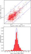 |
Fig. 6 Top panel: XMM-Atlas vs. eFEDS fluxes in the 0.5–2 keV band. The solid blue line shows the one-to-one relation. The dotted blue lines correspond to a flux ratio of 6. Sources with fluxes that differ by more than this factor in the two surveys are shown in blue. Bottom panel: distribution of the flux difference of X-ray sources between the XMM-ATLAS and eFEDS observations. The blue line shows a Gaussian distribution with zero mean and unity scatter. The histogram of the normalised flux difference has more power in the wings than in the normal distribution, which we attribute to variability. |
XMM-ATLAS and eFEDS source associations with flux ratio between the two surveys >6.
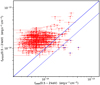 |
Fig. 7 XMM-ATLAS 0.5–2 keV flux vs. eFEDS flux upper limit (3σ–confidence) in the 0.5–2 keV band. Each data point in this plot corresponds to an XMM-ATLAS source detection without a counterpart in the eFEDS source catalogue. For these sources, the 3σ flux upper limits were estimated from the eFEDS observations and are plotted on the vertical axis. The dashed blue line indicates the one-to-one relation. The dotted blue line corresponds to a factor of two in flux relative to the one-to-one relation, i.e. sources with eFEDS 3σ flux upper limits that are twice fainter than the XMM-ATLAS source flux. Sources below this line are highlighted in blue. They were visually inspected to exclude spurious XMM-ATLAS sources and sources close to edge of the FOV. The resulting sample following the visual inspection is listed in Table 5. |
XMM-ATLAS source detections without counterparts in the eFEDS and flux ratio between the XMM flux and the eFEDS 3σ upper limit >2.
eFEDS source detections without counterparts in the XMM-ATLAS survey and flux ratio between the eFEDS flux and the XMM-ATLAS 3σ upper limit >2.
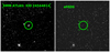 |
Fig. 8 X-ray postage stamp image of a source detected in the XMM-ATLAS survey without counterpart in the eFEDS and a ratio of the XMM 0.5–2 keV flux and the eFEDS 0.5–2.0 keV 3σ upper limit >2. The green circles mark the position of the source in the two observations and have a radius of 30 arcsec. |
7 Summary
We have studied the time variability of the eFEDS X-ray sources on short timescales within the eFEDS dataset and on longer timescales by comparison to the ROSAT all-sky and XMM-ATLAS surveys. About half of the variable objects are detected for the first time in X-rays with eROSITA. The number of sources for which significant soft-band variability was found within the eFEDS observation is relatively low (65 sources), and most of them are late-type stars of spectral type K and M (cf. Table 1). The eFEDS survey scanning strategy (where up to six consecutive data points with time bin sizes of 100 s are covered, followed by a time gap of about 3600 s, up to about 22000 s is very sensitive to stellar flaring events with decay times of a few thousand seconds. This is more efficient than the eROSITA all-sky survey and the ROSAT all-sky survey observations. Our fits to the eFEDS light curves for the most highly variable sources revealed some extreme stellar flare properties. We cross-matched the 2RXS catalogue with the eFEDS source catalogue and found that 12 sources show variability factors greater than six. We find six XMM-ATLAS detections with below the eFEDS 3σ upper limits. Nine sources have eFEDS source detections without a counterpart in the XMM-Atlas survey. Based on the variability studies in the eFEDS field, we expect about 20 000 variable sources after completion of the eROSITA all-sky survey outside the ecliptic pole regions.
The different time sampling of eFEDS and the eROSITA all-sky surveys will qualitatively affect their related variability information. The scan rate in the eROSITA all-sky survey is about seven times faster than in the eFEDS field scan (90 arc-sec s−1 compared to 13.15 arcsec s−1), and thus typical FOV passing times will be seven times shorter (40 s for central passage). The survey rate (progression in ecliptic longitude from one survey great circle to the next) is about 14arcmin/4h for the eFEDS region (about 4–5 passages over a source during one all-sky survey). However, the strength of the eROSITA all-sky survey observations will be the comparison between eight different epochs, providing the potential of analysing long-term variability over a four-year period.
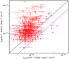 |
Fig. 9 eFEDS 0.5–2 keV flux vs. XMM-ATLAS flux upper-limit (3σ confldence) in the 0.5–2 keV. Each data point in this plot corresponds to an eFEDS source detection without a counterpart in the eFEDS source catalogue. For these sources, the 3σ flux upper limits are estimated from the XMM-ATLAS observations and plotted on the vertical axis. The solid blue line indicates the one-to-one relation. The dotted blue line corresponds to a factor of two in flux relative to the one-to-one relation, i.e. sources with XMM-ATLAS 3σ flux upper limits that are twice fainter than the XMM-ATLAS source flux. Sources below this line are highlighted in blue. Their properties are listed in Table 6. |
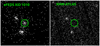 |
Fig. 10 eROSITA and XMM postage stamp images of an eFEDs X-ray source (see Table 6) without X-ray counterpart in the XMM-ATLAS survey. The green circles mark the position of the source in the two observations and have a radius of 30 arcsec. |
Acknowledgements
We thank the anonymous referee for their careful reading of the submitted manuscript, and for their very helpful comments and suggestions. M.K. acknowledges support by DFG grant KR 3338/4-1. This work is based on data from eROSITA, the soft X-ray instrument aboard SRG, a joint Russian-German science mission supported by the Russian Space Agency (Roskosmos), in the interests of the Russian Academy of Sciences represented by its Space Research Institute (IKI), and the Deutsches Zentrum für Luft- und Raumfahrt (DLR). The SRG spacecraft was built by Lavochkin Association (NPOL) and its subcontractors, and is operated by NPOL with support from the Max Planck Institute for Extraterrestrial Physics (MPE). The development and construction of the eROSITA X-ray instrument was led by MPE, with contributions from the Dr. Karl Remeis Observatory Bamberg & ECAP (FAU Erlangen-Nuernberg), the University of Hamburg Observatory, the Leibniz Institute for Astrophysics Potsdam (AIP), and the Institute for Astronomy and Astrophysics of the University of Tübingen, with the support of DLR and the Max Planck Society. The Argelander Institute for Astronomy of the University of Bonn and the Ludwig Maximilians Universität Munich also participated in the science preparation for eROSITA. The eROSITA data shown here were processed using the eSASS/NRTA software system developed by the German eROSITA consortium.
References
- Astropy Collaboration (Robitaille, T. P., et al.) 2013, A&A, 558, A33 [NASA ADS] [CrossRef] [EDP Sciences] [Google Scholar]
- Astropy Collaboration (Price-Whelan, A. M., et al.) 2018, AJ, 156, 123 [Google Scholar]
- Boller, T., Freyberg, M. J., Trümper, J., et al. 2016, A&A, 588, A103 [NASA ADS] [CrossRef] [EDP Sciences] [Google Scholar]
- Brunner, H., Liu, T., Lamer, G., et al. 2022, A&A, 661, A1 (eROSITA EDR SI) [NASA ADS] [CrossRef] [EDP Sciences] [Google Scholar]
- Buchner, J. 2014, Stat. Comput., 26, 1 [NASA ADS] [Google Scholar]
- Buchner, J. 2019, PASP, 131, 108005 [Google Scholar]
- Buchner, J. 2021, J. Open Source Softw., 6, 3001 [CrossRef] [Google Scholar]
- Buchner, J., Boller, T., Bogensberger, D., et al. 2022, A&A, 661, A18 (eROSITA EDR SI) [NASA ADS] [CrossRef] [EDP Sciences] [Google Scholar]
- Edelson, R. A., Krolik, J. H., & Pike, G. F. 1990, ApJ, 359, 86 [NASA ADS] [CrossRef] [Google Scholar]
- Edelson, R., Turner, T. J., Pounds, K., et al. 2002, ApJ, 568, 610 [CrossRef] [Google Scholar]
- Fuhrmeister, B., & Schmitt, J. H. M. M. 2003, A&A, 403, 247 [NASA ADS] [CrossRef] [EDP Sciences] [Google Scholar]
- Gehrels, N. 1986, ApJ, 303, 336 [Google Scholar]
- Georgakakis, A., & Nandra, K. 2011, MNRAS, 414, 992 [NASA ADS] [CrossRef] [Google Scholar]
- Georgakakis, A., Nandra, K., Laird, E. S., Aird, J., & Trichas, M. 2008, MNRAS, 388, 1205 [Google Scholar]
- Günther, M. N., Zhan, Z., Seager, S., et al. 2020, AJ, 159, 60 [Google Scholar]
- Kerr, M. 2019, ApJ, 885, 92 [NASA ADS] [CrossRef] [Google Scholar]
- Kraft, R. P., Burrows, D. N., & Nousek, J. A. 1991, ApJ, 374, 344 [Google Scholar]
- Laird, E. S., Nandra, K., Georgakakis, A., et al. 2009, ApJS, 180, 102 [NASA ADS] [CrossRef] [Google Scholar]
- Liu, T., Buchner, J., Nandra, K., et al. 2022, A&A, 661, A5 (eROSITA EDR SI) [NASA ADS] [CrossRef] [EDP Sciences] [Google Scholar]
- Magaudda, E., Stelzer, B., Raetz, St., et al. 2022, A&A, 661, A29 (eROSITA EDR SI) [NASA ADS] [CrossRef] [EDP Sciences] [Google Scholar]
- Nandra, K., George, I. M., Mushotzky, R. F., Turner, T. J., & Yaqoob, T. 1997, ApJ, 476, 70 [Google Scholar]
- Pecaut, M. J., & Mamajek, E. E. 2013, ApJS, 208, 9 [Google Scholar]
- Predehl, P., Andritschke, R., Arefiev, V., et al. 2021, A&A, 647, A1 [EDP Sciences] [Google Scholar]
- Ranalli, P., Georgantopoulos, I., Corral, A., et al. 2015, A&A, 577, A121 [NASA ADS] [CrossRef] [EDP Sciences] [Google Scholar]
- Ruiz, A., Georgakakis, A., Gerakakis, S., et al. 2022, MNRAS, 511, 4265 [NASA ADS] [CrossRef] [Google Scholar]
- Salvato, M., Wolf, J., Dwelly, T., et al. 2022, A&A, 661, A3 [NASA ADS] [CrossRef] [EDP Sciences] [Google Scholar]
- Scargle, J. D., Norris, J. P., Jackson, B., & Chiang, J. 2013, ApJ, 764, 167 [Google Scholar]
- Schmitt, J. H. M. M., Ioannidis, P., Robrade, J., Czesla, S., & Schneider, P. C. 2019, A&A, 628, A79 [NASA ADS] [CrossRef] [EDP Sciences] [Google Scholar]
- Schmitt, J. H. M. M., Ioannidis, P., Robrade, J., et al. 2021, A&A, 652, A135 (eROSITA EDR SI) [NASA ADS] [CrossRef] [EDP Sciences] [Google Scholar]
- Vaughan, S., Edelson, R., Warwick, R. S., & Uttley, P. 2003, MNRAS, 345, 1271 [Google Scholar]
All Tables
Most variable eFEDS sources in the energy band (0.2–2.3) keV ordered in descending maximum amplitude values.
XMM-ATLAS and eFEDS source associations with flux ratio between the two surveys >6.
XMM-ATLAS source detections without counterparts in the eFEDS and flux ratio between the XMM flux and the eFEDS 3σ upper limit >2.
eFEDS source detections without counterparts in the XMM-ATLAS survey and flux ratio between the eFEDS flux and the XMM-ATLAS 3σ upper limit >2.
All Figures
|
Fig. 1 Sample distribution in mean count rate and ampl_max. For each test, the sources considered significantly variable are marked. While most of these markers are limited to the upper left corner, the blue crosses extend to the bottom left corner of the plot. This reflects the sensitivity of bexvar in the low count-rate regime. |
| In the text | |
|
Fig. 2 Light curves (top two panels) and cumulative count plots (lower two panels) for two eFEDS sources (source IDs 2 and 837). The grey shadowed areas in the cumulative plots indicate count rate deviations of 1, 2, and 3σ with respect to a constant count rate per cumulative time bin. |
| In the text | |
|
Fig. 3 Light curves for the 12 most variable eFEDS sources. The bin size is 100 s and the energy band is band 1. The objects are ordered from top left to right bottom in descending maximum amplitude σ values. For the normalized excess variance and the maximum amplitude variability the values in units of σ are indicated along the top of each panel. The variability flags (T for true and F for false) are also listed for the Bayesian excess variance (bexvar), and the Bayesian block method (nblocks). |
| In the text | |
|
Fig. 4 Fits to stellar flares for objects in Table 1 with source identifications 2, 5, 6, 77, 95, and 413 (from top left to bottom right). |
| In the text | |
|
Fig. 5 Left panel: 2RXS vs. eFEDS count rates for the sources in common to both catalogues. The solid black line corresponds to the median count rate ratio of 5.8. The dashed lines correspond to a variability factor of 10 with respect to the median ratio (black solid line). Sources with variability factors >6 are marked with green or orange squares. Right panel: distribution of the variability factor. The orange line displays the standard normal distribution (unity scatter, zero mean). |
| In the text | |
|
Fig. 6 Top panel: XMM-Atlas vs. eFEDS fluxes in the 0.5–2 keV band. The solid blue line shows the one-to-one relation. The dotted blue lines correspond to a flux ratio of 6. Sources with fluxes that differ by more than this factor in the two surveys are shown in blue. Bottom panel: distribution of the flux difference of X-ray sources between the XMM-ATLAS and eFEDS observations. The blue line shows a Gaussian distribution with zero mean and unity scatter. The histogram of the normalised flux difference has more power in the wings than in the normal distribution, which we attribute to variability. |
| In the text | |
|
Fig. 7 XMM-ATLAS 0.5–2 keV flux vs. eFEDS flux upper limit (3σ–confidence) in the 0.5–2 keV band. Each data point in this plot corresponds to an XMM-ATLAS source detection without a counterpart in the eFEDS source catalogue. For these sources, the 3σ flux upper limits were estimated from the eFEDS observations and are plotted on the vertical axis. The dashed blue line indicates the one-to-one relation. The dotted blue line corresponds to a factor of two in flux relative to the one-to-one relation, i.e. sources with eFEDS 3σ flux upper limits that are twice fainter than the XMM-ATLAS source flux. Sources below this line are highlighted in blue. They were visually inspected to exclude spurious XMM-ATLAS sources and sources close to edge of the FOV. The resulting sample following the visual inspection is listed in Table 5. |
| In the text | |
|
Fig. 8 X-ray postage stamp image of a source detected in the XMM-ATLAS survey without counterpart in the eFEDS and a ratio of the XMM 0.5–2 keV flux and the eFEDS 0.5–2.0 keV 3σ upper limit >2. The green circles mark the position of the source in the two observations and have a radius of 30 arcsec. |
| In the text | |
|
Fig. 9 eFEDS 0.5–2 keV flux vs. XMM-ATLAS flux upper-limit (3σ confldence) in the 0.5–2 keV. Each data point in this plot corresponds to an eFEDS source detection without a counterpart in the eFEDS source catalogue. For these sources, the 3σ flux upper limits are estimated from the XMM-ATLAS observations and plotted on the vertical axis. The solid blue line indicates the one-to-one relation. The dotted blue line corresponds to a factor of two in flux relative to the one-to-one relation, i.e. sources with XMM-ATLAS 3σ flux upper limits that are twice fainter than the XMM-ATLAS source flux. Sources below this line are highlighted in blue. Their properties are listed in Table 6. |
| In the text | |
|
Fig. 10 eROSITA and XMM postage stamp images of an eFEDs X-ray source (see Table 6) without X-ray counterpart in the XMM-ATLAS survey. The green circles mark the position of the source in the two observations and have a radius of 30 arcsec. |
| In the text | |
Current usage metrics show cumulative count of Article Views (full-text article views including HTML views, PDF and ePub downloads, according to the available data) and Abstracts Views on Vision4Press platform.
Data correspond to usage on the plateform after 2015. The current usage metrics is available 48-96 hours after online publication and is updated daily on week days.
Initial download of the metrics may take a while.