| Issue |
A&A
Volume 660, April 2022
|
|
|---|---|---|
| Article Number | A123 | |
| Number of page(s) | 17 | |
| Section | Planets and planetary systems | |
| DOI | https://doi.org/10.1051/0004-6361/202142135 | |
| Published online | 29 April 2022 | |
Physically-motivated basis functions for temperature maps of exoplanets
1
Center for Space and Habitability, University of Bern,
Gesellschaftsstrasse 6,
3012
Bern, Switzerland
e-mail: This email address is being protected from spambots. You need JavaScript enabled to view it.
2
Department of Physics, Astronomy & Astrophysics Group, University of Warwick,
Coventry
CV4 7AL, UK
3
Ludwig Maximilian University, University Observatory Munich,
Scheinerstrasse 1,
Munich
81679, Germany
4
Institut de recherche sur les exoplanètes, Département de physique, Université de Montréal,
2900 boul. Édouard-Montpetit,
Montreal, QC
H3T 1J4, Canada
5
Lund Observatory, Department of Astronomy and Theoretical Physics, Lunds Universitet,
Solvegatan 9,
222 24
Lund, Sweden
Received:
2
September
2021
Accepted:
22
October
2021
Abstract
Thermal phase curves of exoplanet atmospheres have revealed temperature maps as a function of planetary longitude, often by sinusoidal decomposition of the phase curve. We construct a framework for describing two-dimensional temperature maps of exoplanets with mathematical basis functions derived for a fluid layer on a rotating, heated sphere with drag/friction, which are generalisations of spherical harmonics. These basis functions naturally produce physically-motivated temperature maps for exoplanets with few free parameters. We investigate best practices for applying this framework to temperature maps of hot Jupiters by splitting the problem into two parts: (1) we constrain the temperature map as a function of latitude by tuning the basis functions to reproduce general circulation model outputs, since disk-integrated phase curve observations do not constrain this dimension; and (2) we infer the temperature maps of real hot Jupiters using original reductions of several Spitzer phase curves, which directly constrain the temperature variations with longitude. The resulting phase curves can be described with only three free parameters per bandpass – an efficiency improvement over the usual five or so used to describe sinusoidal decompositions of phase curves. Upon obtaining the hemispherically averaged day side and night side temperatures, the standard approach would be to use zero-dimensional box models to infer the Bond albedo and redistribution efficiency. We elucidate the limitation of these box models by demonstrating that negative Bond albedos may be obtained due to a choice of boundary condition on the night side temperature. We propose generalized definitions for the Bond albedo and heat redistribution efficiency for use with two-dimensional (2D) temperature maps. Open-source software called kelp is provided to efficiently compute the 2D temperature maps, phase curves, albedos and redistribution efficiencies.
Key words: radio continuum: planetary systems / planets and satellites: atmospheres / planets and satellites: gaseous planets / techniques: photometric / methods: analytical / methods: observational
Hans Sigrist Foundation PhD Fellow.
© ESO 2022
1 Introduction
We can directly observe the disk-integrated light from exoplanet atmospheres by measuring their phase curves, or the apparent brightness of the star-planet system as a function of orbital phase (see review by Parmentier & Crossfield 2018). Phase curve observations of close-in, hot exoplanets can reveal hints of atmospheric heat redistribution (Knutson et al. 2007), typically observed as a hot spot offset in longitude from the synchronously rotating sub-stellar point (Cowan & Fujii 2018; Madhusudhan 2019). By searching for variations in the phase curve with time, one can search for signatures of non-steady-state dynamics in exoplanet atmospheres (e.g. Heng & Showman 2015).
One technique for fitting the phase curves of hot exoplan-ets was presented by Cowan & Agol (2008), which essentially applies Fourier’s theorem to phase curves. It demonstrates that a mixture of a few sinusoidal components can fit most phase curves with a relatively small number of free parameters. Cowan & Agol (2008) study the information loss as one takes disk-integrated observations of exoplanet atmospheres, showing that the light curve can only sufficiently constrain roughly five free parameters. Knutson et al. (2007); Hu et al. (2015) fit the more demanding light curves of HD 189733 b and Kepler-7 b with a “beach-ball” model, with longitudinal segments at different temperatures.
Several works have used spherical harmonics to describe the maps of hot exoplanets. For example, Cowan et al. (2013) derived phase curves for spherical harmonic basis maps, Rauscher et al. (2018) fit for the temperature map of HD 189733 b with a spherical harmonic expansion and a dimensionality reduction technique, and Luger et al. (2019) derive closed-form solutions for phase curves and occultations of planetary flux maps represented with spherical harmonics. One strength of these approaches is that any planetary temperature map can be represented at sufficiently large degrees, and one possible weakness is that the flexible fits may correspond to implausible climate scenarios.
Matsuno (1966) and Longuet-Higgins (1968) previously showed that a reduced set of two-dimensional fluid equations (the so-called “shallow water system” or Laplace’s tidal equations) on a rotating sphere may be reduced to the quantum harmonic oscillator equation. The shallow water framework has been applied to the atmospheres of neutron stars (Heng & Spitkovsky 2009), the solar tachocline (Gilman 2000), the atmosphere of the Earth (Gill 1980), the top layer of the core of the Earth (Braginsky 1998) and the behaviour of submerged islands in the ocean of the Earth (Longuet-Higgins 1967). In the absence of rotation, the solutions to the shallow water framework are the familiar spherical harmonics. With rotation, the solutions are the so-called “parabolic cylinder functions”, which are combinations of exponential functions and Hermite polynomials. Heng & Workman (2014) further showed that when stellar heating (forcing) and drag/friction (both hydrodynamic and mag-netohydrodynamic) are added to the system, one still obtains the parabolic cylinder functions in certain limits. For brevity, we will refer to these functions as the hmℓ generalised spherical harmonic basis and use them to describe exoplanet photospheric temperature maps.
There are several advantages to using the hmℓ basis functions to describe an exoplanet’s 2D temperature map: (1) the input arguments to the special functions, α and ωdrag, are physically-meaningful parameters which represent properties of the atmosphere; (2) it is equally straightforward to fit the 2D basis function description of the temperature map to general circulation model (GCM) simulations and to observations of real exoplanets, allowing theory and observation to be compared in the same mathematical language; (3) even when limited to only a few free parameters, the hmℓ basis can reproduce a diverse range of phase curve phenomena including offset hots pots and chevron-shaped hot regions. We will show in this work that some of the physically-meaningful parameters can be constrained using fits of the hmℓ basis to GCMs, which reduces the total number of free parameters in fits to phase curve observations.
In Sect. 2, we outline the hmℓ basis functions used to compute the temperature map and the phase curves from the temperature map. In Sect. 3, we develop formalism for measuring Bond albedos and redistribution efficiencies from 2D temperature maps. In Sect. 4, we outline a technique for constraining the latitudinal temperature distributions of hot exoplanets by fitting the hmℓ basis functions to the 2D temperature maps produced by GCMs. In Sect. 5, we fit phase curve observations from Spitzer using priors extracted from the fits to the GCM temperature maps, and compare results obtained from fitting the Spitzer phase curves and the GCMs. We discuss the results in Sect. 6 and conclude in Sect. 7.
2 Phase curve model
Mathematically, hmℓ is the perturbation to the height of the fluid in the so-called “shallow water system”, which is a proxy for the temperature perturbation (Cho et al. 2008). Therefore, we define a 2D temperature map as a function of latitude and longitude T (θ,ϕ):
 (1)
(1)
The prefactor  on the right hand side acts as a constant scaling term for the mean temperature field, on which the hmℓ terms are a perturbation. A plausible initial guess for the value of this prefactor is
  for stellar effective temperature T⋆, and normalized semimajor axis
  is the Bond albedo and ƒ′ may be interpreted either geometrically (see Sect. 3.1) or as a greenhouse factor. We mark the ƒ′ and
  variables with primes here to denote that these two terms will be redefined in Sect. 3, and thus we do not report the values of the primed variables in this work. We note that the two terms in the factor
  are perfectly degenerate.
For efficient sampling of all plausible temperature maps given the degenerate parameterization of the two-parameter term  in Eq. (1), we take the following conventions in generating temperature maps: (1) we set
  in Eq. (1) to zero always, and (2) we allow ƒ′ to vary uniformly from zero to unity, which extends beyond the range normally given to this parameter in the literature. The net effects of these choices are that (1) the two free parameters ƒ′ and
  are sampled as a single free parameter which describes
  , and (2) the parameters provided to the sampler
 ![Mathematical equation: $(f' \in [0 - 1],A_B^' = 0)$](/articles/aa/full_html/2022/04/aa42135-21/aa42135-21-eq11.png) need not be tracked during sampling. Instead, we infer the Bond albedo and the heat redistribution efficiency for a given temperature map by computing the temperature map with the parameter
need not be tracked during sampling. Instead, we infer the Bond albedo and the heat redistribution efficiency for a given temperature map by computing the temperature map with the parameter  , and then integrate outgoing flux from the planetary atmosphere to compute the Bond albedo and redistribution efficiency, as outlined in the Sect. 3.4.
The hml (α, ωdrag) terms are defined by Eq. (258) of Heng & Workman (2014),
![Mathematical equation: $\matrix{ {{h_{m\ell }} = {{{C_{m\ell }}} \over {\omega _{{\rm{drag}}}^2{\alpha ^4} + {m^2}}}{e^{ - {{\tilde \mu }^2}/2}}[\mu m{H_\ell }\cos (m\phi )} \hfill \cr {\quad \quad + \alpha {\omega _{{\rm{drag}}}}(2\ell {H_{\ell - 1}} - \tilde \mu {H_\ell })\sin (m\phi )],} \hfill \cr } $](/articles/aa/full_html/2022/04/aa42135-21/aa42135-21-eq13.png) (2)
(2)
where α is a dimensionless fluid number that is constructed from the Rossby, Reynolds and Prandtl numbers. ωdrag is the dimensionless drag frequency (normalised by twice the angular velocity of rotation),  are the physicist’s Hermite polynomials:

The hmℓ basis is derived without any special reference point in longitude. As a result, the hottest point on the atmosphere need not be the sub-stellar point. We parameterize shifts in the prime meridian of the hmℓ basis from the sub-stellar point using a simple phase offset parameter, Δϕ, which describes a rotation of the coordinate system about the pole. It is important to note that the phase offset parameter Δφ is not equivalent to the traditional “hotspot offset” parameter often used in the literature, which measures the difference in longitude between the hottest longitude and the sub-stellar longitude. The phase offset Δϕ will vary with ωdrag, though in practice, drag values approaching and above of ωdrag ≳ 3 correspond to maps where the hottest point on the map is practically indistinguishable from the sub stellar point. In the remainder of this paper, we will report the phase offset Δϕ parameter with the implicit caveat that the distinction between phase offset and hotspot offset is negligible for the large drag frequencies discussed here.
For a phase curve fit with ℓmax = 1, for example, the free parameters in the fit could include {C11, α, ωdrag, ƒ′, Δϕ}. In practice however, α and ωdrag control the latitudinal concentration of heat in the planet’s atmosphere, so these two parameters are unconstrained by the phase curve alone. In Sect. 4, we will determine reasonable values for α and ωdrag based on fits with the hmℓ basis to the 2D temperature maps produced by GCMs. These constraints can act as physically-motivated priors in the infrared phase curve fits which follow in Sect. 5.
The generalised spherical harmonic hmℓ basis defines an “alphabet” with only a few free parameters which we can use to succinctly describe exoplanet temperature fields, shown in Fig. 1. Each panel represents an individual generalized spherical harmonic expansion term, and we reconstruct temperature maps of exoplanets by evaluating linear combinations of these basis maps.
We have fully defined the temperature map of the planet with the parameters above, and now we must construct the Planck function ℬλ(T(θ, ϕ)), integrate ℬλ within the bandpass of observations, and then disk-integrate to construct a thermal phase curve. We integrate the ratio of flux from the planet and the host star (Cowan & Agol 2011a):
 (3)
(3)
where the intensity I is given by
 (4)
(4)
for a filter response function ℱλ. The above relation neglects any reflected light. We assume the spectrum of each host star is accurately described by PHOENIX model spectra with the nearest effective temperature and surface gravity (Husser et al. 2013).
We have developed an efficient Python package for computing this triple integral for time series phase curve observations, written with Cython, theano and JAX for maximum speed and readability, called kelp, which is publicly available1.
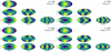 |
Fig. 1 Four montages of the first several terms in the generalized spherical harmonic expansion of the temperature map in the hmℓ basis. Each montage corresponds to a different combination of α and ωdrag, labeled in the upper right of each quadrant. Each map shows the temperature perturbation (purple to yellow is cold to hot) as a function of latitude and longitude (shown in Moll weide projections such that the sub stellar longitude is in the center of the plot). The m = 0 terms are always zero. The even-ℓ terms are asymmetric about the equator and therefore do not represent typical GCM results in equilibrium, so we keep all even-ℓ power coefficients fixed to zero in the subsequent fits (this approach assumes edge-on orbits, for exceptions see Cowan et al. 2017). In the upper two quadrants, when ωdrag is set to a smaller value, the chevron shape becomes more pronounced. In the two quadrants on the right, when the α is set to a larger value, the concentration of heat near the equator is more pronounced. |
3 From 0D to 2D: Bond Albedos and Redistribution Efficiencies
3.1 Background
Zero-dimensional (0D) “box models” are used ubiquitously in exoplanet science. As a prime example, the “equilibrium temperature” of an exoplanet is standard fare in publications (e.g. Seager 2010). It originates from considering the stellar irradiation received by, and subsequently re-radiated χπ steradians of, a spherical exoplanet. The stellar luminosity is  with R⋆ being the stellar radius and σSB the Stefan-Boltzmann constant. The star is approximated as a spherical black body with a uniform photospheric temperature T⋆. The stellar flux fills a celestial sphere with a surface area of 4πa2, where a is the distance between the star and exoplanet. The exoplanet presents a cross section of πR2 for intercepting this stellar flux, but absorbs only a fraction 1 – AB of it with AB being its Bond albedo. Therefore, the box model of luminosity received is
 (5)
(5)
Assuming the exoplanet to radiate like a black body, the box model of luminosity re-radiated by the exoplanet is
 (6)
(6)
where T is a characteristic temperature associated with the exoplanet. If we assume that its flux is re-radiated over χπ = 4π steradians, then one recovers the standard expression for the equilibrium temperature (e.g., Seager 2010),
 (7)
(7)
where  is the irradiation temperature. The equilibrium temperature is often quoted assuming AB = 0 (e.g., López-Morales & Seager 2007).
More generally, one may write ƒ = 1/χ as a redistribution factor and derive an expression for the he mispherically-averaged day side temperature of the exoplanet,
 (8)
(8)
where we define2 T0 ≡ Tirr(1 − AB)1/4. By analogy, one may write the he mispherically- averaged night side temperature as Tn = T0g1/4. By assuming a linear relationship between ƒ and g and applying the boundary conditions that ƒ = g = 1/4 for full heat redistribution and ƒ = 2/3 and g = 0 for no redistribution, one obtains
 (9)
(9)
One may also rewrite the preceding expressions in terms of a redistribution efficiency ε = 8/5 − 12 ƒ/5 that is bounded between 0 and 1, which yields Eqs. (4) and (5) of Cowan & Agol (2011b).
The day side and night side brightness temperatures of an exo-planet may be directly inferred from data. If one observes the secondary eclipse of an exoplanet purely in thermal emission, then the day side brightness temperature may be extracted in a model-independent way (Seager 2010). Extracting the night side brightness temperature requires a thermal phase curve to be measured as it is the difference in flux between the top of the transit and the bottom of the secondary eclipse (Schwartz et al. 2017). For example, the night side brightness temperature of 55 Cancri e was measured using a Spitzer phase curve (Demory et al. 2016a). It is worth noting that, in extracting the temperature map, Eq. (4) already accounts for thermal emission within a Spitzer bandpass. For a black body, the temperature and brightness temperature are equal.
Equations (8) and (9) may be inverted to solve for the Bond albedo and redistribution factor/efficiency, if the day side and night side (brightness) temperatures are known empirically. However, it is possible to obtain negative Bond albedos by using Eqs. (8) and (9). This artefact arises from approximating a two-dimensional (2D) situation with a 0D box model and is tied to the choice of boundary condition made for g, which we will next demonstrate. It affects the inference of AB and ƒ or ε from all thermal phase curves of exoplanets.
3.2 General Box Models
Starting again from Tn = T0g1/4, we apply more general boundary conditions on g:
 (10)
(10)
This yields a general expression for g in terms of ƒ and ƒ0,
 (11)
(11)
Similarly, more general boundary conditions on ε are:
 (12)
(12)
which yields
 (13)
(13)
The general expression for the day side temperature is
 (14)
(14)
The general expression for the night side temperature is
 (15)
(15)
In the limit of ƒ0 = 2/3 (Hansen 2008), we recover Eq. (4) of Cowan & Agol (2011b) for the dayside temperature.
If we define the contrast between the night side and day side hemispheric temperatures as C = Tn/Td, then the redistribution factor may be expressed as
 (16)
(16)
3.3 Why Box Models May Produce Negative Bond Albedos
One may rewrite the expression for the day side temperature in Eq. (14) to obtain an expression for the Bond albedo,
 (17)
(17)
If we demand that AB < 0, then we obtain the following inequality,
 (18)
(18)
In the high-temperature limit, we expect C ≈ 0 and ƒ ≈ ƒ0. Therefore, negative Bond albedos are obtained when 
It only remains to derive the value of ƒ0. The standard value of ƒ0 = 2/3 is obtained from adding an irradiation term to the expression for the intensity associated with Milne’s solution (Hansen 2008). Section 2.2 of Cowan & Agol (2011b) discusses how other choices may be made. In the context of our box models, we may write
 (19)
(19)
where the integration from ϕ = −π/2 to π/2 occurs only over the dayside hemisphere. If the day side flux of the exoplanet is F = σSBT4 and T is assumed to be constant, then we recover L'′= 2πR2σSB T4, χ = 2 and ƒ0 = 1/2. If we account approximately for anisotropic emission over the day side hemisphere (caused by anisotropic stellar irradiation; Hansen 2008) by writing F = σSBT4 sin θ, then we obtain ƒ0 = 2/π ≈ 0.64. This assumes that the radiative times cale is much shorter than the dynamical timescale (López-Morales & Seager 2007).
Table 8 of Wong et al. (2021) lists the dayside and irradiation temperatures of several hot Jupiters obtained from analysing Spitzer data. Specifically, it allows us to estimate Td/Tirr values of 0.96 ± 0.04 for HAT-P-7b, 0.94 ± 0.05 for KELT-1b, 0.92 ± 0.02 for WASP-18b and 0.83 ± 0.02 for WASP-33b.
Figure 2 demonstrates that these estimates of Td/Tirr satisfy the condition for negative Bond albedos stated in Eq. (18). Unsurprisingly, Table 8 of Wong et al. (2021) lists a negative Bond albedo for HAT-P-7b.
Generally, if the empirically-obtained value of Td/Tirr exceeds about 0.9 (with this exact threshold depending on the assumed value of f0, then the use of Eqs. (8) and (9) results in a negative value for the Bond albedo. This artifact originates from the global non-conservation of energy.
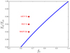 |
Fig. 2 Lower limit on Td/Tirr (curve) for producing negative Bond albedos. For comparison, empirically obtained values of Td/Tirr from Wong et al. (2021) are shown; the uncertainties on these values (not shown for plot clarity) are between 2% and 5%. |
3.4 General Expression for Bond Albedo
We propose more general expressions for extracting AB and ε directly from a two-dimensional temperature map, which have been previously proposed in Keating et al. (2019). Generally, the expression for L in Eq. (5) holds regardless of one’s assumption on f0. However, the expression for L′in Eq. (6) needs to be generalised for application to infrared phase curves,
 (20)
(20)
A general expression for inference of the Bond albedo is
 (21)
(21)
The two-dimensional flux distribution F(θ, ϕ) may be inferred from an infrared phase curve, where the temperature T(θ, ϕ) is not assumed to be constant.
The redistribution efficiency is simply the ratio of the night-side to day side fluxes,
 (22)
(22)
3.5 Limitations of Two-Dimensional Models
While more general than 0D box models, the 2D temperature-map approach has the following limitations:
The atmospheric temperature generally varies in all three dimensions, implying that thermal phase curves measured at different wavelengths sample radial/vertical variations in temperature (Stevenson et al. 2014). In other words, a thermal phase curve at a specific wavelength probes a 2D surface; at other wavelengths, other surfaces are probed. These surfaces are generally not isobaric;
The spectral energy distribution of the exoplanet atmosphere may deviate strongly from a blackbody, especially far away from the black body peak where the intensity is proportional to λ−4 (Rayleigh-Jeans law). This implies that the brightness temperature is not the true local temperature.
In the limit of sparse data, it is plausible to combine the analysis of infrared phase curves, measured in two different Spitzer channels, to infer a 2D temperature map. In the era of the James Webb Space Telescope (JWST), the need for a three-dimensional approach will be urgently needed as it will affect the inference of Bond albedo values from JWST phase curves.
4 2D Temperature maps from GCMs
The incentive is strong to infer 2D temperature maps for exoplanets, despite the lack of constraints from phase curve observations. Planets such as KELT-9 b have dayside atmospheres as hot as a K star and night side temperatures as hot as an M star, and the distribution of temperature with latitude may be similarly extreme, spanning ~ 15OO K from pole to equator (see below). These tremendous temperature variations suggest that different chemistry may be important within the same planetary hemisphere. For example, this has important implications in translating what we learn from the phase curve into expectations for observations at the planet’s terminator, which is probed during transmission spectroscopy.
The disk-integration that occurs when constructing a phase curve in Eq. (3) effectively discards information about the distribution of temperatures with latitude. In some cases this information can be recovered for the day sides of exoplanets on slightly inclined orbits during secondary eclipse (see, e.g.: Majeau et al. 2012; de Wit et al. 2012). In general, however, the distribution of temperatures with latitude is not constrained by the phase curve.
In this section, we explore whether we can use three-dimensional GCMs to inform inferred temperature maps of real hot Jupiters from phase curve observations. We introduce a set of GCMs in the next subsection, then outline a procedure for fitting them in the following subsection. Finally, we summarize the results in the limit of a planet with very high irradiation.
4.1 GCM Simulations
Given that phase curves of exoplanets do not constrain the latitudinal distribution of heat in an exoplanet atmosphere, we will “observe” some ubiquitous trends in model atmospheres which set the expectations for the latitude distribution of heat in real exoplanet atmospheres. Perna et al. (2012) studied heat redistribution and energy dissipation in hot Jupiter atmospheres using three-dimensional circulation models with dual-band or “double grey” radiative transfer. The authors used the GCMs to infer the effects of temperature inversions and stellar irradiation on hotspot offsets from the substellar point, among other quantities. We summarize their grid of 16 GCMs in Table 1. The greenhouse parameter γ is the ratio of the mean infrared to optical/visible opacity and controls whether a temperature inversion is present (Guillot 2010); γ = 0.5 and 2 correspond to temperature-pressure profiles without and with inversions, respectively.
Initial and equilibrium temperatures of the GCM runs of Perna et al. (2012).
4.2 Fits to The GCM Temperature Maps
4.2.1 Phase Offset
The temperature map formulation by Heng & Workman (2014) is constructed without any special definitions for an origin in longitude, ϕ. As a result, the temperature maps need a constant offset of π/2 to behave correctly in the limit of ωdrag ≫ 1, which ensures that the sub stellar point is also the hottest point on the map.
Similarly, we introduce an arbitrary phase offset as a fitting parameter, Δϕ, which allows the temperature map to be rotated with respect to the substellar point. While the hmℓ basis could in principle fit any temperature map at sufficiently large spherical harmonic degree, maps with significant hotspot offsets would require ℓmax ≫ 1 in order to approximate the offset temperature distribution, incurring many free Cmℓ parameters and making the inference intractable. Therefore, we introduce a single arbitrary rotation offset angle Δϕ to the fits of the temperature maps to concisely describe hotspot offsets at small ℓmax.
4.2.2 Empirical limits on ℓmax
As noted in the previous section, introducing the coordinate system offset angle Δϕ of the temperature map fits allows us to reproduce the GCM temperature maps with small ℓmax. Choosing ℓmax = 1 requires five free parameters: {ƒ, C11,α, ωdrag, Δϕ}. The ℓ = 2 maps are not important for fitting mean phase curves of exoplanets as they are not symmetric across the planetary equator, and therefore should not have significant power for an atmosphere near equilibrium (see Fig. 1). ℓmax = 3 has seven parameters, and so on. We first fit the 2D GCM temperature maps with the hmℓ basis using ℓmax = 3, and find that the three Cml terms for ℓ = 3 are constrained to be very small compared to the power in C11. We then inspect the quality of the fits for ℓmax = 1 and ℓmax = 3, and find that the ℓmax = 1 maps are indeed strikingly similar to the ℓmax = 3 maps, and thus we reason that ℓmax = 1 is likely sufficient to approximate temperature maps for phase curve analyses, requiring up to five free parameters.
We note that previous studies have suggested that about five free parameters can be constrained by fits to a 1D phase curve (Cowan & Agol 2011a; Hu et al. 2015). It is encouraging that we arrive at a similar conclusion about the information content of phase curves as studies that take very different approaches to constructing phase curves, but as we will discuss in the next subsection, if we narrow our focus to the hottest exoplanets we can collapse the parameter space further.
4.2.3 Trends Towards High Equilibrium Temperature
Next, we look for trends with irradiation in the physically meaningful fitting parameters with which we can constrain the 2D temperature maps of real exoplanets. We fit the 2D temperature maps of the Perna et al. (2012) GCMs for the parameters which control the 2D temperature map in the hmℓ basis with ℓmax = 1, {ƒ, Cmℓ, α, ωdrag, Δϕ}, using Markov chain Monte Carlo (Foreman-Mackey et al. 2013). The GCM temperature fields and the maximum-likelihood hmℓ maps are shown in Fig. 3. Comparison between the GCM results and the maximum-likelihood hmℓ reconstructions confirms that the major features of the map are reproduced by the hmℓ model at small ℓmax, and more subtle features are reproduced at large ℓmax. When α and ωdrag are allowed to vary, the concentration of heat near the equator is easily reproduced by the hmℓ basis.
Remarkably, the four hottest temperature maps in Fig. 3 can all be fit with similar α and ωdrag parameters, α = 0.6 and ωdrag = 4.5. This is demonstrated by the posterior distributions for α and ωdrag for each of the four hottest GCM maps in Fig. 4. In other words, the latitudinal temperature distribution across maps with varying equilibrium temperature is quite similar when phrased in terms of the hmℓ “alphabet”. The chevron shapes that are produced by this combination of α and ωdrag will be familiar to many GCM practitioners – it is a shape reproduced by many GCMs and has an elucidated theoretical basis (e.g.: Showman & Polvani 2011; Tsai et al. 2014).
At ℓmax = 3 we are unable to reproduce some of the subtle features of the map, such as the equatorial jet that is noticeable in the night side atmosphere, or the “point” that forms at the leading edge of the day side atmosphere. These features could be reproduced by going to higher ℓmax, but since we are focused here on jointly inferring properties from GCMs and phase curves, we assume that such fine features will remain undetectable with phase curve photometry, and neglect these small features. In the bottom row of Fig. 3, we show a linear hmℓ solution to the GCM temperature maps with ℓmax = 50, which better reproduces the precise shape of the dayside hotspot but not the jet, for example.
To summarize, our experiments fitting the hmℓ maps to the GCMs have shown that: (1) we must introduce a phase offset that was not accounted for in the original definition of the hmℓ basis; (2) ℓmax = 1 or 3 is likely sufficient to capture the global-scale temperature inhomogeneities that are routinely in agreement between different GCMs and likely to be constrained by the phase curves; (3) the hottest maps all demand a common combination of α = 0.6 and ωdrag = 4.5, collapsing our parameter space from five to three free parameters.
5 Spitzer Observations
Next, we apply the hmℓ basis functions in the context of phase curve observations from the Spitzer Space Telescope. Spitzer photometry at 3.6 and 4.5 μm provides coverage of spectral regions where the majority of the planetary flux is thermal emission rather than reflected light (more on this in Sect. 6.6). The Spitzer phase curves are disk-integrated measurements of the planet-to-star flux ratio, and thus constrain the longitudinal distribution of flux from the planet. In this section, we present original photometric extractions for seven of the eight targets presented, and interpret those phase curves with the hmℓ basis.
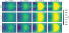 |
Fig. 3 Comparison between the 2D temperature maps of hot Jupiter GCMs in the upper row (Perna et al. 2012), and the 2D temperature maps represented with the hmℓ basis in the middle and lower rows with ℓmax = 1 and 50, respectively. The horizontal axis is longitude, the vertical axis is latitude, and the center of each map is the substellar point. For model input parameters see Table 1; for an outline of the linear algorithm used to fit maps with ℓmax = 50, see Appendix A. |
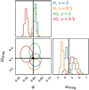 |
Fig. 4 Posterior correlations between α and ωdrag from fits of the hmℓ basis maps with ℓmax= 1 to the four hottest GCM temperature maps. The posterior distributions overlap at a few standard deviations for the values we adopt in the remainder of this work, α = 0.6 and ωdrag = 4.5 (marked with black lines). |
5.1 Reduction
We retrieved archival spitzer/IRAC observations from the Spitzer Heritage Archive3, as published in the references listed in Table 2. The reduction of these AORs follows the procedure of Demory et al. (2016a), and we refer the reader to details in that reference. We model the IRAC intra-pixel sensitivity (Ingalls et al. 2016) using a modified implementation of the BLISS (BiLinearly-Interpolated Sub-pixel Sensitivity) mapping technique (Stevenson et al. 2012).
The baseline photometric model includes the pixel response function’s FWHM along the x and y axes, which significantly reduces the level of correlated noise as shown in previous studies (e.g. Lanotte et al. 2014; Demory et al. 2016b; Demory et al. 2016a; Gillon et al. 2017; Mendonça et al. 2018). The model does not include time-dependent parameters. We vary the sampling parameters with Markov chain Monte Carlo (MCMC) in a framework already presented in Gillon et al. (2012). We run two chains of 200 000 steps each to determine the phase-curve properties at 3.6 and 4.5 μm based on the entire dataset. We trimmed the ramp in the first 30 min of the first AOR of the HAT-P-7 Channel 1 visit.
The photometry of KELT-9 b in Channel 1 is being studied in a forthcoming work by Beatty et al. (in prep.), and therefore is excluded from this work. The photometry of HD 189733 is affected by stellar variability at the mmag level requiring a special analysis unique to this object, including time-dependent parameters which we exclude from the other analyses. As such, we adopt the fully-reduced Spitzer phase curve from Knutson et al. (2012) for subsequent analysis in both Spitzer channels.
References for Spitzer phase curves presented in this work.
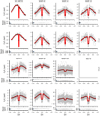 |
Fig. 5 Spitzer phase curves of the eight exoplanets (gray, binned in black) fit with the hmℓ basis (red), plotted in order of equilibrium temperature (low to high from top left to bottom right). Each planet is plotted with the IRAC Channel 1 phase curve in the first and third row and the Channel 2 phase curve in the second and fourth row (see row labels on the right side). Maximum likelihood parameters for each fit are listed in Table 3. Residuals are plotted beneath each fit with a histogram of residuals on the left. |
5.2 Analysis
In the previous section we determined that the hmℓ basis can be reduced to three fitting parameters: the redistribution factor (or greenhouse parameter) ƒ or redistribution efficiency ε, the power in the first spherical harmonic term C11, and the phase offset parameter Δϕ. In practice, these parameters respectively set: the baseline temperature field, the amplitude of the temperature variations from the day to the night side, and the hotspot offset.
Each phase curve can be fit using the hmℓ basis with the free parameters: {C11,Δϕ,ε}. We compute posterior distributions on each parameter with the No U-Turn Sampler using a STAN-like tuning schedule, implemented by (Foreman-Mackey et al. 2021). α and ωdrag are varied with tight Gaussian priors: α ~ 𝒩(0.6,0.1) and ωdrag ~ 𝒩(4.5, 1.5). By allowing these parameters to have non-zero variance, we are slightly exploring the degeneracies between parameters, especially between α and C11 which are highly correlated in fits to the phase curve with ℓmax = 1. We compute a fixed eclipse model for the planets using the best-fit planetary parameters from each paper in Table 2 using the Mandei & Agol (2002) model and implemented by Kreidberg (2015). The eclipse model incurs no new free parameters – we assume that all of the flux stemming from the phase curve signal vanishes during totality of secondary eclipse, so that the flux ratio Fp/F⋆ = 0 in eclipse.
We allow the thermal phase curves to be contaminated by sinusoidal contributions from ellipsoidal variations and Doppler beaming with unknown amplitudes but fixed phases and periods. Typical amplitudes for these sinusoidal terms are small compared to the phase variations. The most significant ellipsoidal variations affected the phase curves of WASP-103 and WASP-19.
In Fig. 5, a typical draw from the posterior distribution is plotted in red for each of the Spitzer phase curves shown in gray, and binned in black. The upper row contains observations from the 3.6 μm Channel 1, and the lower row contains 4.5 μm Channel 2 observations. The phase curves are plotted in order of increasing equilibrium temperature from left to right. The fits in red are quite good approximations to the behavior of the light curves in black. A notable exception not shown here is WASP-12, which has been claimed to have a special phase curve shape at 4.5 μm due to co-orbiting material between the planet and the star (Bell et al. 2019).
One notable phenomenon in Fig. 5 is the variation in phase curve amplitude between Spitzer channels, particularly for WASP-19 b. The difference in amplitude and phase offset between the two channels is likely because different wavelengths probe different depths and therefore different temperatures in the planet’s atmosphere. We discuss this more in Sect. 6.
Posterior distributions and parameter correlations are shown for WASP-43 b in Fig. 6. The spherical harmonic power term C11 is correlated with the dimensionless fluid parameter α, which has a tight prior.
Figure 7 shows the day side and night side temperatures derived from the Spitzer photometry of the hot Jupiters. We confirm that day side temperatures are proportional to the equilibrium temperatures as found by Schwartz & Cowan (2015). We also independently confirm the observation of Keating et al. (2019); Beatty et al. (2019) which suggested that the night side temperatures of most hot Jupiters are similar to 1100 K, irrespective of equilibrium temperature. It has been suggested that silicates and hydrocarbon hazes can produce this trend (Gao et al. 2020). We note that this trend is broken by KELT-9 b, which is hot enough to dissociate H2 molecules on its dayside, affecting the global heat transport (see, e.g.: Bell & Cowan 2018; Wong et al. 2020; Roth et al. 2021; Mansfield et al. 2020).
The best-fit hmℓ basis parameters C11 and Δϕ for both the fits to the GCM temperature maps and the Spitzer phase curves are plotted in Fig. 8. The C11 values from the fits to the hottest GCMs agree well with the results from the Spitzer phase curves. The Spitzer phase curves show a roughly linear increase with equilibrium temperature given by
 (23)
(23)
 (24)
(24)
for planetary equilibrium temperatures between 1200 K and 3100 K. The phase offset parameter Δϕ is close to zero for all Spitzer phase curves except for the two most extreme temperature cases, while all GCMs below 1500 K indicate significantly nonzero phase offsets. The rather extreme phase offset of HD 189733 b is consistent with the range observed in GCM temperature maps of similar equilibrium temperatures. The simulations and the observations are in good agreement in terms of both C11 and Δϕ where the equilibrium temperatures overlap near 2000 K.
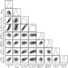 |
Fig. 6 Posterior distributions for the three derived parameters {Δϕ, C11,ε} which determine the amplitude and shape of the phase curve for WASP-43 b as observed in Spitzer IRAC 1 and 2 (3.6, 4.5 μm), with priors on {α, ωdrag}. The global α parameter is degenerate with the C11 specific to each bandpass, which introduces a cross-bandpass correlation between the two C11 parameters. |
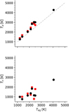 |
Fig. 7 Hemispherically-averaged day side and night side temperatures Td, Tn in Spitzer Channel 1 (red squares) and Channel 2 (black circles) as a function of planetary equilibrium temperature. These temperatures are derived by averaging the day side and night side temperature maps derived from the full phase curve fit. The hottest planet is KELT-9 b, which clearly breaks the apparent “uniform night side temperature” trend among cooler hot Jupiters noted by Keating et al. (2019). Uncertainties are smaller than the points. |
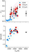 |
Fig. 8 Maximum-likelihood parameters for the spherical harmonic power coefficient C11 (upper) and hotspot offset (lower) for the full sample of GCM fits and Spitzer phase curve fits in two filter bands. Blue points are the results of fits to GCMs, circles and squares correspond to inverted and non-inverted atmospheres. Red squares and black circles represent fits to the Spitzer phase curves in filters IRAC 1 and 2, respectively. |
6 Discussion
6.1 Comparison With Bell et al. (2021)
Recently Bell et al. (2021) produced re-reduced Spitzer phase curves of many targets, including seven planets in common with this analysis. We compare their results with the ones presented in this work in Fig. 11, showing excellent agreement on the day side temperatures, indicating that the day side temperature inferences are not strongly model dependent. The two hottest planets show significantly hotter temperatures in the Bell et al. (2021) analysis than in the analysis presented here, which may be attributed to differences in the reduction process.
6.2 Temperature Forecasts For hot Jupiters
By tightly constraining the α and ωdrag parameters we have essentially fit the phase curves of each planet with a nearly identical temperature map with different relative scalings and rotations. Figure 8 shows roughly monotonic trends for the retrieved values of Δϕ and C11 as a function of the equilibrium temperature for our analysis of both GCMs and Spitzer data. These trends suggest a well-behaved sequence of Spitzer -derived temperature maps, which we show in Fig. 9. This sequence in turn suggests, to first order, a roughly universal climate state for hot Jupiters, consistent with theoretical expectations (Showman & Polvani 2011; Tsai et al. 2014).
In other words, one unified map can explain the phase variations of all of the hot Jupiters, if we rescaled all of the derived maps by the three parameters (ƒ, Δϕ and C11). We propose that most hot Jupiters should have temperature maps like Fig. 10. We can test this hypothesis with upcoming observations from the CHEOPS space telescope, which will measure a precise and time-resolved phase curve of KELT-9 b in the optical, among other planets. Deviations from this “mean hot Jupiter” temperature map could be indicative of variations in the atmospheric structure with depth, and time-varying atmospheric conditions, for example.
6.3 When To Use hmℓ to fit a phase curve
The hmℓ basis is a generalized spherical harmonic expansion representation (parabolic cylinder functions) of the temperature map of a celestial body based on solutions to the shallow water system. In this work, we have shown that spherical harmonic degrees as small as ℓmax = 1 are sufficient to approximate the temperature maps of highly irradiated, giant exoplanets, for certain values of α and ωdrag.
The shallow water framework is applicable for systems where the horizontal dimension of dynamics in the fluid far exceeds the radial one (hence the “shallow” part of the name). This is true for giant exoplanets, for example, where a few pressure scale heights in the outer parts of the atmosphere interact with light, and the bulk of the planetary radius is insulated from stellar irradiation.
The shallow water system at small spherical harmonic degrees would struggle to approximate the temperature maps of planets without atmospheres. Such worlds can have Td ≫ 0 K and Tn ≈ 0 K when synchronously rotating, and the discontinuity near the terminator could only be successfully reproduced by the hmℓ basis at large spherical harmonic degrees. We note that this challenge is not unique to the hmℓ basis, but rather a shortcoming of spherical harmonic expansion maps in general. As such, we recommend that the hmℓ basis should be applied only to planets that are likely to have atmospheres.
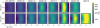 |
Fig. 9 Maximum-likelihood temperature maps for several of the hottest exoplanets, in order of increasing equilibrium temperature from left to right, where the horizontal axes are planetary longitude and vertical axes are latitude. The horizontal axis is the longitude centered on the sub stellar point, the vertical axis is latitude from pole to pole. The upper row shows the Spitzer IRAC Channel 1 (3.6 μm) inferences, the lower row shows IRAC Channel 2 (4.5 μm). The longitudinal temperature variations are constrained by the Spitzer phase curve observations while the latitudinal temperature variations are fixed at the parameterization that best describes the GCMs. |
6.4 Discrepancies Between Bandpasses
Differences between the inferred parameters across multiple filter band passes can be attributed to variations in the typical altitude probed by the photosphere of the planet at each wavelength. Table 3 shows the inferred phase curve parameters using the hmℓ basis for Spitzer IRAC Channels 1 and 2 for eight planets. The day side and night side temperatures, for example, can be significantly different between the two Spitzer band-passes. This is the case for WASP-18 b, which has a day-side integrated temperature nearly 250 K cooler in Channel 1 than Channel 2, corresponding to a difference of ≈ 10× the uncertainty on either measurement. Such differences between band passes can occur when variable opacity with wavelength determines the depth of the photosphere. The 3D nature of the planet’s atmosphere is often described with a piecewise, non-linear temperature-pressure profile with altitude (see, e.g.: Kitzmann et al. 2020), and the phase curve brightness temperatures presented here represent samples from the T–P profile weighted by the contribution function for a given bandpass.
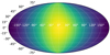 |
Fig. 10 The “universal” temperature map for hot Jupiters: scaled versions of this temperature map are consistent with both the temperature distributions in GCMs (which constrain the latitudinal distribution) and the phase curves of the hottest exoplanets (which constrain the longitudinal distribution). This map has α = 0.6 and ωdrag = 4.5 and an arbitrary scaling for ƒ, C11 and Δϕ = 0. |
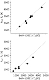 |
Fig. 11 Hemispherically-averaged day side and night side temperatures from analysis with the hmℓ framework compared with a more traditional analysis by Bell et al. (2021), showing good agreement between techniques. |
6.5 Reporting Bond Albedos and Heat Redistribution From 2D Temperature Maps
As discussed in Sect. 3, Cowan & Agol (2011b) devised a simple parameterization for the Bond albedo AB and heat redistribution efficiency parameter ε. This “0D” approach constructs a planet with a day side and night side temperature, and the relationship between those temperatures is dictated by the energy balance in the star-planet system, which is parameterized by AB and ε. We show in Sect. 3 that the Cowan & Agol (2011b) relations for these parameters can be manipulated to compute AB and ε given the temperature map of the planet.
Since the temperature maps inferred in this work are 2D, we outline a more general relationship between the full temperature map, AB, and ε in Sect. 3.4. This 2D, energy-balanced approach sets the thermal emission of a planet through its entire surface equal to the radiation incident on the planet’s day side. We adopt the resulting expression for AB throughout this work.
We also redefine the heat redistribution efficiency as the ratio of the flux emitted by the night side of the planet and the flux emitted through the day side. This definition preserves the limits ε ∈ [0,1], as in Cowan & Agol (2011b), and is straightforward to compute from both GCM outputs and hmℓ maps. The Bond albedos and heat redistribution parameters derived in this work are plotted in Fig. 12.
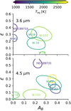 |
Fig. 12 Posterior distributions for the Bond albedos and heat redistribution efficiencies from the Spitzer phase curves of several hot exoplanets, colored by their equilibrium temperatures, in the style of Fig. 3 of Schwartz et al. (2017). Section 3 defines AB and ε for the 2D temperature maps inferred from the hmℓ basis. |
6.5.1 On The Definition Of The Bond Albedo
The Bond albedo is defined as the spherical albedo As(λ) integrated over all wavelengths, weighted by the stellar spectrum
 (25)
(25)
where I⋆(λ, T⋆) is the incoming stellar radiation. In Sect. 3.4, we express the Bond albedo assuming the brightness temperature of the planet in any finite bandpass will balance the incoming stellar radiation over all wavelengths; in other words, the planet is assumed to be a blackbody4 which reflects light with some efficiency 1 – AB. A real planet does not emit as a black body and has spectral features, and thus its brightness temperatures in finite band passes are not equivalent to the equilibrium temperature. As a result of these subtleties, (1) the AB inferred from a finite bandpass may be negative, and (2) AB estimates inferred from brightness temperatures in distinct band passes may have different values5.
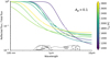 |
Fig. 13 Fraction of light reflected from the planetary surface at secondary eclipse normalized by the total flux from both reflection and thermal emission, assuming constant Ag(λ) = 0.1, after Fig. 4 of Schwartz & Cowan (2015). Black body emission is assumed for both the planet and the star. See Appendix B for details. |
6.5.2 On The Definition of The Heat Redistribution Efficiency
The heat redistribution efficiency ε as defined for 2D temperature maps in Eq. (22) is distinct from the definition in Cowan & Agol (2011b). For example, consider a planet that has a uniform dayside temperature Td and uniform nightside temperature Tn. The 0D derivation yields
 (26)
(26)
whereas the 2D approach reduces to
 (27)
(27)
These expressions are equivalent when ε0D = ε2D = 1 and Td = Tn. For imperfect recirculation efficiencies, the appearance of the day side and night side temperatures in the denominator of Eq. 26 ensures that the 0D and 2D approaches yield different efficiencies. It can be shown that the 0D efficiencies are larger than the 2D efficiencies by up to ≲ 0.24, where the maximal difference occurs for Td + Tn = 8(Td – Tn).
6.6 Reflected Light
One caveat of the analysis presented here is that we make the usual assumption that the reflected light component of the phase curve in the Spitzer bandpass is negligible. Figure 13 shows the expected contribution of reflected light to the observed, reflected and thermal emission spectrum of the planet, assuming Ag =0.1, similar to typical hot Jupiters in the Kepler bandpass (Heng & Demory 2013). Details of the calculation are provided in Appendix B.
The contribution of reflected light to the total planetary flux is on the order of a few percent for the warm Spitzer band passes for all targets in this work. Reflected light contributes significant flux at optical wavelengths for cooler exoplanets such as HD 189733 b and WASP-43 b. Joint inferences are required for the thermal emission and reflectance properties of cooler exoplanets at optical wavelengths (see, e.g.: Heng et al. 2021). Ultra-hot Jupiters such as KELT-9 b are dominated by thermal emission even at blue-optical wavelengths. Phase curves of cooler giant exoplanets from the JWST in the NIRSpec/Prism mode, for example, will be a mixture of thermal emission and reflected light that varies with wavelength. A similar conclusion on reflected light was reached by Keating & Cowan (2017).
6.7 Comparison With Traditional Spherical Harmonics
include in Appendix C calculations which indicate that the hmℓ basis reproduces GCM temperature maps more accurately than the traditional spherical harmonic  basis. We conclude that the hmℓ basis functions provide better fits to GCM temperature maps than similar
  basis functions, which may be relevant when self-consistently computing hotspot offsets and phase curve amplitudes directly from GCM temperature maps and indirectly from phase curves, as is the subject of this work.
7 Conclusion
GCM temperature maps and real photometric phase curves can be compared using the same language, which is a set of modified spherical harmonic basis functions which we call the hmℓ basis (Sect. 2)
The “0D” derivation for the Bond albedo AB and the heat redistribution efficiency ε popularized by Cowan & Agol (2011b) can be generalized when considering 2D temperature maps (Sect. 3)
There are only three free thermal parameters required to fit each phase curve in a given bandpass, (C11, Δϕ, ƒ}
We can fit GCM outputs (Sect. 4) and Spitzer phase curves (Sect. 5) with the same {α, ωdrag}, and therefore there exists one “universal” hot Jupiter map, which after scaling and rotation can matches existing hot Jupiter observations
Bond albedos, heat redistribution efficiencies, phase offsets, and day- and night-side temperatures are computed for several hot Jupiters with Spitzer phase curves (Table 3)
We confirm that reflected light from planets will contaminate the bluest wavelengths accessible to the James Webb Space Telescope, and the contamination is most severe for cooler planets
Comparisons of the hmℓ basis with the traditional
 basis suggest that GCMs are more accurately reproduced with the hmℓ basis, though the resulting phase curves are usually indistinguishable.
We offer code that computes the hmℓ maps and their phase curves efficiently called kelp, which is publicly available with implementations in Cython, theano and JAX6.
Acknowledgements.
This manuscript was carefully and thoughtfully reviewed and improved by Nicolas Cowan. This work has been carried out in the framework of the PlanetS National Centre of Competence in Research (NCCR) supported by the Swiss National Science Foundation (SNSF). We gratefully acknowledge software testing and discussions with Matthew Hooton and Adrien Deline. KH acknowledges partial financial support by a European Research Council Consolidator Grant (number 771620, project EXOKLEIN). KJ acknowledges financial support by a Hans Sigrist Foundation Ph.D Fellowship. We thank Russell Deitrick, Elsie Lee and Nathan Mayne for providing GCM output from previous publications. This research has made use of NASA’s Astrophysics Data System. This paper includes data collected by the TESS mission. Funding for the TESS mission is provided by the NASA Explorer Program. This research has made use of the VizieR catalogue access tool, CDS, Strasbourg, France (DOI: 10.26093/cds/vizier). The original description of the VizieR service was published in A&AS 143, 23. CP acknowledges financial support from a scholarship awarded by the Fonds de Recherche Québécois – Nature et Technologie (FRQNT B1X and International Internships Program – Programme de stages internationaux; Québec), a Technologies for Exo-Planetary Science (TEPS) PhD scholarship and the Vanier scholarship from the Natural Sciences and Engineering Research Council (NSERC) of Canada. We gratefully acknowledge the open source software that made this work possible: astropy (Astropy Collaboration et al. 2013, 2018), ipython (Pérez & Granger 2007), numpy (Harris et al. 2020), scipy (Virtanen et al. 2020), matplotlib (Hunter 2007), batman (Kreidberg 2015), emcee (Foreman-Mackey et al. 2013), PyMC3 (Salvatier et al. 2016), theano (Theano Development Team 2016), pymc3-ext (Foreman-Mackey et al. 2021), corner (Foreman-Mackey 2016), cython (Behnel et al. 2011), JAX (Bradbury et al. 2018).
Appendix A hmℓ linear solve
In this Appendix we outline how to reproduce a given GCM temperature map, for example, with the hmℓ basis, as done in the bottom row of Figure 3. We outline here the linear solution for the Cmℓ terms that produce hmℓ maps at arbitrary ℓmax, following the linear solve technique of Luger et al. (2019).
For all m, ℓ, one can construct the hmℓ perturbation map from Equation (2), setting each Cmℓ to a positive constant. Each 2D perturbation map is then flattened into a column vector, and each column vector is stacked with the others to produce a design matrix; this is known in the starry framework as a “pixelization matrix,” P. We stack onto this design matrix a column vector of ones to represent the mean temperature. One can then linearly solve for Q in
 (A.1)
(A.1)
where w is a weight matrix which can be assigned to sin θ in order to reproduce equatorial features and down-weight the polar regions, for example, and the matrix A is
 (A.2)
(A.2)
where I is the identity matrix and ϵ is a small positive constant. The vector of unnormalized Cmℓ coefficients c′ which reproduce a given temperature map Tinput can be found by multiplying Q by the temperature map,
 (A.3)
(A.3)
Finally we normalize each c′ by the mean of the temperature map  The resulting c vector represents each Cm,ℓ power coefficient to be passed through the hmℓ framework in order to produce the hmℓ representation of Tinput.
Appendix B Reflected light
The observed flux from an exoplanet is the sum of the thermal emission spectrum and the reflected starlight,
 (B.1)
(B.1)
The thermal emission component is written in Equation (3). The reflected light component is defined as a function of the geometric albedo at a given wavelength
 (B.2)
(B.2)
where Ψ(ξ) is the integral phase function and F⋆(λ) is the stellar emission spectrum.
The ratio of the reflected light spectrum observed at secondary eclipse (ξ = 0) to the total planetary flux is given by
 (B.3)
(B.3)
 (B.4)
(B.4)
In Figure 13, we compute each curve by solving the equation above with the corresponding planetary and stellar parameters, assuming Ag(λ) = 0.1 is constant with wavelength. Note that the thermal emission component is computed using the temperature map inferred from the Spitzer Channel 2 phase curves, though as discussed in Section 6.4, the observed, brightness temperature of the planet is a function of wavelength.
Appendix C Comparison with traditional spherical harmonics
In Figure C.1, we select a model with three free parameters in both the hmℓ and  representations to solve linearly (see our Appendix A for the mathematical approach). The differences between hmℓ and
  can be as large as 400 K peak-to-peak. The χ2 between both the hmℓ and
  representations compared with the GCM temperature map is labelled on each hmℓ and
  map. We note that the χ2 is significantly smaller for each hmℓ representation than the corresponding
  representation with the same number of free parameters. This indicates that the GCM temperature maps are more accurately reproduced by the hmℓ basis than the
  basis, even though the phase curves produced by either the hmℓ or
  solutions are nearly indistinguishable.
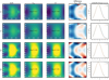 |
Fig. C.1 The four hottest GCM temperature maps (first column), the best-fit linear solutions with a low-order hmℓ representation (second column), the fits with low-order ordinary spherical harmonic representation (third column, labeled |

References
- Astropy Collaboration (Robitaille, T. P., et al.) 2013, A&A, 558, A33 [NASA ADS] [CrossRef] [EDP Sciences] [Google Scholar]
- Astropy Collaboration (Price-Whelan, A. M., et al.) 2018, AJ, 156, 123 [Google Scholar]
- Beatty, T. G., Marley, M. S., Gaudi, B. S., et al. 2019, AJ, 158, 166 [Google Scholar]
- Behnel, S., Bradshaw, R., Citro, C., et al. 2011, Comput. Sci. Eng., 13, 31 [Google Scholar]
- Bell, T. J., & Cowan, N. B. 2018, ApJ, 857, L20 [Google Scholar]
- Bell, T. J., Zhang, M., Cubillos, P. E., et al. 2019, MNRAS, 489, 1995 [Google Scholar]
- Bell, T. J., Dang, L., Cowan, N. B., et al. 2021, MNRAS, 504, 3316 [NASA ADS] [CrossRef] [Google Scholar]
- Bradbury, J., Frostig, R., Hawkins, P., et al. 2018, JAX: composable transformations of Python+NumPy programs [Google Scholar]
- Braginsky, S. I. 1998, Earth Planets Space, 50, 641 [NASA ADS] [CrossRef] [Google Scholar]
- Cho, J. Y. K., Menou, K., Hansen, B. M. S., & Seager, S. 2008, ApJ, 675, 817 [NASA ADS] [CrossRef] [Google Scholar]
- Cowan, N. B., & Agol, E. 2008, ApJ, 678, L129 [Google Scholar]
- Cowan, N. B., & Agol, E. 2011a, ApJ, 726, 82 [NASA ADS] [CrossRef] [Google Scholar]
- Cowan, N. B., & Agol, E. 2011b, ApJ, 729, 54 [Google Scholar]
- Cowan, N. B., & Fujii, Y. 2018, Mapping Exoplanets, eds. H. J. Deeg & J. A. Belmonte, 147 [Google Scholar]
- Cowan, N. B., Fuentes, P. A., & Haggard, H. M. 2013, MNRAS, 434, 2465 [NASA ADS] [CrossRef] [Google Scholar]
- Cowan, N. B., Chayes, V., Bouffard, É., Meynig, M., & Haggard, H. M. 2017, MNRAS, 467, 747 [NASA ADS] [Google Scholar]
- de Wit, J., Gillon, M., Demory, B. O., & Seager, S. 2012, A&A, 548, A128 [NASA ADS] [CrossRef] [EDP Sciences] [Google Scholar]
- Demory, B.-O., Gillon, M., de Wit, J., et al. 2016a, Nature, 532, 207 [NASA ADS] [CrossRef] [Google Scholar]
- Demory, B.-O., Gillon, M., Madhusudhan, N., & Queloz, D. 2016b, MNRAS, 455, 2018 [NASA ADS] [CrossRef] [Google Scholar]
- Foreman-Mackey, D. 2016, J. Open Source Softw, 1, 24 [NASA ADS] [CrossRef] [Google Scholar]
- Foreman-Mackey, D., Hogg, D. W., Lang, D., & Goodman, J. 2013, PASP, 125, 306 [Google Scholar]
- Foreman-Mackey, D., Luger, R., Agol, E., et al. 2021, J. Open Source Softw., 6, 3285 [NASA ADS] [CrossRef] [Google Scholar]
- Gao, P., Thorngren, D. P., Lee, E. K. H., et al. 2020, Nat. Astron., 4, 951 [NASA ADS] [CrossRef] [Google Scholar]
- Gill, A. E. 1980, Q. J. R. Meteorol. Soc., 106, 447 [NASA ADS] [CrossRef] [Google Scholar]
- Gillon, M., Demory, B. O., Benneke, B., et al. 2012, A&A, 539, A28 [NASA ADS] [CrossRef] [EDP Sciences] [Google Scholar]
- Gillon, M., Demory, B. O., Lovis, C., et al. 2017, A&A, 601, A117 [NASA ADS] [CrossRef] [EDP Sciences] [Google Scholar]
- Gilman, P. A. 2000, ApJ, 544, L79 [NASA ADS] [CrossRef] [Google Scholar]
- Guillot, T. 2010, A&A, 520, A27 [NASA ADS] [CrossRef] [EDP Sciences] [Google Scholar]
- Hansen, B. M. S. 2008, ApJS, 179, 484 [NASA ADS] [CrossRef] [Google Scholar]
- Harris, C. R., Millman, K. J., van der Walt, S. J., et al. 2020, Nature, 585, 357 [NASA ADS] [CrossRef] [Google Scholar]
- Heng, K., & Demory, B.-O. 2013, ApJ, 777, 100 [NASA ADS] [CrossRef] [Google Scholar]
- Heng, K., & Showman, A. P. 2015, Ann. Rev. Earth Planet. Sci., 43, 509 [Google Scholar]
- Heng, K., & Spitkovsky, A. 2009, ApJ, 703, 1819 [NASA ADS] [CrossRef] [Google Scholar]
- Heng, K., & Workman, J. 2014, ApJS, 213, 27 [CrossRef] [Google Scholar]
- Heng, K., Morris, B. M., & Kitzmann, D. 2021, Nat. Astron., 5, 1001 [NASA ADS] [CrossRef] [Google Scholar]
- Hu, R., Demory, B.-O., Seager, S., Lewis, N., & Showman, A. P. 2015, ApJ, 802, 51 [Google Scholar]
- Hunter, J. D. 2007, Comput. Sci. Eng., 9, 90 [NASA ADS] [CrossRef] [Google Scholar]
- Husser, T.-O., Wende-von Berg, S., Dreizler, S., et al. 2013, A&A, 553, A6 [NASA ADS] [CrossRef] [EDP Sciences] [Google Scholar]
- Ingalls, J. G., Krick, J. E., Carey, S. J., et al. 2016, AJ, 152, 44 [NASA ADS] [CrossRef] [Google Scholar]
- Keating, D., & Cowan, N. B. 2017, ApJ, 849, L5 [Google Scholar]
- Keating, D., Cowan, N. B., & Dang, L. 2019, Nat. Astron., 3, 1092 [NASA ADS] [CrossRef] [Google Scholar]
- Kitzmann, D., Heng, K., Oreshenko, M., et al. 2020, ApJ, 890, 174 [Google Scholar]
- Knutson, H. A., Charbonneau, D., Allen, L. E., et al. 2007, Nature, 447, 183 [NASA ADS] [CrossRef] [Google Scholar]
- Knutson, H. A., Lewis, N., Fortney, J. J., et al. 2012, ApJ, 754, 22 [NASA ADS] [CrossRef] [Google Scholar]
- Kreidberg, L. 2015, PASP, 127, 1161 [Google Scholar]
- Kreidberg, L., Line, M. R., Parmentier, V., et al. 2018, AJ, 156, 17 [NASA ADS] [CrossRef] [Google Scholar]
- Lanotte, A. A., Gillon, M., Demory, B. O., et al. 2014, A&A, 572, A73 [NASA ADS] [CrossRef] [EDP Sciences] [Google Scholar]
- Longuet-Higgins, M. S. 1967, J. Fluid Mech., 29, 781 [NASA ADS] [CrossRef] [Google Scholar]
- Longuet-Higgins, M. S. 1968, Phil. Trans. R. Soc. Lond. A, 262, 511 [CrossRef] [Google Scholar]
- López-Morales, M., & Seager, S. 2007, ApJ, 667, L191 [CrossRef] [Google Scholar]
- Luger, R., Agol, E., Foreman-Mackey, D., et al. 2019, AJ, 157, 64 [Google Scholar]
- Madhusudhan, N. 2019, ARA&A, 57, 617 [NASA ADS] [CrossRef] [Google Scholar]
- Majeau, C., Agol, E., & Cowan, N. B. 2012, ApJ, 747, L20 [NASA ADS] [CrossRef] [Google Scholar]
- Mandel, K., & Agol, E. 2002, ApJ, 580, L171 [Google Scholar]
- Mansfield, M., Bean, J. L., Stevenson, K. B., et al. 2020, ApJ, 888, L15 [Google Scholar]
- Marley, M. S., Gelino, C., Stephens, D., Lunine, J. I., & Freedman, R. 1999, ApJ, 513, 879 [NASA ADS] [CrossRef] [Google Scholar]
- Matsuno, T. 1966, J. Meteorol. Soc. Jpn., 44, 25 [NASA ADS] [CrossRef] [Google Scholar]
- Maxted, P. F. L., Anderson, D. R., Doyle, A. P., et al. 2013, MNRAS, 428, 2645 [NASA ADS] [CrossRef] [Google Scholar]
- Mendonça, J. M., Malik, M., Demory, B.-O., & Heng, K. 2018, AJ, 155, 150 [Google Scholar]
- Parmentier, V., & Crossfield, I. J. M. 2018, Exoplanet Phase Curves: Observations and Theory, eds. H. J. Deeg, & J. A. Belmonte, 116 [Google Scholar]
- Pérez, F., & Granger, B. E. 2007, Computing in Science and Engineering, 9, 21 [CrossRef] [Google Scholar]
- Perna, R., Heng, K., & Pont, F. 2012, ApJ, 751, 59 [NASA ADS] [CrossRef] [Google Scholar]
- Rauscher, E., Suri, V., & Cowan, N. B. 2018, AJ, 156, 235 [NASA ADS] [CrossRef] [Google Scholar]
- Roth, A., Drummond, B., Hébrard, E., et al. 2021, MNRAS, 505, 4515 [NASA ADS] [CrossRef] [Google Scholar]
- Salvatier, J., Wiecki, T. V., & Fonnesbeck, C. 2016, PeerJ Comput. Sci., 2, e55 [Google Scholar]
- Schwartz, J. C., & Cowan, N. B. 2015, MNRAS, 449, 4192 [NASA ADS] [CrossRef] [Google Scholar]
- Schwartz, J. C., Kashner, Z., Jovmir, D., & Cowan, N. B. 2017, ApJ, 850, 154 [Google Scholar]
- Seager, S. 2010, Exoplanets [Google Scholar]
- Showman, A. P., & Polvani, L. M. 2011, ApJ, 738, 71 [Google Scholar]
- Stevenson, K. B., Harrington, J., Fortney, J. J., et al. 2012, ApJ, 754, 136 [Google Scholar]
- Stevenson, K. B., Désert, J.-M., Line, M. R., et al. 2014, Science, 346, 838 [Google Scholar]
- Theano Development Team 2016, arXiv e-prints, [arXiv:abs/1605.02688] [Google Scholar]
- Tsai, S.-M., Dobbs-Dixon, I., & Gu, P.-G. 2014, ApJ, 793, 141 [NASA ADS] [CrossRef] [Google Scholar]
- Virtanen, P., Gommers, R., Oliphant, T. E., et al. 2020, Nat. Methods, 17, 261 [Google Scholar]
- Wong, I., Knutson, H. A., Lewis, N. K., et al. 2015, ApJ, 811, 122 [NASA ADS] [CrossRef] [Google Scholar]
- Wong, I., Knutson, H. A., Kataria, T., et al. 2016, ApJ, 823, 122 [NASA ADS] [CrossRef] [Google Scholar]
- Wong, I., Shporer, A., Kitzmann, D., et al. 2020, AJ, 160, 88 [Google Scholar]
- Wong, I., Kitzmann, D., Shporer, A., et al. 2021, AJ, 162, 127 [NASA ADS] [CrossRef] [Google Scholar]
Note that this definition includes the Bond albedo, which is different from Cowan & Agol (2011b) who use T0  to represent the irradiation temperature.
We note that this definition of a “blackbody” is somewhat inconsistent, since a blackbody should be perfectly absorbing with AB = 0.
In this sense, the “AB” we discuss in this manuscript is a function of wavelength, unlike its definition in Eq. (25).
All Tables
All Figures
|
Fig. 1 Four montages of the first several terms in the generalized spherical harmonic expansion of the temperature map in the hmℓ basis. Each montage corresponds to a different combination of α and ωdrag, labeled in the upper right of each quadrant. Each map shows the temperature perturbation (purple to yellow is cold to hot) as a function of latitude and longitude (shown in Moll weide projections such that the sub stellar longitude is in the center of the plot). The m = 0 terms are always zero. The even-ℓ terms are asymmetric about the equator and therefore do not represent typical GCM results in equilibrium, so we keep all even-ℓ power coefficients fixed to zero in the subsequent fits (this approach assumes edge-on orbits, for exceptions see Cowan et al. 2017). In the upper two quadrants, when ωdrag is set to a smaller value, the chevron shape becomes more pronounced. In the two quadrants on the right, when the α is set to a larger value, the concentration of heat near the equator is more pronounced. |
| In the text | |
|
Fig. 2 Lower limit on Td/Tirr (curve) for producing negative Bond albedos. For comparison, empirically obtained values of Td/Tirr from Wong et al. (2021) are shown; the uncertainties on these values (not shown for plot clarity) are between 2% and 5%. |
| In the text | |
|
Fig. 3 Comparison between the 2D temperature maps of hot Jupiter GCMs in the upper row (Perna et al. 2012), and the 2D temperature maps represented with the hmℓ basis in the middle and lower rows with ℓmax = 1 and 50, respectively. The horizontal axis is longitude, the vertical axis is latitude, and the center of each map is the substellar point. For model input parameters see Table 1; for an outline of the linear algorithm used to fit maps with ℓmax = 50, see Appendix A. |
| In the text | |
|
Fig. 4 Posterior correlations between α and ωdrag from fits of the hmℓ basis maps with ℓmax= 1 to the four hottest GCM temperature maps. The posterior distributions overlap at a few standard deviations for the values we adopt in the remainder of this work, α = 0.6 and ωdrag = 4.5 (marked with black lines). |
| In the text | |
|
Fig. 5 Spitzer phase curves of the eight exoplanets (gray, binned in black) fit with the hmℓ basis (red), plotted in order of equilibrium temperature (low to high from top left to bottom right). Each planet is plotted with the IRAC Channel 1 phase curve in the first and third row and the Channel 2 phase curve in the second and fourth row (see row labels on the right side). Maximum likelihood parameters for each fit are listed in Table 3. Residuals are plotted beneath each fit with a histogram of residuals on the left. |
| In the text | |
|
Fig. 6 Posterior distributions for the three derived parameters {Δϕ, C11,ε} which determine the amplitude and shape of the phase curve for WASP-43 b as observed in Spitzer IRAC 1 and 2 (3.6, 4.5 μm), with priors on {α, ωdrag}. The global α parameter is degenerate with the C11 specific to each bandpass, which introduces a cross-bandpass correlation between the two C11 parameters. |
| In the text | |
|
Fig. 7 Hemispherically-averaged day side and night side temperatures Td, Tn in Spitzer Channel 1 (red squares) and Channel 2 (black circles) as a function of planetary equilibrium temperature. These temperatures are derived by averaging the day side and night side temperature maps derived from the full phase curve fit. The hottest planet is KELT-9 b, which clearly breaks the apparent “uniform night side temperature” trend among cooler hot Jupiters noted by Keating et al. (2019). Uncertainties are smaller than the points. |
| In the text | |
|
Fig. 8 Maximum-likelihood parameters for the spherical harmonic power coefficient C11 (upper) and hotspot offset (lower) for the full sample of GCM fits and Spitzer phase curve fits in two filter bands. Blue points are the results of fits to GCMs, circles and squares correspond to inverted and non-inverted atmospheres. Red squares and black circles represent fits to the Spitzer phase curves in filters IRAC 1 and 2, respectively. |
| In the text | |
|
Fig. 9 Maximum-likelihood temperature maps for several of the hottest exoplanets, in order of increasing equilibrium temperature from left to right, where the horizontal axes are planetary longitude and vertical axes are latitude. The horizontal axis is the longitude centered on the sub stellar point, the vertical axis is latitude from pole to pole. The upper row shows the Spitzer IRAC Channel 1 (3.6 μm) inferences, the lower row shows IRAC Channel 2 (4.5 μm). The longitudinal temperature variations are constrained by the Spitzer phase curve observations while the latitudinal temperature variations are fixed at the parameterization that best describes the GCMs. |
| In the text | |
|
Fig. 10 The “universal” temperature map for hot Jupiters: scaled versions of this temperature map are consistent with both the temperature distributions in GCMs (which constrain the latitudinal distribution) and the phase curves of the hottest exoplanets (which constrain the longitudinal distribution). This map has α = 0.6 and ωdrag = 4.5 and an arbitrary scaling for ƒ, C11 and Δϕ = 0. |
| In the text | |
|
Fig. 11 Hemispherically-averaged day side and night side temperatures from analysis with the hmℓ framework compared with a more traditional analysis by Bell et al. (2021), showing good agreement between techniques. |
| In the text | |
|
Fig. 12 Posterior distributions for the Bond albedos and heat redistribution efficiencies from the Spitzer phase curves of several hot exoplanets, colored by their equilibrium temperatures, in the style of Fig. 3 of Schwartz et al. (2017). Section 3 defines AB and ε for the 2D temperature maps inferred from the hmℓ basis. |
| In the text | |
|
Fig. 13 Fraction of light reflected from the planetary surface at secondary eclipse normalized by the total flux from both reflection and thermal emission, assuming constant Ag(λ) = 0.1, after Fig. 4 of Schwartz & Cowan (2015). Black body emission is assumed for both the planet and the star. See Appendix B for details. |
| In the text | |
|
Fig. C.1 The four hottest GCM temperature maps (first column), the best-fit linear solutions with a low-order hmℓ representation (second column), the fits with low-order ordinary spherical harmonic representation (third column, labeled |
| In the text | |
Current usage metrics show cumulative count of Article Views (full-text article views including HTML views, PDF and ePub downloads, according to the available data) and Abstracts Views on Vision4Press platform.
Data correspond to usage on the plateform after 2015. The current usage metrics is available 48-96 hours after online publication and is updated daily on week days.
Initial download of the metrics may take a while.