| Issue |
A&A
Volume 659, March 2022
|
|
|---|---|---|
| Article Number | A79 | |
| Number of page(s) | 28 | |
| Section | Extragalactic astronomy | |
| DOI | https://doi.org/10.1051/0004-6361/202141400 | |
| Published online | 10 March 2022 | |
HARMONI view of the host galaxies of active galactic nuclei around cosmic noon
Resolved stellar morpho-kinematics and the MBH − σ⋆ relation
1
Instituto de Astrofísica de Canarias, C/ Vía Láctea s/n, 38205 La Laguna, Tenerife, Spain
e-mail: begona.garcia@iac.es
2
Departamento de Astrofísica, Universidad de La Laguna, 38200 La Laguna, Tenerife, Spain
3
Leiden Observatory, Leiden University, PO Box 9513, 2300 RA Leiden, The Netherlands
4
Centro de Astrobiología (CSIC-INTA), Ctra. de Ajalvir, Km 4, 28850 Torrejón de Ardoz, Madrid, Spain
5
Department of Physics, Denys Wilkinson Building, Keble Road, University of Oxford, OX1 3RH Oxford, UK
6
Institute of Space Sciences (ICE, CSIC), Campus UAB, Carrer de Can Magrans, s/n, 08193 Barcelona, Spain
7
Institut d’Estudis Espacials de Catalunya (IEEC), 08034 Barcelona, Spain
Received:
27
May
2021
Accepted:
22
November
2021
Context. The formation and evolution of galaxies appear linked to the growth of supermassive black holes, as evidenced by empirical scaling relations in nearby galaxies. Understanding this co-evolution over cosmic time requires the revelation of the dynamical state of galaxies and the measurement of the mass of their central black holes (MBH) at a range of cosmic distances. Bright active galactic nuclei (AGNs) are ideal for this purpose.
Aims. The High Angular Resolution Monolithic Optical and Near-infrared Integral field spectrograph (HARMONI), the first light integral-field spectrograph for the Extremely Large Telescope, will transform visible and near-infrared ground-based astrophysics thanks to its advances in sensitivity and angular resolution. We aim to analyse the capabilities of HARMONI to reveal the stellar morpho-kinematic properties of the host galaxies of AGNs at about cosmic noon.
Methods. We made use of the simulation pipeline for HARMONI (HSIM) to create mock observations of representative AGN host galaxies at redshifts around cosmic noon. We used observations taken with the Multi Unit Spectroscopic Explorer of nearby galaxies showing different morphologies and dynamical stages combined with theoretical AGN spectra to create the target inputs for HSIM.
Results. According to our simulations, an on-source integration time of three hours should be enough to measure the MBH and to trace the morphology and stellar kinematics of the brightest host galaxies of AGNs beyond cosmic noon. For host galaxies with stellar masses < 1011 M⊙, longer exposure times are mandatory to spatially resolve the stellar kinematics.
Key words: instrumentation: high angular resolution / instrumentation: spectrographs / quasars: general / galaxies: kinematics and dynamics
© ESO 2022
1. Introduction
The formation and evolution of galaxies result from the hierarchical assembly across cosmic time. Besides, the empirical relations between large-scale properties of galaxies (e.g. bulge mass, stellar velocity dispersion, etc.) and the mass of their central supermassive black holes (SMBH) suggest a co-growth scenario (see e.g. Kormendy & Ho 2013 for a review). To constrain models and provide a comprehensive picture of the formation and evolution of galaxies, it is necessary to study the change of the scaling relations between SMBHs and their host galaxies over cosmic time. A lack of change will suggest feedback mechanisms controlling the co-growth (e.g. Di Matteo et al. 2005), while an evolution will point to a non-causal origin that will accidentally result after several interactions and mergers (e.g. Jahnke & Macciò 2011).
Both star formation and nuclear activity peak at a redshift in the 1.5 ≤ z ≤ 2 range (e.g. Madau & Dickinson 2014; Aird et al. 2015), a period often referred to as ‘cosmic noon’. A proper cosmic period to study the evolution of the scaling relations supporting the co-growth scenario should include this highest activity ridge in the Universe’s timeline. Such study requires an estimation of both the mass of central SMBHs (MBH) and the properties of the host galaxies (e.g. luminosity, size, morphology, stellar velocity dispersion, etc.) for a representative sample of objects at different redshifts.
Estimating MBH over cosmic time can be done by observing active galactic nuclei (AGNs) spectra and applying the single epoch virial method (e.g. Kaspi et al. 2000; McLure & Jarvis 2002). It assumes that the motions of the gas surrounding the black hole (i.e. the broad-line region, BLR) are virialised (e.g. Shen 2013). The procedure uses the empirical relation between the BLR size and the AGN continuum luminosity (e.g. Peterson et al. 2004) to approach MBH from parameters easily measured from AGN type 1 spectra. For example, using the Hβ emission line (see Vestergaard & Peterson 2006):
![$$ \begin{aligned} \log \left(\frac{M_{\rm BH}}{M_{\odot }}\right) =&(6.67 \pm 0.03)\nonumber \\& + \log \left(\left[\frac{FWHM(\mathrm{H}\beta )}{1000\,\mathrm{km\,s^{-1}}}\right]^{2} \left[\frac{L(\mathrm{H}\beta )}{10^{42}\,\mathrm{erg\,s^{-1}}}\right]^{0.63}\right), \end{aligned} $$](/articles/aa/full_html/2022/03/aa41400-21/aa41400-21-eq1.gif)
where FWHM(Hβ) and L(Hβ) are the full width at half maximum and luminosity, respectively, of the broad component of Hβ (see e.g. Shen et al. 2011 for other simple relations connecting emission lines and continuum luminosities and MBH). The empirical correlation found between the BLR kinematics and the ionisation state of the narrow-line region (NLR) has extended the MBH estimation to type 2 AGNs. This approach only requires us to measure the narrow line luminosities of [O III] and Hβ (Baron & Ménard 2019). We note that around cosmic noon, the Hβ, Hα, [O III]λλ4959, 5007, and [NII]λλ6548, 6584 emission lines (i.e. the traditional NLR and BLR tracers) are redshifted into the near-infrared range.
The single epoch virial method requires high signal-to-noise ratio (S/N) spectra (e.g. Marziani & Sulentic 2012). The most luminous quasi-stellar objects (QSOs) are then ideal to determine MBH across cosmic time. However, bright QSOs hide their underlying galaxies with contrasts ranging from 10−1 to 10−3 (e.g. Floyd et al. 2004). Hence, the simultaneous determination of MBH and galaxy parameters requires a compromise between the S/N of the AGN spectrum and its host galaxy spectra to control uncertainties. An efficient procedure for a proper de-blending will benefit that compromise (see e.g. García-Lorenzo et al. 2005; Vayner et al. 2016; Husemann et al. 2016; Rupke et al. 2017; Varisco et al. 2018).
The deviations of nearby mergers and bulgeless galaxies from the host-scaling relations with MBH (see e.g. Kormendy & Ho 2013 and references therein) indicate that controlling the morphology of the AGN hosts is essential when studying the evolution of scaling relations with redshift. Besides this, the stellar velocity dispersion (σ⋆) is the most fundamental parameter linking galaxies and SMBHs (Shankar et al. 2016; Marsden et al. 2020). Moreover, only the MBH − σ⋆ relation holds to all galaxy types, from dwarfs to the most massive galaxies (e.g. van den Bosch 2016), although with deviations for evolved interactions (e.g. Kormendy & Ho 2013; Saglia et al. 2016). Then, unveiling the stellar dynamical state of galaxies over cosmic time is crucial to a complete understanding of the evolution of galaxies in the framework of the co-growth scenario.
Integral field spectroscopic (IFS) surveys have extensively characterised the stellar (e.g. Falcón-Barroso et al. 2017; Stark et al. 2018; Fraser-McKelvie et al. 2021) and ionised gas (e.g. García-Lorenzo et al. 2015; Stark et al. 2018; den Brok et al. 2020) kinematics of nearby galaxies (z < 0.1) for a broad range of masses (M⋆ ∼ 108 − 1012 M⊙) and morphological types. Galaxies over z > 0.1 have scarcely been studied using IFS so far, focusing on the gaseous component to trace their kinematic evolution (Wisnioski et al. 2015; Contini et al. 2016; Förster Schreiber et al. 2018; Förster Schreiber & Wuyts 2020; Sharma et al. 2021). These studies reveal that rotation dominates the gas kinematics in many galaxies from cosmic noon. However, gas kinematics (even more in AGN hosts) is complex, with features of inflows, outflows, turbulence, clumps, and so on. Instead, the stellar component is a good tracer of the gravitational potential of galaxies. Beyond the local Universe (z > 0.1), spatially resolved stellar kinematics has barely been explored through IFS, reporting velocity fields consistent with rotating stellar disks (Guérou et al. 2017). Close to or beyond the cosmic noon, there are only σ⋆ measurements from integrated or stacked spectra of massive quiescent galaxies (e.g. Mendel et al. 2020; Esdaile et al. 2021; van der Wel et al. 2021 and references therein). The limitation on collecting power and spatial resolution of the current IFS instruments (e.g. Multi-Espectrógrafo en Gran Telescopio Canarias (GTC) de Alta Resolución para Astronomía (MEGARA1) at the 10-m GTC, the OH-Suppressing Infrared Integral Field Spectrograph (OSIRIS2) at the 10-m Keck telescope, the K-band Multi Object Spectrograph (KMOS3) or the Multi Unit Spectroscopic Explorer (MUSE4) at the 8-m Very Large Telescope (VLT), etc.) are the causes behind this lack of resolved stellar dynamics of galaxies around cosmic noon. Only the new generation of the 30−40 metre-class telescopes will allow the resolving of the stellar kinematics of active and non-active galaxies around cosmic noon.
In this work, we explored the capabilities of the High Angular Resolution Monolithic Optical and Near-infrared Integral field spectrograph (HARMONI, Thatte et al. 2016, 2020) on the Extremely Large Telescope5 (ELT) to reveal the morphological and stellar dynamical state of AGN host galaxies and to trace the cosmic evolution of the scaling relations connecting the host parameters with the mass of their central SMBHs. In Sect. 2, we describe the instrument and its different configurations to identify an optimal setup for observing AGNs and their hosts. In Sect. 3, we describe the procedure of generating inputs for the simulation pipeline and the mock HARMONI observations. The analysis and discussion are presented in Sect. 4. Section 5 summarises the main conclusions. In the following, we assume a standard ΛCDM model with H0 = 67.9 km s−1 Mpc−1, ΩM = 0.31 and ΩΛ = 0.69 (Planck Collaboration XIII 2016).
2. HARMONI
HARMONI6 will provide the first light spectroscopic capability to the ELT (see e.g. Thatte et al. 2016, 2020). HARMONI was conceived as a workhorse instrument to support a wide variety of science programmes (see e.g. Arribas et al. 2010; Thatte et al. 2016, 2020) and address many of the key science cases for the ELT7.
HARMONI includes single conjugated and laser tomography adaptive optics (SCAO and LTAO, respectively) systems to compensate the atmospheric turbulence, although seeing-limited observations are also available. SCAO will provide an excellent image quality (< 20% degradation of the telescope point-spread function; PSF) using a single, bright (J < 14) natural star reference located up to 15 arcsec from the science target. LTAO will compensate the atmospheric turbulence (∼30% Strehl in K band), with 50%–90% sky coverage. This will be done by using six laser guide stars and a reference natural star (J < 19) within up to 1 arcmin radius of the science field. HARMONI will have a similar angular resolution to the Atacama Large Millimeter/submillimeter Array (ALMA8) and comparable sensitivity to the James Webb Space Telescope (JWST9) at wavelengths < 2.5 μm, which perfectly complement each other due to many synergies. At the time of writing, the development of HARMONI is in the final design phase, with the first light scheduled for the end of 2026. In this section, we go through the multiple configurations of HARMONI with the aim of identifying the optimal setup to observe AGNs with a signal to noise and resolution that permit us to study galaxy black hole co-evolution over cosmic time.
2.1. Spatial scales and field of view
The size of the galaxies over cosmic time varies: Reff (kpc) = Bz (1 + z)βz, where Bz and βz parameters depend on stellar mass and galaxy type (van der Wel et al. 2014), and Reff is the effective radius. For redshift 2.75 > z > 0.75, the average sizes range between 1.3 ≤ Reff ≤ 2.9 kpc and 3 ≤ Reff ≤ 5 kpc for early- and late-type objects, respectively (see Table 2 in van der Wel et al. 2014), with AGN hosts lying in-between (Silverman et al. 2019). These numbers correspond to full (i.e. 2 × Reff) angular sizes in the ∼0.3−1.3 arcsec range. Moreover, many AGN hosts show gas outflows, typically extending over Reff at z > 0.6 (e.g. Brusa et al. 2016; Vayner et al. 2017; Schreiber et al. 2019), sometimes reaching even a few Reff (e.g. Nesvadba et al. 2006; Harrison et al. 2012; Leung et al. 2019). Considering this, we need a field of view (FoV) of a few times the largest angular size expected for these high-redshift AGN host+outflows, that is a few arcsec.
HARMONI offers four different spatial configurations (see Table 1) providing spectra of more than 31 000 spatial positions arranged in a rectangular array of 152 × 204 spaxels. The two finer spatial scales will provide high spatial resolution, but their FoVs are smaller than some of the most powerful outflows observed in AGNs (e.g. Nesvadba et al. 2006; Harrison et al. 2012; Leung et al. 2019). On the contrary, the FoV of the two coarser scales fits the expected size of the most extended outflows, with physical resolutions comparable to surveys of nearby galaxies like the Calar Alto Legacy Integral Field Area (CALIFA) survey (Sánchez et al. 2016), the Mapping Nearby Galaxies at APO (MANGA) survey (Bundy et al. 2015), or the Sydney-Australian-Astronomical-Observatory Multi-object Integral-Field Spectrograph (SAMI) survey (Croom et al. 2012). Moreover, the coarser scales also simultaneously sample the background allowing on-frame sky subtraction. We thus selected the 20 × 20 mas2 scale for our HARMONI simulations of AGN+host galaxies. This scale provides the best sensitivity among the four HARMONI spatial scales (Zieleniewski et al. 2015), and it preserves, at a fixed S/N threshold, better spatial resolution than the 30 × 60 mas2 scale. Some results on mock HARMONI observations of QSO+host galaxies using the 30 × 60 mas2 spatial scale were presented in García-Lorenzo et al. (2019).
HARMONI spatial configurations.
2.2. Spectral resolutions and gratings
To optimise the ELT+HARMONI observing time, it is desirable to have all the required information in a single shot, that is, a grating whose wavelength coverage includes both emission lines and stellar features to measure the MBH and σ⋆ parameters. HARMONI will provide three resolving powers (R = λ/Δλ of ∼3200, ∼7000, and ∼18 000) in different bands (see Fig. 1). Depending on the redshift of the target, the relevant spectral features will be shifted to different wavelengths. Figure 1 includes the wavelength of some emission and absorption lines as a function of redshift.
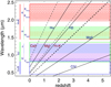 |
Fig. 1. Key spectral features to measure MBH and σ⋆ observable at each HARMONI band as a function of the redshift. Black solid and dashed lines correspond to emission (i.e. CIV, MgII, Hβ, and Hα) and absorption (i.e. CaIIH+K, MgI, and CaII) features, respectively. The low-resolution bands correspond to the wavelength range between blue (V + R), green (I + z + J), and red (H + K) rectangles. Purple (I + z), blue (J), green (H), and red (K) filled rectangles mark the wavelength range of medium-resolution gratings. Hatch patterns mark the high-resolution bands: purple, striped, inclined: Zhigh; orange striped: Hhigh; red, striped; inclined: Kshort; and red, dashed, striped: Klong. |
The HARMONI high spectral resolution bands will provide accurate estimates of the stellar velocity dispersion, with a spectral resolution of ∼1 Å (or σ⋆ ∼ 7 km s−1) at 1.92 μm. However, only for the K bands (i.e. Kshort, and Klong) could stellar and broad ionised gas features be simultaneously observed (i.e. from Hβ to MgI lines) for objects at z ⪆ 3.2. The HARMONI medium-resolution bands can sample the Hβ-MgI region for AGNs in the ∼0.6 to ∼3.7 redshift range with a spectral resolution of about 2.7 Å (or σ⋆ ∼ 18 km s−1). Nevertheless, the simultaneous observation of the MgI stellar feature and Hβ emission line is unfeasible using these medium-resolution gratings for objects in two redshift gaps (i.e. ∼[1.5−2.0], and ∼[2.5−3.1]). The HARMONI low-resolution gratings enable us to observe a wide spectral range including several emission and absorption features from nearby to high-redshift objects (see Fig. 1). Indeed, the estimation of MBH and σ⋆ is possible with HARMONI low-resolution gratings for AGNs in the 0 ≤ z ≤ 3.7 range observing the Hβ-MgI region (there is only a gap for objects in the ∼[1.7−2.0] redshift range).
We note that a resolution of ∼3200 corresponds to a Δλ of ∼6 Å (or σ⋆ ∼ 40 km s−1) at 1.92 μm. Current optical spectroscopic surveys of nearby galaxies measure stellar velocity dispersions with spectral resolutions that range from 30 to 140 km s−1 (see e.g. The Baryon Oscillation Spectroscopic Survey (BOSS), Thomas et al. 2013; MANGA, Law et al. 2016; SAMI, van de Sande et al. 2017; CALIFA, García-Benito et al. 2015). For intermediate redshift (0.2 ≤ z ≤ 0.7) galaxies, the MUSE at the VLT provides spatially resolved stellar kinematics with spectral resolution ranging from 40 to 70 km s−1 (Guérou et al. 2017). Therefore, HARMONI low-resolution bands could potentially resolve, using a homogeneous procedure, the stellar kinematics of galaxies at around cosmic noon with comparable velocity resolution to current measurements for nearby and intermediate redshift galaxies. We note that if the instrumental resolution is similar to that of the galaxy (i.e. σinstrumental ∼ σ⋆ ∼ 40 km s−1), the net effect will be to add in quadrature, which can be detected with enough S/N. Pioneer works on stellar kinematics focused on the Hβ-MgI spectral region, proving this range to trace both the ionised gas and stellar kinematics in nearby galaxies (e.g. The Spectroscopic Areal Unit for Research on Optical Nebulae (SAURON) project, Bacon et al. 2001). Hence, we focused our HARMONI simulations of AGNs and host galaxies on observing the Hβ-MgI range through HARMONI low-resolution gratings.
3. Mock HARMONI observations
During the design phases of instrumental developments, simulations permit us to check capabilities and limitations. HSIM10 (Zieleniewski et al. 2015) is a dedicated tool for simulating observations with HARMONI. It incorporates detailed models of the sky emission and transmission spectra, telescope, and instrument responses to produce realistic mock data for a given input target. Running a simulation requires the selection of observing conditions (such as seeing and airmass), telescope and instrument configuration (observing mode, number of exposures, exposure time, grating, spaxel scale, etc.). HSIM needs input data cubes characterising the target physics to compute the signal and noise of the mock HARMONI observations. We used version 300 of HSIM to explore the potential of HARMONI to study AGNs and their host galaxies at three redshifts around cosmic noon, in particular, 0.76, 1.50, and 2.30. To generate input data cubes for HSIM representative of the targets, we combined 3D information of nearby galaxies with theoretical QSOs, as explained in the following sections (i.e. Sects. 3.1–3.3).
3.1. The host galaxies
At z ⪅ 0.4, many different galaxy types host AGNs (e.g. Guyon et al. 2006; Bessiere et al. 2012; Ramón-Pérez et al. 2019). Nonetheless, the most luminous AGNs are typically hosted by massive (i.e. M⋆ > 1011 M⊙) early-type galaxies (e.g. Kauffmann et al. 2003) or triggered by interactions and mergers (see e.g. Ramos Almeida et al. 2011; Chiaberge et al. 2015). The picture could be similar around cosmic noon, with the AGN host population including spheroids, disk-like galaxies, interactions, and mergers (e.g. Guyon et al. 2006; Treister et al. 2012; Floyd et al. 2013; Zakamska et al. 2019; Silverman et al. 2019; Pensabene et al. 2020; Rizzo et al. 2020). As already mentioned, assessing the morphological and dynamical stage of AGN hosts is relevant for tracing the MBH − σ⋆ relation over cosmic time because a few morphological types deviate from the scaling relations (e.g. Graham 2008; Saglia et al. 2016). Thus, we chose a set of three nearby (distances between ∼70 and 145 Mpc) galaxies showing distinct morphologies (i.e. lenticular, spiral, and interacting) as possible AGN hosts for our simulations. We used MUSE observations obtained in the framework of the All-weather MUse Supernova Integral field Nearby Galaxies (AMUSING) project (Galbany et al. 2016). The spatial and spectral sampling of the MUSE data are  spa−1, and 1.25 Å pix−1, respectively, aptly suiting the needs of HSIM. The MUSE instrument covers almost the whole optical spectral range (4800−9300 Å) in its standard mode, including the spectral features needed for our scientific goals. Appendix A presents the fundamental parameters and properties of these galaxies. The selected spiral galaxy matches the SFR and stellar mass connection defining the main sequence (MS) of nearby star-forming galaxies well. The lenticular and interacting hosts are more than 3 sigma above the MS, assuming a typical scatter of ∼0.3 dex in SFRs (e.g. Schreiber et al. 2015; Circosta et al. 2018; Sánchez 2020). Nonetheless, the SFR depends on redshift and peaks at cosmic noon, and the MS follows a simple two-parameter power law of the following form: log(SFR) = α(z)×[log(M⋆)−10.5]+β(z), where α(z) = 0.38 + 0.12 × z, and β(z) = 1.10 + [0.53 × ln(0.03 + z)] (Pearson et al. 2018). Then, the SFR of these galaxies at the three selected redshifts would be more than 3 sigma below the MS of high redshift star-forming galaxies in approximately half of the cases (see Table 2). Their location in the SFR–M⋆ diagram (see Fig. 2) corresponds to the transition between star-forming and quenched galaxies, which is the so-called green valley. Observations show that many AGN host galaxies populate the green valley, suggesting AGNs as a transition phase between star-forming and retired galaxies (see e.g. Sánchez 2020; Ishino et al. 2020). Indeed, AGN feedback seems to be an efficient quenching mechanism to control galaxies’ growth over cosmic time in numerical simulations (see e.g. Naab & Ostriker 2017 for a review). However, observations indicate that galaxies hosting an AGN may have the SFR quenched (e.g. Smith et al. 2020) or enhanced (e.g. Mahoro et al. 2017) as a consequence of the AGN feedback. There are different criteria to separate quenched from star-forming galaxies (see Table 2 in Donnari et al. 2019). Taking the distance from the main sequence as the reference, the cases where ΔSFR0 − MS are less than −1 would correspond to a quenched host galaxy in our simulations (see Table 2).
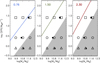 |
Fig. 2. Location in SFR stellar-mass diagram of the three galaxies selected as AGN hosts scaled to 1012 Lv, ⊙ (log(M⋆/M⊙)∼11.8), 1011 Lv, ⊙ (log(M⋆/M⊙)∼10.8), and 1010 Lv, ⊙ (log(M⋆/M⊙)∼9.8) luminosities. Symbols indicate the distinct hosts: circles → NGC 809, triangles → PGC 055442, and squares → NGC 7119A. The filled symbols correspond to the actual location of the three nearby galaxies (see Table A.1). At each redshift (top left labels), the solid line traces the main sequence (SFRMS) fitted by Pearson et al. (2018) (see also Table 2). Objects in the grey region correspond to quenched host galaxies. |
To cover three different ranges of luminosity and stellar mass, the MUSE data cubes of the three galaxies were scaled to sample three absolute V-band luminosities (log(LV/LV, ⊙) = 10, 11, 12), corresponding to MV = −20.19, −22.69, −25.1911, and log(M⋆/M⊙) > 9.8, 10.8, 11.8 using the mass-luminosity ratio in Bell & de Jong (2001). Since the total absolute magnitude in the V-band was not available in Hyperleda12 (Makarov et al. 2014) for the three galaxies, we used the B magnitude (see Table A.1) and applied an average colour correction for their morphological types (B − V ∼ 0.88, Mannucci et al. 2001) to estimate the V-band magnitudes. These scaled galaxies are representative of the population of host galaxies of type 1 AGNs at least up to redshift 1 (Ishino et al. 2020). Their locations in the SFR stellar-mass diagram (see Fig. 2) indicate that nearly half of the mock targets would correspond to star-forming hosts and the other half to quenched galaxies.
Before using these galaxies to create the inputs for HSIM, we brought their data cubes to rest-frame wavelength using their systemic velocities (see Table A.1). In the case of NGC 7119A, we used the systemic velocity of the NGC 7119 system (i.e. 9666 km s−1 from Hyperleda).
3.2. The AGN
To simulate the emission of the central AGN, we used a theoretical QSO spectrum assuming a continuum modelled as a power law of the following form: Fλ = A × λα, with α = −1.72, and A is a constant (in arbitrary units at this step) related to the luminosity density (Neugebauer et al. 1987).
On top of this continuum, we included the brightest emission lines from Hβ to [S II]λ6717,6731 adopting Gaussian profiles for them. Using the catalogue of spectral properties of type 1 AGNs by Calderone et al. (2017)13 (version 1.2.0), we fixed the parameters of these Gaussians by taking the mean values for objects at z < 0.7. In practice, we assumed Gaussian widths of σ = 4.8 Å and σ = 44 Å (equivalent to a FWHM of ∼700, and ∼6360 km s−1 at Hβ rest-frame wavelength), for the narrow and broad components of the emission lines. We also considered equivalent widths of ∼7 and ∼58 Å for the narrow and broad component of Hβ, respectively, and ∼19 Å for [OIII]λ5007. From the same catalogue and redshift range, the median and brightest [O III] luminosities of AGNs are roughly 1042 and 1043 erg s−1, corresponding to bolometric luminosities of 1045.5 and 1046.5 erg s−1 (Heckman et al. 2004), respectively. Then, the resulting theoretical spectrum in arbitrary units was scaled to these two [O III] luminosities (see Fig. 3). According to the characteristic X-ray luminosity of AGNs (Aird et al. 2015) and the correlation between X-ray and [O III] luminosities for type 1 AGNs (Berton et al. 2015), these two synthetic spectra should be representative of type 1 AGNs at around cosmic noon.
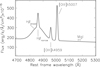 |
Fig. 3. Theoretical QSO spectrum scaled to L[OIII] = 1043 erg s−1 in the wavelength range of interest. Emission features in the range are labelled. For reference, we also marked the location of the MgI features indicative of the host’s stellar component. |
Using the simulated spectra and Eq. (1), we find that the faintest and brightest AGNs account for a black hole mass of ∼3.8 × 10⁸ M⊙, and ∼1.6 × 10⁹ M⊙, respectively. These MBH match the central black holes of galaxies around the cosmic noon according to observations (Kozłowski 2017) and the average growth history of SMBHs (Marconi et al. 2006). Taking into account the MBH stellar-mass relation (e.g. Eq. (9) from van den Bosch 2016) and assuming that is valid for any z, galaxies with stellar masses in the ∼1.3 − 4.6 × 10¹¹ M⊙ range should host black holes of that MBH at the redshifts of interest. Moreover, AGN luminosities appear related to the stellar mass and the SFR of their host galaxies. Taking into account the SFR of the selected hosts (see Sect. 3.1) and the AGN luminosities adopted in this work, our mock AGN+host would reside in evolutionary tracks closer to quenching (e.g. Mancuso et al. 2016). We note that a small fraction of quenched host galaxies at cosmic noon will host luminous AGNs (e.g. Florez et al. 2020).
3.3. Creating the input targets and running HSIM
The first step to create the input data cubes for HSIM was to build 11 rest-frame data cubes, two associated with the two simulated AGN spectra (see Sect. 3.2) and nine with the distinct luminosity-scaled host galaxies (see Sect. 3.1). The FoV of these data cubes were cropped to the size of the galaxies to save space and simulation computing time. Then, we added the AGN and host galaxy data cubes by placing the QSO at the nucleus of each host, limiting the spectral range to rest-wavelengths from 4770 to 5400 Å (i.e. Hβ-MgI region). We note that for the interacting system NG 7119, we placed the QSO at the centre of the northern galaxy (i.e. NGC 7119A; see Appendix A). All these data cubes were moved to three redshifts (z = 0.76, 1.50, and 2.30), applying the corresponding spatial resampling, spectral shifting, and brightness dimming. We fixed the spatial and spectral scales of these data cubes to 10 mas × 10 mas per spaxel and 2 Å per pixel, respectively, suiting the oversampling recommendations of HSIM but saving disk space. We note that to minimise effects when convolving the line-spread function and the PSF, HSIM internally performs spatial and spectral flux-conserving interpolations to the nominal scales for the selected setup (Zieleniewski et al. 2015). In summary, we obtained mock HARMONI observations for three redshifts, three host galaxy morphologies, three host galaxy luminosities, and two QSO bolometric luminosities, corresponding to 54 targets. In addition, we simulated 27 targets without an AGN (3 redshift × 3 morphologies × galaxy luminosities) and six targets with pure-QSO spectra (3 redshift × 2 QSO bolometric luminosities). These data cubes are the inputs for HSIM (HSIMInput hereafter).
Table 3 summarises the HSIM input parameters for the 87 generated targets. In all the cases, we fixed the total on-source observing time to 3 h, split into 12 exposures of 900 s each. We checked the dependency of the average S/N with the number of exposures (Nexp) for a fixed on-source integration time of 3 h, taking 3 × 3600 s as reference. We found an S/N percentage variation of ΔS/N(%)∼2.4 − 0.83 × Nexp and ΔS/N(%)∼1.4 − 0.49 × Nexp for IzJ and H + K gratings, respectively. Therefore, the mock HARMONI observations analysed in this work have a ∼7.5% in IzJ and ∼4.5% lower S/N than simulations performed splitting the 3 h of the total integration time in only three exposures of 3600 s each. Augustin et al. (2019) reported a 7% S/N gain when choosing 5 × 3600 s over 20 × 900 s for V + R grating. However, we note that in AO-assisted instruments, AO performances may vary during the exposure time. These variations result from changes in the atmospheric turbulence conditions and the airmass evolution (both functions of the wavelength). Thus, shorter individual exposures will be wiser to preserve the quality of the AO correction.
Summary of the input parameters to simulate HARMONI observations of AGNs and their host.
3.4. Flux calibration of the mock HARMONI observations
The HARMONI simulator (HSIM-version 300) can provide a flux-calibrated data cube. This requires the definition of a large enough aperture to determine the correction factors to translate detector counts into flux units with minimal flux uncertainties. However, we had to perform an independent flux calibration because the FoV of the HSIMInput data cubes was matched to the size of the host galaxies. We performed the flux calibration for IzJ and HK gratings after running HSIM and only in the spectral range corresponding to the Hβ+MgI region at redshifts 0.76, 1.50, and 2.30 (see Sect. 2.2). To calibrate the mock observations, one should mock observe a spectro-photometric standard star. Instead, as we applied HSIM to two point-like sources (QSOs of [OIII] luminosities 1042 and 1043 erg s−1) by each configuration, we used these data cubes to calibrate in flux. To do so, we integrated the flux using a circular aperture of 1.2 arcsec in radius to maximize the covered flux and S/N. We then compared the extracted spectra of each mock QSO observation at each luminosity and spectral range with the corresponding flux-calibrated spectra obtained from the input target. Such comparison provides the following linear calibration functions with lambda (see also Fig. 4) in the fitted spectral ranges:
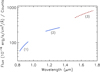 |
Fig. 4. Flux-density-to-counts ratio for the gratings (IzJ-blue and H + K-dashed red lines) used for the mock HARMONI observations of AGNs+hosts. We note that the derived functions only cover the Hβ+MgI spectral range (4770−5400 Å rest-frame wavelengths) at redshifts 0.76 (1), 1.50 (2), and 2.30 (3) due to the design of our simulations. |
fIzJ(λ) = (−3.19 + 4.55λ) × 10−18, if λ < 0.94 μm,
fIzJ(λ) = (−1.60 + 3.21λ) × 10−18, if 1.15 < λ < 1.33 μm,
fHK(λ) = (−1.51 + 1.33λ) × 10−19, if 1.54 < λ < 1.73 μm.
Finally, we applied these functions to each spaxel in our mock HARMONI observations to transform counts into flux. Comparing the resulting data cubes for the mock HARMONI pure AGNs with their corresponding HSIM inputs, we found uncertainties in the flux calibration that range between 1% and 5%.
4. Analysis and discussion of results
Through this section, we briefly describe the steps and methodology to analyse our mock HARMONI observations. We note that our simulations are constrained to the size of the objects (see Sect. 3.3), but the actual FoV of the HARMONI 20 × 20 mas2 scale is wider (see Table 1). For the analysis, we employed popular tools frequently used to analyse data of nearby galaxies. In this section, we only include the figures resulting from the analysis of the lenticular host (i.e. NGC 809). Appendix B shows the same figures for the spiral and interacting galaxies.
4.1. Band-filter images and host galaxy parameters
Adaptive optics systems greatly compensate for the atmospheric turbulence impact on data observed at ground-based telescopes. However, the resulting PSFs are complex, showing temporal and spatial variations in addition to their intrinsic wavelength dependence. Furthermore, turbulence residuals will produce a halo around the PSF peak; the worse the quality of the AO correction, the wider that PSF halo. Figure 5 shows images of the PSF for our mock HARMONI observations at three wavelength bands. The sizes of these complex PSFs are comparable to the angular size of the host galaxies at around cosmic noon (∼1 arcsec at z ∼ 1.5). Then, the actual AGN light spread halo may be brighter than the surface brightness of the host, especially in the higher contrast cases (see Fig. 5). Hence, the bright AGN light spreads all over, outshining the host and resulting in a blend of host and AGN spectra across the whole extent of the host galaxy (see Figs. 6 and 7). Thus, to study the underlying galaxies of distant AGNs, it is necessary to subtract the AGN contribution.
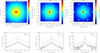 |
Fig. 5. PSF for HARMONI in the instrument configuration summaries in Table 3 at three wavelengths ranges. Upper panels: filter-band images (0.89−0.92 μm (left), 1.26−1.31 μm (centre), and 1.67−1.73 μm (right)). The 20 × 20 mas2 scale of our mock HARMONI observations undersamples the potential FWHM of the PSF, which varies from ∼6 mas at the bluest filter to ∼11 mas at the reddest one. Intensities are in logarithmic scale and normalised to the peak in each case. Lower panels: radial profiles along the right ascension axis and through the centre obtained from the filter-band image of the lenticular host galaxy scaled to 1011 Lv, ⊙ without QSO (black profile), the QSO of L[OIII] = 1042 (red dashed-profile), and the QSO of L[OIII] = 1043 (blue dotted-line). Intensities are normalised to the peak of the host in each case. |
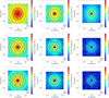 |
Fig. 6. Filter-band images obtained by integrating the signal of the HSIM output cubes in the spectral bands (Hβ+MgI region) of the IzJ-grating (0.82−0.93 μm (left) and 1.17−1.33 μm (centre)) and the H + K-grating (1.55−1.75 μm (right)) when considering a QSO of L[OIII] ∼ 1042 erg s−1 at the nucleus of the lenticular host (i.e. NGC 809) at redshifts 0.76 (left), 1.50 (middle), and 2.30 (right). Host luminosities are scaled to 1012 Lv, ⊙ (top), 1011 Lv, ⊙ (middle) and 1010 Lv, ⊙ (bottom). Intensity is in logarithmic scale and normalised to the peak of the brightest case (top left panel). Contours correspond to the average S/N in the rest-frame 5050−5250 Å corresponding to a stellar continuum region including the MgI features (brown contours are S/Ns of 0.06, 0.1, 0.3, and 0.6; S/Ns values of 2, 5, 9, 14, and 20 are drawn as blue contours; the purple contour indicates an S/Ns of 1). |
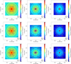 |
Fig. 7. Same as Fig. 6, but considering a QSO of L[OIII] ∼ 1043 erg s−1 at the nucleus of the lenticular host (i.e. NGC 809). |
Some specific tools have been developed to de-blend (on 2D or 3D data) the emission from the AGN and its host galaxy (see e.g. García-Lorenzo et al. 2005; Vayner et al. 2016; Husemann et al. 2016; Rupke et al. 2017; Varisco et al. 2018). These algorithms generally require a careful characterisation of the system PSF, which can be done following distinct reconstruction approaches (see e.g. Beltramo-Martin et al. 2020). That de-blending will inevitably introduce residuals that impact the S/N of the host spectrum and images. Procedures to optimally de-blend the AGN spectrum and the host galaxy data cube are beyond the scope of this paper and will be the focus of a forthcoming work considering distinct AO performances. In the meantime, we assume an optimal removal of the light from the central AGN, and we focus hereafter on the analysis of the mock HARMONI observations of the host galaxies only, without AGNs. This represents the ideal case of a perfect de-blending of the host and the central AGN light while simultaneously assessing the detection of non-active galaxies. However, even in this case, the shot noise introduced by the AGN light will always be added in quadrature to the detector noise sources, limiting the actual S/N. Detector systematics were not considered in our simulations (see Table 3). Nevertheless, we include some basic estimations to obtain an overview of the de-blending impact.
Hence, we integrated the mock HARMONI observations of the galaxies without AGN in the full spectral range of the corresponding gratings to obtain band-filter images. Figure 8 shows these images for the luminosity-scaled lenticular host morphology at the different redshifts. These images indicate a marginal detection (2-sigma ≤ signal ≤ 4-sigma) of the galaxies for the lowest host luminosity at z > 0.76. As a reference for redshift dimming, Table 4 includes the average S/N estimated within an aperture of 60 mas in radius centred on the nucleus of the hosts scaled to 1011 Lv, ⊙. We used the elliptical isophote analysis within the photutils Astropy package14 to estimate the photometric position angle (PAp) and the ellipticity (ϵ) from these recovered images (see Table 5). We were not able to perform good fits for the faintest cases. We found a good agreement (within uncertainties) in the position angles obtained for the HSIMInput and HSIM outputs (see Table 5). Ellipticities present some deviations, especially in the case of the interacting host. Deviations are larger when comparing with the actual photometric parameters of the three nearby galaxies (see Table A.1). The impact of spatial resolution on defining the morphological structures in the redshifted galaxies is the foremost driver of these deviations (see e.g. Mast et al. 2014).
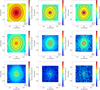 |
Fig. 8. Full-band images obtained by integrating the signal of the HSIM output cubes in the spectral band of the IzJ (left and central; 0.81−1.34 μm) and the H + K (right; 1.45−2.40 μm) gratings when considering the lenticular host (i.e. NGC 809) as a galaxy at redshifts 0.76 (left), 1.50 (middle), and 2.30 (right) scaled to 1012 Lv, ⊙ (top), 1011 Lv, ⊙ (middle), and 1010 Lv, ⊙ (bottom) as also labelled in each panel. Intensity is in logarithmic scale and normalised to the peak of the brightest case (top left panel). As in Figs. 6 and 7, contours correspond to the average S/N in the rest-frame 5050−5250 Å (black contours are S/Ns of 0.06, 0.1, 0.3, and 0.6; S/N values of 2, 5, 9, 14, and 20 are drawn as blue contours; the purple contour indicates an S/N of 1). |
Estimated effective radius at different redshifts of the galaxies acting as AGN hosts in the mock HARMONI simulations.
Based on filter-band images, Jahnke et al. (2009) established the detection limit for faint underlying host galaxies to be ∼3% of the total flux of the AGN in a defined aperture. To assess the potential impact of AGN subtraction on our results, we assume that particular 3% of the AGN flux as the host detection limit. Using the narrow-band flux-calibrated data cubes for the AGN and the host galaxies separately, we note that host galaxies are brighter than 3% of the AGN fluxes at the selected radii to estimate the photometric parameters. Only the hosts scaled to 1010 Lv, ⊙ combined with the brightest AGN (i.e. L[OIII] = 1043 erg s−1) host fluxes are under that threshold. Thus, the AGN removal will impact the estimation of the photometric parameters mainly in the highest contrast AGNs with faint hosts.
4.2. Integrated spectra of the hosts
For the mock HARMONI observations of the hosts, we obtained the integrated spectra by adding the signal of the spaxels within an aperture of twice the effective radius (Reff) in diameter. We estimate the radius of these apertures at each z (see Table 4) by applying the following:
![$$ \begin{aligned} R_{\rm eff}(z) = \left[\frac{1 + z}{1 + z_0}\right]^{\beta _{z}} R_{\rm eff}(z_0), \end{aligned} $$](/articles/aa/full_html/2022/03/aa41400-21/aa41400-21-eq7.gif)
where βz provides the rate of average size evolution of galaxies as a function of mass and galaxy type (see Table 2 in van der Wel et al. 2014). The adopted values for βz in each case are listed in Table 4. Table A.1 includes Reff(z0) for the three galaxies selected as hosts. For comparison, we also extracted the integrated spectra within the same apertures from the corresponding HSIMInput data cubes. Figure 9 shows these aperture-integrated spectra (see also Figs. B.4 and B.9).
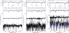 |
Fig. 9. Representative spectra of lenticular host (i.e. NGC 809) at redshifts 0.76 (left), 1.50 (centre), and 2.30 (right) obtained by adding the signal from the spaxels within the effective radius (see Table 4). Top panels: spectra extracted from the HSIMInputs, only for the host galaxy scaled to 1011 Lv, ⊙. Bottom panels: spectra from the mock HARMONI observation, after reduction and flux calibration, for the three host luminosities. The blue dotted lines correspond to the PPXF best-fit model for each spectrum. |
We estimated the S/N of these aperture-integrated spectra in the 5100−5230 Å rest wavelength corresponding to the MgI region (see Table 6). To do so, we obtained the best-fit model for the stellar continuum in the 4650−5250 Å rest-frame range using the penalised pixel-fitting (PPXF15) method (Cappellari & Emsellem 2004; Cappellari 2017) masking the emission lines. As templates, we used spectra from the ELODIE stellar library (Prugniel & Soubiran 2001) at R = 10 000. This is adequate for the instrumental resolution of the mock HARMONI data adjusted to the rest-frame Hβ–MgI range for the three redshifts considered. Similar results are obtained using the MILES stellar library as templates at z = 0.76 (Vazdekis et al. 2015). Figure 9 includes the best-fit models overplotted on the spectra (see also Figs. B.4 and B.9). The standard deviation of the residuals (spectrum – best-fit) provides an assessment of the noise in the MgI spectral range, to finally compute the S/N. PPXF also provides the stellar velocity and velocity dispersion of the spectrum under analysis (Table 6). PPXF only provides reliable estimations of the stellar kinematics for spectra with moderate-to-high S/N (e.g. S/N > 8 per spectral bin) (Cappellari & Emsellem 2004). The S/N of the integrated spectra for the faintest hosts are under this S/N threshold. As we shifted the spectra to the rest-frame wavelengths before running PPXF, the stellar velocities are around 0. The estimation of the stellar velocity dispersion from the aperture-integrated spectra with S/N > 8 for the mock HARMONI observations over the considered z range is in good agreement with the ones estimated for the HSIMInput, with uncertainties < 20%. Only in the case of the interacting host at the largest z, the uncertainty in σ⋆ is larger, reaching 40% (see Fig. 10).
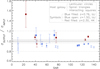 |
Fig. 10. Stellar velocity dispersion of aperture spectra obtained from the mock HARMONI observations relative to the stellar velocity dispersion of the HSIMInputs. Different symbols indicate the distinct hosts: circles → NGC 809, triangles → PGC 055442, and squares → NGC 7119A. Colours correspond to redshift and grating: blue filled symbols → z = 0.76, and IzJ grating; blue open symbols → z = 1.50, and IzJ grating; red filled symbols → z = 2.30, and HK grating. Grey dashed line marks the 20% level of uncertainty. Black dotted line indicates the typical uncertainty of σ⋆ for the HSIMInputs. Black solid line indicates σOUTPUT = σINPUT. |
Stellar velocity dispersion measured from the mock HARMONI observations of representative host galaxies of AGNs at three redshifts around cosmic noon.
To approach the potential impact on these measurements of the residuals after the AGN-host de-blending, we also obtained the corresponding integrated spectra for the mock HARMONI AGN+host data and fitted the AGN contribution (see Sect. 4.4). We used the der_snr algorithm16 (Stoehr et al. 2008) to estimate the S/N in the MgI region on the residual spectra after subtracting the fitted AGN contribution. On average, we found that the S/N is ∼18% (∼50%) lower than the S/Ns in Table 6 when the host luminosity is 1011 L⊙ (1010 L⊙). For the brightest hosts, the differences are comparable (∼1%) to the differences between the S/Ns in Table 6 and those estimated using der_snr (< 1%) on the host’s integrated spectra.
4.3. Resolved stellar kinematics
To spatially resolve the stellar kinematics, we only selected those spaxels within the outermost isophote with S/N ≥ 1, and spatially binned the spectra to achieve an S/N of about 8. This level provides reliable values of the first two moments of the line-of-sight velocity distribution (see Sect. 4.2), and it still preserves spatial resolution in the brightest mock HARMONI observations. Using the GIST17 pipeline (Bittner et al. 2019), we applied the Voronoi binning procedure described in Cappellari & Copin (2003) to ensure this S/N, and the PPXF code to derive the velocity and the velocity dispersion of each Voronoi-bin spectrum. We note that the actual spatial resolution of stellar kinematic maps will depend on the S/N threshold applied and the sizes of the resulting Voronoi-bins, smoothing the potential spatial resolution of the selected HARMONI scale. Figure 11 shows the derived stellar velocity fields and distribution of stellar velocity dispersions for the AGN-lenticular host (see Figs. B.5 and B.10 for the spiral and interacting hosts). The noisy appearance of the stellar kinematics maps is larger when increasing the redshift and decreasing the host luminosity. Residuals resulting after the sky subtraction, mainly for the H + K spectral configuration, strongly impact the derived stellar kinematics. These residuals result from the interpolations inside HSIM to match the spatial and spectral sampling of the input datacube to the HSIM internal samplings used to generate the mock data cubes.
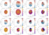 |
Fig. 11. Stellar kinematics of galaxies at redshifts around cosmic noon. Top panels: stellar velocity field (V⋆) and velocity dispersion distribution (σ⋆) obtained from mock HARMONI observations of three hours of on-source exposure time of lenticular (i.e. NGC 809) host galaxies scaled to the V-band luminosities indicated in each panel at redshifts 0.76 (a and b), 1.50 (c), and 2.30 (d), as also indicated. Bottom panels: same 2D-distributions but from mock HARMONI observations of six (e), nine (f and h), and 12 (g) hours of total exposure time of a lenticular hosts of the luminosities in the V band, which is labelled (i.e. 1011 L⊙ (e–g)) and 1010 L⊙ (h). Contours (in black) from the stellar continuum are overlaid in steps of 0.25 mag. For all panels, the colour bars are in the [−150,150] km s−1 and [20,200] km s−1 ranges for velocities and velocity dispersions, respectively. |
We fit the global kinematic position angle (PAk in Table 5) of these resolved stellar velocity fields using the PaFit18 code (Krajnović et al. 2006). In general, we found a good agreement between the position angles of the major kinematic axes derived for the HSIM inputs and HSIM outputs (Table 5). Large deviations result for poor, spatially resolved velocity fields (see Table 5). From the analysis of these simulations, we infer that three hours of total exposure with HARMONI are enough to resolve the stellar kinematics of the most massive hosts of AGNs at around cosmic noon.
We checked the dependency of the number of Voronoi bins at S/N ∼ 8 with exposure time to derive a reasonable observing limit to resolve the stellar kinematics of host galaxies with stellar masses in the M⋆ ∼ 1010 − 1011 M⊙ range. For that, we performed some additional simulations for the lenticular host (i.e. NGC 809) increasing the total exposure time to 6, 9, 12, or 15 h. Table 7 summarises the results in terms of number of voxels. Panels from e to h in Fig. 11 include the corresponding 2D distributions of velocities and velocity dispersions. Resolving the stellar velocity field of low-mass (i.e. M⋆ ≤ 1010 M⊙) galaxies beyond cosmic noon is an expensive challenge in terms of observing time, even for the ELT (> 15 h on-source per target). This estimation is in agreement with previous simulations for galaxies at 2 < z < 4 (Kendrew et al. 2016).
Number of Voronoi bins with S/N ≥ 8 in the 5100−5230 Å rest-wavelength resulting from mock HARMONI observations of the redshifted lenticular host (i.e. NGC 809) using 6, 9, 12, or 15 h (as indicated) on-source exposure times.
In the case of AGN hosts, the presence of the AGN poses an even bigger challenge. The stellar features will show a certain degree of dilution by the AGN continuum (e.g. Garcia-Rissmann et al. 2005). The AGN removal will impact the S/N of individual spaxels, probably limiting the spatial resolution and coverage of the stellar kinematics. However, the level of residuals might become small when combining spatial and spectral information, to the point that the relevant residuals would only affect the brightest 1 or 2 spaxels that trace the PSF (Husemann et al. 2016; Rupke et al. 2017). Moreover, gas outflows are ubiquitous in luminous AGNs, usually giving rise to double-peaked and multi-component emission-line profiles. The scale and orientation of these AGN-driven outflows might impact the determination of the stellar kinematics (see e.g. Gerssen et al. 2006). In particular, at the wavelength range of interest, the MgI features can be strongly contaminated by the complexity of the [NI]λ5199 emission line doublet resulting from the presence of multiple gaseous components (e.g. Fig. 5e in García-Lorenzo et al. 1999). For the considered QSO luminosities (i.e. L[O III] ∼ 1042, 1043 erg s−1), ionised outflows usually present velocities between 600 and 900 km s−1, and mass outflow rates in the range 1.5−50 M⊙ year−1 (e.g. Fiore et al. 2017). We do not include any feature accounting for such ionised outflows in our simulations. The wide range in the observed outflow properties makes it difficult to define a representative model.
4.4. Integrated spectra of the AGN+hosts: AGN parameters
Following the procedure described in Sect. 4.2, we also obtained the integrated spectra for the mock HARMONI observations of the AGN+hosts within an aperture of the Reff in radius. It is worth noting that the host galaxy contribution within these apertures is not negligible, resulting in a certain degree of dilution of the AGN features, mainly in the less contrasted cases. We performed a basic spectral analysis of these spectra in the 4725−5220 Å rest-frame spectral range using QSFIT13 (Calderone et al. 2017). We did not consider any iron contribution in the QSFIT modelling because it is not present in our AGN model (see Sect. 3.2). We note that QSFIT only includes a host galaxy for sources with z < 0.8. Figure 12 shows some examples of these integrated QSO+AGN spectra, including the QSFIT models overplotted. The QSFIT model uses Gaussian profiles to fit the broad and narrow components of the emission lines in the AGN+host spectra, providing their parameters. Figure 13 summarises the results for the different mock host’s AGN combinations. Differences between values for the input (dashed lines in Fig. 13) and the mock HARMONI pure AGNs (grey bands in Fig. 13) are negligible in all the brightest AGNs and many of the faintest AGN cases. Compared to the parameters of the pure AGN, only the faintest AGN shows large deviations when combined with the brightest host, and also the furthest cosmic distance. The design of the simulations, which includes an internal spectral interpolation (see Sect. 3), probably induces the non-negligible differences.
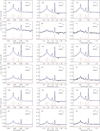 |
Fig. 12. Integrated spectra for the AGN+host (lenticular galaxy) at redshifts 0.76 (left), 1.50 (centre), and 2.30 (right) obtained by adding the signal from the spaxels within the host’s effective radius (see Sect. 4.2). The labels in the top right corner indicate the host and AGN (AGN42 → 1042 and AGN43 → 1043 erg s−1) luminosities. The numbers in the top left corners indicate the S/N in the rest-frame 5050−5250 Å obtained using the der_snr algorithm. The blue-dotted lines correspond to the QSFIT model to each spectrum. Red lines draw the Gaussian profiles fitting the broad (dotted line) and narrow (dashed line) components of the emission lines in the AGN spectra. |
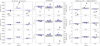 |
Fig. 13. Full width at half maximum of the broad Hβ (left panels) and narrow [OIII]λ5007 (central panels) components of the Gaussian profiles modelling the emission lines in the AGN+hosts’ integrated-spectra at the different redshifts (see text). Right panel: equivalent-width ratio of the broad and narrow components. Different symbols indicate the distinct hosts (circles → NGC 809, triangles → PGC 055442, and squares → NGC 7119A), and their colours indicate the [OIII] luminosities of the AGN (black filled symbols → 1042, and blue open symbols → 1043 erg s−1). Error bars correspond to the uncertainties provided by the QSFIT13 package if larger than the symbol size. Dashed lines are the adopted values to simulate the emission of the central AGN (see Sect. 3.2). Grey bands indicate the parameters obtained when fitting the integrated spectra obtained from the mock HARMONI data for the pure AGN, enclosing the values and uncertainties for the two AGN luminosities. |
5. Summary and conclusions
The new generation of 30−40-m class telescopes will be a major revolution for astrophysics, opening new frontiers. As a first light instrument for the ELT, HARMONI will be a very versatile integral field spectrograph supporting a broad range of science programmes. Given the multiple instrument settings (e.g. spaxel scale, gratings, AO mode, etc.), it is valuable to quantify in advance the expected performances for specific science cases.
Focusing on the context of the co-evolution of galaxies and their central black holes, we explored the potential of HARMONI to resolve the morpho-kinematics of the host galaxy of AGNs at redshifts around cosmic noon. We used the dedicated simulation pipeline HSIM (version 300) to perform a set of mock HARMONI observations for the 20 × 20 mas2 spatial scale, a spectral resolution of R = 3200, and LTAO working at 0.67 arcsec seeing. To create the input targets for HSIM, we generated synthetic AGN spectra and took advantage of available IFS data of nearby galaxies with distinct morpho-kinematics. We scaled these two ingredients to different AGN and host galaxy luminosities, combined them, and artificially dimmed and redshifted them to the chosen cosmic epoch. Our main results and conclusions are summarised as follows:
-
The two coarser scales of HARMONI seem to be the best suited to reveal the host galaxies of distant AGNs. Their FoVs extend beyond the average size of the host galaxies, including the expected size of the outflows, and simultaneously observing the sky background.
-
The low-resolution gratings of HARMONI provide the opportunity to resolve the stellar kinematics of galaxies using a homogeneous procedure from before cosmic noon to the local Universe, with similar velocity resolution to IFS legacy surveys of nearby and intermediate-redshift galaxies.
-
In three hours of on-source integration, HARMONI low-spectral resolution observations with the 20 × 20 mas2 spatial scale will reveal the morphology of galaxies brighter than 1010 L⊙ around cosmic noon, allowing the estimation of basic morphological parameters (type, position angles, or inclination). These observations will also provide reliable estimations of their stellar velocity and velocity dispersions at the effective radius with S/Ns over 8 in the stellar continuum.
-
ELT+HARMONI will resolve the stellar kinematics of massive galaxies (M⋆ ≥ 1011 M⊙) up to and beyond cosmic noon when observing under median atmospheric conditions for three hours.
-
HARMONI observations including the ones mock here will allow reliable measurements of the emission line parameters of the central AGN for almost all the considered cases. Only those with the lowest AGN-host contrasts show discrepancies not attributable to the design of the simulations.
-
The simulations described here show that from the ELT+HARMONI observations we can simultaneously measure the MBH and the resolved stellar kinematics of galaxies (M⋆ > 1010.5 M⊙) hosting bright AGN at a redshift around cosmic noon using total exposure times that can vary from three to 15 h.
As we already discussed, a major challenge to reveal the morpho-kinematics of distant AGN hosts is the de-blending the AGN and host galaxy spectra with negligible residuals. The reconstruction of the complex and variable PSF in IFS data is key to this goal. The next step of this work is to explore the reliability of 3D-PSF reconstruction for AO-assisted IFS observations.
V⊙ = +4.81 (Willmer 2018).
Acknowledgments
We are grateful to Laura Sánchez-Menguiano for kindly sharing the (10), (11), (12), and (13) entries in Table A.1 for NGC 809. We also thank Michele Cappellari, Ignacio Ferreras and Ignacio Martín-Navarro for their useful comments. B.G.-L. and A.M.-I. acknowledge support from the Spanish Ministry of Science, Innovation and Universities (MCIU), Agencia Estatal de Investigación (AEI), and the Fondo Europeo de Desarrollo Regional (EU-FEDER) under projects with references AYA2015-68217-P and PID2019-107010GB-100. B.G.-L., A.M.-I., C.R.A. and E.M.G. also acknowledge financial support from the State Agency for Research of the Spanish MCIU through the Center of Excellence Severo Ochoa award to the Instituto de Astrofísica de Canarias (SEV-2015-0548 and CEX2019-000920-S). M.P.S. acknowledges support from the Comunidad de Madrid through the Atracción de Talento Investigador Grant 2018-T1/TIC-11035 and PID2019-105423GA-I00 (MCIU/AEI/EU-FEDER). N.T. acknowledges support from the Science and Technology Facilities Council (grant ST/N002717/1), as part of the UK E-ELT Programme at the University of Oxford. C.R.A. acknowledges financial support from the Spanish MCIU under grant with reference RYC-2014-15779, from the European Union’s Horizon 2020 research and innovation programme under Marie Skłodowska-Curie grant agreement No. 860744 (BiD4BESt), from the State Research Agency (AEI-MCINN) of the Spanish MCIU under grants PID2019-106027GBC42 and EUR2020-112266. C.R.A. also acknowledges support from the Consejería de Economía, Conocimiento y Empleo del Gobierno de Canarias and the EU-FEDER under grant with reference ProID2020010105. L.G. acknowledges financial support from the Spanish Ministry of Science, Innovation and Universities (MCIU) under the 2019 Ramón y Cajal program RYC2019-027683 and from the Spanish MCIU project HOSTFLOWS PID2020-115253GA-I00. We also acknowledge the usage of the HyperLeda database (http://leda.univ-lyon1.fr). This research has made use of the SIMBAD database, operated at CSD, Strasbourg, France.
References
- Aird, J., Coil, A. L., Georgakakis, A., et al. 2015, MNRAS, 451, 1892 [Google Scholar]
- Arribas, S., Thatte, N. A., Tecza, M., et al. 2010, SPIE Conf. Ser., 7735, 77355H [NASA ADS] [Google Scholar]
- Augustin, R., Quiret, S., Milliard, B., et al. 2019, MNRAS, 489, 2417 [NASA ADS] [CrossRef] [Google Scholar]
- Bacon, R., Copin, Y., Monnet, G., et al. 2001, MNRAS, 326, 23 [Google Scholar]
- Baron, D., & Ménard, B. 2019, MNRAS, 487, 3404 [CrossRef] [Google Scholar]
- Bell, E. F., & de Jong, R. S. 2001, ApJ, 550, 212 [Google Scholar]
- Beltramo-Martin, O., Ragland, S., Fétick, R., et al. 2020, SPIE Conf. Ser., 11448, 114480A [NASA ADS] [Google Scholar]
- Berton, M., Foschini, L., Ciroi, S., et al. 2015, A&A, 578, A28 [NASA ADS] [CrossRef] [EDP Sciences] [Google Scholar]
- Bessiere, P. S., Tadhunter, C. N., Ramos Almeida, C., & Villar Martín, M. 2012, MNRAS, 426, 276 [NASA ADS] [CrossRef] [Google Scholar]
- Bittner, A., Falcón-Barroso, J., Nedelchev, B., et al. 2019, A&A, 628, A117 [NASA ADS] [CrossRef] [EDP Sciences] [Google Scholar]
- Brusa, M., Perna, M., Cresci, G., et al. 2016, A&A, 588, A58 [NASA ADS] [CrossRef] [EDP Sciences] [Google Scholar]
- Bundy, K., Bershady, M. A., Law, D. R., et al. 2015, ApJ, 798, 7 [Google Scholar]
- Calderone, G., Nicastro, L., Ghisellini, G., et al. 2017, MNRAS, 472, 4051 [Google Scholar]
- Cappellari, M. 2017, MNRAS, 466, 798 [Google Scholar]
- Cappellari, M., & Copin, Y. 2003, MNRAS, 342, 345 [Google Scholar]
- Cappellari, M., & Emsellem, E. 2004, PASP, 116, 138 [Google Scholar]
- Chiaberge, M., Gilli, R., Lotz, J. M., & Norman, C. 2015, ApJ, 806, 147 [NASA ADS] [CrossRef] [Google Scholar]
- Circosta, C., Mainieri, V., Padovani, P., et al. 2018, A&A, 620, A82 [EDP Sciences] [Google Scholar]
- Contini, T., Epinat, B., Bouché, N., et al. 2016, A&A, 591, A49 [NASA ADS] [CrossRef] [EDP Sciences] [Google Scholar]
- Croom, S. M., Lawrence, J. S., Bland-Hawthorn, J., et al. 2012, MNRAS, 421, 872 [NASA ADS] [Google Scholar]
- den Brok, M., Carollo, C. M., Erroz-Ferrer, S., et al. 2020, MNRAS, 491, 4089 [NASA ADS] [Google Scholar]
- Di Matteo, T., Springel, V., & Hernquist, L. 2005, Nature, 433, 604 [NASA ADS] [CrossRef] [Google Scholar]
- Donnari, M., Pillepich, A., Nelson, D., et al. 2019, MNRAS, 485, 4817 [Google Scholar]
- Esdaile, J., Glazebrook, K., Labbé, I., et al. 2021, ApJ, 908, L35 [NASA ADS] [CrossRef] [Google Scholar]
- Falcón-Barroso, J., Sánchez-Blázquez, P., Vazdekis, A., et al. 2011, A&A, 532, A95 [Google Scholar]
- Falcón-Barroso, J., Lyubenova, M., van de Ven, G., et al. 2017, A&A, 597, A48 [NASA ADS] [CrossRef] [EDP Sciences] [Google Scholar]
- Fiore, F., Feruglio, C., Shankar, F., et al. 2017, A&A, 601, A143 [NASA ADS] [CrossRef] [EDP Sciences] [Google Scholar]
- Florez, J., Jogee, S., Sherman, S., et al. 2020, MNRAS, 497, 3273 [NASA ADS] [CrossRef] [Google Scholar]
- Floyd, D. J. E., Kukula, M. J., Dunlop, J. S., et al. 2004, MNRAS, 355, 196 [NASA ADS] [CrossRef] [Google Scholar]
- Floyd, D. J. E., Dunlop, J. S., Kukula, M. J., et al. 2013, MNRAS, 429, 2 [NASA ADS] [CrossRef] [Google Scholar]
- Förster Schreiber, N. M., & Wuyts, S. 2020, ARA&A, 58, 661 [Google Scholar]
- Förster Schreiber, N. M., Renzini, A., Mancini, C., et al. 2018, ApJS, 238, 21 [Google Scholar]
- Fraser-McKelvie, A., Cortese, L., van de Sande, J., et al. 2021, MNRAS, 503, 4992 [NASA ADS] [CrossRef] [Google Scholar]
- Galbany, L., Anderson, J. P., Rosales-Ortega, F. F., et al. 2016, MNRAS, 455, 4087 [NASA ADS] [CrossRef] [Google Scholar]
- García-Benito, R., Zibetti, S., Sánchez, S. F., et al. 2015, A&A, 576, A135 [Google Scholar]
- García-Lorenzo, B., Mediavilla, E., & Arribas, S. 1999, ApJ, 518, 190 [CrossRef] [Google Scholar]
- García-Lorenzo, B., Sánchez, S. F., Mediavilla, E., González-Serrano, J. I., & Christensen, L. 2005, ApJ, 621, 146 [CrossRef] [Google Scholar]
- García-Lorenzo, B., Márquez, I., Barrera-Ballesteros, J. K., et al. 2015, A&A, 573, A59 [NASA ADS] [CrossRef] [EDP Sciences] [Google Scholar]
- García-Lorenzo, B., Monreal-Ibero, A., Mediavilla, E., Pereira-Santaella, M., & Thatte, N. 2019, Front. Astron. Space Sci., 6, 73 [CrossRef] [Google Scholar]
- Garcia-Rissmann, A., Vega, L. R., Asari, N. V., et al. 2005, MNRAS, 359, 765 [CrossRef] [Google Scholar]
- Gerssen, J., Allington-Smith, J., Miller, B. W., Turner, J. E. H., & Walker, A. 2006, MNRAS, 365, 29 [NASA ADS] [CrossRef] [Google Scholar]
- Graham, A. W. 2008, ApJ, 680, 143 [NASA ADS] [CrossRef] [Google Scholar]
- Guérou, A., Krajnović, D., Epinat, B., et al. 2017, A&A, 608, A5 [Google Scholar]
- Guyon, O., Sanders, D. B., & Stockton, A. N. 2006, New Astron. Rev., 50, 748 [Google Scholar]
- Harrison, C. M., Alexander, D. M., Swinbank, A. M., et al. 2012, MNRAS, 426, 1073 [NASA ADS] [CrossRef] [Google Scholar]
- Heckman, T. M., Kauffmann, G., Brinchmann, J., et al. 2004, ApJ, 613, 109 [Google Scholar]
- Husemann, B., Bennert, V. N., Scharwächter, J., Woo, J.-H., & Choudhury, O. S. 2016, MNRAS, 455, 1905 [NASA ADS] [CrossRef] [Google Scholar]
- Ishino, T., Matsuoka, Y., Koyama, S., et al. 2020, PASJ, 72, 83 [NASA ADS] [CrossRef] [Google Scholar]
- Jahnke, K., & Macciò, A. V. 2011, ApJ, 734, 92 [NASA ADS] [CrossRef] [Google Scholar]
- Jahnke, K., Elbaz, D., Pantin, E., et al. 2009, ApJ, 700, 1820 [NASA ADS] [CrossRef] [Google Scholar]
- Kaspi, S., Smith, P. S., Netzer, H., et al. 2000, ApJ, 533, 631 [Google Scholar]
- Kauffmann, G., Heckman, T. M., Tremonti, C., et al. 2003, MNRAS, 346, 1055 [Google Scholar]
- Kendrew, S., Zieleniewski, S., Houghton, R. C. W., et al. 2016, MNRAS, 458, 2405 [NASA ADS] [CrossRef] [Google Scholar]
- Kormendy, J., & Ho, L. C. 2013, ARA&A, 51, 511 [Google Scholar]
- Kozłowski, S. 2017, ApJS, 228, 9 [CrossRef] [Google Scholar]
- Krajnović, D., Cappellari, M., de Zeeuw, P. T., & Copin, Y. 2006, MNRAS, 366, 787 [Google Scholar]
- Law, D. R., Cherinka, B., Yan, R., et al. 2016, AJ, 152, 83 [Google Scholar]
- Leung, G. C. K., Coil, A. L., Aird, J., et al. 2019, ApJ, 886, 11 [NASA ADS] [CrossRef] [Google Scholar]
- Madau, P., & Dickinson, M. 2014, ARA&A, 52, 415 [Google Scholar]
- Mahoro, A., Pović, M., & Nkundabakura, P. 2017, MNRAS, 471, 3226 [Google Scholar]
- Makarov, D., Prugniel, P., Terekhova, N., Courtois, H., & Vauglin, I. 2014, A&A, 570, A13 [NASA ADS] [CrossRef] [EDP Sciences] [Google Scholar]
- Mancuso, C., Lapi, A., Shi, J., et al. 2016, ApJ, 833, 152 [NASA ADS] [CrossRef] [Google Scholar]
- Mannucci, F., Basile, F., Poggianti, B. M., et al. 2001, MNRAS, 326, 745 [Google Scholar]
- Marconi, A., Comastri, A., Gilli, R., et al. 2006, Mem. Soc. Astron. It., 77, 742 [NASA ADS] [Google Scholar]
- Marsden, C., Shankar, F., Ginolfi, M., & Zubovas, K. 2020, Front. Phys., 8, 61 [NASA ADS] [CrossRef] [Google Scholar]
- Marziani, P., & Sulentic, J. W. 2012, New Astron. Rev., 56, 49 [Google Scholar]
- Mast, D., Rosales-Ortega, F. F., Sánchez, S. F., et al. 2014, A&A, 561, A129 [NASA ADS] [CrossRef] [EDP Sciences] [Google Scholar]
- McLure, R. J., & Jarvis, M. J. 2002, MNRAS, 337, 109 [Google Scholar]
- Mendel, J. T., Beifiori, A., Saglia, R. P., et al. 2020, ApJ, 899, 87 [NASA ADS] [CrossRef] [Google Scholar]
- Naab, T., & Ostriker, J. P. 2017, ARA&A, 55, 59 [Google Scholar]
- Nesvadba, N. P. H., Lehnert, M. D., Eisenhauer, F., et al. 2006, ApJ, 650, 693 [NASA ADS] [CrossRef] [Google Scholar]
- Neugebauer, G., Green, R. F., Matthews, K., et al. 1987, ApJS, 63, 615 [NASA ADS] [CrossRef] [Google Scholar]
- Pearson, W. J., Wang, L., Hurley, P. D., et al. 2018, A&A, 615, A146 [NASA ADS] [CrossRef] [EDP Sciences] [Google Scholar]
- Pensabene, A., Carniani, S., Perna, M., et al. 2020, A&A, 637, A84 [NASA ADS] [CrossRef] [EDP Sciences] [Google Scholar]
- Peterson, B. M., Ferrarese, L., Gilbert, K. M., et al. 2004, ApJ, 613, 682 [Google Scholar]
- Planck Collaboration XIII. 2016, A&A, 594, A13 [NASA ADS] [CrossRef] [EDP Sciences] [Google Scholar]
- Proshina, I. S., Kniazev, A. Y., & Sil’chenko, O. K. 2019, AJ, 158, 5 [NASA ADS] [CrossRef] [Google Scholar]
- Prugniel, P., & Soubiran, C. 2001, A&A, 369, 1048 [CrossRef] [EDP Sciences] [Google Scholar]
- Ramón-Pérez, M., Bongiovanni, Á., Pérez García, A. M., et al. 2019, A&A, 631, A11 [Google Scholar]
- Ramos Almeida, C., Tadhunter, C. N., Inskip, K. J., et al. 2011, MNRAS, 410, 1550 [NASA ADS] [Google Scholar]
- Rizzo, F., Vegetti, S., Powell, D., et al. 2020, Nature, 584, 201 [Google Scholar]
- Rupke, D. S. N., Gültekin, K., & Veilleux, S. 2017, ApJ, 850, 40 [NASA ADS] [CrossRef] [Google Scholar]
- Saglia, R. P., Opitsch, M., Erwin, P., et al. 2016, ApJ, 818, 47 [Google Scholar]
- Sánchez, S. F. 2020, ARA&A, 58, 99 [Google Scholar]
- Sánchez, S. F., García-Benito, R., Zibetti, S., et al. 2016, A&A, 594, A36 [Google Scholar]
- Sánchez-Menguiano, L., Sánchez, S. F., Pérez, I., et al. 2018, A&A, 609, A119 [NASA ADS] [CrossRef] [EDP Sciences] [Google Scholar]
- Schreiber, C., Pannella, M., Elbaz, D., et al. 2015, A&A, 575, A74 [NASA ADS] [CrossRef] [EDP Sciences] [Google Scholar]
- Schreiber, N. M. F., Übler, H., Davies, R. L., et al. 2019, ApJ, 875, 21 [NASA ADS] [CrossRef] [Google Scholar]
- Shankar, F., Bernardi, M., Sheth, R. K., et al. 2016, MNRAS, 460, 3119 [NASA ADS] [CrossRef] [Google Scholar]
- Sharma, G., Salucci, P., Harrison, C. M., van de Ven, G., & Lapi, A. 2021, MNRAS, 503, 1753 [CrossRef] [Google Scholar]
- Shen, Y. 2013, Bull. Astron. Soc. India, 41, 61 [NASA ADS] [Google Scholar]
- Shen, Y., Richards, G. T., Strauss, M. A., et al. 2011, ApJS, 194, 45 [Google Scholar]
- Silverman, J. D., Treu, T., Ding, X., et al. 2019, ApJ, 887, L5 [NASA ADS] [CrossRef] [Google Scholar]
- Skidmore, W., Els, S., Travouillon, T., et al. 2009, PASP, 121, 1151 [NASA ADS] [CrossRef] [Google Scholar]
- Smith, K. L., Koss, M., Mushotzky, R., et al. 2020, ApJ, 904, 83 [NASA ADS] [CrossRef] [Google Scholar]
- Stark, D. V., Bundy, K. A., Westfall, K., et al. 2018, MNRAS, 480, 2217 [NASA ADS] [CrossRef] [Google Scholar]
- Stoehr, F., White, R., Smith, M., et al. 2008, in Astronomical Data Analysis Software and Systems XVII, eds. R. W. Argyle, P. S. Bunclark, & J. R. Lewis, ASP Conf. Ser., 394, 505 [NASA ADS] [Google Scholar]
- Thatte, N. A., Clarke, F., Bryson, I., et al. 2016, SPIE Conf. Ser., 9908, 99081X [NASA ADS] [Google Scholar]
- Thatte, N. A., Bryson, I., Clarke, F., et al. 2020, SPIE Conf. Ser., 11447, 114471W [NASA ADS] [Google Scholar]
- Thomas, D., Steele, O., Maraston, C., et al. 2013, MNRAS, 431, 1383 [NASA ADS] [CrossRef] [Google Scholar]
- Treister, E., Schawinski, K., Urry, C. M., & Simmons, B. D. 2012, ApJ, 758, L39 [NASA ADS] [CrossRef] [Google Scholar]
- van den Bosch, R. C. E. 2016, ApJ, 831, 134 [NASA ADS] [CrossRef] [Google Scholar]
- van der Wel, A., Franx, M., van Dokkum, P. G., et al. 2014, ApJ, 788, 28 [Google Scholar]
- van der Wel, A., Bezanson, R., D’Eugenio, F., et al. 2021, ApJS, 256, 44 [NASA ADS] [CrossRef] [Google Scholar]
- van de Sande, J., Bland-Hawthorn, J., Brough, S., et al. 2017, MNRAS, 472, 1272 [NASA ADS] [CrossRef] [Google Scholar]
- Varisco, L., Sbarrato, T., Calderone, G., & Dotti, M. 2018, A&A, 618, A127 [NASA ADS] [CrossRef] [EDP Sciences] [Google Scholar]
- Vayner, A., Wright, S. A., Do, T., et al. 2016, ApJ, 821, 64 [NASA ADS] [CrossRef] [Google Scholar]
- Vayner, A., Wright, S. A., Murray, N., et al. 2017, ApJ, 851, 126 [Google Scholar]
- Vazdekis, A., Coelho, P., Cassisi, S., et al. 2015, MNRAS, 449, 1177 [Google Scholar]
- Vestergaard, M., & Peterson, B. M. 2006, ApJ, 641, 689 [Google Scholar]
- Willmer, C. N. A. 2018, ApJS, 236, 47 [Google Scholar]
- Wisnioski, E., Förster Schreiber, N. M., Wuyts, S., et al. 2015, ApJ, 799, 209 [Google Scholar]
- Wright, E. L. 2006, PASP, 118, 1711 [NASA ADS] [CrossRef] [Google Scholar]
- Zakamska, N. L., Sun, A.-L., Strauss, M. A., et al. 2019, MNRAS, 489, 497 [Google Scholar]
- Zieleniewski, S., Thatte, N., Kendrew, S., et al. 2015, MNRAS, 453, 3754 [Google Scholar]
Appendix A: Individual galaxies
In this work, we selected three galaxies observed in the AMUSING survey (Galbany et al. 2016) as prototypes for the host galaxies of AGNs at the desired cosmic epoch (see Sect. 3.1). This appendix is focused on showing the main characteristics of these galaxies. Table A.1 presents the basic data for them. Details on the data processing are provided in Galbany et al. (2016).
Basic parameters of the three nearby objects selected as models for the host galaxies of AGN at redshifts around the cosmic noon (see Sect. 3.1).
For each object, we obtained a ‘total’ spectrum (see Fig. A.1) by adding up the spectra of all spaxels in the MUSE data cubes (see Sect. 3.1) inside a projected circular aperture of a diameter equal to the Reff. We estimated the systemic velocity and stellar velocity dispersion (see Table A.1) applying the PPXF code (Cappellari & Emsellem 2004; Cappellari 2017) on these spectra in the rest-frame 4800-5300 Å wavelength range, with the emission-lines masked. We also present here the stellar velocity fields and velocity dispersion maps extracted from the MUSE data cubes. We measured the stellar kinematics using PPXF through the GIST pipeline (Bittner et al. 2019). We applied the Voronoi binning scheme of Cappellari & Copin (2003) to spatially bin the data to homogenise the S/N of the analysed spectra to ∼8 in this spectral range. The spaxels with an estimated S/N below 1 were discarded. These S/N thresholds are the same as those selected for the AGN hosts at different redshifts. We used the MILES model library as a template (Vazdekis et al. 2015) at a spectral resolution of 2.51 Å (Falcón-Barroso et al. 2011). The MILES library provides the smallest difference between the spectral resolution of the stellar templates and the MUSE instrument resolution (∼2.85 Å at 0.5 μm, Guérou et al. 2017). Figures A.2, A.3, and A.4 show the stellar velocity and velocity dispersion maps for NGC 809, PGC 055442, and NGC 7119, respectively.
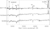 |
Fig. A.1. Total spectra of the three nearby galaxies picked as host for our simulations of AGN+host observations with HARMONI. Spectra were normalised to the average intensity in the plotted wavelength range. The horizontal axis corresponds to rest-frame wavelengths. The spectra are shown in logarithmic scale and arbitrarily shifted on the vertical axis. Dashed-vertical lines indicate the spectral range included in the HARMONI simulations. Labels mark the position of several emission (i.e. Hβ, [O III]λ5007, HeIλ5876, [NII]λ6543, Hα, and [NII]λ6584) and absorption lines (i.e. MgIλ5163, 5172, 5183, FeIλ5269, and NaIλ5889, 5895). Dotted rectangle indicates the zoomed-in image of a region in Fig. A.5 for the NGC 7119A spectrum. |
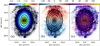 |
Fig. A.2. (a) Filter-band image of NGC 809 obtained by collapsing the MUSE data cube over the rest-frame spectral range 5100-5230 Å. (b) NGC 809 line-of-sight stellar velocity field. (c) Stellar velocity dispersion map of NGC 809. We plot all the MUSE spaxels with S/N> 1 in the 5100-5230 Å rest-frame. Limits of the colour bar are [-150,150] km s−1 and [20,200] km s−1 for velocity (panel (b)) and velocity dispersion (panel (c)), respectively. These are the same limits as those selected for the AGN hosts in Fig. 11. Contours (in black) correspond to the stellar continuum in steps of 0.25 mag. |
A.1. NGC 809
NGC 809 is a lenticular galaxy showing two bright UV and optical rings at ∼3.5 kpc (∼10 arcsec) and ∼9 kpc (25.5 arcsec) in which star formation activity has ceased (Proshina et al. 2019). The integrated spectrum of NGC 809 (see Fig. A.1) is dominated by the stellar continuum in the 4800-6600 Å spectral range. Emission line features are not evident in this range and only [NII]λ6584 can be visually identified. The stellar velocity field of NGC 809 presents a clear rotation pattern, with the kinematic major axis well-aligned with the photometric position angle (Table A.1). The peak-to-peak amplitude of the velocity field is ∼267 km s−1 and the kinematic centre is in agreement with the optical nucleus position (coordinate origin in panels of Fig. A.1). The global kinematic position angle (PAk) is −7 ± 3 degrees. The stellar velocity dispersion peaks (∼160 km s−1) at the optical nucleus decreasing outwards.
A.2. PGC 055442
PGC 055442 is an early-type barred spiral galaxy at redshift ∼0.02358. It is morphologically mis-classified as an elliptical galaxy by HyperLeda12, which is evident from the spiral structure in the Hα-filter images recovered from MUSE data (see Fig. D1 in Sánchez-Menguiano et al. 2018). The spectrum of PGC 055442 (see Fig. A.1) is dominated by the stellar continuum, although [NII]λ6548, Hα, and [NII]λ6584 emission lines are clearly identified. The Hβ absorption feature is not evident because of an emission peak at its position. A weak [O III]λ5007 emission line also seems to be present. The filter-band image in Fig. A.3 shows the existence of a stellar bar along a position angle of about 45 degrees, offset by ∼30 degrees from the large-scale photometric axis (Table A.1). The stellar velocity field is consistent with a regular rotational pattern, with the major kinematic angle (PAk = 12 ± 3 degrees) aligned with the photometric axis (Table A.1) and a projected velocity amplitude (peak-to-peak) of ∼360 km s−1. The stellar velocity dispersion shows relatively high values at the central region, with the peak (∼148 km s−1) at the optical nucleus and dropping off to an almost constant velocity dispersion of about 55 km s−1 from 7 arcsec.
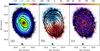 |
Fig. A.3. Same as Fig. A.2, but for PGC 055442. Limits of the colour bar are [-180,180] km s−1 and [20,200] km s−1 for velocity (panel (b)) and velocity dispersion (panel (c)), respectively. These are the same limits as those selected for the AGN hosts in Fig. B.5. |
A.3. NGC 7119A
NGC 7119A is a barred spiral galaxy in an initial stage of interaction with its close companion NGC 7119B. The systemic velocity of the system (NGC 7119A and NGC 7119B) is 9666 km s−1 (from HyperLeda12). The NGC 7119B centre is located about 12 arcsec to the southeast of the NGC 7119A nucleus, with a systemic velocity difference of ΔV ∼ −283 km s−1 and a difference of ∼0.31 magnitudes in total B magnitude (from HyperLeda12). The integrated spectrum of NGC 7119A resembles those typical of spiral galaxies, displaying pronounced absorption features, bright [NII]λλ6548, 6584 and Balmer emission lines and faint [O III]λλ4959, 5007 lines. However, it shows the presence of double peaks in the emission line profiles as result of two kinematically distinct components. The reddest component is associated with the ionised gas in NGC 7119A. The second component, at about 280 km s−1 blueshifted, is placed at the corresponding wavelength position for the ionised gas in its close companion, NGC 7119B. Figure A.5 zooms in on the wavelength range between 6520 and 6610 Å, including only the [NII]λ6548, Hα and [NII]λ6584 emission lines to clearly show these double-peaked profiles. The blending with NGC 7119B light is unclear from the stellar absorption lines in the NGC 7119A spectrum. The filter-band image (see Fig. A.4-left) clearly shows the spiral morphology of NGC 7119A. Although its companion NGC 7119B is in front of it, the continuum emission seems to be dominated by NGC 7119A in the light-of-sight overlap region, where the prominent southeastern spiral arm of NGC 7119A is located. The stellar velocity field of NGC 7119A resembles a typical rotation supported spiral galaxy, with the photometric (Table A.1) and major kinematic axes (PAk = −35 ± 3) aligned. However, it is distorted in the southeast due to the overlap with the NGC 7119B stellar kinematics. The peak-to-peak velocity amplitude along the major kinematic axis is ∼386 km s−1. The stellar velocity dispersion map reaches values over 400 km s−1 in the overlapping region of NGC 7119 system. The stellar velocity dispersion at the optical nucleus of NGC 7119A is ∼116 km s−1. There is a region with average velocity dispersion of ∼330 km s−1 at about four arcsec southeast of the NGC 7119A nucleus extending to the east and west by about 1.5 arcsec. These high values of the velocity dispersion are most probably associated with a superposed contribution of the stellar components from NGC 7119B along the lines of sight of NGC 7119A, which is not evident in the stellar features of the integrated spectrum, but is evident in the emission lines (see Fig. A.5).
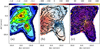 |
Fig. A.4. Same as Fig. A.2, but for NGC 7119A. Limits of the colour bar are [-350,350] km s−1 and [20,350] km s−1 for velocity (panel (b)) and velocity dispersion (panel (c)), respectively. These are the same limits as those selected for the AGN hosts in Fig. B.10. |
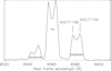 |
Fig. A.5. Hα+[NII]λλ6548, 6584 emission line profiles observed in the integrated spectrum of NGC 7119A. Double-peak profiles are the result of the contribution from its close companion, NGC 7119B. |
Appendix B: Fits
In this appendix, we include the intensity maps, the fits to the integrated spectra within the effective radius, and the resolved stellar kinematics for the spiral galaxy PGC 055442 and the interacting galaxy NGC 7119A simulating the host galaxies at redshifts 0.76, 1.50, and 2.30.
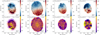 |
Fig. B.5. Same as Fig. 11 (top-panels), but for a spiral host galaxy (i.e. PGC 0055442). Colour bars are in the [-180,180] km s−1 and [20,200] km s−1 ranges for velocities and velocity dispersions, respectively. |
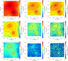 |
Fig. B.8. Same as Fig. 8, but when considering the interacting morphology (i.e. NGC 7119A) as a host. |
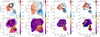 |
Fig. B.10. Same as Fig. 11 (Top-panels), but for an interacting system acting as a host galaxy (i.e. NGC 7119A). Colour bars are in the [-350,350] km s−1 and [20,350] km s−1 ranges for velocities and velocity dispersions, respectively. |
All Tables
Summary of the input parameters to simulate HARMONI observations of AGNs and their host.
Estimated effective radius at different redshifts of the galaxies acting as AGN hosts in the mock HARMONI simulations.
Stellar velocity dispersion measured from the mock HARMONI observations of representative host galaxies of AGNs at three redshifts around cosmic noon.
Number of Voronoi bins with S/N ≥ 8 in the 5100−5230 Å rest-wavelength resulting from mock HARMONI observations of the redshifted lenticular host (i.e. NGC 809) using 6, 9, 12, or 15 h (as indicated) on-source exposure times.
Basic parameters of the three nearby objects selected as models for the host galaxies of AGN at redshifts around the cosmic noon (see Sect. 3.1).
All Figures
|
Fig. 1. Key spectral features to measure MBH and σ⋆ observable at each HARMONI band as a function of the redshift. Black solid and dashed lines correspond to emission (i.e. CIV, MgII, Hβ, and Hα) and absorption (i.e. CaIIH+K, MgI, and CaII) features, respectively. The low-resolution bands correspond to the wavelength range between blue (V + R), green (I + z + J), and red (H + K) rectangles. Purple (I + z), blue (J), green (H), and red (K) filled rectangles mark the wavelength range of medium-resolution gratings. Hatch patterns mark the high-resolution bands: purple, striped, inclined: Zhigh; orange striped: Hhigh; red, striped; inclined: Kshort; and red, dashed, striped: Klong. |
| In the text | |
|
Fig. 2. Location in SFR stellar-mass diagram of the three galaxies selected as AGN hosts scaled to 1012 Lv, ⊙ (log(M⋆/M⊙)∼11.8), 1011 Lv, ⊙ (log(M⋆/M⊙)∼10.8), and 1010 Lv, ⊙ (log(M⋆/M⊙)∼9.8) luminosities. Symbols indicate the distinct hosts: circles → NGC 809, triangles → PGC 055442, and squares → NGC 7119A. The filled symbols correspond to the actual location of the three nearby galaxies (see Table A.1). At each redshift (top left labels), the solid line traces the main sequence (SFRMS) fitted by Pearson et al. (2018) (see also Table 2). Objects in the grey region correspond to quenched host galaxies. |
| In the text | |
|
Fig. 3. Theoretical QSO spectrum scaled to L[OIII] = 1043 erg s−1 in the wavelength range of interest. Emission features in the range are labelled. For reference, we also marked the location of the MgI features indicative of the host’s stellar component. |
| In the text | |
|
Fig. 4. Flux-density-to-counts ratio for the gratings (IzJ-blue and H + K-dashed red lines) used for the mock HARMONI observations of AGNs+hosts. We note that the derived functions only cover the Hβ+MgI spectral range (4770−5400 Å rest-frame wavelengths) at redshifts 0.76 (1), 1.50 (2), and 2.30 (3) due to the design of our simulations. |
| In the text | |
|
Fig. 5. PSF for HARMONI in the instrument configuration summaries in Table 3 at three wavelengths ranges. Upper panels: filter-band images (0.89−0.92 μm (left), 1.26−1.31 μm (centre), and 1.67−1.73 μm (right)). The 20 × 20 mas2 scale of our mock HARMONI observations undersamples the potential FWHM of the PSF, which varies from ∼6 mas at the bluest filter to ∼11 mas at the reddest one. Intensities are in logarithmic scale and normalised to the peak in each case. Lower panels: radial profiles along the right ascension axis and through the centre obtained from the filter-band image of the lenticular host galaxy scaled to 1011 Lv, ⊙ without QSO (black profile), the QSO of L[OIII] = 1042 (red dashed-profile), and the QSO of L[OIII] = 1043 (blue dotted-line). Intensities are normalised to the peak of the host in each case. |
| In the text | |
|
Fig. 6. Filter-band images obtained by integrating the signal of the HSIM output cubes in the spectral bands (Hβ+MgI region) of the IzJ-grating (0.82−0.93 μm (left) and 1.17−1.33 μm (centre)) and the H + K-grating (1.55−1.75 μm (right)) when considering a QSO of L[OIII] ∼ 1042 erg s−1 at the nucleus of the lenticular host (i.e. NGC 809) at redshifts 0.76 (left), 1.50 (middle), and 2.30 (right). Host luminosities are scaled to 1012 Lv, ⊙ (top), 1011 Lv, ⊙ (middle) and 1010 Lv, ⊙ (bottom). Intensity is in logarithmic scale and normalised to the peak of the brightest case (top left panel). Contours correspond to the average S/N in the rest-frame 5050−5250 Å corresponding to a stellar continuum region including the MgI features (brown contours are S/Ns of 0.06, 0.1, 0.3, and 0.6; S/Ns values of 2, 5, 9, 14, and 20 are drawn as blue contours; the purple contour indicates an S/Ns of 1). |
| In the text | |
|
Fig. 7. Same as Fig. 6, but considering a QSO of L[OIII] ∼ 1043 erg s−1 at the nucleus of the lenticular host (i.e. NGC 809). |
| In the text | |
|
Fig. 8. Full-band images obtained by integrating the signal of the HSIM output cubes in the spectral band of the IzJ (left and central; 0.81−1.34 μm) and the H + K (right; 1.45−2.40 μm) gratings when considering the lenticular host (i.e. NGC 809) as a galaxy at redshifts 0.76 (left), 1.50 (middle), and 2.30 (right) scaled to 1012 Lv, ⊙ (top), 1011 Lv, ⊙ (middle), and 1010 Lv, ⊙ (bottom) as also labelled in each panel. Intensity is in logarithmic scale and normalised to the peak of the brightest case (top left panel). As in Figs. 6 and 7, contours correspond to the average S/N in the rest-frame 5050−5250 Å (black contours are S/Ns of 0.06, 0.1, 0.3, and 0.6; S/N values of 2, 5, 9, 14, and 20 are drawn as blue contours; the purple contour indicates an S/N of 1). |
| In the text | |
|
Fig. 9. Representative spectra of lenticular host (i.e. NGC 809) at redshifts 0.76 (left), 1.50 (centre), and 2.30 (right) obtained by adding the signal from the spaxels within the effective radius (see Table 4). Top panels: spectra extracted from the HSIMInputs, only for the host galaxy scaled to 1011 Lv, ⊙. Bottom panels: spectra from the mock HARMONI observation, after reduction and flux calibration, for the three host luminosities. The blue dotted lines correspond to the PPXF best-fit model for each spectrum. |
| In the text | |
|
Fig. 10. Stellar velocity dispersion of aperture spectra obtained from the mock HARMONI observations relative to the stellar velocity dispersion of the HSIMInputs. Different symbols indicate the distinct hosts: circles → NGC 809, triangles → PGC 055442, and squares → NGC 7119A. Colours correspond to redshift and grating: blue filled symbols → z = 0.76, and IzJ grating; blue open symbols → z = 1.50, and IzJ grating; red filled symbols → z = 2.30, and HK grating. Grey dashed line marks the 20% level of uncertainty. Black dotted line indicates the typical uncertainty of σ⋆ for the HSIMInputs. Black solid line indicates σOUTPUT = σINPUT. |
| In the text | |
|
Fig. 11. Stellar kinematics of galaxies at redshifts around cosmic noon. Top panels: stellar velocity field (V⋆) and velocity dispersion distribution (σ⋆) obtained from mock HARMONI observations of three hours of on-source exposure time of lenticular (i.e. NGC 809) host galaxies scaled to the V-band luminosities indicated in each panel at redshifts 0.76 (a and b), 1.50 (c), and 2.30 (d), as also indicated. Bottom panels: same 2D-distributions but from mock HARMONI observations of six (e), nine (f and h), and 12 (g) hours of total exposure time of a lenticular hosts of the luminosities in the V band, which is labelled (i.e. 1011 L⊙ (e–g)) and 1010 L⊙ (h). Contours (in black) from the stellar continuum are overlaid in steps of 0.25 mag. For all panels, the colour bars are in the [−150,150] km s−1 and [20,200] km s−1 ranges for velocities and velocity dispersions, respectively. |
| In the text | |
|
Fig. 12. Integrated spectra for the AGN+host (lenticular galaxy) at redshifts 0.76 (left), 1.50 (centre), and 2.30 (right) obtained by adding the signal from the spaxels within the host’s effective radius (see Sect. 4.2). The labels in the top right corner indicate the host and AGN (AGN42 → 1042 and AGN43 → 1043 erg s−1) luminosities. The numbers in the top left corners indicate the S/N in the rest-frame 5050−5250 Å obtained using the der_snr algorithm. The blue-dotted lines correspond to the QSFIT model to each spectrum. Red lines draw the Gaussian profiles fitting the broad (dotted line) and narrow (dashed line) components of the emission lines in the AGN spectra. |
| In the text | |
|
Fig. 13. Full width at half maximum of the broad Hβ (left panels) and narrow [OIII]λ5007 (central panels) components of the Gaussian profiles modelling the emission lines in the AGN+hosts’ integrated-spectra at the different redshifts (see text). Right panel: equivalent-width ratio of the broad and narrow components. Different symbols indicate the distinct hosts (circles → NGC 809, triangles → PGC 055442, and squares → NGC 7119A), and their colours indicate the [OIII] luminosities of the AGN (black filled symbols → 1042, and blue open symbols → 1043 erg s−1). Error bars correspond to the uncertainties provided by the QSFIT13 package if larger than the symbol size. Dashed lines are the adopted values to simulate the emission of the central AGN (see Sect. 3.2). Grey bands indicate the parameters obtained when fitting the integrated spectra obtained from the mock HARMONI data for the pure AGN, enclosing the values and uncertainties for the two AGN luminosities. |
| In the text | |
|
Fig. A.1. Total spectra of the three nearby galaxies picked as host for our simulations of AGN+host observations with HARMONI. Spectra were normalised to the average intensity in the plotted wavelength range. The horizontal axis corresponds to rest-frame wavelengths. The spectra are shown in logarithmic scale and arbitrarily shifted on the vertical axis. Dashed-vertical lines indicate the spectral range included in the HARMONI simulations. Labels mark the position of several emission (i.e. Hβ, [O III]λ5007, HeIλ5876, [NII]λ6543, Hα, and [NII]λ6584) and absorption lines (i.e. MgIλ5163, 5172, 5183, FeIλ5269, and NaIλ5889, 5895). Dotted rectangle indicates the zoomed-in image of a region in Fig. A.5 for the NGC 7119A spectrum. |
| In the text | |
|
Fig. A.2. (a) Filter-band image of NGC 809 obtained by collapsing the MUSE data cube over the rest-frame spectral range 5100-5230 Å. (b) NGC 809 line-of-sight stellar velocity field. (c) Stellar velocity dispersion map of NGC 809. We plot all the MUSE spaxels with S/N> 1 in the 5100-5230 Å rest-frame. Limits of the colour bar are [-150,150] km s−1 and [20,200] km s−1 for velocity (panel (b)) and velocity dispersion (panel (c)), respectively. These are the same limits as those selected for the AGN hosts in Fig. 11. Contours (in black) correspond to the stellar continuum in steps of 0.25 mag. |
| In the text | |
|
Fig. A.3. Same as Fig. A.2, but for PGC 055442. Limits of the colour bar are [-180,180] km s−1 and [20,200] km s−1 for velocity (panel (b)) and velocity dispersion (panel (c)), respectively. These are the same limits as those selected for the AGN hosts in Fig. B.5. |
| In the text | |
|
Fig. A.4. Same as Fig. A.2, but for NGC 7119A. Limits of the colour bar are [-350,350] km s−1 and [20,350] km s−1 for velocity (panel (b)) and velocity dispersion (panel (c)), respectively. These are the same limits as those selected for the AGN hosts in Fig. B.10. |
| In the text | |
|
Fig. A.5. Hα+[NII]λλ6548, 6584 emission line profiles observed in the integrated spectrum of NGC 7119A. Double-peak profiles are the result of the contribution from its close companion, NGC 7119B. |
| In the text | |
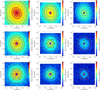 |
Fig. B.1. Same as Fig. 6, but when considering spiral morphology (i.e. PGC 055442) as a host. |
| In the text | |
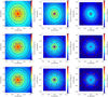 |
Fig. B.2. Same as Fig. 7, but when considering spiral morphology (i.e. PGC 055442) as a host. |
| In the text | |
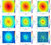 |
Fig. B.3. Same as Fig. 8, but when considering spiral morphology (i.e. PGC 055442) as a host. |
| In the text | |
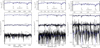 |
Fig. B.4. Same as Fig. 9, but for the considered spiral morphology (i.e. PGC 055442). |
| In the text | |
|
Fig. B.5. Same as Fig. 11 (top-panels), but for a spiral host galaxy (i.e. PGC 0055442). Colour bars are in the [-180,180] km s−1 and [20,200] km s−1 ranges for velocities and velocity dispersions, respectively. |
| In the text | |
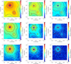 |
Fig. B.6. Same as Fig. 6, but when considering an interacting morphology (i.e. NGC 7119A) as a host. |
| In the text | |
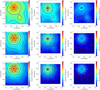 |
Fig. B.7. Same as Fig. 7, but when considering an interacting morphology (i.e. NGC 7119A) as a host. |
| In the text | |
|
Fig. B.8. Same as Fig. 8, but when considering the interacting morphology (i.e. NGC 7119A) as a host. |
| In the text | |
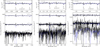 |
Fig. B.9. Same as Fig. 9, but for the considered interacting morphology (i.e. NGC 7119A). |
| In the text | |
|
Fig. B.10. Same as Fig. 11 (Top-panels), but for an interacting system acting as a host galaxy (i.e. NGC 7119A). Colour bars are in the [-350,350] km s−1 and [20,350] km s−1 ranges for velocities and velocity dispersions, respectively. |
| In the text | |
Current usage metrics show cumulative count of Article Views (full-text article views including HTML views, PDF and ePub downloads, according to the available data) and Abstracts Views on Vision4Press platform.
Data correspond to usage on the plateform after 2015. The current usage metrics is available 48-96 hours after online publication and is updated daily on week days.
Initial download of the metrics may take a while.