| Issue |
A&A
Volume 658, February 2022
|
|
|---|---|---|
| Article Number | A143 | |
| Number of page(s) | 21 | |
| Section | Astrophysical processes | |
| DOI | https://doi.org/10.1051/0004-6361/202142242 | |
| Published online | 11 February 2022 | |
Dual-frequency single-pulse study of PSR B0950+08
1
ASTRON, the Netherlands Institute for Radio Astronomy, Postbus 2, 7990 AA Dwingeloo, The Netherlands
e-mail: This email address is being protected from spambots. You need JavaScript enabled to view it.
2
LPC2E – Université d’Orléans/CNRS, 45071 Orléans Cedex 2, France
3
Station de Radioastronomie de Nançay, Observatoire de Paris, PSL Research University, CNRS, Univ. Orléans, OSUC, 18330 Nançay, France
4
National Radio Astronomy Observatory, 520 Edgemont Road, Charlottesville, VA 22903, USA
5
Institute of Physics, Eötvös Loránd University, Pázmány P. s. 1/A, 1117 Budapest, Hungary
6
Fakultät für Physik, Universität Bielefeld, Postfach 100131, 33501 Bielefeld, Germany
7
LESIA and USN, Observatoire de Paris, CNRS, PSL, SU/UP/UO, 92195 Meudon, France
8
Astro Space Center of Lebedev Physical Institute, Profsoyuznaya Str. 84/32, 117997 Moscow, Russia
9
Anton Pannekoek Institute, University of Amsterdam, Postbus 94249, 1090 GE Amsterdam, The Netherlands
10
National Centre for Radio Astrophysics, Tata Institute of Fundamental Research, Pune, 411007 Maharashtra, India
11
Cahill Center for Astronomy, California Institute of Technology, Pasadena, CA, USA
12
Netherlands eScience Center, Science Park 140, 1098 XG Amsterdam, The Netherlands
13
Department of Physics, McGill University, 3600 rue University, Montréal, QC H3A 2T8, Canada
14
McGill Space Institute, McGill University, 3550 rue University, Montréal, QC H3A 2A7, Canada
15
Max-Planck-Institut für Radioastronomie, Auf dem Hügel 69, 53121 Bonn, Germany
16
Canadian Institute for Theoretical Astrophysics, University of Toronto, 60 Saint George Street, Toronto, ON M5S 3H8, Canada
17
Dipartimento di Fisica “G. Occhialini”, Universitá degli Studi di Milano-Bicocca, Piazza della Scienza 3, 20126 Milano, Italy
18
Laboratoire Univers et Théories, Observatoire de Paris, Université PSL, CNRS, Université de Paris, 92190 Meudon, France
19
Institute of Radio Astronomy of the National Academy of Sciences of Ukraine, 4, Mystetstv St., Kharkiv 61002, Ukraine
20
AIM, CEA, CNRS, Université de Paris, Université Paris-Saclay, 91191 Gif-sur-Yvette, France
21
Dept. of Electrical Engineering, Chalmers University of Technology, Gothenburg, Sweden
22
University of Oslo Center for Information Technology, PO Box 1059 0316 Oslo, Norway
Received:
17
September
2021
Accepted:
4
November
2021
Abstract
PSR B0950+08 is a bright nonrecycled pulsar whose single-pulse fluence variability is reportedly large. Based on observations at two widely separated frequencies, 55 MHz (NenuFAR) and 1.4 GHz (Westerbork Synthesis Radio Telescope), we review the properties of these single pulses. We conclude that they are more similar to ordinary pulses of radio emission than to a special kind of short and bright giant pulses, observed from only a handful of pulsars. We argue that a temporal variation of the properties of the interstellar medium along the line of sight to this nearby pulsar, namely the fluctuating size of the decorrelation bandwidth of diffractive scintillation makes an important contribution to the observed single-pulse fluence variability. We further present interesting structures in the low-frequency single-pulse spectra that resemble the “sad trombones” seen in fast radio bursts (FRBs); although for PSR B0950+08 the upward frequency drift is also routinely present. We explain these spectral features with radius-to-frequency mapping, similar to the model developed by Wang et al. (2019, ApJ, 876, L15) for FRBs. Finally, we speculate that μs-scale fluence variability of the general pulsar population remains poorly known, and that its further study may bring important clues about the nature of FRBs.
Key words: stars: neutron
Veni Fellow.
© ESO 2022
1. Introduction
PSR B0950+08 (CP 0950, Pilkington et al. 1968) is one of the three pulsars detected in the follow-up survey of compact radio sources that was conducted after the first pulsar, CP 1919, was serendipitously discovered. The relatively large flux density and close proximity to Earth made PSR B0950+08 a subject of numerous studies, resulting in a wealth of observational facts, which were accumulated over decades. However, as is common in pulsar radio astronomy, the interpretation of this information is still subject to debate, as there is no consensus on the magnetospheric geometry, the location of radio emission, or the emission mechanism of PSR B0950+08 (e.g., Hankins & Cordes 1981).
The fluences (the spectral flux densities integrated over time) of its single pulses were quickly found to exhibit a great deal of variability (Smith 1973). Recently, a series of studies (e.g., Cairns et al. 2004; Singal & Vats 2012; Smirnova & Shishov 2008; Tsai et al. 2016; Kuiack et al. 2020) have claimed that at least some of these pulses are in fact giant pulses (GPs), a special and rare kind of pulses recorded only from a handful of pulsars. GPs are narrow (ns-μs), very bright, have a power-law fluence distribution, occur in restricted phase windows, and generally coincide with high-energy emission components (Knight 2006; Bilous et al. 2015).
In this work, we analyze single-pulse data from nonsimultaneous radio observations at two widely separated frequency ranges. We review the pulse properties and compare them both to “classical” GPs, and to the single pulses of the general pulsar population. Knowing the fluence distribution and frequency structure of single pulses of pulsar radio emission is important not only for constraining the elusive emission mechanism, but also for future pulsars searches, and for studies of fast radio bursts (FRBs).
2. Observations and data processing
This work utilizes observations recorded with Apertif on the Westerbork telescope (Adams & van Leeuwen 2019), as well as a number of dedicated low-frequency observations conducted with the NenuFAR telescope1 (Bondonneau et al. 2021; Zarka et al. 2020). Hereafter, we refer to the datasets by the Institute of Electrical and Electronics Engineers (IEEE) names of the corresponding frequency bands2, VHF for the NenuFAR 20–83 MHz band (although frequencies below 30 MHz belong to the HF IEEE band), and L-band for the 1250–1550 MHz of Apertif.
The L-band observations are comprised of seven 5-min sessions from November 2019–August 2020. These were primarily intended as short test observations that verified the Apertif system performance and real-time single-pulse detection pipeline (Sclocco et al. 2016; Connor & van Leeuwen 2018) of the ALERT FRB survey (Maan & van Leeuwen 2017). The Apertif data acquisition followed the same setup as outlined in, for example, Oostrum et al. (2020). Filterbank files were recorded with a time resolution of 81.92 μs and channels 195 kHz wide. From these, single-pulse archives were prepared with dspsr3 (van Straten & Bailes 2011) using ephemerides from the ATNF pulsar catalogue4 (Manchester et al. 2005). The number of phase bins (3080) was chosen to roughly match the filterbank time resolution. Radio frequency interference (RFI) was manually excised with the PSRCHIVE tool psrzap (Hotan et al. 2004), which resulted in zero-weighting of some of the subbands and single-pulse subintegrations. Archives were subsequently downsampled in frequency to ten subbands. In total, 18177 pulses were collected.
In the VHF band, four observations (each lasting for one hour) were carried out in January and April 2020. Coherent compensation of dispersion and Faraday rotation was applied in real time to the signal within the 8–83 MHz frequency range, using the single-pulse mode of LUPPI (the Low frequency Ultimate Pulsar Processing Instrumentation) (Bondonneau et al. 2021). The dispersion measure (DM) used for the compensation was obtained during previous observations and was subsequently refined for the correct dispersion removal in the whole band extent. In this work, we focus on the uncalibrated total intensity, as we currently lack a well-tested calibration scheme for NenuFAR data. In VHF band the time resolution was more coarse than in L-band, resulting in only 386 phase bins. In total, 53 518 pulses were examined.
All single-pulse data were next corrected for the dispersive delay due to propagation through the ionized interstellar medium (ISM). Determining the dispersion measure (DM) is not straightforward, since the L-band observations are not sensitive to small DM variations, and prominent profile evolution in the VHF band confounds the measurement of the absolute DM (Hassall et al. 2012). We used a hybrid method to make a model for profile evolution, which was then used to measure the DM for each VHF observation. The earliest VHF observation was aligned against a four-component Gaussian model in which the amplitudes and widths were all allowed to vary as a function of a frequency, but their positions were fixed (Pennucci 2015); this alignment permits a frequency-dependent separation between the two observed profile components while maintaining the usual assumption of a fixed-in-frequency fiducial point, such as the mid-point between the observed components. We then model the profile evolution in this aligned VHF observation following Pennucci (2019), in which a principal component analysis is used to reproduce the frequency dependent shape, resulting in a higher fidelity, noise-free template than when using a Gaussian component decomposition. The DM from each VHF observation was then determined by effectively measuring the ν−2 dependence of the delays of the profiles relative to this template (Pennucci et al. 2014). The DMs from the April VHF observations are ∼1σ consistent, and they are different from the January VHF DM by δDM = 5 × 10⁻⁴ pc cm−3, which amounts to a linear trend in DM of −1.8 × 10⁻³ pc cm−3 yr−1. A trend of such magnitude for a pulsar with DM ≈ 3 pc cm−3 is not uncommon (Hobbs et al. 2004; Bilous et al. 2016).
All L-band data were dedispersed using the April 2020 VHF DM value of 2.97052 pc cm−3. Assuming that the DM follows the linear trend calculated above throughout all eight months of L-band observations, the maximum pulse delay across the L-band would be ∼2 μs, much smaller than our time resolution. To each L-band observation a phase offset was applied that placed the peak of the average profile at phase 0.5. In VHF, the 0.5 phase was assigned to the dip between the two strongest components of the main profile.
3. Average profile
The average radio profile of PSR B0950+08 consists of two components, a main pulse (MP) and an interpulse (IP), separated by roughly 0.4 in spin phase (Fig. 1). In the VHF band, the MP is composed of two separate components which move further apart toward lower frequencies. The leading edge of the MP exhibits a flat shoulder (hereafter the “precursor”). The pulses originating in this precursor are known to have larger fluence variability (with respect to the average fluence in the same phase region) than the pulses from the MP (Cairns et al. 2004; Smirnova 2012).
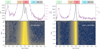 |
Fig. 1. Average profiles (upper row) and spectra (lower row) of PSR B0950+08 in VHF band (left) and L-band (right). Here, the average profiles are normalized by the mean and standard deviation of the signal in specifically selected “off-pulse-norm” window of the frequency-integrated data. The spectra are normalized by the profile maximum in each frequency subband and the logarithm of the absolute value of the signal is plotted in order to highlight faint spectral features. For the average profiles, the light purple curves show the zoom-in to the low signal-to-noise (S/N). The colored boxes at the top mark the borders of selected phase windows. These cover the interpulse (IP), precursor, main pulse (MP), off-pulse (“offp”) for the noise-induced fluence variability calculations, and another off-pulse window for baseline subtraction (“off-pulse-norm”). |
Faint emission is, notably, also present in the bridge between IP and MP, similar to the previous reports (e.g., Hankins & Cordes 1981, at 430 MHz). The bridge emission becomes relatively stronger at lower frequencies.
For the subsequent analysis we have selected five phase windows of equal width (0.15 in spin phase), which roughly cover the IP component (starting at phase 0.0), precursor (starting at 0.3), MP (0.45), and two noise windows, off-pulse (“offp”, 0.65) and off-pulse normalization (“offp-norm”, starting at 0.8). For each pulsar rotation we subtracted the mean value calculated in the off-pulse normalization window. We note that in the VHF band faint emission is present throughout virtually the full pulsar period: single-pulse fluences may thus be underestimated, and the noise contribution overestimated.
The choice of window locations was affected by our wish to have windows of the same size, to ensure the noise contribution had the same magnitude for fluences calculated in all windows. In the VHF band, the precursor window contains some emission from the MP component.
We have used uncalibrated data for this study, so we normalize the single-pulse data by the period-integrated fluence FAP of the average profile (AP), in each observing session separately. Because of the small session duration, the source elevation did not change over the observation; and the fluences averaged in 2-min rolling windows do not exhibit variation on the scales larger than ∼10 min for the longer VHF sessions (Fig. 2). Shorter-term variations in both bands can be attributed to scintillation (see Sect. 4.1).
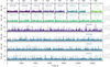 |
Fig. 2. Single-pulse fluences integrated within MP, precursor, and IP regions combined. The top two rows show L-band observations; the others correspond to the VHF sessions. Color encodes the epoch of observation, varying smoothly between darker blue (first session, November 2019) to lighter green (last session, August 2020). Grey lines mark the rolling 500-pulse average, with corresponding fluence scale displayed on the right. The observing date is noted for each session, in yymmdd format. |
4. Single-pulse properties
4.1. Long-term single-pulse fluence variability and scintillation
4.1.1. Previous studies
Numerous observing campaigns conducted at frequencies below 200 MHz have reported high variability of the flux density exhibited by PSR B0950+08 (Gupta et al. 1993; Singal & Vats 2012; Smirnova 2012; Bell et al. 2016), with occasional peaks several times higher than the average flux density. At least partly, this variation is caused by scintillation in the ISM, which thus must be taken into account when analysing single-pulse fluence distributions.
For the observations below 200 MHz, the existing measurements of the decorrelation bandwidth of the diffractive scintillation (Fig. 3) indicate that scintillation is in its strong regime (Rickett 1990). In this regime, the magnitude of the observed scintillation-induced variation of the signal depends on the number of scintles averaged within the observing bandwidth (BW) and integration time (Tintg). Such variation is commonly characterized by the modulation index, defined as the ratio of the standard deviation of the signal to its mean:
 (1)
(1)
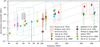 |
Fig. 3. Measurements of the decorrelation bandwidth of diffractive scintillation versus observing frequency for PSR B0950+08. For Wu et al. (in prep.), the markers at 145 MHz indicate the median as well as 2.5 and 97.5 percentiles of a series of δνDISS measurements. The width and height of the same-color rectangle around each marker shows observing bandwidth as well as minimum and maximum spectral resolution (corresponding to channel and band widths, respectively), respectively. Dashed rectangles show, in the same manner, the observing setup for three observing campaigns which did not make direct measurements of δνDISS, but reported abrupt increases in PSR B0950+08’s intensity. Dotted diagonal lines illustrate ν4 dependence. |
Following Cordes & Lazio (1991), the modulation index for diffractive scintillation can be expressed as follows:
![Mathematical equation: $$ \begin{aligned} m^{\mathrm{obs} }_{\mathrm{DISS} } \approx \left[\left(1+\kappa N_t \right)\left(1+\kappa N_\nu \right)\right]^{-1/2}, \end{aligned} $$](/articles/aa/full_html/2022/02/aa42242-21/aa42242-21-eq2.gif) (2)
(2)
where κ is an empirical factor on the order of 0.1–0.2, while Nν and Nt are the number of averaged scintles with characteristic dimensions δνDISS in frequency and δtDISS in time:
 (3)
(3)
If NνNt ≫ 1, the signal strength is distributed according to a Gaussian law with the following survival function (SF, probability of measuring a value larger than a threshold a):
 (4)
(4)
where erf is the Gauss error function. If the number of scintles averaged is small (NνNt ∼ 1), then the signal strength follows an exponential distribution with the following SF (Cordes & Lazio 1991):
 (5)
(5)
Although outliers are present, the bulk of the δνDISS measurements included in Fig. 3 suggest that between 45 and 200 MHz, δνDISS is described by the following relation:
 (6)
(6)
The measured δνDISS is smaller than predicted by Eq. (6) at 40 MHz and around 400 MHz. At the higher frequencies the values obtained in different works disagree by an order of magnitude (Cordes et al. 1985; Johnston et al. 1998; Huguenin et al. 1969). Some of this disparity may be caused by differences in observing setup, such as the session duration (maximum integration time), observing bandwidth, and frequency resolution: δνDISS is much less likely to be measured properly in cases where it is close to the band- or channel width. Similar reasoning applies to the scintillation timescale. At the same time, Kuzmin et al. (2003) reported on two δνDISS scales simultaneously present in their data at the frequencies close 100 MHz. The smaller scale is roughly in agreement with Cordes et al. (1985) and Johnston et al. (1998), adjusted for frequency evolution.
There is also an evidence of occasionally large decorrelation bandwidth. Recent wideband low-frequency observing campaigns showed that δνDISS at 145 MHz sometimes becomes as large as a few MHz, several times larger than the median value. Bell et al. (2016) reported δνDISS of 4 MHz in one of their eight observing sessions with the Murchison Widefield Array. Wu et al. (in prep.) analyzed a series of 303 observations at 145 MHz, spread over six years, using six German LOFAR stations, and found that in 2.5% of cases the δνDISS of PSR B0950+08 was larger than 3.1 MHz, with two observations yielding 5.5 ± 1 MHz. It is worth noting that a large, five-fold variation in δνDISS has been detected from another nearby pulsar, PSR J0030+0451. This variation was attributed to anisotropies in the density or the magnetic field structure of the local ISM (Nicastro et al. 2001).
Direct measurements of the scintillation timescale δtDISS at 145 MHz yield values of 15–40 min, with a larger δtDISS being generally accompanied by a larger δνDISS (Wu et al., in prep.). Bell et al. (2016) measured δtDISS = 28.8 min during their event of increased source brightness. These measurements correspond to 10–25 min at 100 MHz using the ν1.2 scaling from Lorimer & Kramer (2005), and agree well with measured δtDISS = 400 ± 100 s at 60 MHz from Smirnova & Shishov (2008).
To our knowledge, the work of Bell et al. (2016) contains the only published simultaneous measurements of flux density variations together with scintillation parameters. The latter were measured during an increased brightness event when the flux integrated for 112 s within 30-MHz bandwidth increased by a factor of 6 with respect to the flux measured during other sessions. Visually, the dynamic spectrum on their Fig. 4 contained three scintles. Using Eq. (5), for this low-scintle regime, the probability of a flux increase larger than six is e−6 ≈ 0.0025. Considering that the large δνDISS event is also quite rare, this level of variability would be quite hard to detect with only a few observing sessions.
The same holds true for Smirnova (2012) and Singal & Vats (2012). Extrapolating the possible range of scintillation parameters at 150 MHz to their frequencies of 103 MHz, we see that for the former work, Nν ∼ 1−20, Nt < 1 while for the latter, Nν ∼ 1−20, Nt ∼ 1−3. For the lowest possible number of scintles, the reported flux density variations of 6 and 8 are too strong to be described by Eq. (5) based on the number of observing sessions. On the other hand, the shape of the flux density curve versus time is similar to the low-scintle regime, with strong peaks and long troughs (Fig. 4 in Cordes & Lazio 1991). Perhaps refractive interstellar scintillation is providing extra variability. Accounting for that is difficult, since for PSR B0950+08 the long-term flux modulation indices and refractive scintillation timescales are known to deviate from the textbook predictions (Gupta et al. 1993), requiring more complex models of ISM inhomogeneties (Goldman 2021).
Diffractive scintillation may be the source of the bright 195.3-kHz spectral features of one-second snapshots during the periods of high single-pulse activity in Kuiack et al. (2020): δνDISS(60 MHz) ≈ 0.2 MHz corresponds to δνDISS(145 MHz) ≈ 6.8 MHz. This value is higher, but close to the largest δνDISS values that have been directly measured at these frequencies. We note that the exact frequency extent of the correlation in Kuiack et al. (2020) is not known very well because of the coarse resolution. A dedicated long-term study of the dynamic spectra of PSR B0950+08 below 100 MHz is needed to test the scintillation hypothesis; it is, however, indirectly corroborated by the temporal correlation of the bright features on the timescales of few minutes, similar to the measured δtDISS = 400 ± 100 s at 60 MHz (Smirnova & Shishov 2008).
4.1.2. This work
The VHF observations were carried out with a moderate frequency resolution, of 195 kHz. Although scintillation was visible in the dynamic spectrum at the top of the band, the frequency resolution was too coarse to measure the width of individual scintles with the standard autocorrelation function analysis.
In this work we investigate the fluences integrated over the 20–83 MHz frequency range. Even in the case of unusually large δνDISS of ≈0.2 MHz at 60 MHz, our band would contain dozens of scintles. Very roughly – neglecting the frequency dependence of the scintle size within the band – the modulation index for session-averaged fluence is < 0.15 and for single-pulse fluence < 0.18.
In L-band, δνDISS is much larger than our observing bandwidth and the scintillation is in its weak regime (Rickett 1990; Lorimer & Kramer 2005). The expected modulation index is 0.1–0.3 for single-pulse and session-integrated fluences.
4.2. Phase of occurrence
Figure 4 shows the distribution of the single-pulse fluences integrated over 2.6 × 10⁻³ of spin phase (equivalent to the time resolution of the VHF data), and normalized by the period-integrated mean fluence FAP of each respective session. This method of plotting highlights potential candidates for GPs: narrow pulses with fluences comparable to or exceeding FAP which come from specific phase regions, such as the leading or trailing edges of the profile components.
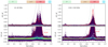 |
Fig. 4. Longitude-resolved fluence distributions per ≈650 μs, normalized by the average period-integrated fluence for each observing session. On 2D histogram, lighter colors correspond to larger number of counts in the given (phase × fluence) bin, with the darkest color corresponding to one count. The average phase-resolved fluence and its 20× and 100× multiplicatives are shown by white, red and gray lines, respectively. Spin phases beyond 0.7 are not shown. |
The brightest single pulses in our observations occur at the peak phases of the respective average profile components. The pulse-to-pulse fluence variability increases at lower frequencies in the precursor and MP regions and tentatively decreases in the IP region. In L-band, the phase-resolved fluence distribution is somewhat skewed toward the leading edge of IP and the trailing edge of MP. Such behavior is not observed in the VHF band.
We have visually inspected all periods with signal exceeding some set threshold outside on-pulse windows (0.045FAP for the VHF and 0.035FAP for L-band). In this manner, two distinct single pulses were found in the bridge region of two VHF observations. Both pulses came from the spin phase of ≈0.15, well outside the phase region for a discernible IP profile. The stronger pulse had a peak fluence of 0.064FAP, the other was 30% fainter. In both cases these are over a hundred times larger than the local average emission fluence. Both pulses had a width of about 7 ms, comparable to IP pulses and similar several-component broadband spectra (Fig. 5).
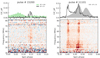 |
Fig. 5. Strongest pulse from the bridge phase region (left) and an example of a strong pulse with components in both the precursor and MP phase regions (right). Upper plot: band-integrated signal, with shaded regions marking 10× and (left only) 100× the average pulse strength. Lower plot: pulse spectrum with each frequency subband normalized by the period-integrated fluence of the average pulse in the same subband. The colorbar span is set by the maximum value on the spectrum of this particular pulse. Here and for the other VHF pulses the maximum value is calculated for frequencies above 30 MHz. |
The bridge pulses found in the VHF band bear a curious resemblance to the unusually strong pulses found by Cairns et al. (2004) at the leading edge of precursor and the trailing edge of MP component, at 430 MHz. Within 7072 pulsar rotations, the authors detected a few such pulses, one of which (corresponding to our spin phase 0.35) was more than 100 times brighter than the average profile at that phase. The pulses had width of a few ms, similar to our bridge pulses.
So far, little can be inferred about the origin of bridge pulses and whether they represent a different pulse population. Cairns et al. (2004) speculate they may be related to the micro GPs seen in the Vela pulsar (Kramer et al. 2002). Although the bridge pulses easily outshine the average emission in their respective phases, they are much dimmer than regular MP or IP single pulses. They are, furthermore, prone to being overlooked by the standard practice of only investigating single pulses in the on-pulse windows. We urge more sensitive, dedicated studies be carried out, to explore these bridge pulses further.
Our VHF observations did not confirm a few single-pulse properties that were reported previously from observations with BSA telescope in Pushchino Observatory. Smirnova (2012) noted that at 112 MHz, strong pulses in the precursor region were accompanied by an absence of emission during main pulse, and vice versa. This was interpreted as evidence supporting models in which precursor pulses are due to induced scattering of the MP emission by relativistic particles of strongly magnetized plasma in the pulsar magnetosphere (Petrova 2008). While our frequency span does not cover that of Smirnova (2012), we note that our strong precursor pulses occasionally have emission in the MP region as well (Fig. 5). Meanwhile, Kazantsev & Basalaeva (2020) reported on occurrence of strong pulses at frequencies close to 100 MHz, which come predominantly from the leading part of the two-peaked MP component. This is not supported by our observations (Fig. 4). Shabanova & Shitov (2004) observed the variations in the detected shape of the average profile with the same instrument, resulting in variable relative subcomponent height in MP, which the authors concluded to be due to Faraday rotation.
4.3. Single-pulse fluence distribution
We measured the fluences of pulses originating from the phase regions of interest, by integrating the signal within MP, precursor and IP phase regions. It is customary to normalize the fluences by the “mean pulse” fluence, although it remains a matter of choice whether to normalize by the mean fluence in the respective phase windows or by the mean fluence integrated over the whole spin period. In this work, we used period-integrated fluences calculated in each session separately, which provided uniform normalization for all three main phase regions. Individual pulse fluences can be renormalized to the average fluences of their respective phase regions by using Table 1.
Average and maximum fluences integrated within selected phase windows normalized by the average fluence integrated over the whole spin period (FAP).
The resulting band-integrated fluence histograms are shown on Fig. 6. The distribution in the off-pulse window (we note that the baseline was subtracted in a different window labeled “off-pulse-norm”) resembles a Gaussian and occupies fluences between ±0.5FAP. In both bands there is a small level of pulsar signal in the off-pulse window, so the mean fluence is somewhat larger than 0 (Table 1). The distribution of fluences from the IP window is dominated by noise and the maximum fluences are not larger than 0.8FAP. However, they are about 50 times larger than the average fluence in the IP window, indicating the largest degree of variability among three emission windows. This degree must be taken with caution, since at this low level of average fluence its exact value is affected by details of baseline subtraction. Unlike MP, IP emission shows more variability at higher frequencies.
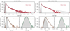 |
Fig. 6. Fluence histograms for three selected phase windows (color lines). Fluences are normalized by the average profile fluence integrated over whole period during the respective observing session. The distribution of fluences in the off-pulse window is shown with gray shade. For off-pulse window, gray dashed line indicates normal distribution based on mean and standard deviation of fluences integrated over this window. For main pulse and precursor window, the best-fit convolution of lognormal and Gaussian noise distributions is shown with black line (see text for details). |
Although some VHF pulses in the precursor window have flux density values larger than 100× the average flux density in the exact same phase window, their integrated fluences are only up to 20 times larger. The L-band data shows less fluence variability. For the MP phase region, the distribution in L-band appear to steepen at F ≳ 5FAP, however relatively strong pulses with F ≳ 8FAP are also present. Interestingly enough, the fluence distribution at 430 MHz from Hankins & Cordes (1981) also shows steepening at similar fluences, and the shape of the distributions are qualitatively similar.
Following a procedure similar to Burke-Spolaor et al. (2012), we fit the observed MP and precursor fluence distributions with lognormal distributions (Pintrinsic) convolved with a Gaussian model for the off-pulse region:
 (7)
(7)
Poffp was approximated with the probability density function of the normal distribution, with μN and σN measured directly from the data:
![Mathematical equation: $$ \begin{aligned} \mathrm{N} (\mu _\mathrm{N} , \sigma _\mathrm{N} ) \sim \frac{1}{\sigma _\mathrm{N} }\exp \left[-\frac{(F/F_\mathrm{AP} -\mu _\mathrm{N} )^2}{2\sigma _\mathrm{N} ^2}\right]. \end{aligned} $$](/articles/aa/full_html/2022/02/aa42242-21/aa42242-21-eq14.gif) (8)
(8)
The off-pulse flux density distribution appeared reasonably well described by the normal distribution, with some excess of pulses on both tails of the Gaussian curve, which we attribute to residual RFI. Because of this excess the formal reduced χ2, defined as sum of squared difference between model and data in the fluence bins with at least one pulse:
 (9)
(9)
was rather high (> 4); we chose to proceed with a Gaussian model because of its simplicity.
The intrinsic flux density distribution was modeled with log-normal (LN) distribution, with the same parametrization as in Burke-Spolaor et al. (2012):
![Mathematical equation: $$ \begin{aligned}&P_\mathrm{intrinsic} \equiv \mathrm{LN} (\mu _\mathrm{LN} , \sigma _\mathrm{LN} )\nonumber \\&\qquad \quad \sim \frac{F_\mathrm{AP} }{F\sigma _\mathrm{LN} } \exp \left[ -\frac{[\log _{10}(F/F_\mathrm{AP} )-\mu _\mathrm{LN} ]^2}{2\sigma _\mathrm{LN} ^2} \right]. \end{aligned} $$](/articles/aa/full_html/2022/02/aa42242-21/aa42242-21-eq16.gif) (10)
(10)
The convolution of Pintrinsic and best-fit Poffp (Eq. (7)) was fit to the observed histogram Pobserved by minimizing the χ2 statistics from Eq. (9).
The fit results are given in Table 2. The minimum reduced χ2 value was sensitive to the number of bins in the fluence histogram and was generally higher for the smaller number of bins. The much larger reduced χ2 value for the precursor window in L-band is mostly caused by the small number of bins per extent of the distribution. Increasing bin number results in similar best-fit parameter values, but a reduced χ2 comparable to the distributions from the other windows. For the MP window in L-band, χ2 indicates only a marginally good lognormal fit if we follow the χ2 = 2.8 threshold accepted by Burke-Spolaor et al. (2012). However, our best-fit values of μLN and σLN are outliers in the distribution of corresponding quantities from Burke-Spolaor et al. (2012). None of their lognormal fluence distributions have μLN < 0. This could, in particular, stem from the different fluence normalizations we adopted: we normalize MP fluences by total mean FAP, including signal from IP and precursor. Re-fitting the distribution of MP fluences normalized by the average in MP phase window increases μLN, but it still remains negative. On the other hand, σLN is larger than almost all of corresponding values on Burke-Spolaor et al. (2012) sample, indicating an unusually large variability of the single-pulse fluences of PSR B0950+08.
From the visual estimation in VHF, the fit underestimates the number of high-fluence pulses (we note that bins with one pulse were not used in χ2 minimization). In L-band there is a shortage of pulses with moderate fluences (6–12FAP, same as in Hankins & Cordes 1981), but the lognormal distribution still predicts the highest observed fluence correctly. It must be kept in mind that many factors may distort the true shape of single-pulse fluence distribution: non-Gaussian noise, contamination of MP fluences by precursor pulses, broadband intensity variations of the dispersed signal in VHF, scintillation, etc. The influence of these factors is generally hard to quantify, since it depends on the observing setup, preprocessing, and exact ways of calculating fluences. Nevertheless, some rough estimates may be derived from comparing fluence distributions obtained in different works at similar radio frequencies. Detailed discussion is given in Sect. 5.1, however we may state that unless for some reasons the fluence distributions are considerably offset from each other, at the same level of incidence probabilities the single-pulse fluences from different works may differ by up to ∼25%.
4.4. Pulse spectra
A number of examples of individual pulse spectra from the strongest pulses in MP, precursor and IP regions are shown in Fig. 7. In L-band the spectra do not exhibit any noticeable frequency dependence over the 300 MHz bandwidth. The spectrum of the strongest, 12-FAP pulse (#3232) does not have any special features, compared to other MP pulses. The strongest pulses from precursor and IP region are much weaker than the MP pulses, but their spectra do not seem to be qualitatively different.
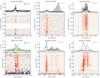 |
Fig. 7. Pulses with largest fluence in IP (left), precursor (middle) and MP (right column). Top row: L-band, bottom row: VHF. For the plotting conventions, see the caption to Fig. 5. |
In the VHF band, the moderate time resolution did not allow us to explore the fine features of individual pulses on the same timescale as in L-band. Also, spectra of individual pulses below roughly 40 MHz are affected by approximately minute-long broadband fluctuations of the pulsar signal, possibly due to refraction or scintillation in the Earth ionosphere, or telescope issues (Song et al. 2018; Fallows et al. 2016). After compensating for dispersive delay, these intensity fluctuations manifest themselves as narrowband, bright patches that move upward in frequency, across several pulsar periods (Fig. 8). Thus, any low-frequency bright spots on individual spectra must be interpreted with caution.
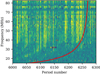 |
Fig. 8. Dynamic spectra for 300 pulse periods, averaged in MP+precursor phase region. Color is saturated. Red line shows dedispersed track for DM = 0. |
Below 100 MHz, many pulses appeared to consist of subpulses of limited bandwidth, which drifted upward on the leading edge of MP and downward on its trailing edge (Fig. 9). Sometimes a downward (but no upward) drift was observed in the precursor region. This frequency drift is different from the artifacts caused by broadband variation of dispersed signal, as it happens on much smaller timescale and can go both ways in frequency. The strongest pulses from the IP and bridge phase regions (Figs. 5 and 7) consist of broadband components with no sign of frequency drift. The small number of strong pulses does not, however, allow us to draw any definitive conclusions on the prevalence of the drift.
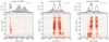 |
Fig. 9. Examples of subpulses drifting in frequency in precursor and MP. For the plotting conventions, see the caption to Fig. 5. |
The positions of low-frequency subpulses do not seem to shift away from each other at low frequencies in a manner similar to components of the average profile (Fig. 1). Interestingly, this same behavior was previously noticed during narrowband simultaneous low-frequency observations: Rickett et al. (1975) and Rickett & Cordes (1981) reported that micropulse positions are highly correlated between 111 and 318 MHz and that the distance between them remains frequency-independent.
In our observations, the spectra of individual pulse components had widths of ≳30 MHz. We can conjecture that the spectral width is frequency-dependent and gradually increases with frequency. According to Rickett et al. (1975), individual micropulses have wideband spectra spanning at least from 111 to 318 MHz and in L-band they are larger than our band width of 300 MHz.
5. Discussion
5.1. Comparison of fluence distribution to the literature
In the literature, precursor single pulses were rarely explored separately. Also, at the lowest frequencies, these precursor single pulses may extend into the MP phase region (Fig. 5). Therefore, in order to compare the single-pulse fluence distributions from our observations to previous work, we integrated fluences within the combined MP and precursor windows, and normalized these by the total AP fluence (we note that the average fluence in MP+precursor is 95% and 98% of the FAP in VHF and L-band, respectively: normalizations by FAP and the average flux in MP+precursor are almost identical). The survival functions for individual sessions did not differ significantly from each other (Fig. 10). On a log-log scale, the SFs exhibited a smooth, curved shape, affected by thermal noise below F0 ≈ 2FAP.
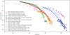 |
Fig. 10. Survival function of the PSR B0950+08 single-pulse fluence distribution in the MP+precursor phase regions, from our observations and literature. For our observations, dark and light green circles mark the combined distribution in L-band and individual sessions, respectively. Similarly, light and dark red circles show the distributions for the VHF fluences. One-second continuum integrations from Kuiack et al. (2020), equivalent to 4-pulse fluence sums, are shown with blue circles and squares. Orange triangles mark single-pulse fluences from Tsai et al. (2016). Purple circles and squares mark the measurements of Singal & Vats (2012), with lighter shade showing values renormalized to their local average profile fluences. Observations from Smirnova (2012) are shown as unfilled magenta circles. Power-law indices from the literature or this work are given next to the corresponding distributions in matching color. |
We did not attempt to identify an exact functional form of the distribution, since for L-band the limited total observing duration resulted in only a moderate range of recorded fluences; while in VHF the broadband intensity fluctuations may obscure the true SF shape. For the sake of comparison with the literature, we fit a collection of broken power laws (PLs) to our distributions. We fit α(Fmin, Fmax) such that the survival function of the fluence distribution in the fluence range Fmin/FAP < F ≤ Fmax/FAP was described by
 (11)
(11)
The results of the fit are given in Table 3. The literature single-pulse fluence SFs are collected in Fig. 10. All were constructed from pulses at 100 MHz or below and should thus be compared to our VHF observations. Some authors (e.g., Tsai et al. 2016) normalized single-pulse fluences by FAP measured in the same session. Others such as Singal & Vats (2012) used FAP averaged over many sessions. Finally, Smirnova & Shishov (2008) provided calibrated fluences. Further details on these literature distributions are found in Appendix A.1. Interestingly, the distributions at similar radio frequencies tend to agree with each other, if the fluences are normalized by the local average fluence of the session for the work of Smirnova & Shishov (2008) and one session in Singal & Vats (2012). For another session in Singal & Vats (2012), the reported average flux is too low and normalized fluence distribution is offset from the bulk of other measurements, albeit having roughly the same slope.
Comparing SFs with Kuiack et al. (2020) requires special care because their result is an SF of continuum fluences integrated within one second (≈4P). These SF are constructed by counting the number of events above a set threshold and dividing it by the number of pulsar periods in all sessions combined, not the number of one-second integrations. While Kuiack et al. (2020) remark that their SFs are dominated by single pulses, we find this not to be valid for the range of probabilities explored in their work. We simulated a distribution with the power-law probability density function equivalent to the SF of the observed pulses (with index −5, see Fig. 10), and find that the probability that SF constructed from four-element sums matches the individual-element SF is smaller than 10−8. Given the number of pulses included in Kuiack et al. (2020), their smallest possible probability is 10−6. The effect is further illustrated by distribution of fluences from consecutively summed 4 pulses in our VHF band (Fig. 11), normalized by total number of pulses to match Kuiack et al. (2020). For all probabilities smaller than ≈0.2 the distribution for fluences integrated within one second is shifted to the right with respect to single-pulse distribution. Thus, we have to compare the distributions from Kuiack et al. (2020) to our four-pulse distributions.
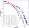 |
Fig. 11. Single-pulse MP+precursor fluence survival functions from all sessions of VHF observations combined (red circles) together with 4-P sums of fluences normalized by total number of periods (triangles). The latter SF emulates observing setup of Kuiack et al. (2020) who integrated continuum fluence in one-second (4P) intervals, but constructed SF by normalizing by total number of periods in their session. The distributions of fluences from Kuiack et al. (2020) are shown as the shades of blue for the normalization provided by the authors and as shades of gray with normalization of 2.5 larger FAP (see text for details). |
The SFs from Kuiack et al. (2020) have similar shape to ours, but their single-pulse fluences are approximately 2.5 larger. Their work measures continuum flux, which includes an unpulsed component that is entirely missed by the traditional pulsar observing setup that we use. Ruan et al. (2020) reported on unpulsed flux of PSR B0950+08 to be 0.59 ± 0.16 Jy at 74 MHz, with, so far, a poorly constrained spectral index. While the corresponding fluence should be subtracted from the measured by Kuiack et al. (2020), it is likely to only be a minor correction.
Kuiack et al. (2020) do not themselves measure the average fluence, extrapolating it from the flux density measurements of Tsai et al. (2016). For PSR B0950+08, the flux density measurements in the 20–170 MHz frequency range exhibit a considerable amount of variation (Fig. 12). For frequencies below 100 MHz the measurements were made over the course of one or few hours, or over some number of sessions. It is possible that the scatter of the reported flux density values is partly influenced by scintillation, and partly by systematic flux calibration errors. Individual observations at frequencies above 100 MHz exhibit a great deal of variation, with flux increases by a factor of a few, and in this variation scintillation is likely to play a considerable role (see Sect. 4.1).
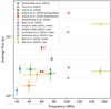 |
Fig. 12. Average flux density spectrum for PSR B0950+08 constructed from the literature with uncertainties given by the authors (Zakharenko et al. 2013; Tsai et al. 2015, 2016; Bondonneau et al. 2020; Ruan et al. 2020; Singal & Vats 2012; Smirnova & Shishov 2008; Bell et al. 2016). The horizontal errorbars indicate bandwidth. For observations at frequencies higher than 100 MHz both mean and maximum fluxes per observing campaign are shown. Kuiack et al. (2020) did not measure the average flux density values directly, but extrapolated from Tsai et al. (2016). The question mark points to the conjectured flux density value that would align the single-pulse fluence distribution of Kuiack et al. (2020) with other work (Figs. 10 and 11). |
The distributions from Kuiack et al. (2020) can be made to match our 4-P sums if we assume the average flux during their observing epoch was actually about 2.5× higher than the normalization value that was used (based on Tsai et al. 2016). Considering the overall uncertainty on the average flux density, possible intrinsic flux variability, and the influence of scintillation for a given observing setup, it is difficult to assess whether the true average flux during this observation could have been 6.2 Jy, rather than the 2.6 Jy that was assumed. The scintillation timescale at their frequencies should be ∼5–14 min, compatible with the flux density variation scale from their Fig. 5 (i.e., the figure does not provide clear evidence of the contrary). A potential, unusually large δνDISS would make the instantaneous modulation index to be close to 0.6–0.7, making the observed fluence distribution more shallow. However, over the four-hour observations the average flux density would have a modulation index of 0.2–0.5, meaning it is not likely the average flux over the session as whole would be increased. Clearly, more observations are needed to investigate this matter. These should include simultaneous measurements of single-pulse fluence distributions, calibrated average fluence and, preferably, direct scintillation measurements.
5.2. On the possibility of PSR B0950+08 emitting GPs
The single-pulse variability of the first few dozens of pulsars, studied in 1970s at frequencies above 100 MHz, lacked single pulses brighter than ten times the average intensity (see references in Cognard et al. 1996). The subsequently discovered strong pulses from PSR B1937+21 and the Crab pulsar painted a sharp contrast. Thsese high-intensity pulses seemingly followed a separate distribution, suggesting a distinct pulse population. Such pulses were named “giant pulses” and, for the time being, the “ten times the average” criterion discriminated between the two populations5. Several other pulsars joined the GP-emitting set, their GPs roughly sharing the following properties: ns-μs width, high brightness temperature, restricted window of occurrence coinciding with high-energy emission, strong magnetic field at the light cylinder. This led to the speculation of GPs being associated with caustic radio emission produced close to the light cylinder (see review in Bilous et al. 2015). In this paper, we call such GPs “classical GPs”.
While there has been some progress in constraining single-pulse fluence distributions on a population level (Burke-Spolaor et al. 2012; Mickaliger et al. 2018) since the 1970s, much of the field is still there to explore. At the same time a plethora of peculiar single-pulse variability patterns has been discovered, including, but not limited to giant micropulses (μs-wide, F > 10FAP for longitude-resolved fluence only, PL energy distribution with indices similar to those of GPs, see Johnston & Romani 2002; Cairns et al. 2004; Raithel et al. 2015); individual pulses from sparsely radio-emitting neutron stars (“rotating radio transients”, RRATs McLaughlin et al. 2006), which are wider than GPs and have a lognormal fluence distribution (Keane et al. 2010; Mickaliger et al. 2018); RRAT-like pulses from normal pulsars (e.g., Esamdin et al. 2012), “bursting modes” characterized by abrupt onset, changes in the shape of the single-pulse fluence distribution and the shape of the average profile (e.g., Seymour et al. 2014; Wang et al. 2020); prolonged periods of absence of any emission (nulling, resulting in very low values of average flux, see, for example, Gajjar et al. 2014). At low radio frequencies of ≲100 MHz single-pulse fluences seem to be more variable, resulting in regular detection of ms-wide pulses above the 10FAP GP threshold (Kuzmin 2007; Ulyanov et al. 2006).
In this section we try to compare some properties of single pulses from PSR B0950+08 to GPs and to “normal” pulses. The task is somewhat complicated by the absence of clear definition of a “giant” or a “not a giant” pulse and the dearth of sufficient observational knowledge to distinguish between the two classes. It is also possible that these two classes are mere extremes and in fact pulsars’ single-pulse properties form a continuum.
5.2.1. Fluence distribution
In our L-band observations of PSR B0950+08, only one pulse in the MP+precursor region exceeds the historical 10FAP threshold. This pulse occurred in the middle of the MP window. Its shape and spectrum resembled the other, less energetic single pulses we observe. If we compare to the average fluence only in the occurrence phase window, all three phase regions exhibited single pulses above this factor-10 threshold. None of those bright pulses in the MP or precursor region, however, appeared to have properties (such as widths, pulse shapes and spectra) distinctly different from the fainter pulses. For the IP, the generally low signal-to-noise ratio (S/N) of individual pulses precludes drawing any similar conclusions, although individual IP pulses definitely show the most variability with respect to their average. At the same time, peak flux densities occasionally exceed 20× absolute or local peak flux density of the average pulse, especially for the IP region. In the VHF data, single-pulse fluences exhibit a greater degree of variability in MP and precursor, but smaller in the IP, but the trend described above remains the same: pulses above 10FAP threshold do not have properties visibly distinct from fainter pulses.
Let us discuss how does the single-pulse fluence variability of PSR B0950+08 compare to the rest of the pulsar population. As discussed in Sect. 4.3, a lognormal distribution provides a marginally good fit to the single-pulse fluences from the MP and precursor regions. The best-fit coefficients indicate an unusually large degree of variability (more shallow SF), when compared to other pulsars with lognormal single-pulse fluence distributions from the 315-pulsar L-band study by Burke-Spolaor et al. (2012). It is worth noting that among 225 non-nulling pulsars, only 33% had a log-normal single-pulse fluence distribution, while 48% were classified as “other”, that is neither Gaussian, lognormal nor bimodal. Burke-Spolaor et al. (2012) also revealed that for their brightest sources (approximately 20% of the total sample, regardless of distribution shape) the fluence distribution integrated within the on-pulse window did not exceed 6.4FAP. Taking into account the distribution of single-pulse counts collected in their sample, our L-band observations suggest a larger degree of fluence variability.
Mickaliger et al. (2018) explored observations in the frequency range similar to the one of Burke-Spolaor et al. (2012) and analyzed a partly overlapping source sample of a similar size, albeit with roughly an order of magnitude more observing time. Interestingly, 58% of sources showed single pulses with fluences F > 10FAP, with a probability of getting by chance such a large fluence values ranging from 10−4.5 to 10−1.5. About 16% of the sources exceeded 20FAP, with approximately the same probability range. The L-band single-pulse fluence distribution for PSR B0950+08 that we report here falls well within the sample SFs from Mickaliger et al. (2018), not showing any signs of unusual single-pulse fluence variability.
The tentative inconsistency between Mickaliger et al. (2018) and Burke-Spolaor et al. (2012) is puzzling and might be at least partially explained with different source samples and observing time. Ultimately, a larger study of single-pulse fluences is needed both in L-band and at low frequencies. For the low frequencies, there has been no population study of single-pulse fluence distributions yet, so we do not really know the typical degree of single-pulse fluence variability. We hypothesize that single-pulse fluences become increasingly more variable at lower frequencies, however for PSR B0950+08 the SF still lies within the Mickaliger et al. (2018) sample.
Let us discuss how do the single-pulse fluences for PSR B0950+08 compare to “classical” GPs. Figure 13 shows GP fluence distributions from studies that measured both the average flux and the GP flux (see details in Appendix A.3). Three things can immediately be gleaned from Fig. 13. First of all, the SFs of GPs are more shallow than those of normal pulses and they seem to follow PL distributions for a larger fractional range of fluences (many show flattening at lower fluences, due to intrinsic properties, or to observing artifacts such as incomplete sampling near the selection threshold, or noise influence). Secondly, the fluence distribution for the “classical” GPs is on average much better studied due to dedicated long-term observations. However, one must keep in mind that most of these observations were performed after bright pulses caught attention, so there is a strong selection bias present. In this regard, it would be very interesting to explore the high-fluence tails of the distributions from Mickaliger et al. (2018). Finally, it is interesting to note that, when normalized by their respective FAP, most of the GP distributions continue below 10FAP and that for the same SF probabilities the relative fluences from different pulsars span two orders of magnitude. Obviously, if GPs were a separate pulse population and do not contribute much to FAP, normalizing them by FAP is to some extent arbitrary.
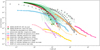 |
Fig. 13. Comparison of PSR B0950+08’s MP+precursor fluence distribution to the sample of normal pulsars from Mickaliger et al. (2018, light green lines) and the collection of “classical” GPs normalized to FAP (colored lines). Other measurements of the PSR B0950+08 single-pulse fluence distributions from Fig. 10 are given in gray (using the same markers as in that Figure). |
On the log-log scale the distribution of single-pulse fluences from PSR B0950+08 is steeper than that of GPs and generally can be fit with a single PL over a smaller range of fluences. However, neglecting the fluence offset between our distribution and the one of Kuiack et al. (2020) and combining two distributions together produces a seemingly-PL distribution spanning an order of magnitude in pulse fluence and four orders of magnitude in probability, which is similar to known GP distributions, albeit with the steeper slope. Interestingly, PSR B1957+21 exhibits a similar PL slope over a similar span in magnitude in its low mode, and has a clear flattening of at the large-fluence end, in the high mode. It is yet unclear whether these low-mode single pulses are GPs in the classical sense.
It is currently unknown which form of distribution, lognormal or PL, better describes the high-fluence tail of the fluence distribution (or the full distribution) for single pulses from PSR B0950+08, other “normal” pulsars and GPs. Careful studies of such kind are required.
Finally, we note that a fluence offset between distributions from different authors, as observed for PSR B0950+08 (Fig. 10), is also present for the GP fluence distributions of the two most studied GP emitters, the Crab pulsar and PSR B1937+21. Most of the works on GPs from these pulsars provide only fluences of individual GPs, not the average profile. While the slope of the PL fit is similar at similar observing frequencies (e.g., references in Mickaliger et al. 2012; Knight et al. 2006), the fluences of GPs at similar probabilities are different by a factor of few or even a few orders of magnitude (Fig. 14). These discrepancies may be only partly explained by scintillation, and we believe they may stem from unaccounted systematic errors in flux density calibration or from intrinsic variability. In any case such a large uncertainty in the rate of occurrence of a GP of specific fluence has considerable influence on the estimates of prospects of detecting GPs from pulsars beyond our Galaxy.
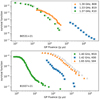 |
Fig. 14. Survival function of the fluence distributions for two most studied GP pulsars, the Crab pulsar PSR B0531+21 and PSR B1937+21 from the works of Bhat et al. (2008, B08), Bera & Chengalur (2019, B19), Karuppusamy et al. (2010, K10), McKee et al. (2019, M19), Kinkhabwala & Thorsett (2000, K00), and Soglasnov et al. (2004, S04). The gray unfilled markers show fluences rescaled to a common frequency (1.3 GHz for the Crab and 1.4 GHz for PSR B1937+21) using broadband spectral fits from Bilous et al. (2016) and Kondratiev et al. (2018). |
5.2.2. Pulse duration and brightness temperature
Because of their high peak-flux density and narrow widths, GPs sometimes have the largest implied brightness temperatures among all known astrophysical sources: Tb > 5 × 1039 K for PSR B1937+21 (Soglasnov et al. 2004), 1037 K or even 1041 K for the Crab pulsar (Hankins et al. 2003; Hankins & Eilek 2007). However, such measurements are anecdotal since they require a special observing setup and can be performed only on strong pulses at the frequencies where pulses are unaffected by scattering. For the same Crab pulsar, Tb is several orders of magnitude lower when time resolution is larger than the duration of pulse or its subcomponents (1032 K, Cordes et al. 2004).
Individual pulses of PSR B0950+08 are much wider than “classical” GPs, and typically even have widths comparable to that of the average profile components. At the same time, observing with sufficient time resolution reveals that individual pulses are often composed of a collection of separate μs-wide subpulses (micropulses, also dubbed “microstructure”, e.g., Hankins 1971). Micropulses have been recorded from a substantial fraction of strong nearby pulsars and are speculated to be a common trait of pulsar radio emission (Lange et al. 1998; Popov et al. 2002; Kuzmin et al. 2003; De et al. 2016). Their origin is still as unknown as the GP formation mechanism; although some studies link these phenomena (Petrova 2004a,b). Most existing studies of the microstructure focus on the quasi-periodicity of micropulses (e.g., Cordes et al. 1990), and, as of now, the other properties of micropulses (e.g., fluence distribution, polarization) are not known well enough to compare them thoroughly to “classical” GPs.
In our study pulsar emission was recorded with rather coarse time resolution, which precluded studying PSR B0950+08’s microstructure, especially in the VHF band. We still observe sharp single-pulse components both in VHF and L-band (Figs. 7 and 9). The brightest such component in L-band peaked at 0.3FAP. Assuming average flux in L-band to be 100 mJy (Jankowski et al. 2018), this indicates the peak flux density of 91 Jy and Tb ∼ 1027 K for the effective width equal to 81.92 μs time resolution. This is much smaller than the typical Tb of GPs, however it is currently unclear what the smallest timescale present in the PSR B0950+08’s microstructure is, and how bright individual subpulses can be. Hankins & Boriakoff (1978) reported a strong (1 kJy) sub-μs unresolved subpulse at 430 MHz, with implied Tb > 3 × 1031 K. At the same time Popov et al. (2002), observing for an hour at 1.6 GHz with time resolution of only 62.5 ns did not find any subpulses shorter than few μs.
5.2.3. Constraints on the place of origin
Observed single pulses from PSR B0950+08 contribute directly to its average emission. Thus, one can use the average profile to constrain the emission altitudes with the help of radius-to-frequency mapping and the rotating vector model (Radhakrishnan & Cooke 1969; Kijak & Gil 2003). An apparent average-profile bifurcation below 400 MHz is a common feature, interpreted as emission coming from the diverging magnetic field lines. Within the core/cone emission region model (Rankin 1990, 1993), the presence of interpulse emission means that we observe either two poles of an orthogonal rotator or a very wide cone of an almost aligned one. Both models appear to have difficulties explaining the observed data (Hankins & Cordes 1981). Fitting a rotating vector model to polarization data, and modeling magnetospheric X-ray emission, preferred an orthogonal rotator (Everett & Weisberg 2001; Becker et al. 2004), but a series of works employing more sophisticated beam shapes spoke in favor of an aligned one (e.g., Narayan & Vivekanand 1983; Gil 1983). Thus, standard techniques do not provide an unambiguous picture of the magnetic field configuration and the emission heights in PSR B0950+08, since no model explains all observed characteristics.
While the region of the GP origin is still unknown, GP phase windows are hinted to be associated with average-profile components thought to be made of caustic radio waves emitted close to the light cylinder (LC). The high magnetic field strengths on the LC for the “classical” GP pulsars may be important for their emission mechanism (e.g., Lyubarsky 2019). Caustic radio components coincide with X-ray and gamma-ray emission. For PSR B0950+08, nonthermal magnetospheric X-rays are indeed observed, however the peaks of X-ray profile are substantially offset from the radio peaks, speaking against caustic origin of the radio components (Becker et al. 2004). In γ-rays PSR B0950+08 has not been detected yet – it is absent from the most recent Fermi Large Area Telescope Fourth Source Catalog (Abdollahi et al. 2020), although no targeted search has been published either. Finally, its magnetic field on the light cylinder, calculated using the standard dipole magnetic field model, is several orders of magnitude smaller than those of classical GP pulsars.
The frequency evolution of the profile components in the VHF band can, however, be qualitatively explained by geometrical models which involve diverging magnetic field lines (see Sect. 5.3), thus speaking against an LC origin. It is interesting to note that no direct comparison can be made between VHF pulses observed in PSR B0950+08, and the classical GPs at the same frequencies. To our knowledge, only the Crab pulsar has individual GPs recorded below 200 MHz (Popov et al. 2006; Eftekhari et al. 2016; Karuppusamy et al. 2012; van Leeuwen et al. 2020), however scattering in the ISM precludes any studies of pulse structure at these frequencies. The rest of “classical” GP pulsars show similar or larger levels of scattering and are generally fainter than Crab GPs.
5.3. What can PSR B0950+08 tell us about FRBs
Fast radio bursts (FRBs) are sub-ms radio pulses of extragalactic origin (Lorimer et al. 2007; see Petroff et al. 2019, 2021 for the recent reviews). As the precise nature of FRBs is yet to be determined, dozens of theories abound to explain their properties (cf. the theory catalog from Platts et al. 2019). Magnetospheres of neutron stars are popular candidates for FRB origin. Non-cataclysmic, repeating FRBs are for example being attributed to super-GPs from young neutron stars or MSPs (Cordes & Wasserman 2016; Connor et al. 2016). Recently, an extremely bright (but still few orders of magnitude fainter than the bulk of extragalactic FRBs) radio burst was detected from a Galactic magnetar SGR J1935+2154 (Bochenek et al. 2020), accompanied by two much fainter bursts (Kirsten et al. 2020).
Repeating FRBs often show so-called “sad trombone” behavior, downward drifting time-frequency structures (examples from Apertif are found in Pastor-Marazuela et al. 2021). Quite strikingly, the spectral features of PSR B0950+08 strongly resemble these structures – although the trombones are actually quite “happy” on the leading side of the MP (Fig. 9). Wang et al. (2019) and Lyutikov (2019) proposed a geometric explanation for such sad trombones in FRBs, by examining the radiation from groups of charged particles in a neutron star magnetosphere, in the classical framework of pulsar radio-to-frequency mapping (Fig. 15). In this framework, clumps of plasma emit radio waves tangentially to the field lines they propagate along. Higher radio frequencies are generated closer to the stellar surface (which is natural if emission is due to curvature radiation). In the model of Wang et al. (2019), a sudden release of energy creates the required, separate, charged clumps, and these propagate along neighboring field lines. As the neutron star rotates, our line of sight (LOS) fortuitously first cuts through the high-frequency emission from one of these clumps, at the lower altitude; then later cuts through the lower-frequency emission from another clump at higher altitude; thus creating apparent downward frequency drift (Fig. 15A). This model would not create upward frequency drift if all clumps are created simultaneously, since clumps propagate away from the stellar surface (Fig. 15B). On the other hand, one can imagine that for pulsars, clumps are created more regularly and that our LOS, passing through the leading half of the on-pulse window, can first pick up low-frequency emission from one batch of clumps and then high-frequency emission from another, resulting in apparent upward frequency drift (Fig. 15C). Interestingly, single pulses form PSR B0950+08’s precursor show downward frequency drift, thereby complicating the interpretation of precursor emission within classical core/cone model. We note that this model is purely geometrical and does not specify the exact mechanism for charged plasma or radio emission generation – these may be different for rotation-powered pulsars and magnetars.
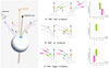 |
Fig. 15. Cartoon model of the frequency drift in subpulse components in pulsars and FRBs from the radius-to-frequency mapping of emission from separate plasma clumps propagating in neutron star magnetosphere (Wang et al. 2019). The inset on the left side shows neutron star with magnetic dipole axis (black arrow) inclined with respect to the spin axis (orange arrow). The light blue circle on the surface of the star shows the footpoints of the open field lines, with a couple of field lines drawn as an example. Purple dashed arrows indicate LOS direction. Following classical radius-to-frequency mapping, radio waves are emitted tangentially to the field line, with higher frequencies coming from smaller altitudes. The emission is postulated to come from a ring of field lines with the same magnetic collatitude. As pulsar rotates, the observer detects emission from a range altitudes at the moments of time t1−4 (black dots). In the center column the 2D projection of the same setup is shown with magnetic dipole axis lying in the picture plane and the spin axis pointing up and away from the reader. The line of sight (LOS) at t1−2 or t3−4 is indicated by the dotted line. Pulse spectra are plotted in the rightmost column. In all three rows some event generates clumps of plasma simultaneously on two separate field lines. These clumps are moving along the field lines emitting radio waves with altitude-dependent radio frequency. For the row (A) LOS fortuitously aligns with radio emission from one clump at higher radio frequency, and, shortly afterward, with another clump at lower frequency, resulting in the “sad trombone” spectrum. For (B) the same scenario is shown for the leading part of the profile. In this case the clump is not there yet when LOS passes through outer magnetic field line, resulting in single-component “no trombone” spectrum. For pulsars (C) clumps are supposed to be much more frequent (but still distinct), so LOS crosses beams of radio waves from two different batches of clumps, generating upward frequency drift, a.k.a. “happy trombone”. |
To our knowledge, “normal” emission from radio pulsars was never considered as a potential explanation for FRB emission because of the vast disparity in luminosities and brightness temperatures. Figure 16 shows that disparity on the duration versus luminosity diagram that is common to the field. However, we must note that there is much more variability to pulsar emission than is traditionally acknowledged. Single-pulse fluence distributions are not constrained well on a population level and single pulses exceeding 10× or 100× the mean fluence may not be as rare as previously thought. Also, very little is known about the fluence distribution of pulsar microstructure. Those scarce records of microstructure fluences from ordinary nearby pulsars that do exist – recorded within hours or even minutes-long sessions! – show brightness temperatures which are quite different from the averages that are generally reported.
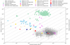 |
Fig. 16. Time-luminosity phase-space plot for radio pulses from neutron stars and repeating FRBs showing the product of observing frequency and pulse width (νW in GHz s) against equivalent isotropic spectral luminosity (4πSpeakd2, left) and the pseudoluminosity (Speakd2, right). The brightness temperature Tb = (1/2kb)×(Speakd2)/(νW)2 is indicated by gray lines. Black dots show pulsar spectral luminosity calculated from continuum flux density at 1400 MHz, with pulse duration assumed to be full width at half maximum of the average profile at the same frequency (ATNF pulsar catalog v.1.64 Manchester et al. 2005) or 0.04P if no such value was given in the catalog. Lighter dots mark common single-pulse fluence variability at 10× the average pulse luminosity. Light green diamonds show FRBs from repeating sources with known distances (FRB 20121102A, FRB 20180916B, FRB 20190711A, FRB 20200120E see Nimmo et al. (2021), and references therein). Purple pentagon mark individual bursts from magnetar SGR 1935+2154 taken from compilation by Nimmo et al. (2021), and the downward triangles indicate the average pulse luminosities from the neutron stars with surface magnetic field larger than 5 × 10¹³ G in the ATNF catalog. Stars show representative GPs or their components from the studies where both peak flux density and widths were measured, with the latter not biased by scattering (but still possibly below time resolution). Light blue color marks the Crab pulsar (Hankins et al. 2003; Hankins & Eilek 2007; Karuppusamy et al. 2010; Popov et al. 2009; Bera & Chengalur 2019; Bhat et al. 2008), beige corresponds to PSR B1937+21 (Kinkhabwala & Thorsett 2000; Soglasnov et al. 2004; McKee et al. 2019), yellow to PSR B1821-24A (Knight et al. 2006; Bilous et al. 2015), pink to PSR B0540-69 (Geyer et al. 2021), and light violet to PSR B1957+21 (Main et al. 2017). Finally, upward red triangle shows unresolved microstructure component for PSR B0950+08 from Hankins & Boriakoff (1978). Blue upward triangles mark strong microcomponents from a pulse from another ordinary nearby PSR B1133+16 (Bartel 1978; Bartel & Hankins 1982). The brightest unresolved component for our L-band observation of PSR B0950+08 is shown with the red square (see text for details). Downward triangles of corresponding colors show the average pulses from the respective pulsars. |
With the discovery of much fainter bursts from the repeating sources FRB 20180916B and FRB 20200120E, and the “FRB-emitting” galactic magnetar SGR J1935+2154 (see Nimmo et al. 2021, and references therein), the question of neutron-star radio emission variability attracts renewed attention. Perhaps the individual pulses from neutron stars occupy a large fraction of the parameter space between GPs, average pulses and FRBs, and some of the latter are caused by extreme cases of the mechanism that operates in the magnetospheres of ordinary pulsars.
Finally, we note the curious but striking similarities in individual pulse morphology when we compare PSR B0950+08 with a single burst from the repeating FRB 20180916B and with a pulse from magnetar XTE J1810−197 (Fig. 17). The peculiar shape of PSR B0950+08’s single pulses were best described by Hankins & Cordes (1981): “sometimes amorphous noisy pulses, sometimes very “spiked” micropulses interspersed with regions where the signal returns briefly to the system noise level, and occasional quasi-periodic micropulses”. The observations of PSR B0950+08 performed at 18–26 MHz by Ulyanov et al. (2016) revealed an interesting spectral behavior in one of the pulses recorded. A sequence of four ms-spaced subpulse components had visible dispersion difference between the pairs of components #1/3 and #2/4 (Fig. 18). Similar behavior was recently noticed in one of the pulses from repeating FRB 20180916B, at frequencies an order of magnitude higher (Pleunis et al. 2021). Ulyanov et al. (2016) attributed the difference in visible dispersion measure to propagation through turbulent plasma in the neutron star magnetosphere and pulsar wind. It would be interesting to test this theory on FRB data.
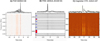 |
Fig. 17. Apparent similarities in pulse morphology between radio pulses from PSR B0950+08, a repeating FRB source and a magnetar. Left: one of single pulses from B0950+08 (this work). Middle: burst from repeating FRB 20180916B (Marcote et al. 2020). Right: somewhat scattered single pulse from magnetar XTE J1810−197 (PSR J1809−1943; Maan et al. 2019). In all three cases there is present the combination of amorphous structure and sharp peaks, with drops down to the noise level in between. |
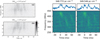 |
Fig. 18. Interesting spectral structure of an individual pulse from PSR B0950+08 observed at the very low radio frequencies by Ulyanov et al. (2016, left) and of a burst from repeating FRB 20180916B observed at higher frequencies (Pleunis et al. 2021, right). |
6. Summary
We have analyzed nonsimultaneous single-pulse observations of PSR B0950+08 in two widely separated frequency regions. Although coarse frequency resolution did not allow us to measure ISM parameters in our study, we argue that some of the high fluence variability that was previously reported is due to the changing decorrelation bandwidth on our LOS. Similarly to Cairns et al. (2004), we found a distinct pair of pulses pulse in the bridge region between MP and IP, with very low average level of emission.
Comparing the fluence distributions and other properties of the PSR B0950+08’s single pulses to those of “classical” GPs and “normal” pulses suggests that PSR B0950+08 does not emit GPs, although the exact location of emission region remains elusive. We argue that the pulse population labeled by Kuiack et al. (2020) as separate and brighter may have been mischaracterized due to normalization with a noncontemporary average flux density from the literature, and we point out common mismatches in the GP energies reported by various authors.
Finally, we present upward and downward frequency drifts in single pulses below 100 MHz, and argue that the geometrical model of “sad trombones” from FRBs may be applicable here. We conclude that little is actually known about the μs-scale fluence variability of normal pulsars, and that its further study may bring important clues about the nature of FRBs.
A threshold 2× higher is also extensively used in the literature, and flux density integration methods varies: average fluence in the whole on-pulse window, in a given component, in a phase window of GPs, peak flux density and so on.
Acknowledgments
A.B. thanks M. Mickaliger and S. Burke-Spolaor for help in retrieving the single-pulse energy distributions reported in their works, K. Nimmo for comments on the time-luminosity phase-space plot, and A. Rohatgi for creating web based tool to extract data from plots. This research was supported by the European Research Council under the European Union’s Seventh Framework Programme (FP/2007-2013)/ERC Grant Agreement No. 617199 ‘ALERT’, and by NWO, the Dutch Research Council, under Vici research programme ‘ARGO’ with project number 639.043.815 (PI:JvL). JPWV acknowledges support by the Deutsche Forschungsgemeinschaft (DFG) through the Heisenberg programme (Project No. 433075039). GS acknowledges financial support provided under the European Union H2020 ERC Consolidator Grant “Binary Massive Black Hole Astrophysics” (B Massive, Grant Agreement: 818691). DV acknowledges support from the Netherlands eScience Center (NLeSC) under grant ASDI.15.406. EP acknowledges funding from an NWO Veni Fellowship. J.W.K. is a CITA Postdoctoral Fellow: This work was supported by the Natural Sciences and Engineering Research Council of Canada (NSERC), [funding reference #CITA 490888-16]. This paper is partially based on data obtained using the NenuFAR radio-telescope. The development of NenuFAR has been supported by personnel and funding from: Station de Radioastronomie de Nançay, CNRS-INSU, Observatoire de Paris-PSL, Université d’Orléans, Observatoire des Sciences de l’Univers en Région Centre, Région Centre-Val de Loire, DIM-ACAV and DIM-ACAV+ of Région Ile-de-France, Agence Nationale de la Recherche. We acknowledge the use of the Nançay Data Center computing facility (CDN – Centre de Données de Nançay). The CDN is hosted by the Station de Radioastronomie de Nançay in partnership with Observatoire de Paris, Université d’Orléans, OSUC and the CNRS. The CDN is supported by the Région Centre-Val de Loire, département du Cher. The Nançay Radio Observatory is operated by the Paris Observatory, associated with the French Centre National de la Recherche Scientifique (CNRS). This work makes use of data from the Apertif system installed at the Westerbork Synthesis Radio Telescope owned by ASTRON. ASTRON, the Netherlands Institute for Radio Astronomy, is an institute of NWO. Apertif instrumentation development for this research was supported by NWO (grant 614.061.613 ‘ARTS’) and the Netherlands Research School for Astronomy (‘NOVA4-ARTS’, ‘NOVA-NW3’, and ‘NOVA5-NW3-10.3.5.14’). We thank Apertif Builders E. A. K. Adams, B. Adebahr, W. A. van Cappellen, W. J. G. de Blok, J. P. R. de Reijer, B. S. Frank, J. E. Hargreaves, K. M. Hess, E. Kooistra, D. M. Lucero, Á. Mika, J. Morawietz, R. Morganti, V. A. Moss, M. J. Norden, T. A. Oosterloo, E. Orrú, A. A. Ponomareva, G. W. Schoonderbeek, A. Sclocco, R. van der Brink, J. M. van der Hulst, D. van der Schuur, G. N. J. van Diepen, M. A. W. Verheijen, and S. J. Wijnholds.
References
- Abbate, F., Bailes, M., Buchner, S. J., et al. 2020, MNRAS, 498, 875 [CrossRef] [Google Scholar]
- Abdollahi, S., Acero, F., Ackermann, M., et al. 2020, ApJS, 247, 33 [Google Scholar]
- Adams, E. A. K., & van Leeuwen, J. 2019, Nat. Astron., 3, 188 [Google Scholar]
- Bartel, N. 1978, A&A, 62, 393 [NASA ADS] [Google Scholar]
- Bartel, N., & Hankins, T. H. 1982, ApJ, 254, L35 [NASA ADS] [CrossRef] [Google Scholar]
- Becker, W., Weisskopf, M. C., Tennant, A. F., et al. 2004, ApJ, 615, 908 [NASA ADS] [CrossRef] [Google Scholar]
- Bell, M. E., Murphy, T., Johnston, S., et al. 2016, MNRAS, 461, 908 [NASA ADS] [CrossRef] [Google Scholar]
- Bera, A., & Chengalur, J. N. 2019, MNRAS, 490, L12 [NASA ADS] [CrossRef] [Google Scholar]
- Bhat, N. D. R., Tingay, S. J., & Knight, H. S. 2008, ApJ, 676, 1200 [Google Scholar]
- Bilous, A. V., Pennucci, T. T., Demorest, P., & Ransom, S. M. 2015, ApJ, 803, 83 [NASA ADS] [CrossRef] [Google Scholar]
- Bilous, A. V., Kondratiev, V. I., Kramer, M., et al. 2016, A&A, 591, A134 [NASA ADS] [CrossRef] [EDP Sciences] [Google Scholar]
- Bochenek, C. D., Ravi, V., Belov, K. V., et al. 2020, Nature, 587, 59 [NASA ADS] [CrossRef] [Google Scholar]
- Bondonneau, L., Grießmeier, J. M., Theureau, G., et al. 2020, A&A, 635, A76 [NASA ADS] [CrossRef] [EDP Sciences] [Google Scholar]
- Bondonneau, L., Grießmeier, J. M., Theureau, G., et al. 2021, A&A, 652, A34 [NASA ADS] [CrossRef] [EDP Sciences] [Google Scholar]
- Burke-Spolaor, S., Johnston, S., Bailes, M., et al. 2012, MNRAS, 423, 1351 [Google Scholar]
- Cairns, I. H., Johnston, S., & Das, P. 2004, MNRAS, 353, 270 [NASA ADS] [CrossRef] [Google Scholar]
- Cognard, I., Shrauner, J. A., Taylor, J. H., & Thorsett, S. E. 1996, ApJ, 457, L81 [NASA ADS] [Google Scholar]
- Connor, L., & van Leeuwen, J. 2018, AJ, 156, 256 [NASA ADS] [CrossRef] [Google Scholar]
- Connor, L., Sievers, J., & Pen, U.-L. 2016, MNRAS, 458, L19 [Google Scholar]
- Cordes, J. M., & Lazio, T. J. 1991, ApJ, 376, 123 [NASA ADS] [CrossRef] [Google Scholar]
- Cordes, J. M., & Wasserman, I. 2016, MNRAS, 457, 232 [NASA ADS] [CrossRef] [Google Scholar]
- Cordes, J. M., Weisberg, J. M., & Boriakoff, V. 1985, ApJ, 288, 221 [NASA ADS] [CrossRef] [Google Scholar]
- Cordes, J. M., Weisberg, J. M., & Hankins, T. H. 1990, AJ, 100, 1882 [CrossRef] [Google Scholar]
- Cordes, J. M., Bhat, N. D. R., Hankins, T. H., McLaughlin, M. A., & Kern, J. 2004, ApJ, 612, 375 [NASA ADS] [CrossRef] [Google Scholar]
- De, K., Gupta, Y., & Sharma, P. 2016, ApJ, 833, L10 [NASA ADS] [CrossRef] [Google Scholar]
- Eftekhari, T., Stovall, K., Dowell, J., Schinzel, F. K., & Taylor, G. B. 2016, ApJ, 829, 62 [NASA ADS] [CrossRef] [Google Scholar]
- Esamdin, A., Abdurixit, D., Manchester, R. N., & Niu, H. B. 2012, ApJ, 759, L3 [NASA ADS] [CrossRef] [Google Scholar]
- Everett, J. E., & Weisberg, J. M. 2001, ApJ, 553, 341 [NASA ADS] [CrossRef] [Google Scholar]
- Fallows, R. A., Bisi, M. M., Forte, B., et al. 2016, ApJ, 828, L7 [NASA ADS] [CrossRef] [Google Scholar]
- Gajjar, V., Joshi, B. C., & Wright, G. 2014, MNRAS, 439, 221 [CrossRef] [Google Scholar]
- Geyer, M., Serylak, M., Abbate, F., et al. 2021, MNRAS, 505, 4468 [NASA ADS] [CrossRef] [Google Scholar]
- Gil, J. 1983, A&A, 127, 267 [NASA ADS] [Google Scholar]
- Goldman, I. 2021, MNRAS, 504, 4493 [NASA ADS] [CrossRef] [Google Scholar]
- Gupta, Y., Rickett, B. J., & Coles, W. A. 1993, ApJ, 403, 183 [NASA ADS] [CrossRef] [Google Scholar]
- Hankins, T. H. 1971, ApJ, 169, 487 [NASA ADS] [CrossRef] [Google Scholar]
- Hankins, T. H., & Boriakoff, V. 1978, Nature, 276, 45 [CrossRef] [Google Scholar]
- Hankins, T. H., & Cordes, J. M. 1981, ApJ, 249, 241 [NASA ADS] [CrossRef] [Google Scholar]
- Hankins, T. H., & Eilek, J. A. 2007, ApJ, 670, 693 [Google Scholar]
- Hankins, T. H., Kern, J. S., Weatherall, J. C., & Eilek, J. A. 2003, Nature, 422, 141 [CrossRef] [Google Scholar]
- Hassall, T. E., Stappers, B. W., Hessels, J. W. T., et al. 2012, A&A, 543, A66 [NASA ADS] [CrossRef] [EDP Sciences] [Google Scholar]
- Hobbs, G., Lyne, A. G., Kramer, M., Martin, C. E., & Jordan, C. 2004, MNRAS, 353, 1311 [NASA ADS] [CrossRef] [Google Scholar]
- Hotan, A. W., van Straten, W., & Manchester, R. N. 2004, Proc. Astron. Soc., 21, 302 [NASA ADS] [CrossRef] [Google Scholar]
- Huguenin, G. R., Taylor, J. H., & Jura, M. 1969, Astrophys. Lett., 4, 71 [NASA ADS] [Google Scholar]
- Jankowski, F., van Straten, W., Keane, E. F., et al. 2018, MNRAS, 473, 4436 [Google Scholar]
- Johnston, S., & Romani, R. W. 2002, MNRAS, 332, 109 [NASA ADS] [CrossRef] [Google Scholar]
- Johnston, S., Nicastro, L., & Koribalski, B. 1998, MNRAS, 297, 108 [NASA ADS] [CrossRef] [Google Scholar]
- Johnston, S., Romani, R. W., Marshall, F. E., & Zhang, W. 2004, MNRAS, 355, 31 [NASA ADS] [CrossRef] [Google Scholar]
- Karuppusamy, R., Stappers, B. W., & van Straten, W. 2010, A&A, 515, A36 [NASA ADS] [CrossRef] [EDP Sciences] [Google Scholar]
- Karuppusamy, R., Stappers, B. W., & Lee, K. J. 2012, A&A, 538, A7 [NASA ADS] [CrossRef] [EDP Sciences] [Google Scholar]
- Kazantsev, A. N., & Basalaeva, M. Y. 2020, ArXiv e-prints [arXiv:2005.07244] [Google Scholar]
- Keane, E. F., Ludovici, D. A., Eatough, R. P., et al. 2010, MNRAS, 401, 1057 [NASA ADS] [CrossRef] [Google Scholar]
- Kijak, J., & Gil, J. 2003, A&A, 397, 969 [NASA ADS] [CrossRef] [EDP Sciences] [Google Scholar]
- Kinkhabwala, A., & Thorsett, S. E. 2000, ApJ, 535, 365 [Google Scholar]
- Kirsten, F., Snelders, M. P., Jenkins, M., et al. 2020, Nat. Astron. [Google Scholar]
- Knight, H. S. 2006, Chin. J. Astron. Astrophys. Suppl., 6, 41 [CrossRef] [Google Scholar]
- Knight, H. S., Bailes, M., Manchester, R. N., Ord, S. M., & Jacoby, B. A. 2006, ApJ, 640, 941 [NASA ADS] [CrossRef] [Google Scholar]
- Kondratiev, V., Bilous, A.& LOFAR PWG 2018, in Pulsar Astrophysics the Next Fifty Years, eds. P. Weltevrede, B. B. P. Perera, L. L. Preston, & S. Sanidas, 337, 358 [NASA ADS] [Google Scholar]
- Kramer, M., Johnston, S., & van Straten, W. 2002, MNRAS, 334, 523 [Google Scholar]
- Kuiack, M., Wijers, R. A. M. J., Rowlinson, A., et al. 2020, MNRAS, 497, 846 [NASA ADS] [CrossRef] [Google Scholar]
- Kuzmin, A. D. 2007, in WE-Heraeus Seminar on Neutron Stars and Pulsars 40 years after the Discovery, eds. W. Becker, & H. H. Huang, 72 [Google Scholar]
- Kuzmin, A. D., Hamilton, P. A., Shitov, Y. P., et al. 2003, MNRAS, 344, 1187 [CrossRef] [Google Scholar]
- Lange, C., Kramer, M., Wielebinski, R., & Jessner, A. 1998, A&A, 332, 111 [NASA ADS] [Google Scholar]
- Lorimer, D. R., & Kramer, M. 2005, Handbook of Pulsar Astronomy (Cambridge University Press) [Google Scholar]
- Lorimer, D. R., Bailes, M., McLaughlin, M. A., Narkevic, D. J., & Crawford, F. 2007, Science, 318, 777 [Google Scholar]
- Lyubarsky, Y. 2019, MNRAS, 483, 1731 [NASA ADS] [CrossRef] [Google Scholar]
- Lyutikov, M. 2019, ArXiv e-prints [arXiv:1908.07313] [Google Scholar]
- Maan, Y., & van Leeuwen, J. 2017, in 2017 XXXIInd General Assembly and Scientific Symposium of the International Union of Radio Science (URSI GASS), 2 [Google Scholar]
- Maan, Y., Joshi, B. C., Surnis, M. P., Bagchi, M., & Manoharan, P. K. 2019, ApJ, 882, L9 [Google Scholar]
- Mahajan, N., van Kerkwijk, M. H., Main, R., & Pen, U.-L. 2018, ApJ, 867, L2 [NASA ADS] [CrossRef] [Google Scholar]
- Main, R., van Kerkwijk, M., Pen, U.-L., Mahajan, N., & Vanderlinde, K. 2017, ApJ, 840, L15 [NASA ADS] [CrossRef] [Google Scholar]
- Manchester, R. N., Lyne, A. G., Camilo, F., et al. 2001, MNRAS, 328, 17 [NASA ADS] [CrossRef] [Google Scholar]
- Manchester, R. N., Hobbs, G. B., Teoh, A., & Hobbs, M. 2005, AJ, 129, 1993 [Google Scholar]
- Marcote, B., Nimmo, K., Hessels, J. W. T., et al. 2020, Nature, 577, 190 [NASA ADS] [CrossRef] [Google Scholar]
- McKee, J. W., Stappers, B. W., Bassa, C. G., et al. 2019, MNRAS, 483, 4784 [NASA ADS] [Google Scholar]
- McLaughlin, M. A., Lyne, A. G., Lorimer, D. R., et al. 2006, Nature, 439, 817 [NASA ADS] [CrossRef] [Google Scholar]
- Mickaliger, M. B., McLaughlin, M. A., Lorimer, D. R., et al. 2012, ApJ, 760, 64 [Google Scholar]
- Mickaliger, M. B., McEwen, A. E., McLaughlin, M. A., & Lorimer, D. R. 2018, MNRAS, 479, 5413 [Google Scholar]
- Narayan, R., & Vivekanand, M. 1983, ApJ, 274, 771 [NASA ADS] [CrossRef] [Google Scholar]
- Nicastro, L., Nigro, F., D’Amico, N., Lumiella, V., & Johnston, S. 2001, A&A, 368, 1055 [NASA ADS] [CrossRef] [EDP Sciences] [Google Scholar]
- Nimmo, K., Hessels, J. W. T., Kirsten, F., et al. 2021, ArXiv e-prints [arXiv:2105.11446] [Google Scholar]
- Oostrum, L. C., Maan, Y., van Leeuwen, J., et al. 2020, A&A, 635, A61 [NASA ADS] [CrossRef] [EDP Sciences] [Google Scholar]
- Pastor-Marazuela, I., Connor, L., van Leeuwen, J., et al. 2021, Nature, 596, 505 [NASA ADS] [CrossRef] [Google Scholar]
- Pennucci, T. T. 2015, PhD Thesis, University of Virginia [Google Scholar]
- Pennucci, T. T. 2019, ApJ, 871, 34 [NASA ADS] [CrossRef] [Google Scholar]
- Pennucci, T. T., Demorest, P. B., & Ransom, S. M. 2014, ApJ, 790, 93 [NASA ADS] [CrossRef] [Google Scholar]
- Petroff, E., Hessels, J. W. T., & Lorimer, D. R. 2019, A&ARv, 27, 4 [NASA ADS] [CrossRef] [Google Scholar]
- Petroff, E., Hessels, J. W. T., & Lorimer, D. R. 2021, ArXiv e-prints [arXiv:2107.10113] [Google Scholar]
- Petrova, S. A. 2004a, A&A, 424, 227 [NASA ADS] [CrossRef] [EDP Sciences] [Google Scholar]
- Petrova, S. A. 2004b, A&A, 417, L29 [NASA ADS] [CrossRef] [EDP Sciences] [Google Scholar]
- Petrova, S. A. 2008, MNRAS, 384, L1 [Google Scholar]
- Pilkington, J. D. H., Hewish, A., Bell, S. J., & Cole, T. W. 1968, Nature, 218, 126 [NASA ADS] [CrossRef] [Google Scholar]
- Platts, E., Weltman, A., Walters, A., et al. 2019, Phys. Rep., 821, 1 [NASA ADS] [CrossRef] [Google Scholar]
- Pleunis, Z., Michilli, D., Bassa, C. G., et al. 2021, ApJ, 911, L3 [NASA ADS] [CrossRef] [Google Scholar]
- Popov, M. V., Bartel, N., Cannon, W. H., et al. 2002, A&A, 396, 171 [NASA ADS] [CrossRef] [EDP Sciences] [Google Scholar]
- Popov, M. V., Kuz’min, A. D., Ul’yanov, O. M., et al. 2006, Astron. Rep., 50, 562 [NASA ADS] [CrossRef] [Google Scholar]
- Popov, M., Soglasnov, V., Kondratiev, V., et al. 2009, PASJ, 61, 1197 [NASA ADS] [CrossRef] [Google Scholar]
- Radhakrishnan, V., & Cooke, D. J. 1969, Astrophys. Lett., 3, 225 [NASA ADS] [Google Scholar]
- Raithel, C. A., Shannon, R. M., Johnston, S., & Kerr, M. 2015, ApJ, 804, L18 [NASA ADS] [CrossRef] [Google Scholar]
- Rankin, J. M. 1990, ApJ, 352, 247 [Google Scholar]
- Rankin, J. M. 1993, ApJ, 405, 285 [Google Scholar]
- Rickett, B. J. 1990, ARA&A, 28, 561 [NASA ADS] [CrossRef] [Google Scholar]
- Rickett, B. J., & Cordes, J. M. 1981, in Pulsars: 13 Years of Research on Neutron Stars, eds. W. Sieber, & R. Wielebinski, 95, 107 [NASA ADS] [Google Scholar]
- Rickett, B. J., Hankins, T. H., & Cordes, J. M. 1975, ApJ, 201, 425 [NASA ADS] [CrossRef] [Google Scholar]
- Ruan, D., Taylor, G. B., Dowell, J., et al. 2020, MNRAS, 495, 2125 [NASA ADS] [CrossRef] [Google Scholar]
- Sclocco, A., van Leeuwen, J., Bal, H. E., & van Nieuwpoort, R. V. 2016, Astron. Comput., 14, 1 [NASA ADS] [CrossRef] [Google Scholar]
- Seymour, A. D., Lorimer, D. R., & Ridley, J. P. 2014, MNRAS, 439, 3951 [CrossRef] [Google Scholar]
- Shabanova, T. V., & Shitov, Y. P. 2004, A&A, 418, 203 [NASA ADS] [CrossRef] [EDP Sciences] [Google Scholar]
- Singal, A. K., & Vats, H. O. 2012, AJ, 144, 155 [NASA ADS] [CrossRef] [Google Scholar]
- Smirnova, T. V. 2012, Astron. Rep., 56, 430 [Google Scholar]
- Smirnova, T. V., & Shishov, V. I. 2008, Astron. Rep., 52, 736 [NASA ADS] [CrossRef] [Google Scholar]
- Smith, F. G. 1973, MNRAS, 161, 9P [NASA ADS] [CrossRef] [Google Scholar]
- Soglasnov, V. A., Popov, M. V., Bartel, N., et al. 2004, ApJ, 616, 439 [Google Scholar]
- Song, X., Kondratiev, V., & Bilous, A. 2018, in Pulsar Astrophysics the Next Fifty Years, eds. P. Weltevrede, B. B. P. Perera, L. L. Preston, & S. Sanidas, IAU Symp., 337, 412 [Google Scholar]
- Tsai, J.-W., Simonetti, J. H., Akukwe, B., et al. 2015, AJ, 149, 65 [NASA ADS] [CrossRef] [Google Scholar]
- Tsai, W. J., Simonetti, J. H., Akukwe, B., et al. 2016, AJ, 151, 28 [NASA ADS] [CrossRef] [Google Scholar]
- Ulyanov, O. M., Zakharenko, V. V., Konovalenko, O. O., et al. 2006, Russ. Radio Phys. Radio Astron., 11, 113 [NASA ADS] [Google Scholar]
- Ulyanov, O. M., Skoryk, A. O., Shevtsova, A. I., Plakhov, M. S., & Ulyanova, O. O. 2016, MNRAS, 455, 150 [NASA ADS] [CrossRef] [Google Scholar]
- van Leeuwen, J., Mikhailov, K., Keane, E., et al. 2020, A&A, 634, A3 [NASA ADS] [CrossRef] [EDP Sciences] [Google Scholar]
- van Straten, W., & Bailes, M. 2011, PASA, 28, 1 [Google Scholar]
- Wang, W., Zhang, B., Chen, X., & Xu, R. 2019, ApJ, 876, L15 [NASA ADS] [CrossRef] [Google Scholar]
- Wang, S. Q., Hobbs, G., Wang, J. B., et al. 2020, ApJ, 902, L13 [NASA ADS] [CrossRef] [Google Scholar]
- Zakharenko, V. V., Vasylieva, I. Y., Konovalenko, A. A., et al. 2013, MNRAS, 431, 3624 [NASA ADS] [CrossRef] [Google Scholar]
- Zarka, P., Denis, L., Tagger, M., et al. 2020, in URSI GASS 2020, Session J01 New Telescopes on the Frontier [Google Scholar]
Appendix A: Details on fluence distributions from the literature
A.1. PSR B0950+08
Kuiack et al. (2020) recorded bright emission from PSR B0950+08 using AARTFAAC, an imaging transient detection instrument at LOFAR. A sample of 275 one-second snapshot images with fluences ranging from 42 to 177 kJy ms were collected during 96 hours of observations in 1.5-MHz bands centered at 58.3 and 61.8 MHz. The time resolution was thus 4 times larger than the pulse period. The normalizing AP fluence is obtained from interpolation over the average flux density values at nearby frequencies obtained in earlier studies at other telescopes.
Singal & Vats (2012) carried out 141 32-min observing sessions with the Rajkot telescope. Pulsed emission from PSR B0950+08 was recorded over 1.6 MHz of bandwidth centered at 103 MHz. A single linear polarization was received and the sampling time was 48 ms (thus, covering all of MP window). Over the time of observations, the mean pulse intensity was 3 Jy, however the pulsar displayed a great deal of variability, between < 0.3 Jy and 26 Jy. The authors used a 30-Jy criterion for bright pulse selection. The authors note that there is almost one-to-one correspondence between the rate of the strong pulses and the average pulse intensity of the session. The survival functions for three sessions are shown, with intensity of the pulses normalized by mean intensity (3 Jy). We note that since the MP window is not resolved, these are essentially fluences. Two of these sessions are from 1998, for which the average intensity per session is shown on their Fig. 3. For Feb 28 (59th day of the year), the mean flux is 24 Jy, for March 17 (day 76) it is 13 Jy.
Smirnova (2012) observed PSR B0950+08 with the Large Scanning Antenna of the Pushchino Radio Astronomy Observatory at 112 MHz with 2.3-MHz bandwidth. One component of the polarized emission was received and the Faraday rotation was not removed. The fluence distribution shown was compiled for pulses from three sessions with the highest S/N of the average profile. The duration of each session was about 765 pulse periods. In their Sec. 3, the authors note that 30-Jy peak flux density corresponds to the 2 Jy average flux density. Using this relation, we can convert the average peak flux density of the three brightest sessions (130 Jy) to the average fluence of 2.2 Jy s. This fluence value was used for normalization on Fig. 10, however we note that there is a factor of two difference in peak fluxes between the most and the least bright sessions in the sample. Also, the fluence in Smirnova (2012) was calculated in windows with edges at 0.3 of the peak flux of each given pulse, which may lead to some underestimation of single-pulse fluence as compared to using fixed-phase windows.
Tsai et al. (2016) recorded three 4-hr sessions on consecutive days with the Low Wavelength Array (LWA1). Observations were performed in the beamformed mode at 42 and 74 MHz, each with a bandwidth of 16 MHz. Because of changing elevation of the source the System Equivalent Flux Density of the telescope changed by approximately 30% over the course of each session. The authors fit Gaussians to single pulses and the average profile and report the ratio of the areas under the fit curves for individual and average pulse (thus, essentially, fluences). The authors searched for pulses using different DMs and smoothing time series with boxcars of different widths. They did not record fluences in each period. All pulses with fluences larger than ten of AP are shown in their work.
A.2. Population studies
Mickaliger et al. (2018) compiled single-pulse distributions for 264 pulsars and RRATs using 35-min pointings from the Parkes Multi-Beam Pulsar Survey (Manchester et al. 2001). The survey was conducted in 288-MHz bandwidth centered at 1374 MHz. For each pointing, the authors identified an on- and off-pulse windows on the folded profile, subtracted the off-pulse mean in each spin period and integrated single-pulse fluences (FSP) within the on-pulse window. These fluences were normalized by the fluence of the average profile of the pointing (hereafter, we denote them as F ≡ FSP/FAP). The influence of thermal noise was not explored.
Unfortunately, only the plots of fluence distributions were preserved (Mickaliger, priv. comm.). As input to our study, those plots (259 pulsars, RRATs omitted) were downloaded from the referenced web page6 and manually digitized using a web-based tool7. On the figures, fluence distributions were displayed as non-normalized histograms on the log-log scale. Logarithms of normalized fluences were binned with fixed-width bins, where the bin width and fluence range varied from pointing to pointing.
Using the obtained values of N(Fi) in bins with centers at Fi and constant widths ΔF, we constructed the survival functions as:
 (A.1)
(A.1)
where Nperiods is number of spin periods per pointing.
A fraction of pulsars was observed more than once; the respective SFs were combined. As a sanity check we note that for all but one source, the SFs at the lowest fluence were smaller than one. That is expected, since the log-scale plots could not show periods where noise variations produced F < 0. The only plot with SF(F0) > 1, for PSR J1822-0848, potentially contained data from the wrong source.
The precision of this manual digitization process was assessed by comparing the retrieved values for the total numbers of pulses at the high-fluence end of the distribution, to the expected number. For 1912 counts with N < 5, the median of N/round(N) was 0.97 and 68% range was [0.90, 1.03]. This we assume to be the fractional error for both F and N(F).
A.3. Giant pulses
Abbate et al. (2020) explored the properties of GPs from PSR B1820−30A. The authors used the MeerKAT radio telescope in South Africa to record two 150-min (≈3.1 × 10⁶P total) sessions at 1284 MHz with 642-MHz bandwidth. The authors measure the peak S/N of GPs in time series with 10 μs resolution and normalize it by the total S/N of the integrated profile by the square root of the number of rotations observed. GPs come from the phase regions of components C1 and C2 (there is also much weaker C3 component). The authors note that some of their GPs had multiple one-bin peaks. On Fig. 13 we show pulses from main profile component (“C1”, 13522 GPs total). GPs from component C2 have distribution with similar slope, but are order of magnitude less frequent.
Bhat et al. (2008) recorded GPs from the Crab pulsar with the Australian Compact Telescope Array at 1300 MHz (32-MHz bandwidth) during one session. Fluences were calculated in custom windows around each GP. The distribution for MP and IP giant pulses are combined. The authors estimate that uncertainties in fluence estimates depend on the pulse strength and width, ranging from 0.5% for strong and narrow pulses, to 35% for the weak and broad pulses.
Bilous et al. (2015) studied the fluence distribution of GPs from PSR B1821−24A. The authors combined pulses from several observing sessions in UHF, L-band, and S-band. In 5.1 × 10⁷P, 476 GPs were found on narrow phase window on the trailing edge of pulse component P1 and P2. Fluences of individual pulses (integrated within the boxcar that provided maximum S/N on the convolved signal) were normalized by FAP of the corresponding session. PSR B1821−24A has a wide average profile that covers most of the spin phase. On Fig. 13 only P1 is shown.
Cognard et al. (1996) explored GPs from PSR B1937+21 while observing at 430 MHz with 0.5-MHz bandwidth. About 1.7 × 10⁶ pulse periods were accumulated. The authors calculated mean GP flux in fixed-size windows on the trailing edges of main pulse (MP) and interpulse (IP) and normalize it by the mean flux in MP and IP on-pulse windows (SMP = 1.5 Jy and SIP = 0.8 Jy). Both MP and IP on-pulse windows span about 0.2 of spin period, thus the mean flux is about 0.46 Jy, which agrees well with the broadband literature flux density compilation from Kondratiev et al. (2018). Figure 13 shows the distribution from MP GPs only. In order to convert the flux density ratios Sm/SMP to the normalized fluence Fm/FAP we set the size of MP on-pulse window to 0.2P and the size of MP GP window to 0.1P (Fig. 2 in Cognard et al. 1996). Then,
 (A.2)
(A.2)
Johnston et al. (2004) observed the extragalactic PSR B0540−69 at 1390 MHz (bandwidth 256 MHz) for 80 hrs or 5.7 × 10⁶P. Some of data were excised due to RFI. In total, 141 GPs were detected. In their Fig. 6, the maximum logarithm of survival probability is −4.2, whereas log(141/5.7/106) = − 4.6. In that same Fig., the maximum is at −4.2, corresponding to 31 hr of observing time. The reason for that is unclear. The authors measured equivalent continuum flux densities of individual GPs and also the average flux density on folded profile (24 μJy). On Fig. 13 we plot their ratio an renormalize SF to peak at 141 × 5.7−1 × 10⁻⁶. GPs come from two regions coinciding with the on-pulse region on the average profile, although the S/N of the latter is quite low. More recent study of GPs from this pulsar probed SF on the lower-fluence end (30 < F/FAP < 800) and measured somewhat steeper PL index (Geyer et al. 2021).
Karuppusamy et al. (2010) studied GPs from the classical GP source PSR B0531+21. The authors observed the Crab pulsar in 160-MHz band centered at 1400 MHz. GPs come from the on-pulse regions of MP and IP on the average profile (only MP GPs are shown on Fig. 13). The authors measure equivalent widths of GPs and integrate fluences within those widths. The authors also report the average pulsed flux density of 14 mJy, which we use for FAP = 14 × 33 Jy μs.
Knight et al. (2006) explored the properties of GPs from PSR J0218+4232. The observations were taken with the 100-m Green Bank Telescope at frequencies in the ranges of 793–921 and 1341–1469 MHz (four sessions total). The authors searched for GPs by averaging time series with a set of boxcars of different widths. In total, 155 pulses were found, all of them in the minima of the very wide two-component average profile which stretched across all spin phases. It was noted that pulsar has significant unpulsed components, which were not included in calculation of FAP. On Fig. 13 we show pulses from one phase range in one session of the 857-MHz observations, the most prolific one.
Kinkhabwala & Thorsett (2000) studied GPs from PSR B1937+21 using the Arecibo telescope at three frequencies. Several sessions were recorded, S/N varied strongly due to scintillation in 10-MHz bandwidth at a central frequency of 1420 MHz. The intensity of the average profile in each session was used to scale single-pulse amplitudes so the average flux matched the power-law spectral model from a previous study. GPs were searched by smoothing the signal with 2-sample rolling boxcars. Fluence was calculated in fixed 2-μs windows (larger than the typical duration of a scattered GP). The distribution at 1420 MHz was made using all available data (only sessions with high S/N were kept for studying other pulse properties). Figure 13 plots fluence distribution for both MP and IP GPs.
Mahajan et al. (2018) observed the original Black Widow Pulsar B1957+20 in 311.25–359.25ṀHz frequency range at the Arecibo Observatory. Over 9 hr (≈2.2 × 10⁷P) of data were accumulated in four daily sessions. Once in few seconds the pulsar switched rapidly between two discrete modes of radio emission (“high” and “low”). The authors searched for GPs in the time series convolved with an exponential decay filter with a scattering timescale obtained from analysing the average profile shape. Strong single pulses were found at the trailing sides of main pulse and interpulse components in both modes and the fluences were computed in fixed windows around each pulse. Figure 13 shows fluence distribution for the main component pulses only, normalized by the integrated flux over the main pulse component, 25 Jy μs.
McKee et al. (2019) collected the largest to-date sample of GPs from PSR B1937+21 observed with the Large European Array for Pulsars. Twenty-one observing sessions spread over four years were conducted with different parts of the array in slightly varying frequency ranges, typically in 128-MHz bandwidth around the central frequency of 1396 MHz. Fluences were integrated within half-max of each GP. No correlation was observed between integrated pulse profile S/N and the rate of GPs appeared to fluctuate by the order of magnitude.
Soglasnov et al. (2004) analyzed observations of PSR B1937+21 made with 70-m DSS43 radio telescope at Tidbinbilla, Australia. The pulsar was observed in 32-MHz bandwidth centered at 1650 MHz during one 39-min session. The authors employed complex criteria based on the spin phase of high S/N event and its intensity in two subbands. The observations were affected by scintillation and the intensities of individual pulses in each subband were rescaled with  , where I(t) is the local mean intensity of the normal main pulse (in each subband separately) and
  is its average over the whole session. Fluences were calculated in custom-size windows around each GP.
All Tables
Average and maximum fluences integrated within selected phase windows normalized by the average fluence integrated over the whole spin period (FAP).
All Figures
|
Fig. 1. Average profiles (upper row) and spectra (lower row) of PSR B0950+08 in VHF band (left) and L-band (right). Here, the average profiles are normalized by the mean and standard deviation of the signal in specifically selected “off-pulse-norm” window of the frequency-integrated data. The spectra are normalized by the profile maximum in each frequency subband and the logarithm of the absolute value of the signal is plotted in order to highlight faint spectral features. For the average profiles, the light purple curves show the zoom-in to the low signal-to-noise (S/N). The colored boxes at the top mark the borders of selected phase windows. These cover the interpulse (IP), precursor, main pulse (MP), off-pulse (“offp”) for the noise-induced fluence variability calculations, and another off-pulse window for baseline subtraction (“off-pulse-norm”). |
| In the text | |
|
Fig. 2. Single-pulse fluences integrated within MP, precursor, and IP regions combined. The top two rows show L-band observations; the others correspond to the VHF sessions. Color encodes the epoch of observation, varying smoothly between darker blue (first session, November 2019) to lighter green (last session, August 2020). Grey lines mark the rolling 500-pulse average, with corresponding fluence scale displayed on the right. The observing date is noted for each session, in yymmdd format. |
| In the text | |
|
Fig. 3. Measurements of the decorrelation bandwidth of diffractive scintillation versus observing frequency for PSR B0950+08. For Wu et al. (in prep.), the markers at 145 MHz indicate the median as well as 2.5 and 97.5 percentiles of a series of δνDISS measurements. The width and height of the same-color rectangle around each marker shows observing bandwidth as well as minimum and maximum spectral resolution (corresponding to channel and band widths, respectively), respectively. Dashed rectangles show, in the same manner, the observing setup for three observing campaigns which did not make direct measurements of δνDISS, but reported abrupt increases in PSR B0950+08’s intensity. Dotted diagonal lines illustrate ν4 dependence. |
| In the text | |
|
Fig. 4. Longitude-resolved fluence distributions per ≈650 μs, normalized by the average period-integrated fluence for each observing session. On 2D histogram, lighter colors correspond to larger number of counts in the given (phase × fluence) bin, with the darkest color corresponding to one count. The average phase-resolved fluence and its 20× and 100× multiplicatives are shown by white, red and gray lines, respectively. Spin phases beyond 0.7 are not shown. |
| In the text | |
|
Fig. 5. Strongest pulse from the bridge phase region (left) and an example of a strong pulse with components in both the precursor and MP phase regions (right). Upper plot: band-integrated signal, with shaded regions marking 10× and (left only) 100× the average pulse strength. Lower plot: pulse spectrum with each frequency subband normalized by the period-integrated fluence of the average pulse in the same subband. The colorbar span is set by the maximum value on the spectrum of this particular pulse. Here and for the other VHF pulses the maximum value is calculated for frequencies above 30 MHz. |
| In the text | |
|
Fig. 6. Fluence histograms for three selected phase windows (color lines). Fluences are normalized by the average profile fluence integrated over whole period during the respective observing session. The distribution of fluences in the off-pulse window is shown with gray shade. For off-pulse window, gray dashed line indicates normal distribution based on mean and standard deviation of fluences integrated over this window. For main pulse and precursor window, the best-fit convolution of lognormal and Gaussian noise distributions is shown with black line (see text for details). |
| In the text | |
|
Fig. 7. Pulses with largest fluence in IP (left), precursor (middle) and MP (right column). Top row: L-band, bottom row: VHF. For the plotting conventions, see the caption to Fig. 5. |
| In the text | |
|
Fig. 8. Dynamic spectra for 300 pulse periods, averaged in MP+precursor phase region. Color is saturated. Red line shows dedispersed track for DM = 0. |
| In the text | |
|
Fig. 9. Examples of subpulses drifting in frequency in precursor and MP. For the plotting conventions, see the caption to Fig. 5. |
| In the text | |
|
Fig. 10. Survival function of the PSR B0950+08 single-pulse fluence distribution in the MP+precursor phase regions, from our observations and literature. For our observations, dark and light green circles mark the combined distribution in L-band and individual sessions, respectively. Similarly, light and dark red circles show the distributions for the VHF fluences. One-second continuum integrations from Kuiack et al. (2020), equivalent to 4-pulse fluence sums, are shown with blue circles and squares. Orange triangles mark single-pulse fluences from Tsai et al. (2016). Purple circles and squares mark the measurements of Singal & Vats (2012), with lighter shade showing values renormalized to their local average profile fluences. Observations from Smirnova (2012) are shown as unfilled magenta circles. Power-law indices from the literature or this work are given next to the corresponding distributions in matching color. |
| In the text | |
|
Fig. 11. Single-pulse MP+precursor fluence survival functions from all sessions of VHF observations combined (red circles) together with 4-P sums of fluences normalized by total number of periods (triangles). The latter SF emulates observing setup of Kuiack et al. (2020) who integrated continuum fluence in one-second (4P) intervals, but constructed SF by normalizing by total number of periods in their session. The distributions of fluences from Kuiack et al. (2020) are shown as the shades of blue for the normalization provided by the authors and as shades of gray with normalization of 2.5 larger FAP (see text for details). |
| In the text | |
|
Fig. 12. Average flux density spectrum for PSR B0950+08 constructed from the literature with uncertainties given by the authors (Zakharenko et al. 2013; Tsai et al. 2015, 2016; Bondonneau et al. 2020; Ruan et al. 2020; Singal & Vats 2012; Smirnova & Shishov 2008; Bell et al. 2016). The horizontal errorbars indicate bandwidth. For observations at frequencies higher than 100 MHz both mean and maximum fluxes per observing campaign are shown. Kuiack et al. (2020) did not measure the average flux density values directly, but extrapolated from Tsai et al. (2016). The question mark points to the conjectured flux density value that would align the single-pulse fluence distribution of Kuiack et al. (2020) with other work (Figs. 10 and 11). |
| In the text | |
|
Fig. 13. Comparison of PSR B0950+08’s MP+precursor fluence distribution to the sample of normal pulsars from Mickaliger et al. (2018, light green lines) and the collection of “classical” GPs normalized to FAP (colored lines). Other measurements of the PSR B0950+08 single-pulse fluence distributions from Fig. 10 are given in gray (using the same markers as in that Figure). |
| In the text | |
|
Fig. 14. Survival function of the fluence distributions for two most studied GP pulsars, the Crab pulsar PSR B0531+21 and PSR B1937+21 from the works of Bhat et al. (2008, B08), Bera & Chengalur (2019, B19), Karuppusamy et al. (2010, K10), McKee et al. (2019, M19), Kinkhabwala & Thorsett (2000, K00), and Soglasnov et al. (2004, S04). The gray unfilled markers show fluences rescaled to a common frequency (1.3 GHz for the Crab and 1.4 GHz for PSR B1937+21) using broadband spectral fits from Bilous et al. (2016) and Kondratiev et al. (2018). |
| In the text | |
|
Fig. 15. Cartoon model of the frequency drift in subpulse components in pulsars and FRBs from the radius-to-frequency mapping of emission from separate plasma clumps propagating in neutron star magnetosphere (Wang et al. 2019). The inset on the left side shows neutron star with magnetic dipole axis (black arrow) inclined with respect to the spin axis (orange arrow). The light blue circle on the surface of the star shows the footpoints of the open field lines, with a couple of field lines drawn as an example. Purple dashed arrows indicate LOS direction. Following classical radius-to-frequency mapping, radio waves are emitted tangentially to the field line, with higher frequencies coming from smaller altitudes. The emission is postulated to come from a ring of field lines with the same magnetic collatitude. As pulsar rotates, the observer detects emission from a range altitudes at the moments of time t1−4 (black dots). In the center column the 2D projection of the same setup is shown with magnetic dipole axis lying in the picture plane and the spin axis pointing up and away from the reader. The line of sight (LOS) at t1−2 or t3−4 is indicated by the dotted line. Pulse spectra are plotted in the rightmost column. In all three rows some event generates clumps of plasma simultaneously on two separate field lines. These clumps are moving along the field lines emitting radio waves with altitude-dependent radio frequency. For the row (A) LOS fortuitously aligns with radio emission from one clump at higher radio frequency, and, shortly afterward, with another clump at lower frequency, resulting in the “sad trombone” spectrum. For (B) the same scenario is shown for the leading part of the profile. In this case the clump is not there yet when LOS passes through outer magnetic field line, resulting in single-component “no trombone” spectrum. For pulsars (C) clumps are supposed to be much more frequent (but still distinct), so LOS crosses beams of radio waves from two different batches of clumps, generating upward frequency drift, a.k.a. “happy trombone”. |
| In the text | |
|
Fig. 16. Time-luminosity phase-space plot for radio pulses from neutron stars and repeating FRBs showing the product of observing frequency and pulse width (νW in GHz s) against equivalent isotropic spectral luminosity (4πSpeakd2, left) and the pseudoluminosity (Speakd2, right). The brightness temperature Tb = (1/2kb)×(Speakd2)/(νW)2 is indicated by gray lines. Black dots show pulsar spectral luminosity calculated from continuum flux density at 1400 MHz, with pulse duration assumed to be full width at half maximum of the average profile at the same frequency (ATNF pulsar catalog v.1.64 Manchester et al. 2005) or 0.04P if no such value was given in the catalog. Lighter dots mark common single-pulse fluence variability at 10× the average pulse luminosity. Light green diamonds show FRBs from repeating sources with known distances (FRB 20121102A, FRB 20180916B, FRB 20190711A, FRB 20200120E see Nimmo et al. (2021), and references therein). Purple pentagon mark individual bursts from magnetar SGR 1935+2154 taken from compilation by Nimmo et al. (2021), and the downward triangles indicate the average pulse luminosities from the neutron stars with surface magnetic field larger than 5 × 10¹³ G in the ATNF catalog. Stars show representative GPs or their components from the studies where both peak flux density and widths were measured, with the latter not biased by scattering (but still possibly below time resolution). Light blue color marks the Crab pulsar (Hankins et al. 2003; Hankins & Eilek 2007; Karuppusamy et al. 2010; Popov et al. 2009; Bera & Chengalur 2019; Bhat et al. 2008), beige corresponds to PSR B1937+21 (Kinkhabwala & Thorsett 2000; Soglasnov et al. 2004; McKee et al. 2019), yellow to PSR B1821-24A (Knight et al. 2006; Bilous et al. 2015), pink to PSR B0540-69 (Geyer et al. 2021), and light violet to PSR B1957+21 (Main et al. 2017). Finally, upward red triangle shows unresolved microstructure component for PSR B0950+08 from Hankins & Boriakoff (1978). Blue upward triangles mark strong microcomponents from a pulse from another ordinary nearby PSR B1133+16 (Bartel 1978; Bartel & Hankins 1982). The brightest unresolved component for our L-band observation of PSR B0950+08 is shown with the red square (see text for details). Downward triangles of corresponding colors show the average pulses from the respective pulsars. |
| In the text | |
|
Fig. 17. Apparent similarities in pulse morphology between radio pulses from PSR B0950+08, a repeating FRB source and a magnetar. Left: one of single pulses from B0950+08 (this work). Middle: burst from repeating FRB 20180916B (Marcote et al. 2020). Right: somewhat scattered single pulse from magnetar XTE J1810−197 (PSR J1809−1943; Maan et al. 2019). In all three cases there is present the combination of amorphous structure and sharp peaks, with drops down to the noise level in between. |
| In the text | |
|
Fig. 18. Interesting spectral structure of an individual pulse from PSR B0950+08 observed at the very low radio frequencies by Ulyanov et al. (2016, left) and of a burst from repeating FRB 20180916B observed at higher frequencies (Pleunis et al. 2021, right). |
| In the text | |
Current usage metrics show cumulative count of Article Views (full-text article views including HTML views, PDF and ePub downloads, according to the available data) and Abstracts Views on Vision4Press platform.
Data correspond to usage on the plateform after 2015. The current usage metrics is available 48-96 hours after online publication and is updated daily on week days.
Initial download of the metrics may take a while.