| Issue |
A&A
Volume 658, February 2022
|
|
|---|---|---|
| Article Number | A97 | |
| Number of page(s) | 35 | |
| Section | Interstellar and circumstellar matter | |
| DOI | https://doi.org/10.1051/0004-6361/202141689 | |
| Published online | 04 February 2022 | |
Steady-state accretion in magnetized protoplanetary disks
1
Max-Planck-Institut für Astronomie,
Königstuhl 17,
69117,
Heidelberg,
Germany
e-mail: This email address is being protected from spambots. You need JavaScript enabled to view it.
2
Department of Earth and Planetary Sciences, Tokyo Institute of Technology,
Meguro,
Tokyo
152-8551,
Japan
3
Jet Propulsion Laboratory, California Institute of Technology,
Pasadena,
CA
91109,
USA
4
Mullard Space Science Laboratory, University College London,
Holmbury St Mary,
Dorking,
Surrey
RH5 6NT,
UK
5
Institut für Theoretische Astrophysik, University of Heidelberg,
Albert-Überle Str. 2,
Heidelberg,
69120,
Germany
Received:
30
June
2021
Accepted:
4
October
2021
Abstract
Context. The transition between magnetorotational instability (MRI)-active and magnetically dead regions corresponds to a sharp change in the disk turbulence level, where pressure maxima may form, hence potentially trapping dust particles and explaining some of the observed disk substructures.
Aims. We aim to provide the first building blocks toward a self-consistent approach to assess the dead zone outer edge as a viable location for dust trapping, under the framework of viscously driven accretion.
Methods. We present a 1+1D global magnetically driven disk accretion model that captures the essence of the MRI-driven accretion, without resorting to 3D global nonideal magnetohydrodynamic (MHD) simulations. The gas dynamics is assumed to be solely controlled by the MRI and hydrodynamic instabilities. For given stellar and disk parameters, the Shakura–Sunyaev viscosity parameter, α, is determined self-consistently under the adopted framework from detailed considerations of the MRI with nonideal MHD effects (Ohmic resistivity and ambipolar diffusion), accounting for disk heating by stellar irradiation, nonthermal sources of ionization, and dust effects on the ionization chemistry. Additionally, the magnetic field strength is numerically constrained to maximize the MRI activity.
Results. We demonstrate the use of our framework by investigating steady-state MRI-driven accretion in a fiducial protoplanetary disk model around a solar-type star. We find that the equilibrium solution displays no pressure maximum at the dead zone outer edge, except if a sufficient amount of dust particles has accumulated there before the disk reaches a steady-state accretion regime. Furthermore, the steady-state accretion solution describes a disk that displays a spatially extended long-lived inner disk gas reservoir (the dead zone) that accretes a few times 10−9 M⊙ yr−1. By conducting a detailed parameter study, we find that the extent to which the MRI can drive efficient accretion is primarily determined by the total disk gas mass, the representative grain size, the vertically integrated dust-to-gas mass ratio, and the stellar X-ray luminosity.
Conclusions. A self-consistent time-dependent coupling between gas, dust, stellar evolution models, and our general framework on million-year timescales is required to fully understand the formation of dead zones and their potential to trap dust particles.
Key words: accretion, accretion disks / circumstellar matter / stars: pre-main sequence / protoplanetary disks / planets and satellites: formation / methods: numerical
© T. N. Delage et al. 2022
 Open Access article, published by EDP Sciences, under the terms of the Creative Commons Attribution License (https://creativecommons.org/licenses/by/4.0), which permits unrestricted use, distribution, and reproduction in any medium, provided the original work is properly cited.
Open Access funding provided by Max Planck Society.
1 Introduction
The advent of state-of-the-art telescopes, such as the Atacama Large Millimeter/submillimeter Array (ALMA) or the Spectro-Polarimetric High-contrast Exoplanet Research at the Very Large Telescope (SPHERE/VLT), has revealed astonishing substructures in protoplanetary disks (e.g., ALMA Partnership 2015; Nomura et al. 2016; Pérez et al. 2016; Ginski et al. 2016; de Boer et al. 2016; Andrews et al. 2016; Isella & Turner 2016; Kurtovic et al. 2021). One of the preferred explanations for those substructures are local pressure maxima, toward which dust particles radially drift and become trapped.
Such local pressure maxima can occur in various ways. Embedded massive planets can easily form them and explain the diverse multiwavelength observations (e.g., Zhu et al. 2012; Pinilla et al. 2012, 2015; Ataiee et al. 2013; de Juan Ovelar et al. 2013; Dong et al. 2015; Pohl et al. 2015). However, there has been detection and confirmation of such planets in only one protoplanetary disk so far (PDS70; Keppler et al. 2018; Christiaens et al. 2019), although the kinematic signatures of potential planets in different systems are encouraging (e.g., HD 163296; Teague et al. 2018, 2019). Furthermore, analysis of current observational capabilities suggests that several of the proposed planets that explain some of the substructures should have already been detected (e.g., Asensio-Torres et al. 2021). This could indicate that planets may not be the universal origin for disk substructures, especially in the case of younger systems.
Protoplanetary disks can rapidly accrete their gas content to feed the growth of the central forming star (see, e.g., Hartmann et al. 2016). To sustain such an overall inflow of material, the angular momentum must also be transported (see, e.g., Armitage 2011). Different sources of angular momentum transport have been suggested to play a role in the disk evolution, including hydrodynamic-driven mechanisms such as gravitational instability (GI; e.g., Lin & Pringle 1987; Lodato & Rice 2004; Vorobyov & Basu 2009), baroclinic instabilities (e.g., Klahr & Bodenheimer 2003; Raettig et al. 2013), vertical shear instability (VSI; e.g., Urpin & Brandenburg 1998; Nelson et al. 2013; Lin & Youdin 2015; Manger et al. 2020; Flock et al. 2020), or magnetohydrodynamic (MHD)-driven mechanisms such as MHD winds (e.g., Blandford & Payne 1982; Suzuki & Inutsuka 2009; Bai et al. 2016; Bai 2016) and magnetorotational instability (MRI; e.g., Balbus & Hawley 1991, 1998; Hawley et al. 1995). Another way of forming pressure maxima canthus be by the unsteady overall gas inflow, with material piling up where the inflow becomes slower than average (see, e.g., Suriano et al. 2017, 2018, 2019, for the formation of rings and gaps by variable magnetized disk winds).
The MRI-driven accretion is of particular interest because it can be substantially quenched or suppressed at some locations in the disk by nonideal MHD effects, such as the Ohmic resistivity, the Hall effect, and ambipolar diffusion, hence causing an unsteadyoverall gas inflow. These nonideal MHD effects arise from the weak level of ionization in the disk (e.g., Gammie 1996; Fleming et al. 2000; Sano & Stone 2002a,b; Fleming & Stone 2003; Inutsuka & Sano 2005; Ilgner & Nelson 2006; Turner et al. 2007, 2010; Turner & Sano 2008; Perez-Becker & Chiang 2011; Bai 2011) or from poor coupling between the field and the gas bulk motion at low densities and high magnetic field strengths (e.g., Bai & Stone 2011). As a result, magnetically dead zones arise. In general, how much and where the MRI is suppressed in protoplanetary disks is a complex problem that significantly depends on the dust properties and its abundance, the magnetic field strength and its configuration (e.g., Simon et al. 2015), the complex gas and dust chemistry (e.g., Perez-Becker & Chiang 2011), and the various ionization sources (e.g., Cleeves et al. 2013a). These are crucial ingredients that set the nonideal MHD strength terms, and hence the MRI activity. Overall, the rate of gas flow decreases in magnetically dead zones (e.g., Dzyurkevich et al. 2010). Therefore, the gas can accumulate in the transition from an MRI-active to non-active region, hence potentially forming a local pressure maximum.
There have been several works studying pressure traps created by a sharp change in the disk turbulence level (disk viscosity), particularly at the inner and outer edge of the dead zone (e.g., Varnière & Tagger 2006; Kretke & Lin 2007, 2010; Brauer et al. 2008; Kretke et al. 2009; Drążkowska et al. 2013; Pinilla et al. 2016; Mohanty et al. 2018; Jankovic et al. 2021). In the case of the outer edge of the dead zone, some of the studies show that the pressure bump is capable of trapping dust particles and stopping therapid inward migration of the larger pebbles (e.g., Weidenschilling 1977). All of these studies used the Shakura–Sunyaev α prescription (Shakura & Sunyaev 1973), wherein the quantity α encodes the disk turbulence level. Crucially, however, they all adopted ad hoc prescriptions of α without accounting for the detailed physics of the MRI. Conversely, several works investigated the detailed behavior of MRI-active and non-active regions by performing 3D local shearing box or global simulations (e.g., Dzyurkevich et al. 2010; Turner et al. 2010; Bai & Stone 2011; Bai 2011; Okuzumi & Hirose 2011; Flock et al. 2011, 2015). However, these studies do not implement gas and dust evolution (growth processes included) on million-year timescales, since it is computationally unfeasible due to the very different timescales at play. For example, turbulent eddies grow and decay on a timescale of one orbital period (e.g., Fromang & Papaloizou 2006), while dust particles grow to macroscopic sizes and settle to the mid-plane on a timescale of a few orbital periods depending on the grain size (e.g., Nakagawa et al. 1981; Dullemond & Dominik 2005; Brauer et al. 2008).
Assessing the dead zone mechanism as a possible explanation for the observed disk substructures requires nonideal MHD calculations to be self-consistently combined with gas and dust evolution models on million-year timescales, as we will show. To date, such a coupling still remains to be done. One way to achieve it could be by building a “trade-off” model where a 1D viscous disk model and nonideal MHD calculations are coupled: The viscosity parameter α is determined by the MRI-driven turbulence, accounting for nonideal MHD effects and detailed modeling of the gas ionization level in the protoplanetary disk. Doing so, this model would capture the essence of the MRI and be computationally cheap enough to make the implementation into 1D gas and dust evolution models feasible on million-year timescales.
In this paper, we aim to present such a magnetically driven disk accretion model, where the local mass and angular momentum transport are assumed to be solely controlled by the MRI and hydrodynamic instabilities. We include the key physical processes relevant for the outer regions (r ≳ 1 au, where r is the distance from the central star) of class II protoplanetary disks: (1) disk heating by stellar irradiation; (2) dust settling; (3) nonthermal ionization from stellar X-rays and galactic cosmic rays as well as the decay of short- and long-lived radionuclides; and (4) ionization chemistry based on a semi-analytical chemical model that includes the effect of dust. In order to know where the MRI can operate in the disk under the framework of viscously driven accretion, the general methodology is to carefully model the gas ionization degree, compute the magnetic diffusivities of the nonideal MHD effects as well as their corresponding Elsasser numbers, and apply a set of conditions for sustaining active MRI derived from 3D numerical simulations. Some previous studies attempted to make such trade-off models (e.g., Terquem 2008; Okuzumi & Hirose 2012; Ormel & Okuzumi 2013; Dzyurkevich et al. 2013). However, they are either a more parametrized version than ours (e.g., their α value in the MRI-active layer is set arbitrarily), or they do not include all the necessary physics to appreciate the MRI-driven turbulence in protoplanetary disks (e.g., ambipolar diffusion is omitted). To focus on the roles of the MRI and hydrodynamic instabilities, we ignore accretion driven by magnetic winds. The role of wind-driven accretion will be investigated in a future study.
We demonstrate the use of our framework by investigating the specific case of steady-state MRI-driven accretion of a fiducial disk around a solar-type star, under the assumption that the MRI activity is at the maximal efficiency as permitted by the nonideal MHD effects considered. Particularly, we are interested in describing its overall structure (gas surface density, ionization level, viscosity, magnetic field strength required to satisfy maximal efficiency for the MRI activity, accretion rate, and the dead zone outer edge location) and finding what model parameters are crucial to MRI-driven accretion in protoplanetary disks. In this context, our framework solves for the gas surface density through an iterative process that is required to satisfy the steady-state accretion assumption.1
The layout of the paper is as follows. In Sects. 2 and 3, we explain the key steps to determine self-consistently the Shakura–Sunyaev viscosity parameter α from detailed considerations of the MRI with nonideal MHD effects, under the framework of viscously driven accretion. In Sect. 4, we present the methodology employed to study steady-state accretion in our framework. In Sect. 5, we present the results for the fiducial protoplanetary disk model around a solar-type star. In Sect. 6, we perform an exhaustive parameter study to determine the key parameters shaping the previous equilibrium solution. In Sect. 7, we discuss the implications of our results as well as the main limitations. Finally, Sect. 8 summarizes our conclusions.
2 Disk model
By assuming the protoplanetary disk to be geometrically thin (Hgas ≪ r), the vertical and radial dimensions can be decoupled into a 1+1D (r, z) framework, where each radial grid-point contains an independent vertical grid. Furthermore, we assume the disk to be axisymmetric and symmetric about the mid-plane, implying that computing the domain z ≥ 0 is enough to obtain the full solution. In our disk model, the radial grid is computed from rmin to rmax, with Nr cells logarithmically spaced. For every radial grid-point r ∈ [rmin, rmax], the corresponding vertical grid is computed from the disk mid-plane (z = 0) to zmax, with Nz cells linearly spaced. In all our simulations, we chose the following general setup: rmin = 1 au, rmax = 200 au, Nr = 256 cells, zmax = 5 Hgas(r) for every radial grid-points r ∈ [rmin, rmax], and Nz = 512 cells. Here Hgas corresponds to the disk gas scale height defined as
 (1)
(1)
where the isothermal sound speed cs and the Keplerian angular velocity ΩK are given by  and
and  ; with kB the Boltzmann constant, T the gas temperature, μ = 2.34 the mean molecular weight (assuming solar abundances), mH the atomic mass of hydrogen, G the gravitational constant, and M⋆ the stellar mass.
Table 1 summarizes all the fiducial parameters considered in our disk model.
2.1 The Shakura–Sunyaev prescription
In the context of the Shakura–Sunyaev α-disk model, the local mass and radial angular momentum transport are determined by the local turbulent parameter α (also called viscosity parameter). In our disk model, we assume the transport to be solely controlled by both the MRI and hydrodynamic instabilities, meaning that the origin ofα is the accretion driven by the MRI and hydrodynamic instabilities. The local turbulent parameter α is defined by the relation (Shakura & Sunyaev 1973)
 (2)
(2)
where ν is the kinematic viscosity arising from turbulence within the disk, provided that the turbulence can be described as a local process.
It is important to note that assuming the MRI to be the dominant magnetically controlled mechanism for turbulence means that we need to investigate the MRI activity in the r–z plane, which requires the solution for vertical stratification since α changes with disk height. Consequently, the key for a successful 1D description of vertically layered accretion within the Shakura–Sunyaev viscous α-disk model is to consider the effective turbulent parameter  , defined as the pressure-weighted vertical average of the local turbulent parameter α
 (3)
(3)
where r is the distance from the star, z is the height from the mid-plane, and Pgas is the gas pressure.
In order to obtain an appropriate  from the detailed physics of the MRI, we need to specify several ingredients. First, we need to set the gas and dust properties (Sect. 2.2). Second, we need to implement the ionization sources in order to compute the disk ionization level (Sect. 2.3). Third, we need ionization chemistry to obtain the number densities of all charged particles initiated by the ionization process (Sect. 2.4). Finally, we need to compute the magnetic diffusivities in order to derive where the MRI can operate as well as the turbulence strength generated (Sect. 3).
Summary of the parameters for our fiducial disk model.
2.2 Gas and dust properties
Gas
We consider a central star of mass M⋆ and bolometric luminosity L⋆. Additionally, we assume that the envelop has dispersed to reveal a gravitationally stable and viscously accreting disk with gas surface density Σgas. In general, Σgas would be an input profile of the model, such as a power law or the self-similar solution. In this present study, we are specifically interested in the steady-state accretion solution. Hence, Σgas is given by the equilibrium solution described in Sect. 4 (Eq. (42)). We further assume that the total disk gas mass varies as Mdisk ∝ M⋆ (Scholz et al. 2006; Mohanty et al. 2013b). If not stated otherwise, we fiducially adopted M⋆ = 1 M⊙, L⋆ = 2 L⊙ and Mdisk = 0.05 M⋆.
The disk is assumed vertically isothermal with a radial temperature profile set by absorbing stellar irradiation:
![Mathematical equation: \begin{equation*}T(r) = \left[T^{4}_{{1 \,\textrm{au}}} \left(\frac{r}{1 \, \textrm{au}}\right){}^{-2} \left(\frac{L_{\star}}{L_{\odot}}\right) + T^{4}_{\textrm{bkg}}\right]^{\frac{1}{4}},\end{equation*}](/articles/aa/full_html/2022/02/aa41689-21/aa41689-21-eq8.png) (4)
(4)
where T1 au = 280 K is the gas temperature at 1 au for L⋆ = L⊙, and Tbkg = 10 K is the background gas temperature corresponding to the primordial temperature of the cloud prior to the collapse. We note that any extra projection factors arising from the relative inclination between the disk surface and incident stellar irradiation are not included. Adopting this gas temperature radial profile means that we assume the disk to be optically thin to stellar irradiation. We explore how the equilibrium solution may depend on this choice by discussing the dependence on the gas temperature model in Appendix D.3.
Assuming hydrostatic equilibrium in the vertical direction gives the gas volume density distribution
 (5)
(5)
The total number density of gas particles ngas is then given by  , where mneutral = μmH is the mean molecular mass.
We can reformulate Eq. (3) for the effective turbulent parameter  as
as
 (6)
(6)
where the first equality (derived using  ) holds only if the disk is vertically isothermal, and the second equality uses the assumption that the disk is axisymmetric and symmetric about the mid-plane. If not stated otherwise,
  is always computed using the second equality of Eq. (6).
Dust
We consider dust particles as a mono-disperse population of perfect compact spheres of radius adust, intrinsic volume density ρbulk = 1.4 g cm−3 (consistent with the solar abundance when H2O ice is included in grains; see Pollack et al. 1994) and mass  . If not stated otherwise, we chose the fiducial value adust = 1 μm.
Most of the transport and dynamics of dust particles in protoplanetary disks are regulated by the interactions between themselves and the gas. A way to quantify the importance of the drag forces on the dynamics of a dust particle is by its Stokes number, defined as the dimensionless version of the stopping time of that particle. In general, dust particles with a radius smaller than roughly 1–10 mm can reside in the so-called Epstein drag regime where adust is smaller than the mean-free-path of gas particles. In this case, the Stokes number near the mid-plane is given by (e.g., Brauer et al. 2008; Birnstiel et al. 2010)
 (7)
(7)
In the vertical direction of the disk structure, dust models predict that grains tend to settle toward the mid-plane as they grow in size (Dubrulle et al. 1995), including for micron-sized dust particles (Krijt & Ciesla 2016). Additionally, dust settling has been confirmed to be at play by ALMA observations (see, e.g., Villenave et al. 2019, 2020). As a result, we can expect the number of dust particles to drop significantly above a dust scale height, Hdust, that can be much smaller than the gasscale height, Hgas. Assuming dust stirring to be induced by the MRI-driven turbulence, we can relate Hdust, Hgas, St, and  by (e.g., Dubrulle et al. 1995; Birnstiel et al. 2016)
 (8)
(8)
This expression assumes that St∕Dgas is independent of z, where Dgas is the gas diffusion coefficient. We also implicitly approximate Dgas by the height independent quantity  (i.e., we use the common approximation that the gas diffusivity equals the gas kinematic viscosity).
Finally, we assume that the volume dust density follows a Gaussian distribution in the vertical direction
 (9)
(9)
where Hdust is given by Eq. (8) and Σdust is the dust surface density given by Σdust = fdgΣgas, with fdg the vertically integrated dust-to-gas mass ratio. If not stated otherwise, we adopted the standard interstellar medium (ISM) value fdg = 10−2. The total number density of all dust particles ndust is then given by  .
.
2.3 Ionization sources
In this study, the nonthermal ionization sources include stellar X-rays and galactic cosmic rays as well as the decay of short- and long-lived radionuclides. Charged particles are created primarily by ionization of molecular hydrogen (H2) and helium (He). The ionization rate for He is related to the one for H2 by ζ(He) = 0.84 × ζ(H2) (see Umebayashi & Nakano 1990, 2009). It is thus enough to know ζ(H2) to compute the total ionization rate. The total ionization rate, ζ, is given by 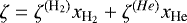 , where
  and
and  are the factional abundances of H2 and He, respectively. We calculate
  and xHe from the solar system abundance by Anders & Grevesse (1989):
 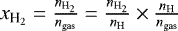 , with
  (all H nuclei are in the form of H2), and
 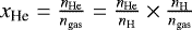 , with
  . Here, nH is the number density of hydrogen nucleus, which can be estimated as nH = ρgas∕(1.4mH) for the solarabundance (e.g., Igea & Glassgold 1999). In total, we have
 (10)
(10)
Besides, we followed standard prescriptions where the ionization rates are given as a function of vertical gas column densities:  and
and  , where
  and
and  represent the vertical gas column density measured from above and below a height of interest z, respectively, at a given radius r.
X-ray ionization rate  for H2
We adopt the fitting formula of Bai & Goodman (2009), based on the Monte Carlo simulations from Igea & Glassgold (1999). We estimate the total stellar X-ray luminosity LXR from the empirical median relationship LXR ≈ 10−3.5 × L⋆ (Güdel et al. 2007), and use the fitting coefficients at X-ray temperature TXR = 3 keV, which gives
 (11)
(11)
where
![Mathematical equation: \begin{multline*}\zeta^{(\textrm{H}_2)}_{{\textrm{XR},\,\textrm{direct}}}(r,z) = \left(\frac{L_{\textrm{XR}}}{10^{29} \, {\textrm{erg}\,\textrm{s}^{-1}}}\right) \left(\frac{r}{1 \, \textrm{au}}\right){}^{-2.2} \\\times\zeta_{\textrm{1,XR}} \left[\exp{\left(-\left(\frac{\Sigma_{\textrm{gas}}^{+}(r,z)}{\Sigma_{\textrm{1,XR}}}\right){}^{0.4} \right)} + \exp{\left(-\left(\frac{\Sigma_{\textrm{gas}}^{-}(r,z)}{\Sigma_{\textrm{1,XR}}}\right){}^{0.4} \right)} \right],\end{multline*}](/articles/aa/full_html/2022/02/aa41689-21/aa41689-21-eq37.png) (12)
(12)
and
![Mathematical equation: \begin{multline*}\zeta^{(\textrm{H}_2)}_{{\textrm{XR},\,\textrm{scattered}}}(r,z) = \left(\frac{L_{\textrm{XR}}}{10^{29} \, {\textrm{erg}\,\textrm{s}^{-1}}}\right) \left(\frac{r}{1 \, \textrm{au}}\right){}^{-2.2} \\\times \zeta_{\textrm{2,XR}} \left[\exp{\left(-\left(\frac{\Sigma_{\textrm{gas}}^{+}(r,z)}{\Sigma_{\textrm{2,XR}}}\right){}^{0.65} \right)} + \exp{\left(-\left(\frac{\Sigma_{\textrm{gas}}^{-}(r,z)}{\Sigma_{\textrm{2,XR}}}\right){}^{0.65} \right)} \right].\end{multline*}](/articles/aa/full_html/2022/02/aa41689-21/aa41689-21-eq38.png) (13)
(13)
The first term of Eq. (11) corresponds to the direct X-ray contribution of the total stellar X-ray ionization rate, whereas the second term corresponds to its scattered X-ray contribution.  describes attenuation of X-rays photons by absorption, with the unattenuated coefficient ζ1,XR = 6 × 10⁻¹² s−1 and the penetration depth Σ1,XR ≈ 0.0035 g cm−2.
  describes a contribution from scattering, with the unattenuated coefficient ζ2,XR = 10−15 s−1 and the penetration depth Σ2,XR ≈ 1.64 g cm−2. Here, we recalculated the penetration depths given by Bai & Goodman (2009) in terms of hydrogen nucleus into the corresponding gas surface density penetration depths (Σ1,XR and Σ2,XR).
Cosmic ray ionization rate  for H2
We adopt the following fitting formula given by Umebayashi & Nakano (2009):
![Mathematical equation: \begin{multline*}\zeta^{(\textrm{H}_2)}_{\textrm{CR}}(r,z) = \frac{\zeta_{\textrm{CR,ISM}}}{2} \\\times \Bigg\{\exp{\left(-\frac{\Sigma_{\textrm{gas}}^{+}(r,z)}{\Sigma_{\textrm{CR}}}\right)} \left[1+\left(\frac{\Sigma_{\textrm{gas}}^{+}(r,z)}{\Sigma_{\textrm{CR}}}\right){}^{\frac{3}{4}}\right]^{-\frac{4}{3}} \\ +\exp{\left(-\frac{\Sigma_{\textrm{gas}}^{-}(r,z)}{\Sigma_{\textrm{CR}}}\right)} \left[1+\left(\frac{\Sigma_{\textrm{gas}}^{-}(r,z)}{\Sigma_{\textrm{CR}}}\right){}^{\frac{3}{4}}\right]^{-\frac{4}{3}} \Bigg\},\end{multline*}](/articles/aa/full_html/2022/02/aa41689-21/aa41689-21-eq42.png) (14)
(14)
where we chose the unattenuated cosmic ray ionization rate ζCR,ISM = 10−17 s−1 and the cosmic ray penetration depth ΣCR = 96 g cm−2. Nevertheless, we note that the galactic cosmic ray ionization rate suffers from large uncertainties (e.g., McCall et al. 2003; Cleeves et al. 2013a).
Radionuclides ionization rate  for H2
The combined effect of the decay of short- and long-lived radionuclides is included in the following ionization rate
 (15)
(15)
where ζRA, 0 = 7.6 × 10⁻¹⁹ s−1. This constant is expected to be in the range (1 − 10) × 10−19 s−1, and is higher at smaller radii and early times (e.g., Umebayashi & Nakano 2009; Cleeves et al. 2013b). We further scaled the radionuclides ionization rate by the local dust-to-gas ratio ρdust∕ρgas, normalized by the ISM value 10−2. Since radionuclides (e.g., 26Al) are refractory and locked into dust particles, a change in the local dust-to-gas ratio is expected to induce a local change in the number of radionuclides locally available to ionize the gas. We note that Eq. (15) does not account for the escape of decay products, and therefore overestimates radionuclide ionization rates in low gas column density regions (Σgas ≲ 10 g cm−2). Nevertheless, radionuclide ionization does not dominate the total ionization rate in such regions of low gas surface densities reached in the outer disk regions. In practice, this inconsistency is thus not an issue.
We computed the ionization rate for H2 ζ(H2) by summing the X-ray, cosmic ray, and radionuclide contributions, as 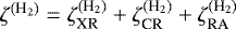 , and finally obtained the total ionization rate ζ (mean ionization rate for all gas molecules) using Eq. (10).
2.4 Ionization chemistry
By assuming that local ionization–recombination equilibrium is reached at every locations in the disk, we obtain the abundance of all charge carriers initiated by the ionization process. In this work, we do not implement a chemical reaction network (see, e.g., Bai & Goodman 2009; Semenov et al. 2004; Ilgner & Nelson 2006; Bai 2011). Instead, we implement a semi-analytical chemical model based on Okuzumi (2009). The main motivation behind our choice is the need of a chemical model that carefully captures the dust charge state as well as the gas ionization state, without greatly enhancing the computational complexity of the whole problem. The difference between the semi-analytical chemical model presented here and the one described in Okuzumi (2009) is the fact that we consider compact rather than fluffy grains.
Similar to Okuzumi (2009), the following fundamental approximations are made: (1) ions can be represented by a single dominant ion species; (2) the grain charge distribution can be approximated as a continuous function of Z. The key parameter in such an approach is the dimensionless parameter Γ that measures the ratio of the electrostatic attraction or repulsion energy between a charged dust particle and an incident ion or free electron, respectively, to the thermal kinetic energy. It is defined as
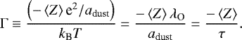 (16)
(16)
In the first equality,  is the meancharge carried by dust particles at a given location in the disk (r, z), and λO is given by
  ; with e the elementary charge, and T the gas temperature defined by Eq. (4). In the second equality, the dimensionless parameter τ is given by
  .
.
We need to further specify the forms of the effective collision cross-sections between ions/dust particles (σdi (Γ)) and free electrons/dust particles (σde(Γ)) to properly account for grain surface chemistry. Without loss of generality, they can be written as σdi (Γ) = siσdustPi(Γ) and σde (Γ) = seσdustPe(Γ), where  is the grain geometric cross-section; si = 1 and se = 0.3 are the sticking coefficients for ions and free electrons, respectively; Pi(Γ) and Pe(Γ) are dimensionless factors determined by the electrostatic interactions between ions/dust particles and free electrons/dust particles, respectively. Since we consider compact dust particles, we account for their induced electric polarization forces using the results from Draine & Sutin (1987). We assume
  (i.e., Γ > 0) because free electrons collide with grains much faster, hence more frequently than ions (see, e.g., Nishi et al. 1991; Wardle 2007). Consequently, Pi (Γ) and Pe (Γ) are functions of Γ that can be written as
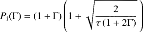 (17)
(17)
and
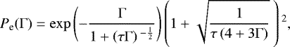 (18)
(18)
where Eqs. (17) and (18) are directly obtained from Eqs. (3.4) and (3.5) of Draine & Sutin (1987), respectively (see also Appendix A).
For a successful implementation of ionization chemistry in our disk model, we demand that charge neutrality is reached at every locations in the disk
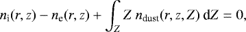 (19)
(19)
where ni is the total number density of ions, ne is the total number density of free electrons, and ndust(r, z, Z) is the number density of dust particles of net charge Z, located at (r, z).
For τ ≳ 1, the equilibrium grain charge distribution can be well approximated by a Gaussian distribution resulting in (Okuzumi 2009, see also Appendix A)
![Mathematical equation: \begin{equation*}n_{\textrm{dust}}(r,z,Z) = \frac{n_{\textrm{dust}}(r,z)}{\sqrt{2 \pi \left<\Delta Z^{2}\right>}} \exp{\left[-\frac{\left(Z - \left<Z\right> \right){}^{2}}{2 \left<\Delta Z^{2}\right>}\right]},\end{equation*}](/articles/aa/full_html/2022/02/aa41689-21/aa41689-21-eq55.png) (20)
(20)
where  is defined in Sect. 2.2, the mean grain charge
  is
is
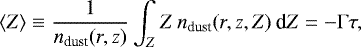 (21)
(21)
and the grain charge dispersion  is defined as
![Mathematical equation: \begin{equation*}\begin{split}\left(\sqrt{\left<\Delta Z^{2}\right>}\right){}^{2} &\equiv \frac{1}{n_{\rm{dust}}(r,z)} \int_{Z}^{} \left(Z-\left<Z\right>\right){}^{2} \: n_{\rm{dust}}(r,z,Z) \: \textrm{d}Z \\&= \left[\frac{1}{\tau} \left(\frac{d\ln{P_{\textrm{i}}(\Gamma)}}{\textrm{d} \Gamma} - \frac{d \ln{P_{\textrm{e}}(\Gamma)}}{d \Gamma} \right)\right]^{-1}\end{split}\end{equation*}](/articles/aa/full_html/2022/02/aa41689-21/aa41689-21-eq60.png) (22)
(22)
(see Appendix A for derivation of Eq. (22), and a complete expression).
Since the charge distribution is solely parametrized by Γ, ni and ne can be written as a function of that single parameter in the equilibrium state. Specifically, the balance between ionization and recombination yields (see Okuzumi 2009 and Appendix A)
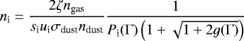 (23)
(23)
and
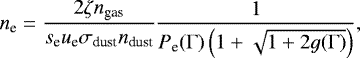 (24)
(24)
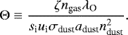
where
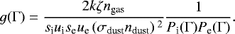 (25)
(25)
If g(Γ) ≳ 1 the recombination process is dominated by gas-phase recombination; otherwise, it is dominated by charge adsorption onto grains. k is the rate coefficient for the gas-phase recombination defined below, ζ is the total ionization rate determined by Eq. (10), ngas is the total number density of gas particles given in Sect. 2.2, and ui, ue are the mean thermal velocity of the dominant ion species and free electrons, respectively, given by 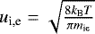 with mi being the mass of the dominant ion species. In this study, we assumed that the dominant ion species is HCO+ by setting mi = 29 mH and
 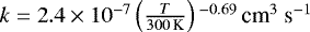 (see McElroy et al. 2013). The choice of the dominant ion species does not strongly affect our results as long as the dominant ions are molecular ions that recombine with free electrons dissociatively (e.g., Oppenheimer & Dalgarno 1974).
The only remaining unknown of the problem is the key parameter Γ. Equation (19) with Eqs. (21), (23), and (24) leads to the following equation whose root is Γ:
![Mathematical equation: \begin{equation*}\frac{1}{P_{\textrm{i}}(\Gamma)} - \left[\frac{s_{\textrm{i}} u_{\textrm{i}}}{s_{\textrm{e}} u_{\textrm{e}}} \frac{1}{P_{\textrm{e}}(\Gamma)} + \frac{\Gamma}{\Theta} \frac{\left(1 + \sqrt{1 + 2 g(\Gamma)}\right)}{2} \right] = 0,\end{equation*}](/articles/aa/full_html/2022/02/aa41689-21/aa41689-21-eq66.png) (26)
(26)
where Θ is a dimensionless parameter that quantifies which of the free electrons and dust particles are the dominant carriers of negative charge. It is defined by
 (27)
(27)
To summarize, the abundance of all charge carriers are written as analytical functions of the single key parameter Γ. By numerically solving Eq. (26), we obtain Γ and thus those abundances. In Appendix B, we compare our semi-analytical approach to a chemical reaction network.
3 Magnetorotational instability
The mass and angular momentum transport of weakly ionized protoplanetary disks is governed by MRI magnetic torques only if the coupling between the charged particles in the gas-phase and the magnetic field is sufficient; namely, the gas motion induced by those torques can generate magnetic stresses (due to orbital shear) faster than they can diffuse away due to nonideal MHD effects. In order to obtain the disk turbulence level encoded into the Shakura–Sunyaev α-parameter, we now need to know where the MRI can operate (Sect. 3.1), to choose an appropriate magnetic field strength (see Sect. 3.2), and to link the MRI stress to the disk turbulence state (Sect. 3.3).
3.1 Criteria for active MRI
In this study, the nonideal MHD effects considered are Ohmic resistivity and ambipolar diffusion. Their corresponding Elsasser numbers are defined as
 (28)
(28)
and
 (29)
(29)
where Λ is the Ohmic Elsasser number, ηO is the Ohmic magnetic diffusivity, Am is the ambipolar Elsasser number, ηAD is the ambipolar magnetic diffusivity, and vAz is the vertical component of the Alfvén velocity vA defined as 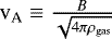 . We note the use of vA instead of vAz in Eq. (29), since we adopt the results of Bai & Stone (2011) who use vA to define Am. Here Bz is the vertical component of the magnetic field, and B is the strength of the r.m.s. field. We assume that those two quantities are related by
  (Sano et al. 2004). Our methodto constrain B is described in Sect. 3.2.
When Ohmic resistivity dominates, it has been shown that the MRI can be active if Λ > 1 (see, e.g., Sano & Stone 2002b; Turner et al. 2007). When ambipolar diffusion is the dominant nonideal MHD effect, and assuming the strong-coupling limit (see Appendix E.1), the MRI can operate even if Am < 1, provided that the magnetic field strength is “sufficiently weak” (Bai & Stone 2011). Here sufficiently weak means that the β-plasma parameter must exceed a minimum threshold βmin defined by Eq. (32).
Consequently, we consider the following set of conditions for sustaining active MRI:
 (30)
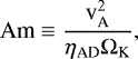
(30)
and
 (31)
(31)
The first condition will be referred in the following as the Ohmic condition, the second one as the ambipolar condition. Here the β-plasma parameter is defined as  . The minimum threshold βmin is a function of the ambipolar Elsasser number Am given by (Bai & Stone 2011)
 (32)
(32)
Whether the MRI is active or not depends on the magnetic diffusivities (ηO and ηAD), since they express the strength of their corresponding nonideal MHD effects. They are principally determined by the ionization degree of the gas as well as the magnetic field strength. Armed with the equilibrium abundances of all charge carriers computed in Sect. 2.4 and adopting the magnetic field strength obtained in Sect. 3.2, ηO and ηAD are computed at every locations of the protoplanetary disk by following Wardle (2007) (see their Eqs. (29) and (31)). To formally compute the various conductivities (σO, σH and σP from Wardle 2007), we need to specify for the momentum rate coefficient  (appearing in the coefficient γj of Wardle 2007, see their Eq. (21)) for ions (j ≡ i), free electrons (j ≡ e) and dust particles (j ≡dust). We adopt the formulation from Draine (2011) (see Table 2.1 and Eq. (2.34)), Bai (2011) (see Eq. (15)), and Wardle & Ng (1999) (see Eq. (21)); respectively for
  ,
,  , and
, and 
 (33)
(33)
![Mathematical equation: \begin{equation*}\left<\sigma v\right>_{\textrm{e}} = 8.3 \times 10^{-9} \times \max{\left[1,\sqrt{\frac{T}{100 \, \textrm{K}}} \:\right]} \, \textrm{cm}^{3}\,\textrm{s}^{-1}\end{equation*}](/articles/aa/full_html/2022/02/aa41689-21/aa41689-21-eq81.png) (34)
(34)
and
 (35)
(35)
where  is the reduced mass in a typical ion-neutral collision, T is the gas temperature defined by Eq. (4), and σdust is the grain geometric cross-section defined in Sect. 2.4.
An “MRI-active layer” is where both Eqs. (30) and (31) are satisfied; a “dead zone” is where the condition (30) is not met, so that Ohmic resistivity shuts off the MRI; and a “zombie zone” (as termed by Mohanty et al. 2013a) is where the condition (31) is not fulfilled, so that ambipolar diffusion prohibits the MRI-driven turbulence with too strong magnetic fields. With these conditions for active MRI, the underlying assumption is that the MRI is either in a saturation level allowed by the nonideal MHD effects or completely damped at any locations in the disk. Fundamentally, this assumption comes down to the fact that the MRI growth timescale is short (roughly  ) compared to viscous evolution timescales or dust evolution timescales.
The Hall effect has been ignored in the above criteria for active MRI, since quantifying its effect is beyond the scope of the present paper. Indeed, the inclusion of the Hall effect will further complicate the global picture, and it is still not clear how this nonideal MHD effect will impact the MRI when it dominates. As a result, we use the above conditions for the MRI even in the Hall-dominated regions of the protoplanetary disk. Nevertheless, we investigate where the Hall effect might be important and discuss the implications in Appendix E.2.
3.2 Magnetic field strength
The magnetic field strength plays a crucial role for the MRI since the magnetic diffusivities depend on it. In our study, we make the assumption that if the MRI can operate then: (1) the MRI activity is at the maximal efficiency as permitted by our conditions for active MRI; (2) the MRI-driven turbulence is in a saturation level allowed by the nonideal MHD effects; and (3) the magnetic field is constant with height across the MRI-active layer. Assumptions (2) and (3) are motivated by various 3D stratified and unstratified shearing box and global simulations. They show that the MRI saturates on a state permitted by the nonideal MHD effects (e.g., Hawley et al. 1995; Sano et al. 2004; Simon et al. 2011; Flock et al. 2012; Parkin & Bicknell 2013a,b); once saturated, turbulence stirring maintains the field strength roughly constant across the active layer (e.g., Miller & Stone 2000). Adopting assumption (1) implies that we opt for an optimistic view of the MRI activity, which will generate the highest accretion rate possibly reachable given the set of conditions for active MRI.
Assumption (1) is fulfilled by constraining and adopting the magnetic field strength so that it corresponds to the strongest field possible that would still allow for the MRI to operate (i.e., we want β-plasma as low as possible while satisfying both Eqs. (30) and (31)). In practice, we do so by maximizing the component of the steady-state accretion rate that comes from the MRI-active layer (Ṁacc, MRI). Using Eq. (24) of Bai (2011), it can be written as  , where hMRI is the MRI-active layer thickness. This formula is derived assuming that α ∝β−1 (see Sect. 3.3). Here we thus need to maximize the quantity hMRIB2, where we want B as strong as possibly allowed for the MRI to still operate. We note that hMRI implicitly depends on B, hence maximizing B alone formally leads to an infinitesimal hMRI, implying Ṁacc, MRI → 0. Indeed, ambipolar diffusion prohibits the MRI-driven turbulence with too strong magnetic fields as indicated by Eqs. (31) and (32).
Additionally, the MRI activity can be considered at maximal efficiency only if the most unstable modes (fastest growing modes) can develop in the MRI-active layer. In the upper layers of the MRI-active layer, the MRI behavior is marginally close to its ideal-MHD limit (Am ≈1; see Fig. F.1a). In this context, the wavelengths of the must unstable modes are given by (e.g., Sano & Miyama 1999)
 (36)
(36)
where vAz is the vertical component of the Alfvén velocity defined in Sect. 3.1. Assumption (1) ultimately comes down to the condition that the longest wavelength of the most unstable modes in the MRI-active layer must fit within both the disk gas scale height and the MRI-active layer thickness. Mathematically, this condition can be written as
 (37)
(37)
where  is the longest wavelength of the most unstable modes in the MRI-active layer, at any radii r. To summarize, the magnetic field strength B is chosen such that the MRI can operate (both Eqs. (30) and (31) must be satisfied) and the MRI is at maximal efficiency (we find B such that the quantity hMRIB2 is maximized, and the condition (37) is fulfilled).
To compute the magnetic field strength, we adopt a similar procedure as described in Mohanty et al. (2013a). For a specified disk radius r, we looped through a range of field strengths ![Mathematical equation: $B \in \left[10^{-5}-10^{3}\right] \,$](/articles/aa/full_html/2022/02/aa41689-21/aa41689-21-eq89.png) Gauss, which covers the plausible range in stellar accretion disks. For a given value of that range, we determined the MRI-active layer thickness hMRI. We then checked that the longest wavelength of the most unstable modes in the MRI-active layer fits within both the disk gas scale height and the MRI-active layer thickness. If it does, we computed the quantity hMRIB2. If not, we automatically discarded this magnetic field strength value by setting the quantity hMRIB2 to 0. We then reiterated the previous steps for the different field strength values in the range, and finally chose the final value B for this specific disk radius r such that the quantity hMRIB2 is the highest. We repeated the above steps for a range of radii
Gauss, which covers the plausible range in stellar accretion disks. For a given value of that range, we determined the MRI-active layer thickness hMRI. We then checked that the longest wavelength of the most unstable modes in the MRI-active layer fits within both the disk gas scale height and the MRI-active layer thickness. If it does, we computed the quantity hMRIB2. If not, we automatically discarded this magnetic field strength value by setting the quantity hMRIB2 to 0. We then reiterated the previous steps for the different field strength values in the range, and finally chose the final value B for this specific disk radius r such that the quantity hMRIB2 is the highest. We repeated the above steps for a range of radii ![Mathematical equation: $r \in \left[r_{\textrm{min}}-r_{\textrm{max}}\right]$](/articles/aa/full_html/2022/02/aa41689-21/aa41689-21-eq90.png) , until we obtained B as a function of disk radius r. Using this numerical radial profile, we finally reconstructed B in the vertical direction by further assuming that it is vertically constant.
, until we obtained B as a function of disk radius r. Using this numerical radial profile, we finally reconstructed B in the vertical direction by further assuming that it is vertically constant.
3.3 From the MRI accretion formulation to turbulence
The last key ingredient missing in our disk model is the link between accretion stress produced by either the MRI or hydrodynamic instabilities and the effective turbulent parameter  that goes into the Shakura–Sunyaev α-disk model. In particular, we must specify the local turbulent parameter α as a function of location in the disk (see Eq. (6)).
In non-MRI regions (dead or zombie zone), the source of viscosity is thought to be mainly from hydrodynamic instabilities that can produce non-MRI stresses. Since we did not run any hydrodynamic simulations, we assume the turbulence in all non-MRI regions to be encoded into a single constant turbulent parameter, αhydro. We further assume the hydrodynamic turbulent parameter, αhydro, to be constant across a given non-MRI zone regardless of whether the region is a dead or zombie zone. Motivated by the results from 3D global hydrodynamic simulations of the VSI (e.g., Flock et al. 2020; Barraza-Alfaro et al. 2021), we fiducially chose αhydro = 10−4.
In the regions of the disk where the MRI can operate (following our criteria in Sect. 3.1), a variety of numerical simulations show that there exists a tight correlation between the normalized accretion stress and the β-plasma parameter (see, e.g., Hawley et al. 1995; Sano et al. 2004; Pessah 2010; Bai & Stone 2011). The correlation can be represented by (see, e.g., Mohanty et al. 2018, their discussion in Appendix B)
 (38)
(38)
where β is the β-plasma parameter defined in Sect. 3.1, corresponding to the optimal r.m.s. magnetic field strength obtained by the method described in Sect. 3.2, and Wrϕ,MRI corresponds to the normalized accretion stress in the MRI-active layer. Here the total normalized accretion stress Wrϕ is defined as the sum of the Reynolds and Maxwell stresses normalized by the gas pressure.
In the MRI-active layer, we connect the local turbulent parameter αMRI to the normalized accretion stress Wrϕ,MRI by
 (39)
(39)
The factor “2/3” in Eq. (39) is explained in Sect. 2.2 of Hasegawa et al. (2017) and in Appendix B of Mohanty et al. (2018). Also, we added up the floor value αhydro because the MRI stress must dominate over the residual hydrodynamic stresses in MRI-active regions. If not, such regions are considered as dead in the sense that the turbulence is driven by hydrodynamic instabilities (even though the set of conditions for active MRI is satisfied).
To summarize, we calculate the appropriate effective turbulent parameter  (Eq. (6)) by specifying the local turbulent parameter α at all locations of the protoplanetary disk:
 (40)
(40)
where αDZ(r, z) = αAD(r, z) = αhydro, and αMRI(r, z) is given by Eq. (39).
4 Application: steady-state accretion
4.1 Approach
In this study, we apply our 1+1D global MRI-driven disk accretion model (described in Sects. 2 and 3) to investigate the steady-state MRI-driven accretion regime of a fiducial disk around a solar-type star. To do so, we self-consistently solved for the gas surface density through an iterative process (see Sect. 4.2), alongside the appropriate effective turbulent parameter  , to ensure the accretion rate Ṁacc to be radially constant (required for steady-state accretion) in the outer regions of the disk (r ≳ 1 au). In practice, for each step of the iteration process, we solved the coupled set of equations for both the gas surface density and the MRI. These equations are coupled because: (1)
  and Ṁacc are constrained by the MRI accretion, which depends on the disk structure; (2) the disk structure in steady-state accretion is determined by
  , Ṁacc, and stellar parameters. Although the detailed procedure is different, we note that our overall methodology is similar to the one adopted in Mohanty et al. (2018). The authors focus on regions around the dead zone inner edge (r < 1 au) by presenting a semi-analytical steady-state dust-free model in which the disk structure, thermal ionization and the viscosity due to the MRI are determined self-consistently. Among the key differences, our numerical model focuses on regions beyond 1 au (including the dead zone outer edge), include the relevant nonthermal ionization sources at those locations in the disk, and employ a semi-analytical chemical model to capture the charge state of the disk dust-gas mixture.
In our disk model, we chose Mdisk as a free input parameter and self-consistently obtained the corresponding Ṁacc, rather than choosing Ṁacc as the free parameter. This choice is particularly interesting if one wants to input the total disk gas mass. For example, this is useful for comparing the effective turbulent parameter  obtained for a steady-state accretion disk with a disk that would be out of equilibrium but with the same total disk gas mass; or if one wants to compare the equilibrium solutions obtained for different stellar masses, where the total disk gas mass is fixed. We note that setting either Ṁacc or Mdisk as the free input parameter of the model is equivalent and lead to the same results.
While the steady-state solution describes the inner inward-accreting region (r ≲ Rt) of viscously evolving disks well, it cannot treat the outer viscously expanding region (r ≳ Rt). Here Rt corresponds to the transition radius at which the gas motion changes from inward to outward in a viscously evolving disk (e.g., Hartmann et al. 1998). Ignoring this outer region, our steady model underestimates the real total disk gas mass. However, if we regard the outer boundary rmax of our disk model as the transition radius Rt, the neglected mass is at worst comparable to the mass within the model2.
4.2 The equilibrium solution
In the classical 1D viscous disk model, the steady-state accretion rate can be written as (for a derivation, see, e.g., Mohanty et al. 2018, their Appendix B):
 (41)
(41)
where  comes from the thin boundary-layer condition at the inner edge of the disk, assuming a zero-torque inner boundary condition (e.g., Armitage 2019). In the α-disk model, Rin is by definition the location where the Keplerian angular velocity ΩK plateaus and turns over. For instance, if the disk extends up to the stellar surface, Rin= R⋆ with R⋆ the stellar radius. In any case Rin ≪ 1 au, justifying the second equality in Eq. (41) that we shall use in this paper, since we study the structure of the outer disk (r ≳ 1 au).
Solving for Σgas by rearranging Eq. (41), we obtain the self-consistent steady-state gas surface density under the framework of viscously driven accretion
 (42)
(42)
When multiplying Eq. (42) by 2πr, integrating over radius and using the fact that Ṁacc is radially constant for steady-state accretion, we can find the relation between the accretion rate and the total disk gas mass Mdisk
 (43)
(43)
where rmin and rmax are the inner and outer boundary of our radial grid, respectively. Eq. (43) is another way of expressing the dependence of the accretion rate on the disk structure. It allows us to compute Ṁacc accordingly to the chosen free input parameter Mdisk, and ensure that the calculated Σgas is such that  . Here we emphasize that the total disk gas mass Mdisk is defined as the gas mass enclosed between rmin and rmax, and does not account for the mass residing beyond the outer boundary rmax (Mdisk is equal to the real total disk gas mass within a factor of two; see Sect. 4.1). Once the free input parameter Mdisk is chosen, we always compute Ṁacc using Eq. (43) and Σgas using Eq. (42), if not stated otherwise.
The steady-state Σgas and  are obtained by iterating through the following steps (those two quantities utterly determine the equilibrium solution in our disk model): Step 1 – compute the accretion rate Ṁacc (Eq. (43)) for a given fixed total disk gas mass, Mdisk; Step 2 – derive the steady-state gas structure by computing the gas surface density, Σgas (Eq. (42)), and reconstructing the gas volume density distribution, ρgas, under the hydrostatic equilibrium assumption; Step 3 - compute the total ionization rate, ζ, as in Sect. 2.3; Step 4 - derive the number densities of free electrons, ions, and charged dust particles by using the semi-analytical chemical model described in Sect. 2.4; Step 5 – derive the Ohmic and ambipolar magnetic diffusivities (ηO and ηAD) and obtain their corresponding Elsasser numbers from which a set of conditions for active MRI can be derived as in Sect. 3.1; and Step 6 – derive the local turbulent parameter α by connecting the MRI formulation of accretion to the α-disk model (Eq. (40)) and compute the effective turbulent parameter
  (Eq. (6)). After each Step 6, we checked that Σgas and
  are such that the right-hand side of Eq. (41) is radially constant, equal to the Ṁacc given by Eq. (43), at any disk radius. If not, we kept on iterating from Step 1 to Step 6 with the updated Σgas and
  from the previous iteration. The equilibrium solution is reached once the three following convergence conditions are met for the last 15 consecutive iterations: (1) Ṁacc is constant from iteration i-1 to iteration i within a 5% error; (2) the right-hand side of Eq. (41) is radially constant and equal to Ṁacc within a 5% error; and (3) Σgas is constant from iteration i − 1 to iteration i within a 5% error.
Our code converges toward a solution for the following reason. For a given fixed total disk gas mass, gas temperature profile, and stellar parameters, Ṁacc varies from iteration i-1 to iteration i only if  varies (see Eq. (43)). Once
  is constant from iteration i-1 to iteration i, Ṁacc becomes constant as well, and so does Σgas (Eq. (42)). In this study, we constrained and chose the r.m.s. magnetic field strength B such that the MRI activity is at the maximal efficiency as permitted by the nonideal MHD effects considered (see Sect. 3.2). Consequently,
  converges through iterations for the steady-state accretion solution to satisfy this condition.
We initially assumed that the protoplanetary disk is fully turbulent, and arbitrarily set  to be radially constant and equal to
 (in order to obtain the first Ṁacc and Σgas, required to initiate the iteration process). We checked that this choice does not affect the equilibrium solutions found.
5 Results: fiducial model
Applying our MRI-driven disk accretion model to describe the steady-state regime, we can now investigate the outer region structure (r ≳ 1 au) of steadily viscously accreting protoplanetary disks. We first present a detailed description of the equilibrium solution obtained using the method described in Sect. 4, for the fiducial model (M⋆ = 1 M⊙, L⋆ = 2 L⊙, Mdisk = 0.05 M⋆, adust = 1 μm, fdg = 10−2, αhydro = 10−4): the different accretion layers (Sect. 5.1); the disk structure (Sect. 5.2); and the disk turbulence level (Sect. 5.3). We then present the equilibrium solutions arising from variations in some of our fiducial parameters in Sect. 6.
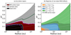 |
Fig. 1 Panel a: steady-state accretion layers, as a function of location in the disk, for the fiducial model. The black colored area corresponds to the dead zone. The gray colored area corresponds to the zombie zone. The red and black hatched area corresponds to the MRI-active layer. The region within the dash-dotted magenta lines defines where the ambipolar condition (β > βmin) is satisfied in the disk, while the region above the dashed cyan line defines where the Ohmic condition (Λ > 1) is fulfilled. The region above the solid green line corresponds to where β > 1. The dashed white lines correspond to the surfaces z = 1 Hgas, z = 2 Hgas, z = 3 Hgas, and z = 4 Hgas, from bottom to top, respectively. Panel b: Regimes of the nonideal MHD effects by showing the dominant magnetic diffusivities as a function of location in the disk. In the orange colored region the Ohmic resistivity dominates (ηO is the highest magnetic diffusivity), in the gray and blue colored regions the Hall effect dominates (|ηH | is the highest magnetic diffusivity), and in the green colored regions ambipolar diffusion dominates (ηAD is the highest magnetic diffusivity). The MRI-active layer is shown by the black hatched area. The dashed white lines are the same as in panel a. |
5.1 MRI-active layer, dead zone, and zombie zone
When Ohmic resistivity and ambipolar diffusion are the only nonideal MHD effects considered, the MRI-active layer is sandwiched between two inactive regions: the dead and the zombie zone.
Figure 1a shows the stratification of the disk with the three different accretion layers. First, we notice that the dead zone sits in the innermost regions where the gas density is the highest, whereas the zombie zone is located in the disk atmosphere where the gas density is low. Second, the MRI-active layer only develops in the upper layers for r ≲ 23 au, whereas the MRI operates from the mid-plane for r ≳ 23 au. As we see in Sect. 5.2.2, the ionization level is high enough only in the upper layers sitting right above the dead zone so that the MRI can only develop in a thin layer for r ≲ 23 au; until ambipolar diffusion prohibits it in the very upper layers. Conversely, for r ≳ 23 au, the ionization level is high enough right from the mid-plane so that the magnetic field can efficiently couple to the charged particles in the gas-phase to trigger the MRI. Third, in Fig. 1a, the region in between the dash-dotted magenta lines defines where the ambipolar condition (β > βmin) is satisfied in the disk, whereas the region above the dashed cyan line defines where the Ohmic condition (Λ > 1) is fulfilled. We note that: (1) the upper envelope of the MRI-active layer is utterly set by the ambipolar condition; (2) its lower envelope is mainly determined by the Ohmic condition (although the ambipolar condition plays a role for 2 au ≲ r ≲ 9 au). The latter result is different from previous studies (e.g., Mohanty et al. 2013a), where they find that both the upper and lower envelope of the MRI-active layer are completely set by the ambipolar condition around a Sun-like star. We can explain this difference as follows: First, they did not describe the steady-state accretion solution, resulting in a disk structure different from what is presented here. Second and most importantly, they used the total Alfvén velocity in their Ohmic condition, whereas we used its vertical component. Since the vertical component is five times less than the total quantity in our model ( ), our Ohmic Elsasser number is lower, resulting in a more stringent Ohmic condition in our study, and thus a more extended dead zone (both radially and vertically).
Figure 1b shows which one of the nonideal MHD effects dominates the magnetic diffusivities in the disk. The MRI-active layer is overplotted and shown by the black hatched area. We notice that ambipolar diffusion dominates in most regions of the protoplanetary disk (especially the zombie zone), followed by the Hall effect, and finally the Ohmic resistivity. As expected, ambipolar diffusion dominates the low-density regions such as the upper layers or the outermost regions (mid-plane included), Ohmic resistivity dominates the innermost and densest regions, and the Hall effect comes into play for intermediate regions. Furthermore, most of the MRI-active layer sits in the ambipolar-dominated region of the disk, implying that the MRI can be sustained there but it is weakened compared to its ideal limit (0.1 ≲ Am ≲ 10 in the MRI-active layer, as shown in Fig. F.1a). Particularly, the upper envelope of the MRI-active layer sits well within the region where the ambipolar magnetic diffusivity dominates; confirming that ambipolar diffusion sets it as seen above. On the other hand, Ohmic resistivity does not dominate the magnetic diffusivities where the lower envelope for the MRI-active layer sits. This result seems different from what we saw above, where we found that mainly Ohmic resistivity is important to determine the lower envelope of the MRI-active layer. This shows that Ohmic resistivity is the most stringent nonideal MHD effect to overcome for the MRI to operate, and does not need to dominate the magnetic diffusivities to have a strong impact on it.
Finally, it is quite striking that the Hall effect dominates the magnetic diffusivities in most of the dead zone as well as the inner regions of the MRI-active layer. Particularly, Figure 1b shows that the lower envelope of the MRI-active layer sits in the Hall-dominated region. We further discuss the implications in Appendix E.2.
5.2 Disk structure
5.2.1 Gas
The gas surface density is self-consistently derived -alongside the effective turbulence  - to ensure steady-state accretion (Eq. (42)). Figure 2 shows the steady-state radial profile (dotted red line) obtained through iterations.
It can be divided into two regions: a high-density region for r ≲ 23 au (mid-plane dead zone), and a low-density region for r ≳ 23 au (mid-plane MRI-active layer), where r = 23 au corresponds to the mid-plane dead zone outer edge. We note that the transition at the dead zone outer edge is sharp, and appears as a discontinuity. As we see in Sect. 5.3, the effective turbulent parameter  sharply increases by jumping from a low turbulence state in the non-MRI regions to a high turbulence state in the MRI-active layer at r = 23 au. Since the accretion rate must be kept radially constant to ensure steady-state accretion, the gas surface density compensates by sharply decreasing at that location.
The profile displayed in Fig. 2 is actually expected. Indeed, if one initially assumes the disk to be out of equilibrium with its gas surface density following, for example, the self-similar solution from Lynden-Bell & Pringle (1974), the accretion rate will be radially variable, where the outer regions (MRI-active layer) accrete more than the inner ones (dead zone) on average. Consequently, by letting viscously evolving the gas, one will find that the gas is depleted from the MRI-active layer to be accumulated into the dead zone.
5.2.2 Ionization level
Since the gas content is mostly located within the dead zone, the ionization level is highly heterogeneous across the protoplanetary disk. Figures 3 and 4 show the steady-state total ionization rates for H2 for the differentnonthermal ionization sources considered (stellar X-rays, galactic cosmic rays, radionuclides) and the steady-state ionization fraction (free electron abundance), respectively.
Deep inside the dead zone (r ≲ 5 au and z ≲ 1.5 Hgas), the ionization solely comes from the decay of short- and long-lived radionuclides (Figs. 3a and 3b). In those innermost regions, the gas surface density is so high that the other nonthermal ionization sources cannot penetrate at all, resulting in a very low ionization fraction (Fig. 4a). For 9 au ≲ r ≲ 23 au and z ≲ 1.5 Hgas, galactic cosmic rays can penetrate deep enough to dominate the ionization process, leading to an increase in the ionization fraction (Figs. 4a and 4b). Right at the mid-plane dead zone outer edge (r = 23 au), the gas becomes tenuous enough for scattered stellar X-rays to come into play and contribute as much as the galactic cosmic rays (Fig. 3a). As a result, the total ionization rate for H2 gets a ”boost” at the transition between the mid-plane dead zone and the mid-plane MRI-active layer (comparing the black solid curves in Figs. 3c and 3d). We further notice that stellar X-rays (both the scattered and direct contributions) can overall penetrate deeper for r ≳ 23 au due to lower gas column densities. Consequently, the ionization fraction sharply increases at the transition between themid-plane dead zone and the mid-plane MRI-active layer (comparing the red and blue curves of Fig. 4b), resulting in enough charged particles in the gas-phase for the magnetic field to couple with and triggering the MRI from the mid-plane (not only in the surface layers as it is the case for r ≲ 23 au). Although the total ionization rate for H2 is utterly dominated by stellar X-rays in the disk atmosphere (either through the scattered or direct contribution), Fig. 3a shows that galactic comic rays always dominate at the mid-plane for r ≳ 23 au. This behavior can be understood as follows: On one hand, the total stellar X-ray ionization rate (sum of the scattered and direct contribution) decreases over radius (∝ r−2.2) unlike the ionization rate from galactic cosmic rays. Even though the gas is tenuous enough for the stellar scattered X-rays to penetrate deep enough, this emission has already lost most of its energy by traveling up to those regions. On the other hand, the stellar direct X-rays have a very small penetration depth -although they are the most energetic source of ionization considered here. The gas is thus not tenuous enough for them to efficiently ionize the mid-plane. Interestingly, we notice that the total ionization rate for H2 roughly saturates at a value equal to ζ(H2) ≈ 1.5 × 10⁻¹⁷ s−1 in the mid-plane MRI-active layer (Fig. 3a): the galactic cosmic ray ionization rate saturates at its unattenuated value 10−17 s−1, and the total stellar X-ray ionization rate roughly adds up 0.5 × 10⁻¹⁷ s−1). Consequently, the ionization fraction monotonously increases in the mid-plane MRI-active layer (Fig. 4a).
Finally, we use the fit from Bai & Goodman (2009) to compute the stellar X-ray ionization rate. Since the gas content is mostly located in the inner regions of the protoplanetary disk, the inner regions might absorb stellar direct X-rays before they could actually reach the outer regions. This self-shadowing event could thus prevent stellar X-rays from efficiently ionizing the outer regions of the protoplanetary disk, resulting in an overall lower ionization level. We further discuss this point in Appendix C.
In summary, we find that (see Fig. C.1): (1) the decay of short- and long-lived radionuclides dominates the ionization process in the innermost regions of the dead zone; (2) galactic cosmic rays dominate the outermost regions of the dead zone, the whole mid-plane MRI-active layer, and most of the regions right about the mid-plane MRI-active layer; (3) stellar scattered X-rays dominate the lower layers of the disk atmosphere that sit right above the dead zone, and contribute as much as galactic cosmic rays right at the mid-plane dead zone outer edge; (4) stellar direct X-rays dominate the ionization process in the upper layers of the disk atmosphere, including the lower layers of the outermost regions; (5) the MRI is mainly driven by stellar X-rays, except close to the mid-plane where it is primarily driven by galactic cosmic rays.
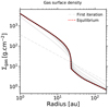 |
Fig. 2 Steady-state gas surface density, Σgas (Eq. (42)), as a function of radius, for the fiducial model. The dashed gray line shows the initial gas surface density by initially assuming that the effective turbulent parameter,
|


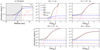 |
Fig. 3 Steady-state ionization rates for the fiducial model. The total ionization rate for H2 (ζ(H2); solid black line) is the sum of the following contributions: the radionuclides ionization rate for H2 ( |


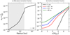 |
Fig. 4 Steady-state ionization fraction, xe (ne is defined by Eq. (24)), for the fiducial model. Panel a: mid-plane ionization fraction as a function of radius. The gray shaded area corresponds to the radial locations within the mid-plane dead zone. Panel b: vertical profiles for the ionization fraction at the same radial locations as in Fig. 3. The solid black line corresponds to r = 1 au. The solid red line corresponds to r = 23− au. The solid blue line corresponds to r = 23+ au. The solid green line corresponds to r = 80 au. |
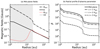 |
Fig. 5 Steady-state quantities describing the disk magnetization for the fiducial model. Panel a: mid-plane magnetic fields strength as a function of radius. The solid black line corresponds to B, the optimalr.m.s. magnetic field strength that is required for the MRI activity to be at the maximal efficiency as permitted by Ohmic resistivity and ambipolar diffusion (Sect. 3.2). The dotted red line corresponds to
|
5.2.3 Magnetic field strength
A lower limit on the magnetic field strength is the mean galactic field, which is roughly equal to 10−5 G (e.g., Beck & Hoernes 1996), whereas an upper limit is the equipartition field (field such that the gas thermal pressure and the magnetic pressure are equal), which makes the shortest unstable MRI mode no longer fit within the disk gas scale height (hence, no MRI activity possible at all). In this study, we numerically constrained the magnetic field strength, B, such that the MRI activity is at the maximal efficiency as permitted by Ohmic resistivity and ambipolar diffusion at any locations in the disk.
Figure 5a shows the various mid-plane fields of interest as a function of distance from the star. As expected, the highest value for B is well below the equipartition field  , while its lowest value is well above the mean galactic field. We notice that the optimal r.m.s. magnetic field B displays a small discontinuity located at the mid-plane dead zone outer edge (r = 23 au). Although nonphysical, this mathematical discontinuity expresses the fact that B jumps from a solution in the dead zone where the turbulence is weak to another in the MRI-active layer where the turbulence is stronger. In the mid-plane MRI layer (r ≳ 23 au), B is very close (but strictly lower) to
  , which corresponds to the maximal field strength from and above which the MRI-driven turbulence with such a field strength is prohibited by ambipolar diffusion (see Eqs. (31) and (32)). This is expected since we constructed the field strength such that the MRI operates at maximal efficiency. We further notice that the optimal r.m.s. magnetic field B is higher than Bmax for r ≲ 18 au. It thus implies that the ambipolar condition is also not met in most of the mid-plane dead zone where the MRI is suppressed by Ohmic resistivity, as we saw in Sect. 5.1
Figure 5b shows the β-plasma parameter radial profiles at various heights in the disk. Since the optimal r.m.s. magnetic field B is assumed to be vertically constant, β-plasma decreases exponentially with increasing height; hence, the radial profiles at different disk gas scale height are rescaled versions of the mid-plane profile (solid line). In the mid-plane dead zone (r ≲ 23 au), the mid-plane β-plasma parameter has a mean value of roughly 8 × 10³. As expected, the mid-plane dead zone is thus weakly magnetized, since the MRI cannot operate. In the mid-plane MRI-active layer (r ≳ 23 au), the mid-plane β-plasma parameter has a mean value of roughly 142, implying that these regions are moderately magnetized. We further notice that the mid-plane β-plasma saturates in the MRI-active layer from r ≳ 60 au. This behavior can be understood as follows: As seen in the last section, the mid-plane ionization fraction increases with radius (Fig. 4a); this results in the magnetic field being more efficiently couple to the gas in these regions, which leads to a possible stronger MRI-driven local turbulence. However, ambipolar diffusion is the dominant nonideal MHD effect in the regions where the gas is scarce, as we saw in Sect. 5.1. In such regions, a stronger local MRI-driven turbulence implies a stronger field strength (α ∝ β−1), resulting in this stronger local turbulence being prohibited by ambipolar diffusion. Consequently, the mid-plane β-plasma parameter saturating in the MRI-active layer from r ≳ 60 au expresses that the positive feedback on the MRI from a higher gas ionization degree is compensated for by the negative feedback from ambipolar diffusion that prohibits turbulence with stronger magnetic fields.
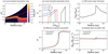 |
Fig. 6 Steady-state quantities describing the turbulence state in the disk for the fiducial model. Panel a: local turbulence parameter, α (Eq. (40)), as a function of location in the disk. The region above the solid red line corresponds to where β > 1. The dashed white lines correspond to the surfaces z = 1 Hgas, z = 2 Hgas, z = 3 Hgas, and z = 4 Hgas, from bottom to top, respectively. Panel b: vertical profiles for the local turbulent parameter, α, at various radial locations, with color codes as in Fig. 4. Panel c: MRI-active layer thickness, hMRI, as a function of radius, expressed in terms of the disk gas scale height, Hgas. Panel d: pressure-weighted vertically integrated turbulent parameter, |

5.3 Turbulence
In this study, the origin of turbulence is the radial transport of angular momentum redistributed within the protoplanetary disk by standard viscous torques: MRI magnetic torques in the active regions, and hydrodynamic torques in the non-active regions. Figure 6 shows various quantities of interest describing the properties of the steady-state disk turbulence.
As expected, the disk is significantly more turbulent in the MRI-active layer than it is in the dead or zombie zone. From Figs. 6a and 6b, we notice that the local turbulent parameter α is higher at large radii and heights, in the MRI-active layer. Indeed, the ionization level is higher in these regions because the gas surface densities arelower, leading to more penetration by the nonthermal ionization sources (stellar X-rays in the disk atmosphere, and galactic cosmic rays at the disk mid-plane) as well as slower recombination. At the mid-plane dead zone outer edge (r = 23 au), the turbulence jumps from a low regime in the mid-plane dead zone to a high regime in the mid-plane MRI-active layer. More generally, this very steep transition happens at the boundaries between active and non-active regions; namely, at the upper and lower envelopes of the MRI-active layer. We obtain such a behavior due to our assumption on the MRI: either in a saturation level allowed by the nonideal MHD effects, or completely shut off (see criteria in Sect. 3.1). Figure 6d shows that, due to this sharp change, the effective turbulent parameter  displays a small discontinuity at the mid-plane dead zone outer edge (r = 23 au), resulting in the discontinuity seen in the steady-state gas surface density (Fig. 2). We further discuss such a sharp transition inthe gas surface density profile in Sect. 7.1.
Since there is a thin turbulent MRI-active layer that sits right above the dead zone for r ≲ 23 au, the effective turbulent parameter  is higher than the minimum value αhydro = 10−4 in the dead zone, and increases toward the dead zone outer edge (see dotted red line in Fig. 6d). If not located too high above the dead zone, active regions can indeed make the dead zone effectively more turbulent by launching turbulent waves (e.g., Fleming & Stone 2003; Oishi & Mac Low 2009; Dzyurkevich et al. 2010; Okuzumi & Hirose 2011). Although such waves are not described by our disk model, the effective turbulent parameter
  encodes the influence of the upper layers on the turbulence, since this quantity is the pressure-weighted vertical average of the local turbulence. In the innermost regions of the dead zone,
  because the MRI-active layer represents a very small fraction of the gas column densities. Since the vertical extent of the dead zone diminishes for larger radii, the active regions right above the dead zone increasingly represent a higher fraction of the gas column densities toward the dead zone outer edge; meaning that the contribution from the MRI-active layer on the effective turbulent parameter
  increasingly becomes larger. Overall, though, we find that the mean value of
  is roughly 1.7 × 10⁻⁴ in the dead zone. Therefore, the general behavior of the turbulence in these regions is a low regime, as expected.
Conversely, the dotted red line in Fig. 6d shows that the mean value of  in the outer region of the MRI-active layer (r ≳ 23 au) is roughly 3.1 × 10⁻³, which is 19 times higher than the mean value stated above for the dead zone. Interestingly, we notice that the effective turbulent parameter
  decreases for r ≳ 60 au. This seems to be at odds with the fact that the local turbulent parameter α saturates and is roughly constant for a given height at those radii (because α ∝ β−1 and β-plasma is roughly constant for a given height at those radii, as seen in Fig. 5b). To better understand this behavior, the MRI-active layer thickness hMRI is shown in Fig. 6c. We notice that it diminishes comparatively to Hgas for r ≳ 23 au. Indeed, hMRI increases toward larger radii, but slowly since local turbulence with stronger than permitted magnetic fields would be considered if the active layer was thicker at a given r, which is prohibited by ambipolar diffusion. As a result, the quantity hMRI∕Hgas slowly decreasing for r ≳ 23 au implying that the MRI-active layer increasingly represents a lower fraction of the gas column densities for increasing radii from r ≳ 23 au. For a local turbulent parameter α roughly constant for r ≳ 60 au and a reduction in how much the MRI-active layer contributes to the gas column densities, the effective turbulent parameter
  decreases for r ≳ 60 au.
In summary, we find that the effective turbulent parameter  is strong when both the local MRI-driven turbulence α and the MRI-active layer thickness hMRI (comparatively to Hgas) are significant: The former tells us how much turbulence can be locally driven by the MRI, whereas the latter describes how much the MRI-active layer contributes to the gas column density at a given radius.
We emphasize that the accretion rate Ṁacc presented inFig. 6e represents the highest value possibly reachable given the set of criteria for active MRI employed, since we adopt the required magnetic field strength such that the MRI activity is at maximal efficiency (see Sect. 3.2). In Appendix D.1, we explore what would be the derived accretion rates for either weaker or stronger magnetic field strengths, and show that our choice for the magnetic field strength leads to the highest value for the accretion rate as expected.
6 Results: parameter study
We performed a series of simulations exploring the effect of various model parameters on the fiducial model described in the last section: total disk gas mass Mdisk (Sect. 6.1), representative grain size adust (Sect. 6.2), vertically integrated dust-to-gas mass ratio fdg (Sect. 6.3), and stellar properties – mass M⋆ and luminosity L⋆ – (Sect. 6.4). In each series, we derived key quantities reached by our steady-state accretion disk model as a function of distance from the central star. These quantities are: (a) the pressure-weighted vertically integrated turbulent parameter  ; (b) the gas surface density Σgas; (c) the mid-plane total ionization rate ζ; (d) the mid-plane optimal r.m.s. magnetic field strength B required for the MRI activity to be at maximal efficiency; (e) the accretion rate Ṁacc; (f) the mid-plane location of the dead zone outer edge RDZ (corresponding to the dead zone maximal radial extent). A detailed description of the results are given in the following sections. In Appendix D, we additionally investigate the effect of magnetic field strength, hydrodynamic turbulent parameter αhydro, gas temperature model T(r), as well as the combined effect of stellar properties and total disk gas mass.
6.1 The effect of disk mass
The amount of gas enclosed within the protoplanetary disk sets many of the disk structure properties (e.g., ionization level). It is then expected that the variation in total disk gas mass will significantly impact the equilibrium solution. To quantify this further, we ran a set of simulations where Mdisk varies from a gas-poor disk motivated by the ALMA observations in the continuum (see, e.g., Pascucci et al. 2016, assuming a gas-to-dust ratio of 100) to a gas-rich disk close to the GI limit. Our disk model does not treat gravito-turbulence, and hence the GI limit sets the upper limit for the total disk gas mass. We determined such an upper limit by choosing a total disk gas mass value so that Q ≳ 2 is satisfied at every radii r, where Q is the Toomre parameter (Toomre 1964). In practice, we chose Mdisk in the list {0.005, 0.01, 0.05, 0.10} M⋆ with M⋆ = 1 M⊙. The results can be seen in Fig. 7.
As expected for a steady-state viscously accreting protoplanetary disk, the accretion rate and total disk gas mass follow a tight correlation (Fig. 7e). Particularly, we find that  . In our model,
  . Consequently, Eq. (43) gives:
For fixed L⋆ and M⋆, the quantity Ṁacc∕Mdisk is entirely determined by the integral  . We find that
 ![Mathematical equation: $\left[\int_{r_{\textrm{min}}}^{r_{\textrm{max}}}\bar{\alpha}^{-1}\textrm{d}r \right] \propto M^{0.46}_{\rm{disk}}$](/articles/aa/full_html/2022/02/aa41689-21/aa41689-21-eq134.png) , hence the relation between Ṁacc and RDZ. Physically, this relation can be simply understood as follows: a higher total disk gas mass implies more gas available to be accreted onto the central star, hence a higher accretion rate.
, hence the relation between Ṁacc and RDZ. Physically, this relation can be simply understood as follows: a higher total disk gas mass implies more gas available to be accreted onto the central star, hence a higher accretion rate.
Additionally, we find a similar correlation between the dead zone maximal radial extent and the total disk gas mass  . Figure 7f shows that the dead zone maximal radial extent (corresponding to the mid-plane dead zone outer edge) can be as small as ≈ 4 au for low total disk gas masses, and as large as ≈31 au for high total disk gas masses. For a massive disk, the gas surface density is higher at every radii; leading to a lower ionization state compared to a low total disk gas mass (Fig. 7c). Since the ionization fraction is lower, there are less charged particles in the gas-phase for the magnetic field to couple with. Consequently, the mid-plane dead zone outer edge is located further away because the location where the ionization level is enough to trigger the MRI is reached further away. With the same argument on the overall lower gas ionization degree, we can explain why the mean value of the overall effective turbulent parameter
  is lower for disks with a higher total disk gas mass.
Interestingly, we notice that  displays a different shape for the two less massive disks. Instead of only steeply increasing right at the dead zone outer edge, it also displays a second shallow but significant increase in the MRI-active layer. We can explain the shape displayed for the two less massive disks by looking at their mid-plane total ionization rate (Fig. 7c): for such low total disk gas masses, the ionization process (mid-plane included) is dominated by stellar X-rays. The scattered X-ray contribution dominates right at the dead zone outer edge (first steep increase in ζ) but quickly decreases for larger radii, while the direct X-ray contribution increases from the dead zone outer edge but cannot penetrate deep enough yet. As a result, the mid-plane total ionization rate immediately decreases beyond the dead zone outer edge, until the direct X-ray contribution can finally penetrate deep enough to compensate for the decrease in the scattered X-ray contribution and provide another boost to the mid-plane ionization (second shallow increase in ζ).
Furthermore, we find that the optimal r.m.s. magnetic field strength B is weaker for a lower total disk gas mass once the mid-plane MRI-active layer is reached due to ambipolar diffusion (Fig. 7d). Since a lower total disk gas mass implies a higher gas ionization degree at the mid-plane, the ambipolar Elsasser number Am is slightly higher once the mid-plane MRI-active layer is reached (for example, we find that Am can be up to three times higher for Mdisk = 0.005 M⋆ compared to Mdisk = 0.05 M⋆). This implies that βmin(Am) is slightly lower for a lower total disk gas mass in such regions (it can be up to four times lower for Mdisk = 0.005 M⋆ compared to Mdisk = 0.05 M⋆). However, the gas surface densities are much lower across the disk for a lower total disk gas mass, leading to an overall lower gas volume density ρgas (it is at best four times lower for Mdisk = 0.005 M⋆ compared toMdisk = 0.05 M⋆). Since the threshold for the magnetic field strength from and above which the MRI-driven turbulence with such a field strength is prohibited by ambipolar diffusion (Bmax) is such that  , and ρgas decreases faster than βmin(Am) does for a lower total disk gas mass, weconclude that Bmax is lower, hence a lower B.
Finally, a striking result is that the effective turbulence level roughly becomes independent of the total disk gas mass considered at r ≈ 200 au (all the  converge toward the same value ≈3 × 10⁻³). This shows how ambipolar diffusion operates as a regulator to compensate for the positive feedback on the MRI from a higher gas ionization degree for a lower total disk gas mass, as explained in the previous paragraph.
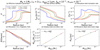 |
Fig. 7 Effect of the total disk gas mass on the equilibrium solution when varying the parameter Mdisk from 0.005 M⋆ (gas-poor disk) to 0.10 M⋆ (gas-rich disk close to the GI limit): The case Mdisk = 0.005 M⋆ is shown in blue, Mdisk = 0.01 M⋆ in dark orange, Mdisk = 0.05 M⋆ in green (fiducial model), and Mdisk = 0.10 M⋆ in red. The panels show the various steady-state profiles of some key quantities, for the model parameters M⋆ = 1 M⊙, L⋆ = 2 L⊙, adust =1 μm, fdg = 10−2, and αhydro = 10−4. Panel a: pressure-weighted vertically integrated turbulent parameter, |

6.2 The effect of grain size
The representative grain size at a given location in the disk is subject to significant change over time due to processes such as coagulation, fragmentation or radial drift. Depending on whether the representative grain size is skewed toward small or large dust particles, the equilibrium solution is expected to be very different. In our disk model, we do not yet account for dust evolution or multiple dust species. Nevertheless, we can still roughly quantify the importance of grain size on the equilibrium solution by running a set of simulations where we uniformly varied the dust particles size from submicron to millimeter. In practice, each dust particle has the same radius adust, with adust in the list {10−5, 10−4, 10−3, 10−2, 10−1} cm. The results can be seen in Fig. 8.
A smaller grain size implies a lower accretion rate and a more extended dead zone (Figs. 8e and 8f). Smaller dust particles have indeed higher cross-section areas allowing them to efficiently capture free electrons or ions (overall lower ionization level, Fig. 8c). Since there are less charged particles in the gas-phase for the magnetic field to couple with, the MRI cannot be triggered easily and can even be shut off in most of the disk by strong Ohmic resistivity and ambipolar diffusion. Particularly, for submicron grains and at the mid-plane, the MRI can develop in the outermost regions of the disk only (r ≳ 92 au, Fig. 8a). For r ≲ 92 au, the MRI can only operate in the surface layers, since the effect of grains on the ionization chemistry is diminished and stellar X-rays can more efficiently ionize the gas. Nonetheless, it is not enough to compensate for the fact that most of the disk is MRI-dead; leading to a mean value of a few times 10−4 for  . Overall the accretion rate is thus much lower for submicron grains.
For larger grain sizes, the overall ionization level in the disk becomes higher for two reasons: The cross-section is significantly reduced, resulting in the gas-phase recombination more easily dominating the recombination process, and dust settling becomes important. Regarding the latter, larger dust particles easily decouple from the gas in the upper layers of the disk atmosphere, where the turbulence level is low due to ambipolar diffusion (see Sect. 5.3). Consequently, settling can overcome vertical stirring, resulting in the dust being concentrated in regions closer to the mid-plane. Dust settling thus implies a higher local dust-to-gas ratio closer to the mid-plane, hence a higher mid-plane radionuclides ionization rate since the ionization from radionuclides is mainly due to 26Al locked into grains. The effect of dust settling can be seen in Fig. 8c, where the total mid-plane ionization rate is the highest for adust = 1 mm, for r ≲ 4 au.
Another salient result is that the steady-state accretion solution becomes independent of the grain size choice for adust ≳ 100 μm. We can thus infer that there exists a threshold for the grain size above which the grains have little impact on the ionization chemistry, hence on the ionization level, and ultimately on the MRI.
Finally, once the mid-plane MRI-active layer is reached, we notice that the corresponding mean value of  is roughly independent of the grain size, in the range 2 × 10⁻³–3 × 10⁻³ (Fig. 8a). We saw previously that the disk becomes more MRI-dead when smaller grain sizes are considered, implying that the gas surface densities in the MRI-active layer are lower compared to the ones for larger grain sizes (required to preserve the total disk gas mass constant). Since the gas surface densities are lower in the MRI-active layer for smaller grain sizes (Fig. 8b), we would expect more charged particles available in the gas-phase (due to stronger ionization) in such regions compared to the case of larger grain sizes. However, these charged particles are more efficiently captured when the dust grains are small, implying that the effective ionization level is actually not higher than the ones for larger grain sizes. Once the MRI-active layer is reached, its mean effective turbulence level is thus roughly constant regardless of the grain size.
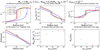 |
Fig. 8 Effect of the grain size on the equilibrium solution when varying the parameter adust from 0.1 μm to 1 mm: The case adust = 0.1 μm is shown in blue, adust = 1 μm in dark orange (fiducial model), adust = 10 μm in green, adust = 100 μm in red, and adust = 1 mm in purple. The panels show the various steady-state profiles of some key quantities, for the model parameters M⋆ = 1 M⊙, L⋆ = 2 L⊙, Mdisk = 0.05 M⋆, fdg = 10−2, and αhydro = 10−4. Panels a–f show the same key quantities as in Fig. 7. |
6.3 The effect of the dust-to-gas mass ratio
Whether small dust particles are depleted or accumulated is expected to be crucial for the equilibrium solution, since the higher the concentration of those is, the harder it is for the MRI to operate. We ran two sets of simulations where we: (1) consider an overall change in the vertically averaged dust-to-gas mass ratio from 10−5 (99.9% depletion of dust particles relative to standard ISM) to 10−1 (Sect. 6.3.1); (2) impose local dust enhancements either at the expected dead zone outer edge location for the fiducial model (r = 23 au) or at two locations in the disk, respectively, r = 5 au, which is within the mid-plane dead zone, and r = 60 au, which is within the mid-plane MRI-active layer (Sect. 6.3.2).
6.3.1 Overall change
For this set of simulations, the vertically averaged dust-to-gas mass ratio fdg is chosen to be radially constant and equal toa value in the list {10−5, 10−4, 10−3, 10−2, 10−1}. The results can be seen in Fig. 9.
Figures 9e and 9f show that protoplanetary disks with an overall higher depletion of micron-sized dust particles have a higher accretion rate and a more compact dead zone. For a disk poor in micron-sized grains, Ohmic resistivity and ambipolar diffusion are less stringent on the MRI activity because the amount of small grains is not enough to significantly impact the recombination process, happening then mostly in the gas-phase; although the overall ionization level in the innermost regions is lower compared to less depleted disks due to fewer radionuclides being available (Fig. 9c).
For a disk rich in micron-sized grains, the ionization from the decay of short- and long-lived radionuclides is stronger. However, it is not enough to compensate for the more stringent nonideal MHD effects on the MRI-driven turbulence, since a higher number of grains can more efficiently sweep up free electrons and ions from the gas-phase. Particularly, the case fdg = 10−1 leads to the lowest accretion rate (≈2 × 10⁻⁹ M⊙ yr−1) and the largest dead zone maximal radial extent (≈47 au).
We notice that the steady-state accretion solution becomes independent of the vertically averaged dust-to-gas mass ratio choice for fdg ≲ 10−4. Similarly to what we saw for the effect of grain size, there exists a threshold below which the dust depletion is so high that the grains barely have an impact on the ionization chemistry. Consequently, an even higher depletion would not change the ionization level, and ultimately the MRI.
Finally, the mean effective turbulence level is roughly independent of the vertically averaged dust-to-gas mass ratio once the MRI-active layer is reached (Fig. 9a). This can be explained by a similar argument used in the previous section: Although the gas surface densities in the MRI-active layer are lower for higher fdg (which is expected to result in more charged particles available in the gas-phase due to stronger ionization), these charged particles are more efficiently captured by the dust for higher fdg. It implies that the effective ionization level is actually not higher than the ones for lower fdg; hence, the mean effective turbulence level in the MRI-active layer is roughly constant regardless of fdg.
 |
Fig. 9 Effect of overall change in the vertically integrated dust-to-gas mass ratio on the equilibrium solution when varying the radially constant parameter fdg from 10−5 (99.9 dust depletion relative to standard ISM) to 10−1 (dust-rich disk): The case fdg = 10−5 is shown in blue, fdg = 10−4 in dark orange, fdg = 10−3 in green, fdg = 10−2 in red (fiducial model), and fdg = 10−1 in purple. The panels show the various steady-state profiles of some key quantities, for the model parameters M⋆ = 1 M⊙, L⋆ = 2 L⊙, Mdisk = 0.05 M⋆, adust =1 μm, and αhydro = 10−4. Panels a–f show the same key quantities as in Fig. 7. |
6.3.2 Local enhancements
In the first scenario, a fixed local dust enhancement (either moderate or strong) is imposed at the expected dead zone outer edge location for the fiducial model (r = 23 au). By doing so,we want to investigate how the equilibrium solution changes if dust particles have accumulated at the dead zone outer edge before the steady-state accretion regime is reached. In the second scenario, a fixed local dust enhancement (either moderate or strong) is imposed at either r = 5 au or r= 60 au. Here our goal is to study how local dust enhancements due to, for example, spontaneous traffic jams can impact the steady-state accretion solution if they occur before the steady-state accretion regime is reached. Such traffic jams can form at locations where the gas pressure is enhanced (without the gas pressure gradient to necessarily flip of sign). The results can be seen in Fig. 10.
For both scenarios, a moderate local dust enhancement refers to a local change in the vertically averaged dust-to-gas mass ratio from 10−2 to 5 × 10⁻² (referred as “5 × enhancement”), whereas a strong one refers to a local change from 10−2 to 10−1 (referred as “10 × enhancement”). Local dust enhancements are implemented by adding up Gaussian perturbations to a background vertically integrated dust-to-gas mass ratio:
![Mathematical equation: \begin{equation*}B_{\textrm{i}}(r) \equiv A \exp{\left[- \frac{\left(r - r_{\textrm{p,i}}\right){}^2}{2 \omega_{\textrm{i}}^2} \right]},\end{equation*}](/articles/aa/full_html/2022/02/aa41689-21/aa41689-21-eq142.png) (44)
(44)
where A is the dust enhancement level (either A = 4 for a moderate 5× enhancement or A = 9 for a strong 10× enhancement), and rp,i, ωi are the center and the width of the Gaussian perturbation, respectively. rp,i = 23 au for the first scenario, whereas rp,i = 5 au or rp,i = 60 au for the second scenario. In all cases, ωi ≡ Hgas where Hgas is the disk gas scale height defined in Eq. (1). The effective vertically averaged dust-to-gas mass ratio is thus defined as
![Mathematical equation: \begin{equation*}f_{\rm{dg}}(r) = f_{{\textrm{dg},\, \textrm{bkg}}} \left[1 + B_{\textrm{i}}(r)\right],\end{equation*}](/articles/aa/full_html/2022/02/aa41689-21/aa41689-21-eq143.png) (45)
(45)
where we chose the background value fdg, bkg = 10−2 to be the standard ISM value. The different profiles for the vertically averaged dust-to-gas mass ratio can be found in Fig. F.3.
Figure 10 shows that imposing local dust enhancements before the steady-state accretion regime is reached can lead to the formation of steady-state pressure maxima close to the locations where dust has locally accumulated.
A local enhancement of dust implies a local increase in: (1) 26Al locked into grains; and (2) the number of grains that can efficiently sweep up free electrons and ions. The former induces a local increase in the radionuclides ionization rate (“bumps” in Fig. 10c), hence a local increase in the ionization fraction in the gas-phase. The latter leads to a weaker MRI-driven turbulence where dust has accumulated. Figure 10a shows that a lower value for  (i.e., a dip) is found at the locations where the dust has accumulated. It thus means that the local increase in the ionization fraction due to the decay of short- and long-lived radionuclides is not enough to balance the decreasein the MRI activity due to stronger nonideal MHD effects. To maintain steady-state accretion (Ṁacc = cst), a dip in
  must be compensated by a bump in Σgas, hence in the gas pressure. If the perturbation (bump) in the gas pressure profile is significant enough, it can become a local pressure maximum: a location in the disk where the azimuthal gas velocity vϕ, gas is super-Keplerian; namely, vϕ, gas > vK, with vK = rΩK the Keplerian velocity. Here we define the azimuthal gas velocity as
  , where ηgas is the gas pressure support parameter (see, e.g., Pinilla & Youdin 2017)
The nature of such gas pressure perturbations (bumps) imposed by local dust enhancements depends on where and how much the dust has accumulated compared to the background value. Indeed, the effective turbulent parameter  is much higher than the lower limit αhydro = 10−4 in the MRI-active layer, whereas
  is closer to αhydro in the dead zone (see the fiducial model in Sect. 5.3). Additionally, the more dust particles accumulate at a given location in the disk, the deeper the dip in
  is, regardless of the location. Consequently, we expect local dust enhancements in the MRI-active layer to be able to generate deeper dips in
  compared to the ones in the dead zone, hence possibly producing stronger perturbations in the gas pressure profile, all in all depending on the enhancement level. Figure 10f shows that the perturbation in the gas pressure profile at r = 5 au (within the dead zone) – caused by the local dust enhancement at that location – does not correspond to a pressure maximum, regardless of the dust enhancement level (5× or 10×). Here we emphasize that this could change if the turbulence driven by hydrodynamic instabilities would be lower (e.g., αhydro = 10−5), since a lower αhydro value implies a possible deeper dip in
  . Conversely, at r = 60 au (within the MRI-active layer), we clearly see that whether the perturbation corresponds to a pressure maximum or not depends on how much dust has locally accumulated. Interestingly, dust accumulation at the dead zone outer edge forms a pressure maximum there for both a 5× and 10× enhancement. This suggests that a spontaneous steady-state pressure maximum can be generated at the dead zone outer edge, even from a moderate amount of dust accumulation.
Such spontaneous steady-state pressure maxima are formed over a viscous evolution timescale  , where rbump is the location of the pressure maximum,
  is the effective kinematic viscosity at every disk radii r, and Δr = Hgas(rbump) is the effective width of the bump (corresponding to the width of the local dust accumulation producing such a pressure maximum). Table 2 summarizes the viscous formation timescales for the potential steady-state pressure maxima formed by the various local dust enhancement scenarios. We can conclude that when steady-state pressure maxima can form, they do so within the typical disk lifetime (5 − 10 Myrs; see, e.g., Haisch et al. 2001).
In summary, we find that: (1) no steady-state pressure maxima are expected to be formed in the dead zone except if the turbulence driven by hydrodynamic instabilities is lower than αhydro = 10−4; (2) steady-state pressure maxima are expected to be formed in the MRI-active layer only if the local dust enhancement level is strong (10×); (3) a steady-state pressure maximum can be formed at the dead zone outer edge, even for a moderate local dust enhancement (5× is enough); (4)steady-state pressure maxima are formed within the disk lifetime, hence promoting further dust trapping and inducing a self-increase in their trapping strength.
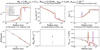 |
Fig. 10 Effect of local enhancements in the vertically integrated dust-to-gas mass ratio on the equilibrium solution by imposing fdg to be radially variable with a local Gaussian perturbation at various locations (see the dust-to-gas mass ratio profiles in Fig. F.3). The unperturbed value of fdg is the same for all the simulations, equal to 10−2. The ”5 au (10×)” case (blue) corresponds to dust enhancement at r = 5 au, where fdg varies from its unperturbed value to 10−1. The “5 au (5×)” case (dark orange) is similar to the previous case, but fdg goes up to 5 × 10⁻² instead. The “DZOE (10×)” case (green) corresponds to dust enhancement at the expected dead zone outer edge (DZOE) location for the fiducial model (r = 23 au), where fdg varies from its unperturbed value to 10−1. The “DZOE (5×)” case (red) is similar to the previous case, but fdg goes up to 5 × 10⁻² instead. The “60 au (10×)” case (purple) corresponds to dust enhancement at r = 60 au, where fdgvaries from its unperturbed value to 10−1. The “60 au (5×)” case (brown) is similar to the previous case, but fdg goes up to 5 × 10⁻² instead. The ”No dust enhancement” case (gray) corresponds to the fiducial model. The panels show the various steady-state profiles of some key quantities, for the model parameters M⋆ = 1 M⊙, L⋆ = 2 L⊙, Mdisk = 0.05 M⋆, adust = 1 μm, and αhydro = 10−4. Panels a–e show the same key quantities as in Fig. 7. Panel f: deviation from Keplerian velocity, where vϕ, gas is the azimuthal gas velocity and vK = rΩK is the Keplerian velocity. The dotted black line corresponds to vϕ, gas = vK. |
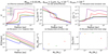 |
Fig. 11 Effect of stellar properties on the equilibrium solution when varying the parameters M⋆ and L⋆ together, all the way from accreting brown dwarfs to Herbig stars. The total disk gas mass does not depend on stellar mass and is such that Mdisk = 0.01 M⊙. The “star 1” case (blue) corresponds to a star of mass M⋆ = 0.05 M⊙ and bolometric luminosity L⋆ = 2 × 10⁻³ L⊙. The “star 2” case (dark orange) corresponds to a star of mass M⋆ = 0.1 M⊙ and bolometric luminosity L⋆ = 8 × 10⁻² L⊙. The “star 3” case (green) corresponds to a star of mass M⋆ = 0.3 M⊙ and bolometric luminosity L⋆ = 0.2 L⊙. The “star 4” case (red) corresponds to the fiducial model where the stellar mass is M⋆ = 1 M⊙ and the bolometric luminosity is L⋆ = 2 L⊙. The ”star 5” case (purple) corresponds to a star of mass M⋆ = 2 M⊙ and bolometric luminosity L⋆ = 20 L⊙. The panels show the various steady-state profiles of some key quantities, for the model parameters Mdisk = 0.05 M⋆, adust =1 μm, fdg = 10−2, and αhydro = 10−4. Panels a–f show the same key quantities as in Fig. 7. |
6.4 The effect of stellar properties
Finally, we explore how the stellar properties impact the equilibrium solution by running five simulations, covering the possible range from very low-mass to Herbig-like stars. For each star of interest, both the stellar mass and bolometric luminosity change and are taken from Table 3. Moreover, we avoided the effect of total disk gas mass on the equilibrium solution (see Sect. 6.1) by setting the total disk gas mass independent of stellar mass and equal to 0.01 M⊙. The results can be seen in Fig. 11.
Going from star 1 to star 5 model, both the stellar mass and bolometric luminosity increase (the latter way faster than the former). A higher bolometric luminosity leads to (slightly) higher gas temperature (see Eq. (4)), and higher stellar X-ray luminosity (LXR ∝ L⋆). Since the effect of gas temperature is weak and barely impacts on the MRI activity (see Appendix D.3), a higher bolometric luminosity implies a positive feedback on the MRI because it produces a higher stellar X-ray luminosity, generating more charged particles in the gas-phase.
Figures 11e and 11f show that star 4 and 5 models have a higher accretion rate and a more compact dead zone compared to star 1–3 models (the highest accretion rate and most compact dead zone are obtained for the star 5 model). One way to understand this result is by looking at Fig. 11c. We notice that the mid-plane ionization rate is much higher for star 4 and 5 models compared to star 1–3 models, with the distinctive shape seen in Sect. 6.1 for Mdisk = 0.005 M⋆ or Mdisk = 0.01, M⋆. Such a shape indicates that stellar X-rays utterly dominate the ionization process in most of the disk, included at the mid-plane. Since the ionization level is much higher for star 4 and 5 models, the nonideal effects are less stringent (see, e.g., Fig. 11d, where the optimal r.m.s. magnetic field strength is higher for star 4 and 5 models). As a result, the MRI can be moreeasily triggered (more compact dead zones) and the MRI-driven turbulence is stronger (higher accretion rates) for high-mass and more luminous stars.
Conversely, we notice a weaker dependence of RDZ and Ṁacc on M⋆ for star 1–3 models. With a subdominant ionization from stellar X-rays at the mid-plane, the significant increase in L⋆ (hence LXR) from star 1 to 3 model does not have as much impact as seen for star 4 and 5 models, since galactic cosmic rays dominate the ionization process at the mid-plane. As a result, RDZ and Ṁacc primarily depends on M⋆, and not on M⋆ and L⋆, as it is the case for star 4 and 5 models (RDZ depends on L⋆ only weakly through T for low-mass and less luminous stars). Since M⋆ weakly increases from star 1 to 3 model, we can explain the weaker dependence of RDZ and Ṁacc on M⋆ for low-mass and less luminous stars.
Finally, we note that the aspect ratio can be as large as 0.4 in the disk outer regions for star 1 and 2 models. We thus caution the reader that the profiles shown for these stars may not be valid for r ≳ 40 au, where the thin disk approximation reaches its limit (the aspect ratio is < 1, but not ≪ 1). Nevertheless, we do expect the global picture for the effect of stellar properties to still hold as described.
Here we investigated the effect of stellar properties alone by setting the total disk gas mass to the fixed stellar-independent value, Mdisk = 0.01 M⊙. However, this choice leads to very peculiar total disk gas masses relative to their stellar mass for the star 1 model (Mdisk = 0.2 M⋆) and the star 5 model (Mdisk = 0.005 M⋆). Although Mdisk = 0.2 M⋆ for the star 1 model, we note that the corresponding Toomre parameter Q is still higher than 2 at all radii, implying that the disk around this star is not self-gravitating. In Appendix D.4, we present a set of simulations with a stellar-dependent total disk gas mass (Mdisk = 0.05 M⋆), which represents a more realistic choice.
Summary of the viscous formation timescales for the potential steady-state pressure maxima formed by local dust enhancement at various locations in the protoplanetary disk.
Summary of the stellar parameters (mass, M⋆, and luminosity, L⋆) used to investigate the effect of stellar properties on the equilibrium solution.
7 Discussion
7.1 Gas structure
For steady-state accretion, we expect the mass flow through the disk to be uniform only if the disk is more massive at radii where the effective turbulent parameter  is lower (see Eq. (41)); namely, where the dead zone sits. For the fiducial model, we find that the dead zone indeed contains most of the gas content enclosed in the domain considered (67%). This has been previously seen by studies such as Terquem (2008). Here we confirm their result with a more consistent steady-state model that accounts for detailed considerations of the MRI with nonideal MHD effects (Ohmic resistivity and ambipolar diffusion), instead of a parametric version.
Terquem (2008) also shows that no steady-state pressure maximum at the dead zone outer edge is expected in a 1+1D approach (see their Fig. 3). We extend their study by showing that it holds only if dust accumulation has been inefficient at the dead zone outer edge before the disk reaches its steady-state accretion regime. The formation of a pressure bump at that location is indeed expected to be a transient phenomenon, since the gas pileup would be smeared out by density waves or Reynolds stress driven by the turbulent layers (see, e.g., Pinilla et al. 2016). However, if a sufficient amount of dust particles accumulate at the dead zone outer edge before the steady-state accretion regime is reached, the gas structure will display a steady-state pressure bump at that location, which can be formed within the disk lifetime (see Sect. 6.3.2), hence promoting further dust trapping.
A striking feature of our steady-state gas surface density profiles is the discontinuity at the dead zone outer edge (r = 23 au for the fiducial model). As mentioned in Sect. 5, this discontinuity arises from our on/off criteria for active MRI, inducing a steep change in the local turbulent parameter α at each transition from low to high turbulence regime. To confirm whether this is a real discontinuity in the mathematical sense or a numerical artifact due to a lack of resolution, we reran the fiducial model with a refined radial grid around the mid-plane dead zone outer edge (r = 23 au). With the much higher resolution that provides the refined radial grid (259 cells to describe the region ![Mathematical equation: $r \in \left[21, 25\right]\,$](/articles/aa/full_html/2022/02/aa41689-21/aa41689-21-eq155.png) au, instead of 9 cells for the fiducial radial grid), we still find that Σgas is discontinuous at that location. In reality, though, such a steep transition in the gas surface density would not happen: as proposed by Yang & Menou (2010), the gas would rearrange itself triggered by, for example, Rayleigh adjustment on a timescale shorter (close to the dynamical timescale) than the disk takes to reach its steady-state accretion regime (viscous evolution timescale). Consequently, we expect our steady-state accretion solution to be valid everywhere but at the transition between the dead zone and MRI-active layer, where the transition should be a smoother version of our solution. This discrepancy does not change the qualitative results drawn in this study.
au, instead of 9 cells for the fiducial radial grid), we still find that Σgas is discontinuous at that location. In reality, though, such a steep transition in the gas surface density would not happen: as proposed by Yang & Menou (2010), the gas would rearrange itself triggered by, for example, Rayleigh adjustment on a timescale shorter (close to the dynamical timescale) than the disk takes to reach its steady-state accretion regime (viscous evolution timescale). Consequently, we expect our steady-state accretion solution to be valid everywhere but at the transition between the dead zone and MRI-active layer, where the transition should be a smoother version of our solution. This discrepancy does not change the qualitative results drawn in this study.
As shown by Mohanty et al. (2018, see their Appendix B), the total inward accretion rate Ṁacc can always be decomposed, at each radius, as the sum of the accretion rates within the individual vertical layers of the disk (MRI-active layer, dead and zombie zone). Since we impose steady-state accretion, Ṁacc is radially constant in our equilibrium solutions. Doing so, though, means that the accretion rates within the individual layers are unavoidably radially variable, as there are no separate conditions to demand invariance. For example, we find for the fiducial model that the accretion rate within the dead zone is negative for r ≳ 10 au to compensate for the accretion within the MRI-active layer that exceeds the total value, hence ensuring that the total inward accretion rate, Ṁacc, is radially constant (see Fig. F.2). Consequently, we could expect the gas to build up at some locations or excavate at others (e.g., r = 10 au), hence driving the disk away from our equilibrium solution. To confirm that our solution is valid in a dynamical time-averaged sense, the local viscous evolution timescale – over which the buildup or excavation of gas changes the vertical density structure – must be much longer than the local dynamical timescale needed for the disk to relax back to a hydrostatic equilibrium vertical profile. In Fig. 12, we show the local viscous evolution timescale ( , where
  ) as well as the local dynamical timescale (
 ). Since we find tdyn ≪ tvisc everywhere, we can thus conclude that the gas volume density perturbations – induced by the variable accretion rates in the individual layers – are vertically smoothed out much more rapidly than they can grow and drive away the disk from our steady-state accretion solution. We confirm that it is the case for all equilibrium solutions presented in this work.
If the protoplanetary disk is at some stage of its evolution out of equilibrium, the gas surface density will change so that the disk evolves toward a steady-state (our solutions). The local viscous evolution timescale tvisc tells us in how much time the steady-state accretion is reached, at a given radius, assuming that the disk is purely viscously evolving. For the fiducial model, we find that tvisc is in the range 0.4 − 2.7 Myrs; with a mean value of 1.5 Myr in the dead zone and 1 Myr in the MRI-active layer (see Fig. 12, where the longest viscous evolution timescale is reached in the dead zone at r ≈ 15 au). The steady-state accretion regime can thus be established, at most radii, within the disk lifetime, particularly before the disk dispersal phase by, for example, internal photoevaporation that can disperse the gas content after 1 − 4 Myrs of evolution (see, e.g., Owen & Kollmeier 2019; Kunitomo et al. 2021). Consequently, the protoplanetary disk could accumulate a spatially extended long-lived inner disk gas reservoir (the dead zone) accreting a few times 10−9 M⊙ yr−1, before photoevaporation starts carving a hole; possibly resulting in transition disks with large gaps and high accretion rates once photoevaporation starts being at play (see Gárate et al. 2021).
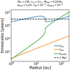 |
Fig. 12 Various local timescales, as a function of radius, for the fiducial model described in Sect. 5. The solid blue line (tvisc) corresponds to the viscous evolution timescale. The solid orange line (tdyn) corresponds to the dynamical timescale. The solid green line (tgrowth) corresponds to the growth timescale for the case of micron-sized particles. The dashed black line corresponds to 1 Myr. |
7.2 Accretion rates for different stellar masses
In steady-state accretion models such as ours, there is a tight correlation between the total disk gas mass and the accretion rate (see Fig. 7e). In principle, for given stellar and dust properties, we could estimate the total disk gas mass from an observed accretion rate (assuming that the disk has reached a steady-state MRI-driven accretion regime).
We performed this exercise with the results reported in Manara et al. (2017). In their work, the authors present a study of a sample of 94 young stars with disks in the Chamaeleon I star-forming regions (1 − 6 Myr; see van der Marel & Mulders 2021, their Table 1 and references therein). They analyze the spectra of those objects obtained with the ESO VLT/X-shooter to derive, among others, the Ṁacc − M⋆ relation. Manara et al. (2017) show that this relation could be better described with a model more complex than a “single-line” fit (although the single-line fit is not statistically excluded): a “segmented-line” fit with a break at M⋆ ≈ 0.3 M⊙, delimiting a linear relation at higher M⋆ and steeper relation at lower M⋆. We present the single-line as well as the segmented-line best-fit models in Fig. 13, with the 1σ dispersion around the former (gray area). From our ends, we ran six simulations corresponding to a total disk gas mass Mdisk ∈{0.001, 0.002, 0.005, 0.01, 0.05, 0.10} M⋆, for each stars taken from Table 3. The results are shown in Fig. 13.
To quantitatively match the accretion rates of very low-mass and less luminous stars (star 1 and 2 models) obtained from the Manara et al. (2017) Ṁacc − M⋆ relation, we find that their total disk gas mass must be lower compared to the more massive and luminous counterparts (star 3–5 models). For star 1 and 2 models, Fig. 13 shows that the two best-fit models from Manara et al. (2017) are consistent with a total disk gas mass that is roughly in the range 0.002 M⋆–0.005 M⋆. Conversely, for star 3 and 4 models, the two best-fit models are consistent with a total disk gas mass that is roughly in the range 0.01 M⋆–0.05 M⋆, whereas they are consistent with a total disk gas mass that is roughly in the range 0.01 M⋆–0.10 M⋆ for the star 5 model. Our results support the ideas that the steeper relation seen in the accretion rates for very low-mass and less luminous stars may be caused by: (1) a faster evolution, since we need a total disk gas mass values that are nowadays low; or (2) the fact that very low-mass and less luminous stars initially form with a low total disk gas mass (relative to their stellar mass). Previous studies suggest that the faster evolution of disk around very low-mass stars could be explained by faster accretion, since these disks could potentially be entirely MRI active (e.g., Hartmann et al. 2016). However, as seen in Sect. 6.4 (also see, Mohanty et al. 2013a), this idea seems unlikely because ambipolar diffusion becomes stronger at the low densities expected for the disk around those stars, hence preventing the MRI from easily operating everywhere. Without any other mechanisms to explain faster evolution in the context of MRI-driven accretion, the idea of very low-mass and less luminous stars being initially formed with a lower total disk gas mass compared to high-mass and more luminous stars seems more probable.
We note that our accretion rates presented in Fig. 13 depend on the choice made for rmax, the outer boundary of our radialgrid (rmax = 200 au in this study). For fixed model parameters and given a field strength, the steady-state accretion solution is unique. By solely varying rmax, we change how the gas mass is distributed in space: a lower rmax implies higher gas surface densities (since the same amount of gas is now distributed across a more confined domain), whereas a higher rmax leads to lower ones. We find that both the accretion rate and the dead zone maximal radial extent increase with decreasing rmax (not shown here). The former dependence can be explained by the fact that a lower rmax means less distance for the gas to travel before being accreted onto the central star. The latter dependence is justified by the fact that a lower rmax implies an overall lower ionization level in the disk. Consequently, all the accretion rates presented in Fig. 13 are expected to increase if rmax < 200 au, and decrease if rmax > 200 au. Additionally, we find that the effect of rmax is more prominent for lower total disk gas masses (not shown here). Nonetheless, the main conclusions of this section do not change. Indeed, the gas radius for a disk around a very low-mass and less luminous star is more likely to be lower than our fiducial 200 au (see, e.g., Kurtovic et al. 2021), and also lower than the gas radius for a disk around a high-mass and more luminous star. As a result, the accretion rate of a very low-mass and less luminous stars is expected to increase compared to what is displayed in Fig. 13, implying that even lower total disk gas masses will be needed to explain the steeper relation seen in the accretion rates.
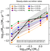 |
Fig. 13 Accretion rate as a function of stellar mass. The dash-dotted and solid black lines correspond to the single-line and segmented-line best-fit models, respectively, from Manara et al. (2017). The 1σ dispersion around the single-line best-fit model is shown by the gray area. The “+” symbols represent the accretion rates obtained for various total disk gas masses and for each star taken from Table 3, using our steady-state accretion model. Here we assume that adust =1 μm, fdg = 10−2, and αhydro = 10−4. |
7.3 The need for gas, dust, and stellar evolution
The detailed parameter study conducted in Sect. 6 shows that the following parameters play a crucial role in shaping the steady-state accretion solution: (1) the total disk gas mass; (2) the representative grain size; (3) the vertically averaged dust-to-gas mass ratio; and (4) the stellar X-ray luminosity. In general, those parameters may change during the evolution of the protoplanetary disk. We will thus need to relax the steady-state accretion assumption in future studies. Doing so means that we will need to implement some missing ingredients.
First, we will need to consider gas evolution. During the evolution of class II protoplanetary disks, the gas content is removed from the disk due to accretion onto the star and winds (e.g., magnetocentrifugal or photoevaporative). Additionally, there is no source term as in class 0/I disks, where the envelope in-fall can feed in gas. In general, the total disk gas mass thus inevitably decreases over time. In Sect. 6.1, we saw that the equilibrium solution strongly depends on the total disk gas mass with which the disk reaches its steady-state accretion regime: a lower total disk gas mass implies a lower accretion rate, and a more compact dead zone. Consequently, for a given initial total disk gas mass, we expect the gas surface density to start evolving toward the equilibrium solution corresponding to this total disk gas mass. Since the total disk gas mass decreases over time, the gas surface density will readjust by evolving toward a new steady-state solution corresponding to that new total disk gas mass. Gas evolution is crucial here since it will tell us how the gas structure changes over time and, hence, from what steady-state solution to another the disk will tend, assuming pure viscous evolution.
Second, we will need to implement dust evolution, including growth processes. Here we assumed a fiducial vertically averaged dust-to-gas mass ratio of 10−2 and small dust grains of constant size 1 μm. Such values may be expected in the early stages of dust evolution in the disk. However, dust particles grow, fragment, drift, stir and settle during the evolution of protoplanetary disks. In the case of our fiducial model, Fig. 12 shows that micron-sized grains grow on a timescale (tgrowth) that is shorter than the timescale the gas needs to evolve on large scales (viscous evolution timescale tvisc), for r ≲ 60 au. Here tgrowth is computed using the mid-plane value of Eq. (30) from Birnstiel et al. (2016), where we take the relative velocity Δv to be the Brownian relative velocity defined as  , with mred the reduced mass (mred = mdust∕2 for a collision of equal micron-sized grains. On one hand, it implies that our steady-state accretion solution may describe well the gas for r ≳ 60 au because such a regime can be reached before micron-sized grains can grow substantially. On the other hand, dust growth becomes important for r ≲ 60 au. In Sects. 6.2 and 6.3, we found that both a larger grain size and a higher dust depletion imply a higher accretion rate, a higher
  overall, and a more compact dead zone. Consequently, we would expect the following cycle to happen, where the disk turbulence state oscillates between a low and high regime. For the initial conditions Mdisk = 0.05 M⋆, adust = 1 μm and fdg = 10−2, the gas will start evolving toward the corresponding equilibrium solution. Since tgrowth ≤ tvisc for r ≲ 60 au, the dust can efficiently grow by coagulation to representative grain sizes skewed toward larger sizes in such regions, and the vertically averaged dust-to-gas mass ratio of micron-sized grains can substantially drop before this steady-state accretion solution can actually be reached. As a result, the gas will evolve toward a new equilibrium solution corresponding to a disk with a higher
  overall. A higher
  in the disk implies a more efficient fragmentation that can replenish micron-sized grains. The representative grain sizes can thus be skewed toward micron-sized particles again, and the vertically averaged dust-to-gas mass ratio of micron-sized grains can re-increase, resulting in the gas evolving toward a steady-state solution close to the initial one, corresponding to a less turbulent disk. Due to a low disk turbulence level, the dust can effectively grow and less frequently fragment again, hence looping the cycle. A similar cycle has been reported in Okuzumi & Hirose (2012) where growth, settling and fragmentation were considered alongside Ohmic resistivity (see their Fig. 3). The authors find that this cycle is actually a ”damped oscillation,” that is to say, the disk turbulence state and grain size distribution converge and stop oscillating rather than indefinitely oscillating. The equilibrium solution corresponding to Mdisk = 0.05 M⋆, adust = 1 μm, and fdg = 10−2 is thus physically motivated if the cycle mentioned above can be completed on a timescale shorter than the viscous evolution timescale (otherwise the total disk gas mass decreases) and the drift timescale (otherwise dust particles are removed from the disk, and the overall dust content drops), and if the grain size distribution at the end of the cycle is comparable to the one at the beginning of the cycle (i.e., the grain size distribution is skewed toward micron-sized grains). Additionally, we note that such a cycle is also likely to happen in the steady-state pressure maxima generated by local dust enhancements (see Sect. 6.3.2), possibly generating pressure maxima that could “come and go” over time. In order to provide amore consistent picture for this cycle, we need a time-dependent framework with dust evolution included.
Finally, stellar evolution will need to be accounted for. As we saw in Sect. 6.4, the stellar X-ray luminosity LXR plays a fundamental role because it quantifies how much the gas can be ionized by stellar X-rays: the higher the stellar X-ray luminosity is, the more turbulent the disk is overall. Depending on the stellar type, this quantity is more or less constant over time (see, e.g., Kunitomo et al. 2021, their Fig. 5). As a result, a time-dependent framework needs to consider the time-dependence of LXR.
7.4 Model limitations and justification for model assumptions
In our 1+1D global MRI-driven disk accretion model, we adopt seven simplifications. First, we focus our study on the MRI-driven accretion and assume maximal efficiency for the MRI activity. For this assumption to hold, the disk must be threaded by a net vertical magnetic field; otherwise, the MRI is very inefficient (Simon et al. 2013b). In the presence of a net vertical field, though, it seems inevitable for the disk to launch a magnetized wind that efficiently carries angular momentum away and drives accretion at rates consistent with observations (see, e.g., Blandford & Payne 1982; Bai & Stone 2013; Lesur 2021). To be consistent with the assumption of maximal efficiency for the MRI activity, wind-driven accretion thus needs to be included in our model in the future. Furthermore, the highest accretion rate reached by our various steady-stateMRI-driven accretion models for a disk around a solar-type star corresponds to the canonical value Ṁacc ≈ 10−8 M⊙ yr−1 (for Mdisk = 0.13 M⋆, adust = 10 μm, fdg = 10−3, and αhydro = 10−4). Nonetheless, it seems that this value can only be reached for a disk close to be self-gravitating. For typical class II disks, MRI/wind hybrid models are thus necessary to capture the turbulence level in the disk (wind and MRI-driven accretion can coexist as shown by Cui & Bai 2021).
Second, we assume that the MRI activity is at the maximal efficiency as permitted by Ohmic resistivity and ambipolar diffusion. Such a condition is fulfilled by constraining and adopting the magnetic field strength so that it corresponds to the highest field strength that would still allow the MRI to operate. In reality, there are no clear reasons why the field would follow such a configuration. Actually, there is ample evidence from MHD simulations that the saturation level of the MRI-driven accretion stress is controlled by the strength of the net vertical magnetic field, (e.g., Hawley et al. 1995; Suzuki et al. 2010; Okuzumi & Hirose 2011; Simon et al. 2013a,b). In principle, the radial distribution of the net vertical magnetic flux is determined by the diffusion and advection of the large-scale field lines, although its details are yet to be fully understood (e.g., Lubow et al. 1994; Guilet & Ogilvie 2014; Okuzumi et al. 2014; Takeuchi & Okuzumi 2014; Bai & Stone 2017; Zhu & Stone 2018). As such, a more consistent picture could be obtained by combining our calculations of the nonideal MHD terms (magnetic diffusivities) – derived from a careful modeling of the gas ionization degree – to 3D MHD simulations where the magnetic field strength would be solved self-consistently (beyond the scope of this paper).
Third, we consider stellar X-rays, galactic cosmic rays, and the decay of short- and long-lived radionuclides as the main ionization sources. In this approach, two important ionization sources are neglected: far-ultraviolet (FUV) and stellar energetic particles (SPs). (1) FUV can fully ionize atomic carbon and sulfur. Perez-Becker & Chiang (2011) show that FUV can penetrate a vertical gas column density ΣFUV ∈ [0.01 − 0.1] g.cm−2, and produce much higher ionization than other sources. Additionally, Simon et al. (2013a) found that the MRI is the most effective in the FUV layer in the outer disk. Depending at which disk height the penetration depth ΣFUV is reached, FUV could thus be important and needs to be included in future works. (2) Stellar energetic particles become the dominant H2 ionization source in the warm molecular layer of the disk above the CO ice line, and can increase the column densities of HCO+ by a factor in the range 3−10 for disk radii r ≲ 200 au, with a higher impact in the disk regions with low cosmic ray ionization (see Rab et al. 2017). The inclusion of the SPs could change our equilibrium solution because it could boost the ionization level and thus impact the number density of HCO+. This effect should be included in future studies.
Fourth, for the disk dust structure, grains are assumed to be a mono-disperse population of size adust. In reality, protoplanetary disks have a distribution of grain sizes determined by the balance between collisional coagulation, fragmentation and radial drift. One of the main goals for a future work is to self-consistently implement a size distribution directly from dust evolution models. For simplicity, we also do not consider the sublimation of water ice, and thus the change in dust properties across the protoplanetary disk. Furthermore, we assume that the vertical dust density follows a Gaussian distribution (e.g., Pinte et al. 2008, when attempting to interpret dust continuum observations). Nevertheless, this assumption may not hold at high altitude in the protoplanetary disk, as seen in studies of dust settling driven by the MRI in the ideal MHD limit (see Fromang & Nelson 2009).
Fifth, for the disk gas structure, we assume the gas to be vertically isothermal, and passively heated by stellar irradiation. Here we neglect viscous heating. This could be added in future studies by solving for the self-consistent disk vertical structure adopting a similar approach described in, for example, D’Alessio et al. (1998, 1999), and Jankovic et al. (2021). Nevertheless, we do not expect such an implementation to change our results because viscous heating is inefficient in the dead zone (Hirose & Turner 2011; Mori et al. 2019, 2021) as well as in the regions where the MRI can operate (low gas density).
Sixth, in addition to the magnetic disk winds, we also neglect some processes that could drive the angular momentum transport: (1) the Hall shear instability (HSI) causing strong radial angular momentum transport if the magnetic field is aligned with the rotation axis of the protoplanetary disk (see, e.g., Kunz 2008; Lesur et al. 2014; Bai 2015); (2) gravito-turbulence that may arise in regions of the disk where the enclosed local disk gas mass is such that Q ≈ 2, with a cooling timescale longer than the orbital timescale (see, e.g., Béthune et al. 2021). For the latter, the total disk gas mass of all our disk models has been chosen such that the Toomre parameter Q is always higher than 2 (≈ 3 in practice). The gravito-turbulence is thus expected not to dominate the disk turbulence state in our steady-state accretion solutions.
Seventh, we assume that HCO+ is the only ion species in the gas-phase, reflecting the fact that CO is the most abundant molecule after H2. However, this assumption may not hold everywhere in the disk. For temperatures below 25 K (CO freeze-out), the dominant ions are  , where x = 1, 2, 3. In the disk inner part where T ≳ 100 K, the metal ion Mg+ can desorb from the solid grains and tend to recombine in longer timescales (Dzyurkevich et al. 2013). Nonetheless, we do not expect such ions to significantly modify our equilibrium solutions for 25 K ≲ T ≲ 100 K.
8 Summary and conclusions
We present a 1+1D global framework to study the outer protoplanetary disk (r ≳ 1 au), which accretes viscously solely due to the MRI and hydrodynamic instabilities. The disk is heated by stellar irradiation and ionized by stellar X-rays, galactic cosmic rays, and radionuclides. A semi-analytical chemical model is employed to capture the charge state of the disk dust-gas mixture, hence carefully modeling the gas ionization degree. Additionally, the magnetic field strength is constrained and adopted for the MRI activity to be at the maximal efficiency as permitted by our set of conditions for active MRI. For given stellar and disk parameters, the effective viscosity parameter,  , can thus be determined self-consistently under the framework of viscously driven accretion from detailed considerations of the MRI with Ohmic resistivity and ambipolar diffusion.
We employ our framework to investigate the structure of a steadily accreting protoplanetary disk. To obtain the steady-state MRI-driven accretion solution corresponding to the MRI activity at maximal efficiency, the gas surface density, gas ionization state, magnetic field, viscosity, and accretion rate are calculated self-consistently.
For the fiducial protoplanetary disk model considered, we find that:
The accretion rate reached by this disk model is Ṁacc ≈ 3.7 × 10⁻⁹ M⊙ yr−1, the mean effective turbulence level in the MRI-active layer is
 , and the dead zone maximal radial extent is RDZ = 23 au. For studies using an ad hoc prescription for the Shakura–Sunyaev viscosity parameter α, a value of a few times 10−3 is found to be more appropriate for describing the viscosity in the MRI-active layer, accounting for ambipolar diffusion;
The steady-state accretion regime of such a disk is reached within the disk lifetime, particularly before the disk dispersalphase. The disk could thus accumulate a spatially extended long-lived inner disk gas reservoir before internal photoevaporation starts carving a hole;
A steady-state pressure maximum does not form at the dead zone outer edge;
Ambipolar diffusion quenches the MRI activity over most of the disk. The upper envelope of the MRI-active layer is set by ambipolar diffusion, whereas Ohmic resistivity primarily sets its lower envelope.
Additionally, we perform an exhaustive parameter study to investigate what model parameters are crucial to the MRI-driven accretion in protoplanetary disks, as well as the extent to which the accretion is efficient (namely, the location of the dead zone outer edge and the value of the accretion rate). We adopt the fiducial parameters but vary the following model parameters one at a time: the total disk gas mass (Mdisk), the representative grain size (adust), the vertically averaged dust-to-gas mass ratio (fdg), the stellar properties (both M⋆ and L⋆), the hydrodynamic turbulent parameter (αhydro), and the gas temperature model (T). We find that:
The accretion rate and dead zone outer edge location as a function of the total disk gas mass are approximately power laws:
 and
and  . A more massive disk implies a higher accretion rate and a more extended dead zone (both radially and vertically);
A smaller grain size leads to a smaller accretion rate and a more extended dead zone. When submicron dust particles are considered (adust = 0.1 μm), the disk mid-plane is mainly MRI-dead and accretes much more slowly. Furthermore, the steady-state solution remains unchanged regardless of the grain size for adust ≳ 100 μm. This suggests that there exists a threshold for the grain size above which the grains have little impact on the ionization chemistry, and hence little impact on the MRI;
An overall higher depletion of micron-sized grains leads to a higher accretion rate and a more compact dead zone. Dust enhancement (fdg = 10−1) compared to the standard ISM value strongly damps the MRI-driven accretion. Additionally, the steady-state accretion solution is independent of the vertically integrated dust-to-gas mass ratio choice for fdg ≲ 10−4. As a result, there exists a threshold for the depletion of micron-sized grains below which the grains have little impact on the ionization chemistry, and hence little impact on the MRI;
If a sufficient amount of dust particles has locally accumulated in a region where the MRI can operate before the disk reaches its steady-state accretion regime, the gas structure will adjust to form a steady-state pressure maximum close to the location of dust enhancement. These spontaneous steady-state pressure maxima can be formed within the disk lifetime, which might have direct consequences for planet formation by promoting further dust trapping;
For a fixed stellar-independent total disk gas mass, a more massive and luminous star implies a higher accretion rate and a more compact dead zone;
The accretion rate and dead zone outer edge location as a function of the hydrodynamic turbulent parameter are approximately power laws:
 and
and  . A higher αhydro leads to a higher accretion rate and a more extended dead zone. For αhydro = 10−3, the gas surface density profile is much smoother (Σgas ∝ r−1.22) than the profiles obtained for lower αhydro values and is actually close to the constant-α model solution (Σgas ∝ r−1);
The choice for either an optically thin or thick radial gas temperature model has little impact on the accretion rate, dead zone size, or the overall equilibrium solution.
Finally, we investigate in more depth the effect of stellar properties by considering more realistic models in which the total disk gas mass is stellar-dependent. We find that:
For a fixed stellar-dependent total disk gas mass, a more massive and luminous star implies a higher accretion rate and a more extended dead zone;
The dead zone cannot become indefinitely large for high-mass and more luminous stars, since their high stellar X-ray luminosity regulates its radial extent. Similarly, the dead zone cannot become indefinitely small for low-mass and less luminous stars due to their too low stellar X-ray luminosity;
For the range of stars considered (0.05 M⊙− 2 M⊙), ambipolar diffusion is the primary factor determining the strength of the MRI-driven accretion;
To explain the steeper relation seen in the observed accretion rates of very low-mass and less luminous stars (Manara et al. 2017) in the context of MRI-driven accretion, we find that very low-mass and less luminous stars need to be initially formed with a lower total disk gas mass compared to the high-mass and more luminous counterparts.
In summary, we show that the MRI-driven accretion behavior crucially depends on the total disk gas mass, the representative grain size, the vertically integrated dust to gas ratio, and the stellar X-ray luminosity. Since those quantities are expected to undergo substantial change throughout the evolution of the disk, we need to relax the steady-state assumption and account for gas, dust, and stellar evolution. Furthermore, we show that dust accumulation at specific locations in the disk can lead to the spontaneousformation of steady-state pressure maxima. This strongly motivates the combination of dust evolution with careful modeling of the gas ionization degree in a time-dependent framework. Consequently, a self-consistent time-dependent coupling between gas, dust, stellar evolution models, and our framework on million-year timescales is required in future studies.
Acknowledgements
We are thankful to the anonymous referee for the very detailed and constructive report. We thank Christelle Delage and Reema Joshi for providing great comments on the manuscript. We thank Marija Jankovic, Giovanni Rosotti, Dmitry Semenov, Carlo Manara and Nicolás T. Kurtovic for fruitful discussions and very useful insights. This work made extensive use of the Astropy (Astropy Collaboration 2013), Matplotlib (Hunter 2007), Numpy (Harris et al. 2020), Scipy (Virtanen et al. 2020) software packages. T.N.D. and P.P. acknowledge support provided by the Alexander von Humboldt Foundation in the framework of the Sofja Kovalevskaja Award endowed by the Federal Ministry of Education and Research. S.O. is supported by JSPS KAKENHI Grant Numbers JP18H05438, JP19K03926, JP20H01948, and 20H00182. M.F. acknowledges funding from the European Research Council (ERC) under the European Union’s Horizon 2020 research and innovation program (grant agreement no. 757957). N.D. acknowledges support provided by DFG under grant DU 414/20-1 (SPP 1992).
Appendix A Derivation of Eqs. (20)–(24)
In this section we derive the equations that describe the gas–dust charge reaction equilibrium, Eqs. (20)–(24). We basically follow the derivation by Okuzumi (2009), but take the induced polarization force between ions/free electrons with charged grains into account. We begin with the equations describing the time evolution of ni and ne due to ionization and recombination,
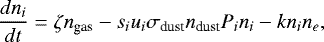 (A.1)
(A.1)
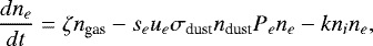 (A.2)
(A.2)
where Pi(e) is the effective cross section averaged over grain charge Z and normalized by si(e)σdust,
 (A.3)
(A.3)
with  is the normalized effective cross sections for grains of charge Z and the brackets denote an average over Z. Accounting for the induced polarization forces and assuming Z < 0 (see the main text), we use Eqs. (3.3) and (3.5) of Draine & Sutin (1987):
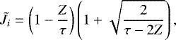 (A.4)
(A.4)
 (A.5)
(A.5)
In comparison, Okuzumi (2009) adopted  and
and  for Z < 0 by neglecting the polarization forces.
In ionization–recombination equilibrium with dni∕dt = 0 and dne∕dt = 0, Eqs. (A.1) and (A.2) reduce to two algebraic equations for ni and ne. These equations can be easily solved to yield Eqs. (23) and (24) (see Okuzumi 2009, for a similar calculation).
To derive the equilibrium grain charge distribution, we follow the Appendix of Okuzumi (2009) and write down the detailed balance equation,
 (A.6)
(A.6)
For τ≳1, the grain charge distribution satisfies  and hence can be viewed as a continuous function of Z (see the Appendix of Okuzumi 2009). In this case, one has
  and ndust(Z + 1) ≈ ndust(Z) + dndust∕dZ, and therefore Eq. (A.6) approximately reduces to
 (A.7)
(A.7)
where
 (A.8)
(A.8)
To derive an approximate solution for (A.7), we define Z0 such that W(Z0) = 0 (i.e.,  ) and δZ≡ Z − Z0. To the first order in δZ, one has
 (A.9)
(A.9)
With Eq. (A.9), Eq. (A.7) can be analytically solved, yielding ndust(Z) given by Eq. (20) with ⟨Z⟩ = Z0 and
 (A.10)
Finally, by approximating  and using ⟨Z⟩ = −Γτ, we obtain Eq. (22). A complete expression of Eq. (22) is
![Mathematical equation: \begin{eqnarray*}\langle\Delta Z^2 \rangle&=&{\tau} \left[\frac{2 \Gamma \tau +3 \sqrt{\Gamma \tau}}{2\left(\sqrt{\Gamma \tau}+1\right){}^2}+\frac{1}{\Gamma +1}\right.\nonumber \\&& \quad -\frac{\sqrt{2}}{(2 \Gamma +1) \left((2 \Gamma +1) \sqrt{\frac{\tau}{2 \Gamma +1}}+\sqrt{2}\right)}\nonumber \\&& \left. \quad +\frac{3}{(3 \Gamma +4){}^2 \sqrt{\frac{1}{3 \Gamma +4}}\left(\sqrt{\frac{1}{3 \Gamma +4}}+\sqrt{\tau}\right)}\right]^{-1}.\end{eqnarray*}](/articles/aa/full_html/2022/02/aa41689-21/aa41689-21-eq187.png) (A.11)
(A.11)
Appendix B Comparison between the semi-analytical chemical model and a chemical reaction network
We aim to validate the semi-analytical chemical approach used in this study (adapted from Okuzumi 2009) by comparing with a chemical reaction network. Particularly, we use the chemical reaction network by Umebayashi & Nakano (1980). We include the following charged species: free electrons, five ion species (H+, H , HCO+, He+, and C+) and charged grains. Among these, HCO+ represents heavy molecular ions (e.g., H3 O+) that recombine with free electrons dissociatively, and therefore at similar recombination rates. We neglect metal ions, assuming that all metal elements are locked into grains. The grains are allowed for a discrete charge distribution Z ∈ [Zmin, Zmax] with
  and
and  , where ⟨Z⟩ and
  are the mean grain charge and grain charge dispersion predicted from the semi-analytical model given by Eqs. (21) and (22), respectively. The radial and vertical profiles for the temperature, gas and dust densities as well as the total ionization rate are taken from the equilibrium solution obtained for the fiducial model described in Sect. 5.
We calculate the abundances of various charged species in local ionization–recombination equilibrium for 0 ≤ z∕Hgas ≤ 5, at r = 5 au and r = 100 au. Figure B.1 shows the results of the chemical network calculations. We plot the vertical profiles of the free electron abundance, total ion abundance, and the abundances of individual ion species. The results show that the dissociatively recombining molecular ions HCO+ are the dominant ions at all locations in the disk, except in the upper layers (z ≳ 4 Hgas) of the disk outer regions. In such high-altitude regions, though, the gas density is so low that it does not significantly impact our equilibrium solution (the solution is determined by  , which is a pressure-weighted vertically averaged quantity). Consequently, the assumption that HCO+ is the dominant ion species in most of the protoplanetary disk – made for the semi-analytical model employed in this study – is a good approximation. Figure B.1 also displays the free electron and total ion abundances from the semi-analytical model. At r = 5 au (resp., r = 100 au), we find the semi-analytical calculations to be in good agreement with the chemical network for all z ≲ 5 Hgas (resp., z ≲ 4 Hgas). At r = 100 au and for z ≈ 4 Hgas, the semi-analytical calculations slightly underestimate the free electron and total ion abundances, since the slowly recombining ion species H
 and C+ become as important as the fast recombining HCO+. However, the relative error between the chemical network and semi-analytical results is no larger than 40%. This discrepancy becomes larger for 4 < z∕Hgas ≲ 5 because HCO+ are no longer the dominant ions species. In these regions, the semi-analytical calculations can underestimate the free electron and total ion abundances up to a factor of ≈ 5 (at z = 5 Hgas). Nevertheless, the gas density is very low there, which means that our equilibrium solution is not sensitive to this discrepancy.
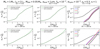 |
Fig. B.1 Comparison between the semi-analytical chemical model employed in this study and a chemical reaction network, for the fiducial model described in Sect. 5. The panels show various species abundances as a function of height, z, at r =5 au and r = 100 au (upper and lower rows, respectively). Left panels: Free electron abundance from the chemical reaction network (solid green lines) and the semi-analytical model (dotted black lines). Central panels: Total ion abundance from the chemical reaction network (solid green lines) and the semi-analytical model (dotted black lines). Right panels: Abundances of individual ion species from the chemical reaction network. The solid black line corresponds to HCO+, the solid blue line to H |

Appendix C The stellar X-ray ionization rate
To compute the stellar X-ray ionization rate (Eq. (11)), we used the fit from Bai & Goodman (2009), which is expressed as a function of vertical gas column densities. The underlying assumption is that the stellar X-rays penetrate the gas in the vertical direction, at any distance from the star. Although this approximation is good enough for galactic cosmic rays that originate from outside the protoplanetary disk, stellar X-rays are launched from around the central star. Depending on the exact location from where they originate (e.g., stellar surface or stellar jets), the use of vertical gas column densities to calculate the stellar X-ray ionization rate might become invalid.
For example, Fig. C.1 shows that stellar X-rays can efficiently penetrate and ionize the outer regions of the disk (via the direct X-ray contribution). In reality, this may not be the case if they have to penetrate the dense inner regions before reaching the outer ones: This extinction phenomenon corresponds to the self-shadowing event. It is expected to arise if stellar X-rays are launched from low-altitude regions, such as the stellar surface. In this case, the direct contribution is quickly extinguished due to its small penetration depth, and the scattered contributionis substantially modified since scattered stellar X-rays originate from direct stellar X-rays. Conversely, if stellar X-rays are launched from high-altitude regions above the disk mid-plane, such as the stellar jets, they can travel without having to penetrate the dense inner regions and thus reach and ionize the outer regions of the disk.
To properly account for the self-shadowing event, one solution could be to implement ray tracing in our framework. However, doing so would greatly increase the computational complexity of the whole problem. Given our main goal (combining detailed considerations of the MRI with nonideal MHD effects to gas and dust evolution models), we assumed in this study that the stellar X-rays originate from high-altitude regions around the central star (e.g., stellar jets), so that the stellar X-ray ionization rate’s fit given by Bai & Goodman (2009) holds.
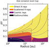 |
Fig. C.1 Ionization rate for H2 ζ(H2) (defined in Sect. 2.3) and its different contributions, as a function of location in the disk, for the fiducial model described in Sect. 5. For each color, the following nonthermal ionization source dominates ζ(H2): decay from short- and long-lived radionuclides (black), galactic cosmic rays (purple), or stellar X-rays (orange and yellow for the scattered and direct contribution, respectively). The solid colored contour lines correspond to the surfaces of constant total ionization rate, ζ(H2), ranging from7.6 × 10−19 s−1 to 1.8 × 10⁻¹⁰ s−1. The dashed white lines correspond to the surfaces z = 1 Hgas, z = 2 Hgas, z = 3 Hgas, and z = 4 Hgas, from bottom to top, respectively. |
Appendix D Follow-up parameter study
In this appendix we extend the parameter study conducted in Sect. 6 by performing a series of simulations that investigate: (1) the effect of magnetic field strength (Appendix D.1); (2) the effect of hydrodynamic turbulent parameter αhydro (Appendix D.2); (3) the effect of gas temperature model T(r) (Appendix D.3); (4) the combined effect of stellar properties and total disk gas mass (Appendix D.4). We deriveand show the same key quantities reached by our steady-state accretion disk model as in Sect. 6.
D.1 The effect of magnetic field strength
In this present work, all the derived accretion rates Ṁacc represent the highest value possibly reachable given the set of criteria for active MRI employed. Indeed, we adopt the magnetic field strength required for the MRI activity to be at maximal efficiency (see Sect. 3.2). Here we explore – for the fiducial parameters (M⋆ = 1 M⊙, L⋆ = 2 L⊙, Mdisk = 0.05 M⋆, adust = 1 μm, fdg = 10−2 and αhydro = 10−4) – what would be the derived accretion rates for either weaker or stronger magnetic field strengths, and show that our choice for the magnetic field strength leads to the highest value for the accretion rate as expected.
To do so, we assumed various constant mid-plane β-plasma parameters βmid such that βmid ∈{10, 102, 103, 104, 105}, calculated the corresponding r.m.s. mid-plane magnetic field strength  , and assumed that B is vertically constant. The results can be seen in Fig. D.1.
For βmid = 10, ambipolar diffusion utterly prohibits any MRI-driven turbulence at any locations in the disk because the magnetic field strength is too strong; leading to  at every radii, hence to the lowest accretion rate. For βmid = 102, the MRI can only operate in regions beyond 54 au (there is no MRI-active layer sitting above the dead zone for r ≲ 54 au). Although the effective turbulence is higher in such regions for this scenario compared to the optimal one, the mid-plane dead zone outer edge is roughly located as twice as far, implying that the accretion rate is overall lower. For βmid = 103, the field strength is such that the MRI can only operate in the upper layers for r ≳ 10 au, and from the mid-plane for r ≳ 30 au. Since this field strength is overall lower than the one constrained for the optimal scenario in the MRI-active layer, the local MRI-driven turbulence is weaker (hence lower
  ). Finally, for βmid = 104 and βmid = 105, the MRI can only effectively operate in the surface layers (there is no longer a mid-plane MRI-active layer). On one hand, for βmid = 104, we find that the MRI could in theory develop at the mid-plane for r ≳ 100 au. In practice, though, the induced mid-plane αMRI = 3.3 × 10⁻⁵ (radially constant) is less than αhydro = 10−4. As a result, we consider such regions as dead by fiat (see Eq. (39)). On the other hand, for βmid = 105, we find that the MRI cannot operate at the mid-plane because Eq. (30) is not fulfilled. Consequently, the mid-plane is weakly turbulent for both cases (
 ), since the MRI-active layer is located too high in the disk atmosphere to significantly contribute to the effective turbulence level.
D.2 The effect of the hydrodynamic turbulent parameter
Previous work on hydrodynamic instabilities suggest that αhydro could approximately range from 10−5 to 10−3 (see, e.g., Urpin & Brandenburg 1998; Klahr & Bodenheimer 2003; Nelson et al. 2013; Raettig et al. 2013; Lin & Youdin 2015; Manger et al. 2020; Flock et al. 2020; Barraza-Alfaro et al. 2021). In our study, we chose the fiducial value αhydro = 10−4 motivated by the most recent studies on the VSI. We ran a set of simulations to see how the variation in this parameter could potentially change the equilibrium solution. In practice, we took αhydro in the list {10−5, 10−4, 10−3}. The results can be seen in Fig. D.2.
The stronger the hydrodynamic-driven turbulence is, the higher the overall effective turbulence level is, resulting in a shorter timescale for accretion to occur. Consequently, a larger αhydro value induces a larger accretion rate (Fig. D.2(e)). Over- all, though, we find a weak dependence of Ṁacc on αhydro ( ).
).
In this study, it is a requirement for any potential MRI-active regions to have a turbulence level that exceeds the turbulence set by hydrodynamic stresses. For higher αhydro, the MRI needs to generate stronger turbulence to fulfill this requirement. The dead zone maximal radial extent is thus larger (Fig. D.2(f), since the gas is more ionized in the outer regions of the protoplanetary disk where this can happen. Similarly to what we saw in the previous paragraph, we find a weak dependence of RDZ on αhydro ( ).
).
Finally, we saw for the fiducial model that the effective turbulence level in the MRI-active layer is quenched by ambipolar diffusion to  . It implies that the profile for the effective turbulent parameter
  is the smoothest for αhydro = 10−3 (Fig. D.2(a)). Consequently, the corresponding steady-state gas surface density displays a much smoother profile Σgas ∝ r−1.22 compared to the others obtained for lower αhydro, close to the constant-α model solution Σgas ∝ r−1 (Fig. D.2(b)). Knowing how the gas is distributed across the protoplanetary disk could thus provide hints on the overall turbulence set by hydrodynamic instabilities such as the VSI.
D.3 The effect of the temperature model
There are a number of uncertainties in determining what the temperature really is in protoplanetary disks. To account for those, we ran two simulations where the prescription of the gas temperature model assumed is different: optically thin versus optically thick model.The results can be seen in Fig. D.3.
The optically thin model refers to a radial gas temperature profile using Eq. (4), whereas the optically thick model refersto
where θ = 0.05 is the grazing angle under which the stellar light can illuminate the surface of the flared disk, σSB is the Stefan-Boltzmann constant, and Tbkg = 10 K is the background gas temperature corresponding to the primordial temperature of the cloud prior to the collapse. This temperatureprofile is obtained by assuming that cooling from the two surfaces of the disk radiating as Planck functions can exactly compensate for heating due to stellar irradiation. The two profiles for the gas temperature model can be found in Fig. D.4.
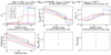 |
Fig. D.1 Effect of the magnetic field strength on the equilibrium solution when exploring weaker and stronger scenarios compared to the optimal field. Various constant mid-plane β-plasma parameters, βmid, were considered such that βmid ∈{10, 102, 103, 104, 105}. The "optimal" case (green) corresponds to the field strength used for the fiducial model, namely, the field strength that is required for the MRI activity to be at the maximal efficiency as permitted by Ohmic resistivity and ambipolar diffusion. The panels show the various steady-state profiles of some key quantities, for the model parameters M⋆ = 1 M⊙, L⋆ = 2 L⊙, Mdisk= 0.05 M⋆, adust = 1 μm, fdg = 10−2, and αhydro = 10−4. Panels (a), (b), (c), (e), and (f) show the same key quantities as in Fig. 7. Panel (d): Mid-plane r.m.s. magnetic field strengths corresponding to the various βmid as well as the optimal r.m.s. magnetic field strength (green). |
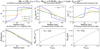 |
Fig. D.2 Effect of the hydrodynamic turbulent parameter on the equilibrium solution when varying αhydro from 10−5 to 10−3: The case αhydro = 10−5 is shown in blue, αhydro = 10−4 in dark orange (fiducial model), and αhydro = 10−3 in green. The panels show the various steady-state profiles of some key quantities, for the model parameters M⋆ = 1 M⊙, L⋆ = 2 L⊙, Mdisk= 0.05 M⋆, adust = 1 μm, and fdg = 10−2. Panels (a)-(f) show the same key quantities as in Fig. 7. The dashed black line in panel (b) corresponds to a power-law fit of Σgas as a functionof distance from the star, r. The dashed black lines in panels (e) and (f) correspond to a power-law fit of Ṁacc and RDZ as a function of αhydro, respectively. |
Overall, we notice that the choice made for the gas temperature model has very little impact on the equilibrium solution. This can be simply explained by noting that the optical thick model is only 1.5 times colder than the thin model. Additionally, most of the disk parameters only weakly depend on the gas temperature profile T. For instance, the disk gas scale height scales as  , the gas-phase recombination rate scales as k ∝ T−0.69, and the rate for the adsorption rate onto the grains scales as
  . Consequently, the ionization chemistry is barely modified by the variation from optically thick to optically thin.
D.4 Combined effect of stellar properties and total disk gas mass
In Sect. 6.4 we investigated the effect of stellar properties alone by setting the total disk gas mass to Mdisk = 0.01 M⊙ (stellar-independent choice). For each star model in Table 3, we now run a simulation with a more realistic choice for the total disk gas mass relative to the stellar mass (Mdisk = 0.05 M⋆, stellar-dependent choice). The results can be seen in Fig. D.5.
The trend seen in Sect. 6.4 where high-mass and more luminous stars generate higher accretion rates still holds, whichis expected because a higher total disk gas mass has a higher gas content that can be accreted onto the central star.
The dead zone maximal radial extent now displays a different trend compared to what we saw for the effect of stellar properties alone (Sect. 6.4). Indeed, a high-mass and more luminous star has a more massive disk, hence higher gas surface densities. The effect of total disk gas mass can thus compensate for the effect of stellar properties by significantly reducing the overall ionization level, resulting in a more extended dead zone. Nonetheless, Fig. D.5(f) displays the interesting feature that the dead zone maximal radial extent (RDZ) saturates for star 4 model. This saturation can be attributed to stellar X-rays that dominates the mid-plane ionization process for stars more massive and luminous that star 4 model, as showed by Fig. D.5(c). The high stellar X-ray luminosity (LXR) produced by such stars regulates the radial extent of the dead zone. Consequently, it seems that dead zones cannot become indefinitely large for high-mass and more luminous stars. To validate this idea, we ran six additional simulations for each star model in Table 3, varying the total disk gas mass from Mdisk = 0.001 M⋆ to Mdisk = 0.10 M⋆. For all the total disk gas masses considered, we confirm that the dead zone maximal radial extent saturates for stars more massive and luminous than star 4 model. Similarly, we find that the dead zone maximal radial extent cannot become indefinitely small for stars less massive and luminous than star 2 model due their too low stellar X-ray luminosity (Fig. D.5(f) shows that the dead zone maximal radial extent is higher for star 1 than star 2 model).
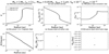 |
Fig. D.3 Effect of the gas temperature on the equilibrium solution by varying the radial profile T(r). The "optically thick" case (gray) and the "optically thin" case (black) correspond to the gas temperature profiles displayed in Fig. D.4. The optically thin case corresponds to the gas temperature profile used for the fiducial model described in Sect. 5. The panels show the various steady-state profiles of some key quantities, for the model parameters M⋆ = 1 M⊙, L⋆ = 2 L⊙, Mdisk= 0.05 M⋆, adust = 1 μm, fdg = 10−2, and αhydro = 10−4. Panels (a)-(f) show the same key quantities as in Fig. 7. |
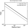 |
Fig. D.4 Gas temperature profiles for different model scenarios as a function of radius. |
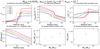 |
Fig. D.5 Combined effect of stellar properties and total disk gas mass on the equilibrium solution when varying the parameters M⋆ and L⋆ together, all the way from accreting brown dwarfs to Herbig stars. The total disk gas mass depends on the stellar mass and is such that Mdisk = 0.05 M⋆. The “star 1” case (blue) corresponds to a star of mass M⋆ = 0.05 M⊙ and bolometric luminosity L⋆ = 2 × 10⁻³ L⊙. The “star 2” case (dark orange) corresponds to a star of mass M⋆ = 0.1 M⊙ and bolometric luminosity L⋆ = 8 × 10⁻² L⊙. The “star 3” case (green) corresponds to a star of mass M⋆ = 0.3 M⊙ and bolometric luminosity L⋆ = 0.2 L⊙. The “star 4” case (red) corresponds to the fiducial model where the stellar mass is M⋆ = 1 M⊙ and the bolometric luminosity is L⋆ = 2 L⊙. The “star 5” case (purple) corresponds to a star of mass M⋆ = 2 M⊙ and bolometric luminosity L⋆ = 20 L⊙. The panels show the various steady-state profiles of some key quantities, for the model parameters Mdisk= 0.05 M⋆, adust = 1 μm, fdg = 10−2, and αhydro = 10−4. Panels (a)-(f) show the same key quantities as in Fig. 7. |
Appendix E Ambipolar diffusion and the Hall effect
In this appendix, we show that the strong-coupling limit holds in our disk models, which is a requirement for the criterion employed todescribe the effect of ambipolar diffusion on the MRI (Appendix E.1). Furthermore, we discuss the potential impact that the Hall effect could have on our steady-state accretion solutions (Appendix E.2).
E.1 Ambipolar diffusion in the strong-coupling limit
In our study we employ the Bai & Stone (2011) criterion to account for the effect of ambipolar diffusion on the MRI (see Eqs. (31) and (32)). The underlying idea behind this criterion is that the disk is in the strong-coupling limit (Shu 1991) (i.e., the single fluid regime of neutrals). In this limit, local ionization equilibrium is a good enough approximation, and the magnetic diffusion coefficients can be directly evaluated from the total ionization rate and local thermodynamic quantities such as density and temperature. It requires that: (1) the ion inertia is negligible compared to the inertia of the neutrals, so that the ion density is entirely controlled by ionization equilibrium with the neutrals; (2) the ionization equilibrium is achieved on a timescale trcb shorter than the dynamical timescale  , implying that the ions are continuously created and destroyed on a timescale that is shorter than the timescale for the MRI to grow.
It is clear that the ionization fraction is extremely small in our protoplanetary disk models, and even so in the uppermost layers (see, e.g., Fig. 4(b)). Hence, the inertia of charged particles is negligible compared to the inertia of neutrals, justifying the first requirement of the strong-coupling limit.
Since we directly solve for the equilibrium ionization state, we do not have access to the recombination timescale trcb. Nonetheless, we can estimate it as follows: Given the first term of Eqs. (A.1) and (A.2), the ionization timescale for ions and free electrons can be respectively written as  and
and  . Since ni ≥ ne (free electrons collide more frequently with grains), ti ≥ te, and hence the overall relaxation timescale of the gas-phase being given by ti. Assuming local ionization–recombination equilibrium (as it is the case in our semi-analytical chemical model), the ionization timescale (ti) equals the recombination timescale (trcb). Therefore,
  , where the second equality is found by equating Eq. (A.1) to zero. Figure E.1shows, for the fiducial model, that the recombination timescale is shorter than the dynamical timescale (trcb∕tdyn < 1) everywhere. As a result, the second requirement of the strong-coupling limit is also justified.
We can thus conclude that the strong-coupling limit holds in our fiducial disk model, justifying our use of the Bai & Stone (2011) criterion to describe the effect of ambipolar diffusion on the MRI. We verified that it holds for all the models shown in this present work.
E.2 The Hall effect
The impact of the Hall effect on the MRI is nontrivial. In the presence of a net background vertical magnetic field threading the protoplanetary disk, the non-dissipative character of Hall diffusion implies that the Hall effect depends on whether thefield is aligned or anti-aligned with the rotation axis of the disk (see, e.g., Wardle 1999; Balbus & Terquem 2001; Sano & Stone 2002a; Wardle & Salmeron 2012; Xu & Bai 2016). In Sect. 5.1, we saw that the Hall effect dominates the nonideal MHD terms in most of the dead zone, as well as in the inner regions of the MRI-active layer (Fig. 1(b)). Although we have ignored the Hall effect in our study, we can investigate a posteriori its potential impact on our results by plotting the Hall Elsasser number  (see Fig. E.2), where ηH is the Hall magnetic diffusivity (see, e.g., Wardle 2007, their Eq. (30)).
If the magnetic field is anti-aligned with the rotation axis of the disk, the Hall effect could substantially reduce the amount of MRI-driven turbulent transport in the MRI-active layer where it dominates the nonideal MHD terms (see, e.g., Kunz & Lesur 2013; Bai 2014, 2015; Simon et al. 2015). In the fiducial model, the MRI at the mid-plane would thus only develop from ≈ 50 au instead of ≈ 23 au, implying that a significant part of the mid-plane would be laminar driven by non-MRI stresses. A laminar mid-plane would have significant impact on the dust dynamics and the growth process, since lower turbulence implies effective coagulation and less effective fragmentation. It would suggest that the dust at the mid-plane could grow to larger sizes, where the typical grain size reached at agiven location in the disk would depend on how much the MRI is suppressed by the Hall effect, as well as how strong the turbulence from non-MRI stresses is.
Conversely, if the magnetic field is aligned with the rotation axis of the protoplanetary disk, the HSI could reactivate the dead zone by producing large-scale and ordered magnetic fields transporting angular momentum radially with little turbulent motion through laminar viscous stresses (see, e.g., Kunz 2008; Lesur et al. 2014; Bai 2015). As such, the steady-statepressure maximum at the dead zone outer edge seen in Sect. 6.3.2 could thus be removed.
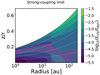 |
Fig. E.1 Ratio of the recombination timescale (trcb) to the dynamical timescale (tdyn), as a function of location in the disk, for the fiducial model described in Sect. 5. The pink hatched area corresponds to the MRI-active layer. The dashed white lines correspond to the surfaces z = 1 Hgas, z = 2 Hgas, z = 3 Hgas, and z = 4 Hgas, from bottom to top, respectively. |
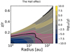 |
Fig. E.2 Steady-state Hall Elsasser number, as a function of location in the disk, for the fiducial model described in Sect. 5. The pink hatched area corresponds to the MRI-active layer. The solid black lines indicate where χ = 1. Everywhere between these lines, χ > 1. The dashed white lines correspond to the surfaces z = 1 Hgas, z = 2 Hgas, z = 3 Hgas, and z = 4 Hgas, from bottom to top, respectively. |
Appendix F Additional plots
In this section we present additional plots for completeness.
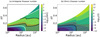 |
Fig. F.1 Steady-state ambipolar and Ohmic Elsasser numbers, as a function of location in the disk, for the fiducial model described in Sect. 5. In both panels, the red hatched area corresponds to the MRI-active layer. Additionally, the dashed white lines correspond to the surfaces z = 1 Hgas, z = 2 Hgas, z = 3 Hgas, and z = 4 Hgas, from bottomto top, respectively. Panel (a): Ambipolar Elsasser number, Am. The region within the solid white lines indicates where Am ≥ 0.1. The region within the solid black contour indicates where Am ≥ 1. Panel (b): Ohmic Elsasser number, Λ. The solid black line indicates where Λ = 1. |
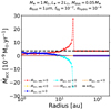 |
Fig. F.2 Accretion rates within the individual layers, as a function of radius, for the fiducial model described in Sect. 5. The overall steady-state inward accretion rate, Ṁacc, is defined as Ṁacc = Ṁacc, MRI + Ṁacc, AD + Ṁacc, DZ, where Ṁacc, MRI, Ṁacc, AD, and Ṁacc, DZ correspond to the radially variable accretion rates within the MRI-active layer, zombie zone, and dead zone, respectively. They were computed using the formula provided in Appendix B of Mohanty et al. (2018). The dashed black line corresponds to Ṁacc ≈ 3.7 × 10⁻⁹ M⊙.yr−1, obtained forthe fiducial protoplanetary disk model. |
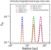 |
Fig. F.3 Vertically integrated dust-to-gas mass ratio profiles for different dust trapping scenarios as a function of radius. |
References
- ALMA Partnership (Brogan, C. L., et al.) 2015, ApJ, 808, L3 [Google Scholar]
- Anders, E., & Grevesse, N. 1989, Geochim. Cosmochim. Acta, 53, 197 [Google Scholar]
- Andrews, S. M., Wilner, D. J., Zhu, Z., et al. 2016, ApJ, 820, L40 [Google Scholar]
- Armitage, P. J. 2011, ARA&A, 49, 195 [Google Scholar]
- Armitage, P. J. 2019, Saas-Fee Advanced Course, 45, 1 [NASA ADS] [CrossRef] [Google Scholar]
- Asensio-Torres, R., Henning, T., Cantalloube, F., et al. 2021, Perturbers: SPHERE detection limits to planetary-mass companions in protoplanetary disks [Google Scholar]
- Astropy Collaboration, (Robitaille, T. P., et al.) 2013, A&A, 558, A33 [NASA ADS] [CrossRef] [EDP Sciences] [Google Scholar]
- Ataiee, S., Pinilla, P., Zsom, A., et al. 2013, A&A, 553, L3 [NASA ADS] [CrossRef] [EDP Sciences] [Google Scholar]
- Bai, X.-N. 2011, ApJ, 739, 50 [CrossRef] [Google Scholar]
- Bai, X.-N. 2014, ApJ, 791, 137 [Google Scholar]
- Bai, X.-N. 2015, ApJ, 798, 84 [Google Scholar]
- Bai, X.-N. 2016, ApJ, 821, 80 [Google Scholar]
- Bai, X.-N., & Goodman, J. 2009, ApJ, 701, 737 [NASA ADS] [CrossRef] [Google Scholar]
- Bai, X.-N., & Stone, J. M. 2011, ApJ, 736, 144 [Google Scholar]
- Bai, X.-N., & Stone, J. M. 2013, ApJ, 769, 76 [Google Scholar]
- Bai, X.-N., & Stone, J. M. 2017, ApJ, 836, 46 [Google Scholar]
- Bai, X.-N., Ye, J., Goodman, J., & Yuan, F. 2016, ApJ, 818, 152 [Google Scholar]
- Balbus, S. A., & Hawley, J. F. 1991, ApJ, 376, 214 [Google Scholar]
- Balbus, S. A., & Hawley, J. F. 1998, Rev. Mod. Phys., 70, 1 [Google Scholar]
- Balbus, S. A., & Terquem, C. 2001, ApJ, 552, 235 [NASA ADS] [CrossRef] [Google Scholar]
- Barraza-Alfaro, M., Flock, M., Marino, S., & Pérez, S. 2021, A&A 653, A113 [NASA ADS] [CrossRef] [EDP Sciences] [Google Scholar]
- Beck, R., & Hoernes, P. 1996, Nature, 379, 47 [NASA ADS] [CrossRef] [Google Scholar]
- Béthune, W., Latter, H., & Kley, W. 2021, A&A, 650, A49 [NASA ADS] [CrossRef] [EDP Sciences] [Google Scholar]
- Birnstiel, T., Dullemond, C. P., & Brauer, F. 2010, A&A, 513, A79 [NASA ADS] [CrossRef] [EDP Sciences] [Google Scholar]
- Birnstiel, T., Fang, M., & Johansen, A. 2016, Space Sci. Rev., 205, 41 [Google Scholar]
- Blandford, R. D., & Payne, D. G. 1982, MNRAS, 199, 883 [CrossRef] [Google Scholar]
- Brauer, F., Henning, T., & Dullemond, C. P. 2008, A&A, 487, L1 [NASA ADS] [CrossRef] [EDP Sciences] [Google Scholar]
- Christiaens, V., Cantalloube, F., Casassus, S., et al. 2019, ApJ, 877, L33 [Google Scholar]
- Cleeves, L. I., Adams, F. C., & Bergin, E. A. 2013a, ApJ, 772, 5 [Google Scholar]
- Cleeves, L. I., Adams, F. C., Bergin, E. A., & Visser, R. 2013b, ApJ, 777, 28 [NASA ADS] [CrossRef] [Google Scholar]
- Cui, C., & Bai, X.-N. 2021, MNRAS, 507, 1106 [NASA ADS] [CrossRef] [Google Scholar]
- D’Alessio, P., Cantó, J., Calvet, N., & Lizano, S. 1998, ApJ, 500, 411 [CrossRef] [Google Scholar]
- D’Alessio, P., Calvet, N., Hartmann, L., Lizano, S., & Cantó, J. 1999, ApJ, 527, 893 [CrossRef] [Google Scholar]
- de Boer, J., Salter, G., Benisty, M., et al. 2016, A&A, 595, A114 [NASA ADS] [CrossRef] [EDP Sciences] [Google Scholar]
- de Juan Ovelar, M., Min, M., Dominik, C., et al. 2013, A&A, 560, A111 [NASA ADS] [CrossRef] [EDP Sciences] [Google Scholar]
- Dong, R., Zhu, Z., Rafikov, R. R., & Stone, J. M. 2015, ApJ, 809, L5 [Google Scholar]
- Draine, B. T. 2011, Physics of the Interstellar and Intergalactic Medium [Google Scholar]
- Draine, B. T.,& Sutin, B. 1987, ApJ, 320, 803 [NASA ADS] [CrossRef] [Google Scholar]
- Drążkowska, J., Windmark, F., & Dullemond, C. P. 2013, A&A, 556, A37 [NASA ADS] [CrossRef] [EDP Sciences] [Google Scholar]
- Dubrulle, B., Morfill, G., & Sterzik, M. 1995, Icarus, 114, 237 [Google Scholar]
- Dullemond, C. P., & Dominik, C. 2005, A&A, 434, 971 [NASA ADS] [CrossRef] [EDP Sciences] [Google Scholar]
- Dzyurkevich, N., Flock, M., Turner, N. J., Klahr, H., & Henning, T. 2010, A&A, 515, A70 [NASA ADS] [CrossRef] [EDP Sciences] [Google Scholar]
- Dzyurkevich, N., Turner, N. J., Henning, T., & Kley, W. 2013, ApJ, 765, 114 [NASA ADS] [CrossRef] [Google Scholar]
- Fleming, T., & Stone, J. M. 2003, ApJ, 585, 908 [NASA ADS] [CrossRef] [Google Scholar]
- Fleming, T. P., Stone, J. M., & Hawley, J. F. 2000, ApJ, 530, 464 [Google Scholar]
- Flock, M., Dzyurkevich, N., Klahr, H., Turner, N. J., & Henning, T. 2011, ApJ, 735, 122 [NASA ADS] [CrossRef] [Google Scholar]
- Flock, M., Henning, T., & Klahr, H. 2012, ApJ, 761, 95 [Google Scholar]
- Flock, M., Ruge, J. P., Dzyurkevich, N., et al. 2015, A&A, 574, A68 [NASA ADS] [CrossRef] [EDP Sciences] [Google Scholar]
- Flock, M., Turner, N. J., Nelson, R. P., et al. 2020, ApJ, 897, 155 [Google Scholar]
- Fromang, S., & Nelson, R. P. 2009, A&A, 496, 597 [NASA ADS] [CrossRef] [EDP Sciences] [Google Scholar]
- Fromang, S., & Papaloizou, J. 2006, A&A, 452, 751 [NASA ADS] [CrossRef] [EDP Sciences] [Google Scholar]
- Gammie, C. F. 1996, ApJ, 457, 355 [Google Scholar]
- Gárate, M., Delage, T. N., Stadler, J., et al. 2021, A&A, 655, A18 [NASA ADS] [CrossRef] [EDP Sciences] [Google Scholar]
- Ginski, C., Stolker, T., Pinilla, P., et al. 2016, A&A, 595, A112 [NASA ADS] [CrossRef] [EDP Sciences] [Google Scholar]
- Güdel, M., Briggs, K. R., Arzner, K., et al. 2007, A&A, 468, 353 [Google Scholar]
- Guilet, J., & Ogilvie, G. I. 2014, MNRAS, 441, 852 [NASA ADS] [CrossRef] [Google Scholar]
- Haisch, Karl E., J., Lada, E. A., & Lada, C. J. 2001, ApJ, 553, L153 [Google Scholar]
- Harris, C. R., Millman, K. J., van der Walt, S. J., et al. 2020, Nature, 585, 357 [NASA ADS] [CrossRef] [Google Scholar]
- Hartmann, L., Calvet, N., Gullbring, E., & D’Alessio, P. 1998, ApJ, 495, 385 [Google Scholar]
- Hartmann, L., Herczeg, G., & Calvet, N. 2016, ARA&A, 54, 135 [Google Scholar]
- Hasegawa, Y., Okuzumi, S., Flock, M., & Turner, N. J. 2017, ApJ, 845, 31 [NASA ADS] [CrossRef] [Google Scholar]
- Hawley, J. F., Gammie, C. F., & Balbus, S. A. 1995, ApJ, 440, 742 [Google Scholar]
- Hirose, S., & Turner, N. J. 2011, ApJ, 732, L30 [NASA ADS] [CrossRef] [Google Scholar]
- Hunter, J. D. 2007, Comput. Sci. Eng., 9, 90 [NASA ADS] [CrossRef] [Google Scholar]
- Igea, J., & Glassgold, A. E. 1999, ApJ, 518, 848 [Google Scholar]
- Ilgner, M., & Nelson, R. P. 2006, A&A, 445, 223 [CrossRef] [EDP Sciences] [Google Scholar]
- Inutsuka, S.-i., & Sano, T. 2005, ApJ, 628, L155 [NASA ADS] [CrossRef] [Google Scholar]
- Isella, A., & Turner, N. 2016, ArXiv e-prints, [arXiv:1608.05123] [Google Scholar]
- Jankovic, M. R., Owen, J. E., Mohanty, S., & Tan, J. C. 2021, MNRAS, 504, 280 [NASA ADS] [CrossRef] [Google Scholar]
- Keppler, M., Benisty, M., M’́oller, A., et al. 2018, A&A, 617, A44 [NASA ADS] [CrossRef] [EDP Sciences] [Google Scholar]
- Klahr, H. H., & Bodenheimer, P. 2003, ApJ, 582, 869 [NASA ADS] [CrossRef] [Google Scholar]
- Kretke, K. A., & Lin, D. N. C. 2007, ApJ, 664, L55 [CrossRef] [Google Scholar]
- Kretke, K. A., & Lin, D. N. C. 2010, ApJ, 721, 1585 [NASA ADS] [CrossRef] [Google Scholar]
- Kretke, K. A., Lin, D. N. C., Garaud, P., & Turner, N. J. 2009, ApJ, 690, 407 [NASA ADS] [CrossRef] [Google Scholar]
- Krijt, S., & Ciesla, F. J. 2016, ApJ, 822, 111 [NASA ADS] [CrossRef] [Google Scholar]
- Kunitomo, M., Ida, S., Takeuchi, T., et al. 2021, ApJ, 909, 109 [NASA ADS] [CrossRef] [Google Scholar]
- Kunz, M. W. 2008, MNRAS, 385, 1494 [NASA ADS] [CrossRef] [Google Scholar]
- Kunz, M. W.,& Lesur, G. 2013, MNRAS, 434, 2295 [NASA ADS] [CrossRef] [Google Scholar]
- Kurtovic, N. T., Pinilla, P., Long, F., et al. 2021, A&A, 645, A139 [EDP Sciences] [Google Scholar]
- Lesur, G. R. J. 2021, A&A, 650, A35 [NASA ADS] [CrossRef] [EDP Sciences] [Google Scholar]
- Lesur, G., Kunz, M. W., & Fromang, S. 2014, A&A, 566, A56 [NASA ADS] [CrossRef] [EDP Sciences] [Google Scholar]
- Lin, D. N. C.,& Pringle, J. E. 1987, MNRAS, 225, 607 [NASA ADS] [CrossRef] [Google Scholar]
- Lin, M.-K., & Youdin, A. N. 2015, ApJ, 811, 17 [NASA ADS] [CrossRef] [Google Scholar]
- Lodato, G., & Rice, W. K. M. 2004, MNRAS, 351, 630 [Google Scholar]
- Lubow, S. H., Papaloizou, J. C. B., & Pringle, J. E. 1994, MNRAS, 267, 235 [NASA ADS] [Google Scholar]
- Lynden-Bell, D., & Pringle, J. E. 1974, MNRAS, 168, 603 [Google Scholar]
- Manara, C. F., Testi, L., Herczeg, G. J., et al. 2017, A&A, 604, A127 [NASA ADS] [CrossRef] [EDP Sciences] [Google Scholar]
- Manger, N., Klahr, H., Kley, W., & Flock, M. 2020, MNRAS, 499, 1841 [NASA ADS] [CrossRef] [Google Scholar]
- McCall, B. J., Huneycutt, A. J., Saykally, R. J., et al. 2003, Nature, 422, 500 [CrossRef] [Google Scholar]
- McElroy, D., Walsh, C., Markwick, A. J., et al. 2013, A&A, 550, A36 [NASA ADS] [CrossRef] [EDP Sciences] [Google Scholar]
- Miller, K. A., & Stone, J. M. 2000, ApJ, 534, 398 [NASA ADS] [CrossRef] [Google Scholar]
- Mohanty, S., Ercolano, B., & Turner, N. J. 2013a, ApJ, 764, 65 [NASA ADS] [CrossRef] [Google Scholar]
- Mohanty, S., Greaves, J., Mortlock, D., et al. 2013b, ApJ, 773, 168 [NASA ADS] [CrossRef] [Google Scholar]
- Mohanty, S., Jankovic, M. R., Tan, J. C., & Owen, J. E. 2018, ApJ, 861, 144 [Google Scholar]
- Mori, S., Bai, X.-N., & Okuzumi, S. 2019, ApJ, 872, 98 [NASA ADS] [CrossRef] [Google Scholar]
- Mori, S., Okuzumi, S., Kunitomo, M., & Bai, X.-N. 2021, ApJ, 916, 72 [NASA ADS] [CrossRef] [Google Scholar]
- Nakagawa, Y., Nakazawa, K., & Hayashi, C. 1981, Icarus, 45, 517 [NASA ADS] [CrossRef] [Google Scholar]
- Nelson, R. P., Gressel, O., & Umurhan, O. M. 2013, MNRAS, 435, 2610 [Google Scholar]
- Nishi, R., Nakano, T., & Umebayashi, T. 1991, ApJ, 368, 181 [NASA ADS] [CrossRef] [Google Scholar]
- Nomura, H., Tsukagoshi, T., Kawabe, R., et al. 2016, ApJ, 819, L7 [Google Scholar]
- Oishi, J. S., & Mac Low, M.-M. 2009, ApJ, 704, 1239 [NASA ADS] [CrossRef] [Google Scholar]
- Okuzumi, S. 2009, ApJ, 698, 1122 [Google Scholar]
- Okuzumi, S., & Hirose, S. 2011, ApJ, 742, 65 [NASA ADS] [CrossRef] [Google Scholar]
- Okuzumi, S., & Hirose, S. 2012, ApJ, 753, L8 [CrossRef] [Google Scholar]
- Okuzumi, S., Takeuchi, T., & Muto, T. 2014, ApJ, 785, 127 [NASA ADS] [CrossRef] [Google Scholar]
- Oppenheimer, M., & Dalgarno, A. 1974, ApJ, 192, 29 [NASA ADS] [CrossRef] [Google Scholar]
- Ormel, C. W., & Okuzumi, S. 2013, ApJ, 771, 44 [NASA ADS] [CrossRef] [Google Scholar]
- Owen, J. E., & Kollmeier, J. A. 2019, MNRAS, 487, 3702 [Google Scholar]
- Parkin, E. R., & Bicknell, G. V. 2013a, ApJ, 763, 99 [CrossRef] [Google Scholar]
- Parkin, E. R., & Bicknell, G. V. 2013b, MNRAS, 435, 2281 [NASA ADS] [CrossRef] [Google Scholar]
- Pascucci, I., Testi, L., Herczeg, G. J., et al. 2016, ApJ, 831, 125 [Google Scholar]
- Pérez, L. M., Carpenter, J. M., Andrews, S. M., et al. 2016, Science, 353, 1519 [Google Scholar]
- Perez-Becker, D., & Chiang, E. 2011, ApJ, 735, 8 [Google Scholar]
- Pessah, M. E. 2010, ApJ, 716, 1012 [NASA ADS] [CrossRef] [Google Scholar]
- Pinilla, P., & Youdin, A. 2017, Particle Trapping in Protoplanetary Disks: Models vs. Observations, 445, eds. M. Pessah, & O. Gressel, 91 [Google Scholar]
- Pinilla, P., Benisty, M., & Birnstiel, T. 2012, A&A, 545, A81 [NASA ADS] [CrossRef] [EDP Sciences] [Google Scholar]
- Pinilla, P., de Juan Ovelar, M., Ataiee, S., et al. 2015, A&A, 573, A9 [NASA ADS] [CrossRef] [EDP Sciences] [Google Scholar]
- Pinilla, P., Flock, M., Ovelar, M. d. J., & Birnstiel, T. 2016, A&A, 596, A81 [NASA ADS] [CrossRef] [EDP Sciences] [Google Scholar]
- Pinte, C., Padgett, D. L., Ménard, F., et al. 2008, A&A, 489, 633 [NASA ADS] [CrossRef] [EDP Sciences] [Google Scholar]
- Pohl, A., Pinilla, P., Benisty, M., et al. 2015, MNRAS, 453, 1768 [NASA ADS] [CrossRef] [Google Scholar]
- Pollack, J. B., Hollenbach, D., Beckwith, S., et al. 1994, ApJ, 421, 615 [Google Scholar]
- Rab, C., Güdel, M., Padovani, M., et al. 2017, A&A, 603, A96 [NASA ADS] [CrossRef] [EDP Sciences] [Google Scholar]
- Raettig, N., Lyra, W., & Klahr, H. 2013, ApJ, 765, 115 [Google Scholar]
- Sano, T., & Miyama, S. M. 1999, ApJ, 515, 776 [CrossRef] [Google Scholar]
- Sano, T., & Stone, J. M. 2002a, ApJ, 570, 314 [NASA ADS] [CrossRef] [Google Scholar]
- Sano, T., & Stone, J. M. 2002b, ApJ, 577, 534 [NASA ADS] [CrossRef] [Google Scholar]
- Sano, T., Inutsuka, S.-i., Turner, N. J., & Stone, J. M. 2004, ApJ, 605, 321 [NASA ADS] [CrossRef] [Google Scholar]
- Scholz, A., Jayawardhana, R., & Wood, K. 2006, ApJ, 645, 1498 [NASA ADS] [CrossRef] [Google Scholar]
- Semenov, D., Wiebe, D., & Henning, T. 2004, A&A, 417, 93 [NASA ADS] [CrossRef] [EDP Sciences] [Google Scholar]
- Shakura, N. I., & Sunyaev, R. A. 1973, A&A, 500, 33 [NASA ADS] [Google Scholar]
- Shu, F. 1991, Physics of Astrophysics, Vol. II: Gas Dynamics [Google Scholar]
- Simon, J. B., Hawley, J. F., & Beckwith, K. 2011, ApJ, 730, 94 [NASA ADS] [CrossRef] [Google Scholar]
- Simon, J. B., Bai, X.-N., Armitage, P. J., Stone, J. M., & Beckwith, K. 2013a, ApJ, 775, 73 [NASA ADS] [CrossRef] [Google Scholar]
- Simon, J. B., Bai, X.-N., Stone, J. M., Armitage, P. J., & Beckwith, K. 2013b, ApJ, 764, 66 [NASA ADS] [CrossRef] [Google Scholar]
- Simon, J. B., Lesur, G., Kunz, M. W., & Armitage, P. J. 2015, MNRAS, 454, 1117 [NASA ADS] [CrossRef] [Google Scholar]
- Suriano, S. S., Li, Z.-Y., Krasnopolsky, R., & Shang, H. 2017, MNRAS, 468, 3850 [NASA ADS] [CrossRef] [Google Scholar]
- Suriano, S. S., Li, Z.-Y., Krasnopolsky, R., & Shang, H. 2018, MNRAS, 477, 1239 [NASA ADS] [CrossRef] [Google Scholar]
- Suriano, S. S., Li, Z.-Y., Krasnopolsky, R., Suzuki, T. K., & Shang, H. 2019, MNRAS, 484, 107 [NASA ADS] [CrossRef] [Google Scholar]
- Suzuki, T. K.,& Inutsuka, S.-i. 2009, ApJ, 691, L49 [NASA ADS] [CrossRef] [Google Scholar]
- Suzuki, T. K., Muto, T., & Inutsuka, S.-i. 2010, ApJ, 718, 1289 [NASA ADS] [CrossRef] [Google Scholar]
- Takeuchi, T., & Okuzumi, S. 2014, ApJ, 797, 132 [CrossRef] [Google Scholar]
- Teague, R., Bae, J., Bergin, E. A., Birnstiel, T., & Foreman-Mackey, D. 2018, ApJ, 860, L12 [NASA ADS] [CrossRef] [Google Scholar]
- Teague, R., Bae, J., & Bergin, E. A. 2019, Nature, 574, 378 [NASA ADS] [CrossRef] [Google Scholar]
- Terquem, C. E. J. M. L. J. 2008, ApJ, 689, 532 [NASA ADS] [CrossRef] [Google Scholar]
- Toomre, A. 1964, ApJ, 139, 1217 [Google Scholar]
- Turner, N. J., & Sano, T. 2008, ApJ, 679, L131 [Google Scholar]
- Turner, N. J., Sano, T., & Dziourkevitch, N. 2007, ApJ, 659, 729 [NASA ADS] [CrossRef] [Google Scholar]
- Turner, N. J., Carballido, A., & Sano, T. 2010, ApJ, 708, 188 [CrossRef] [Google Scholar]
- Umebayashi, T., & Nakano, T. 1980, PASJ, 32, 405 [NASA ADS] [Google Scholar]
- Umebayashi, T., & Nakano, T. 1990, MNRAS, 243, 103 [NASA ADS] [CrossRef] [Google Scholar]
- Umebayashi, T., & Nakano, T. 2009, ApJ, 690, 69 [Google Scholar]
- Urpin, V., & Brandenburg, A. 1998, MNRAS, 294, 399 [Google Scholar]
- van der Marel,N., & Mulders, G. 2021, AJ, 162, 28 [NASA ADS] [CrossRef] [Google Scholar]
- Varnière, P., & Tagger, M. 2006, A&A, 446, L13 [NASA ADS] [CrossRef] [EDP Sciences] [Google Scholar]
- Villenave, M., Benisty, M., Dent, W. R. F., et al. 2019, A&A, 624, A7 [NASA ADS] [CrossRef] [EDP Sciences] [Google Scholar]
- Villenave, M., Ménard, F., Dent, W. R. F., et al. 2020, A&A, 642, A164 [EDP Sciences] [Google Scholar]
- Virtanen, P., Gommers, R., Oliphant, T. E., et al. 2020, Nat. Methods, 17, 261 [Google Scholar]
- Vorobyov, E. I., & Basu, S. 2009, MNRAS, 393, 822–837 [CrossRef] [Google Scholar]
- Wardle, M. 1999, MNRAS, 307, 849 [NASA ADS] [CrossRef] [Google Scholar]
- Wardle, M. 2007, Ap&SS, 311, 35 [NASA ADS] [CrossRef] [Google Scholar]
- Wardle, M., & Ng, C. 1999, MNRAS, 303, 239 [NASA ADS] [CrossRef] [Google Scholar]
- Wardle, M., & Salmeron, R. 2012, MNRAS, 422, 2737 [NASA ADS] [CrossRef] [Google Scholar]
- Weidenschilling, S. J. 1977, MNRAS, 180, 57 [Google Scholar]
- Xu, R., & Bai, X.-N. 2016, ApJ, 819, 68 [NASA ADS] [CrossRef] [Google Scholar]
- Yang, C.-C., & Menou, K. 2010, MNRAS, 402, 2436 [NASA ADS] [CrossRef] [Google Scholar]
- Zhu, Z., & Stone, J. M. 2018, ApJ, 857, 34 [Google Scholar]
- Zhu, Z., Nelson, R. P., Dong, R., Espaillat, C., & Hartmann, L. 2012, ApJ, 755, 6 [Google Scholar]
We emphasize that our framework can also be used with, e.g., the self-similar solution (Lynden-Bell & Pringle 1974) as for the gas surface density. In this case, though, the derived accretion rate would be radially variable, implying that some regions of the disk can accrete more than others. This scenario would thus not describe a steady-state accretion state for the disk.
For instance, the self-similar α-constant disk model has a gas mass distribution given by M<(r) = Mtot,self-similar[1 − exp(−r∕(2Rt))], where M<(r) is the disk gas mass within disk radius, r, and Mtot,self-similar is the total gas mass of the whole self-similar disk (see, e.g., Hartmann et al. 1998). For this specific model, the inner inward-accreting region (r ≲ Rt) comprises ≈40% of the total disk gas mass. Neglecting the gas mass within the outer viscously expanding region (r ≳ Rt) thus underestimates the total disk gas mass by only ≈60%.
All Tables
Summary of the viscous formation timescales for the potential steady-state pressure maxima formed by local dust enhancement at various locations in the protoplanetary disk.
Summary of the stellar parameters (mass, M⋆, and luminosity, L⋆) used to investigate the effect of stellar properties on the equilibrium solution.
All Figures
|
Fig. 1 Panel a: steady-state accretion layers, as a function of location in the disk, for the fiducial model. The black colored area corresponds to the dead zone. The gray colored area corresponds to the zombie zone. The red and black hatched area corresponds to the MRI-active layer. The region within the dash-dotted magenta lines defines where the ambipolar condition (β > βmin) is satisfied in the disk, while the region above the dashed cyan line defines where the Ohmic condition (Λ > 1) is fulfilled. The region above the solid green line corresponds to where β > 1. The dashed white lines correspond to the surfaces z = 1 Hgas, z = 2 Hgas, z = 3 Hgas, and z = 4 Hgas, from bottom to top, respectively. Panel b: Regimes of the nonideal MHD effects by showing the dominant magnetic diffusivities as a function of location in the disk. In the orange colored region the Ohmic resistivity dominates (ηO is the highest magnetic diffusivity), in the gray and blue colored regions the Hall effect dominates (|ηH | is the highest magnetic diffusivity), and in the green colored regions ambipolar diffusion dominates (ηAD is the highest magnetic diffusivity). The MRI-active layer is shown by the black hatched area. The dashed white lines are the same as in panel a. |
| In the text | |
|
Fig. 2 Steady-state gas surface density, Σgas (Eq. (42)), as a function of radius, for the fiducial model. The dashed gray line shows the initial gas surface density by initially assuming that the effective turbulent parameter,
|
| In the text | |
|
Fig. 3 Steady-state ionization rates for the fiducial model. The total ionization rate for H2 (ζ(H2); solid black line) is the sum of the following contributions: the radionuclides ionization rate for H2 ( |
| In the text | |
|
Fig. 4 Steady-state ionization fraction, xe (ne is defined by Eq. (24)), for the fiducial model. Panel a: mid-plane ionization fraction as a function of radius. The gray shaded area corresponds to the radial locations within the mid-plane dead zone. Panel b: vertical profiles for the ionization fraction at the same radial locations as in Fig. 3. The solid black line corresponds to r = 1 au. The solid red line corresponds to r = 23− au. The solid blue line corresponds to r = 23+ au. The solid green line corresponds to r = 80 au. |
| In the text | |
|
Fig. 5 Steady-state quantities describing the disk magnetization for the fiducial model. Panel a: mid-plane magnetic fields strength as a function of radius. The solid black line corresponds to B, the optimalr.m.s. magnetic field strength that is required for the MRI activity to be at the maximal efficiency as permitted by Ohmic resistivity and ambipolar diffusion (Sect. 3.2). The dotted red line corresponds to
|
| In the text | |
|
Fig. 6 Steady-state quantities describing the turbulence state in the disk for the fiducial model. Panel a: local turbulence parameter, α (Eq. (40)), as a function of location in the disk. The region above the solid red line corresponds to where β > 1. The dashed white lines correspond to the surfaces z = 1 Hgas, z = 2 Hgas, z = 3 Hgas, and z = 4 Hgas, from bottom to top, respectively. Panel b: vertical profiles for the local turbulent parameter, α, at various radial locations, with color codes as in Fig. 4. Panel c: MRI-active layer thickness, hMRI, as a function of radius, expressed in terms of the disk gas scale height, Hgas. Panel d: pressure-weighted vertically integrated turbulent parameter, |
| In the text | |
|
Fig. 7 Effect of the total disk gas mass on the equilibrium solution when varying the parameter Mdisk from 0.005 M⋆ (gas-poor disk) to 0.10 M⋆ (gas-rich disk close to the GI limit): The case Mdisk = 0.005 M⋆ is shown in blue, Mdisk = 0.01 M⋆ in dark orange, Mdisk = 0.05 M⋆ in green (fiducial model), and Mdisk = 0.10 M⋆ in red. The panels show the various steady-state profiles of some key quantities, for the model parameters M⋆ = 1 M⊙, L⋆ = 2 L⊙, adust =1 μm, fdg = 10−2, and αhydro = 10−4. Panel a: pressure-weighted vertically integrated turbulent parameter, |
| In the text | |
|
Fig. 8 Effect of the grain size on the equilibrium solution when varying the parameter adust from 0.1 μm to 1 mm: The case adust = 0.1 μm is shown in blue, adust = 1 μm in dark orange (fiducial model), adust = 10 μm in green, adust = 100 μm in red, and adust = 1 mm in purple. The panels show the various steady-state profiles of some key quantities, for the model parameters M⋆ = 1 M⊙, L⋆ = 2 L⊙, Mdisk = 0.05 M⋆, fdg = 10−2, and αhydro = 10−4. Panels a–f show the same key quantities as in Fig. 7. |
| In the text | |
|
Fig. 9 Effect of overall change in the vertically integrated dust-to-gas mass ratio on the equilibrium solution when varying the radially constant parameter fdg from 10−5 (99.9 dust depletion relative to standard ISM) to 10−1 (dust-rich disk): The case fdg = 10−5 is shown in blue, fdg = 10−4 in dark orange, fdg = 10−3 in green, fdg = 10−2 in red (fiducial model), and fdg = 10−1 in purple. The panels show the various steady-state profiles of some key quantities, for the model parameters M⋆ = 1 M⊙, L⋆ = 2 L⊙, Mdisk = 0.05 M⋆, adust =1 μm, and αhydro = 10−4. Panels a–f show the same key quantities as in Fig. 7. |
| In the text | |
|
Fig. 10 Effect of local enhancements in the vertically integrated dust-to-gas mass ratio on the equilibrium solution by imposing fdg to be radially variable with a local Gaussian perturbation at various locations (see the dust-to-gas mass ratio profiles in Fig. F.3). The unperturbed value of fdg is the same for all the simulations, equal to 10−2. The ”5 au (10×)” case (blue) corresponds to dust enhancement at r = 5 au, where fdg varies from its unperturbed value to 10−1. The “5 au (5×)” case (dark orange) is similar to the previous case, but fdg goes up to 5 × 10⁻² instead. The “DZOE (10×)” case (green) corresponds to dust enhancement at the expected dead zone outer edge (DZOE) location for the fiducial model (r = 23 au), where fdg varies from its unperturbed value to 10−1. The “DZOE (5×)” case (red) is similar to the previous case, but fdg goes up to 5 × 10⁻² instead. The “60 au (10×)” case (purple) corresponds to dust enhancement at r = 60 au, where fdgvaries from its unperturbed value to 10−1. The “60 au (5×)” case (brown) is similar to the previous case, but fdg goes up to 5 × 10⁻² instead. The ”No dust enhancement” case (gray) corresponds to the fiducial model. The panels show the various steady-state profiles of some key quantities, for the model parameters M⋆ = 1 M⊙, L⋆ = 2 L⊙, Mdisk = 0.05 M⋆, adust = 1 μm, and αhydro = 10−4. Panels a–e show the same key quantities as in Fig. 7. Panel f: deviation from Keplerian velocity, where vϕ, gas is the azimuthal gas velocity and vK = rΩK is the Keplerian velocity. The dotted black line corresponds to vϕ, gas = vK. |
| In the text | |
|
Fig. 11 Effect of stellar properties on the equilibrium solution when varying the parameters M⋆ and L⋆ together, all the way from accreting brown dwarfs to Herbig stars. The total disk gas mass does not depend on stellar mass and is such that Mdisk = 0.01 M⊙. The “star 1” case (blue) corresponds to a star of mass M⋆ = 0.05 M⊙ and bolometric luminosity L⋆ = 2 × 10⁻³ L⊙. The “star 2” case (dark orange) corresponds to a star of mass M⋆ = 0.1 M⊙ and bolometric luminosity L⋆ = 8 × 10⁻² L⊙. The “star 3” case (green) corresponds to a star of mass M⋆ = 0.3 M⊙ and bolometric luminosity L⋆ = 0.2 L⊙. The “star 4” case (red) corresponds to the fiducial model where the stellar mass is M⋆ = 1 M⊙ and the bolometric luminosity is L⋆ = 2 L⊙. The ”star 5” case (purple) corresponds to a star of mass M⋆ = 2 M⊙ and bolometric luminosity L⋆ = 20 L⊙. The panels show the various steady-state profiles of some key quantities, for the model parameters Mdisk = 0.05 M⋆, adust =1 μm, fdg = 10−2, and αhydro = 10−4. Panels a–f show the same key quantities as in Fig. 7. |
| In the text | |
|
Fig. 12 Various local timescales, as a function of radius, for the fiducial model described in Sect. 5. The solid blue line (tvisc) corresponds to the viscous evolution timescale. The solid orange line (tdyn) corresponds to the dynamical timescale. The solid green line (tgrowth) corresponds to the growth timescale for the case of micron-sized particles. The dashed black line corresponds to 1 Myr. |
| In the text | |
|
Fig. 13 Accretion rate as a function of stellar mass. The dash-dotted and solid black lines correspond to the single-line and segmented-line best-fit models, respectively, from Manara et al. (2017). The 1σ dispersion around the single-line best-fit model is shown by the gray area. The “+” symbols represent the accretion rates obtained for various total disk gas masses and for each star taken from Table 3, using our steady-state accretion model. Here we assume that adust =1 μm, fdg = 10−2, and αhydro = 10−4. |
| In the text | |
|
Fig. B.1 Comparison between the semi-analytical chemical model employed in this study and a chemical reaction network, for the fiducial model described in Sect. 5. The panels show various species abundances as a function of height, z, at r =5 au and r = 100 au (upper and lower rows, respectively). Left panels: Free electron abundance from the chemical reaction network (solid green lines) and the semi-analytical model (dotted black lines). Central panels: Total ion abundance from the chemical reaction network (solid green lines) and the semi-analytical model (dotted black lines). Right panels: Abundances of individual ion species from the chemical reaction network. The solid black line corresponds to HCO+, the solid blue line to H |
| In the text | |
|
Fig. C.1 Ionization rate for H2 ζ(H2) (defined in Sect. 2.3) and its different contributions, as a function of location in the disk, for the fiducial model described in Sect. 5. For each color, the following nonthermal ionization source dominates ζ(H2): decay from short- and long-lived radionuclides (black), galactic cosmic rays (purple), or stellar X-rays (orange and yellow for the scattered and direct contribution, respectively). The solid colored contour lines correspond to the surfaces of constant total ionization rate, ζ(H2), ranging from7.6 × 10−19 s−1 to 1.8 × 10⁻¹⁰ s−1. The dashed white lines correspond to the surfaces z = 1 Hgas, z = 2 Hgas, z = 3 Hgas, and z = 4 Hgas, from bottom to top, respectively. |
| In the text | |
|
Fig. D.1 Effect of the magnetic field strength on the equilibrium solution when exploring weaker and stronger scenarios compared to the optimal field. Various constant mid-plane β-plasma parameters, βmid, were considered such that βmid ∈{10, 102, 103, 104, 105}. The "optimal" case (green) corresponds to the field strength used for the fiducial model, namely, the field strength that is required for the MRI activity to be at the maximal efficiency as permitted by Ohmic resistivity and ambipolar diffusion. The panels show the various steady-state profiles of some key quantities, for the model parameters M⋆ = 1 M⊙, L⋆ = 2 L⊙, Mdisk= 0.05 M⋆, adust = 1 μm, fdg = 10−2, and αhydro = 10−4. Panels (a), (b), (c), (e), and (f) show the same key quantities as in Fig. 7. Panel (d): Mid-plane r.m.s. magnetic field strengths corresponding to the various βmid as well as the optimal r.m.s. magnetic field strength (green). |
| In the text | |
|
Fig. D.2 Effect of the hydrodynamic turbulent parameter on the equilibrium solution when varying αhydro from 10−5 to 10−3: The case αhydro = 10−5 is shown in blue, αhydro = 10−4 in dark orange (fiducial model), and αhydro = 10−3 in green. The panels show the various steady-state profiles of some key quantities, for the model parameters M⋆ = 1 M⊙, L⋆ = 2 L⊙, Mdisk= 0.05 M⋆, adust = 1 μm, and fdg = 10−2. Panels (a)-(f) show the same key quantities as in Fig. 7. The dashed black line in panel (b) corresponds to a power-law fit of Σgas as a functionof distance from the star, r. The dashed black lines in panels (e) and (f) correspond to a power-law fit of Ṁacc and RDZ as a function of αhydro, respectively. |
| In the text | |
|
Fig. D.3 Effect of the gas temperature on the equilibrium solution by varying the radial profile T(r). The "optically thick" case (gray) and the "optically thin" case (black) correspond to the gas temperature profiles displayed in Fig. D.4. The optically thin case corresponds to the gas temperature profile used for the fiducial model described in Sect. 5. The panels show the various steady-state profiles of some key quantities, for the model parameters M⋆ = 1 M⊙, L⋆ = 2 L⊙, Mdisk= 0.05 M⋆, adust = 1 μm, fdg = 10−2, and αhydro = 10−4. Panels (a)-(f) show the same key quantities as in Fig. 7. |
| In the text | |
|
Fig. D.4 Gas temperature profiles for different model scenarios as a function of radius. |
| In the text | |
|
Fig. D.5 Combined effect of stellar properties and total disk gas mass on the equilibrium solution when varying the parameters M⋆ and L⋆ together, all the way from accreting brown dwarfs to Herbig stars. The total disk gas mass depends on the stellar mass and is such that Mdisk = 0.05 M⋆. The “star 1” case (blue) corresponds to a star of mass M⋆ = 0.05 M⊙ and bolometric luminosity L⋆ = 2 × 10⁻³ L⊙. The “star 2” case (dark orange) corresponds to a star of mass M⋆ = 0.1 M⊙ and bolometric luminosity L⋆ = 8 × 10⁻² L⊙. The “star 3” case (green) corresponds to a star of mass M⋆ = 0.3 M⊙ and bolometric luminosity L⋆ = 0.2 L⊙. The “star 4” case (red) corresponds to the fiducial model where the stellar mass is M⋆ = 1 M⊙ and the bolometric luminosity is L⋆ = 2 L⊙. The “star 5” case (purple) corresponds to a star of mass M⋆ = 2 M⊙ and bolometric luminosity L⋆ = 20 L⊙. The panels show the various steady-state profiles of some key quantities, for the model parameters Mdisk= 0.05 M⋆, adust = 1 μm, fdg = 10−2, and αhydro = 10−4. Panels (a)-(f) show the same key quantities as in Fig. 7. |
| In the text | |
|
Fig. E.1 Ratio of the recombination timescale (trcb) to the dynamical timescale (tdyn), as a function of location in the disk, for the fiducial model described in Sect. 5. The pink hatched area corresponds to the MRI-active layer. The dashed white lines correspond to the surfaces z = 1 Hgas, z = 2 Hgas, z = 3 Hgas, and z = 4 Hgas, from bottom to top, respectively. |
| In the text | |
|
Fig. E.2 Steady-state Hall Elsasser number, as a function of location in the disk, for the fiducial model described in Sect. 5. The pink hatched area corresponds to the MRI-active layer. The solid black lines indicate where χ = 1. Everywhere between these lines, χ > 1. The dashed white lines correspond to the surfaces z = 1 Hgas, z = 2 Hgas, z = 3 Hgas, and z = 4 Hgas, from bottom to top, respectively. |
| In the text | |
|
Fig. F.1 Steady-state ambipolar and Ohmic Elsasser numbers, as a function of location in the disk, for the fiducial model described in Sect. 5. In both panels, the red hatched area corresponds to the MRI-active layer. Additionally, the dashed white lines correspond to the surfaces z = 1 Hgas, z = 2 Hgas, z = 3 Hgas, and z = 4 Hgas, from bottomto top, respectively. Panel (a): Ambipolar Elsasser number, Am. The region within the solid white lines indicates where Am ≥ 0.1. The region within the solid black contour indicates where Am ≥ 1. Panel (b): Ohmic Elsasser number, Λ. The solid black line indicates where Λ = 1. |
| In the text | |
|
Fig. F.2 Accretion rates within the individual layers, as a function of radius, for the fiducial model described in Sect. 5. The overall steady-state inward accretion rate, Ṁacc, is defined as Ṁacc = Ṁacc, MRI + Ṁacc, AD + Ṁacc, DZ, where Ṁacc, MRI, Ṁacc, AD, and Ṁacc, DZ correspond to the radially variable accretion rates within the MRI-active layer, zombie zone, and dead zone, respectively. They were computed using the formula provided in Appendix B of Mohanty et al. (2018). The dashed black line corresponds to Ṁacc ≈ 3.7 × 10⁻⁹ M⊙.yr−1, obtained forthe fiducial protoplanetary disk model. |
| In the text | |
|
Fig. F.3 Vertically integrated dust-to-gas mass ratio profiles for different dust trapping scenarios as a function of radius. |
| In the text | |
Current usage metrics show cumulative count of Article Views (full-text article views including HTML views, PDF and ePub downloads, according to the available data) and Abstracts Views on Vision4Press platform.
Data correspond to usage on the plateform after 2015. The current usage metrics is available 48-96 hours after online publication and is updated daily on week days.
Initial download of the metrics may take a while.