| Issue |
A&A
Volume 658, February 2022
|
|
|---|---|---|
| Article Number | A18 | |
| Number of page(s) | 10 | |
| Section | The Sun and the Heliosphere | |
| DOI | https://doi.org/10.1051/0004-6361/202040233 | |
| Published online | 25 January 2022 | |
Prominence instability and CMEs triggered by massive coronal rain in the solar atmosphere
1
IGAM, Institute of Physics, University of Graz, Universitätsplatz 5, 8010 Graz, Austria
2
Ilia State University, Kakutsa Cholokashvili Ave 3/5, 0162 Tbilisi, Georgia
e-mail: This email address is being protected from spambots. You need JavaScript enabled to view it.
3
E.Kharadze Georgian National Astrophysical Observatory, Mount Kanobili, Abastumani, Georgia
4
Astronomical Institute, Slovak Academy of Sciences, PO Box 18, 05960 Tatranská Lomnica, Slovak Republic
Received:
24
December
2020
Accepted:
28
September
2021
Abstract
Context. The triggering process for prominence instability and consequent coronal mass ejections (CMEs) is not fully understood. Prominences are maintained by the Lorentz force against the gravity; therefore, reduction of the prominence mass due to the coronal rain may cause the change of the force balance and hence destabilisation of the structures.
Aims. We aim to study the observational evidence of the influence of coronal rain on the stability of prominence and subsequent eruption of CMEs.
Methods. We used the simultaneous observations from the Atmospheric Imaging Assembly (AIA) of Solar Dynamics Observatory (SDO) and Sun Earth Connection Coronal and Heliospheric Investigation (SECHHI) of Solar Terrestrial Relations Observatory (STEREO) spacecrafts from different angles to follow the dynamics of prominence and to study the role of coronal rain in their destabilisation.
Results. Three different prominences observed during the years 2011–2012 were analysed using observations acquired by SDO and STEREO. In all three cases, massive coronal rain from the prominence body led to the destabilisation of prominence and subsequently to the eruption of CMEs. The upward rising of prominences consisted of the slow and fast rise phases. The coronal rain triggered the initial slow rise of prominences, which led to the final instability (the fast rise phase) after 18–28 h in all cases. The estimated mass flux carried by coronal rain blobs showed that the prominences became unstable after 40% of mass loss.
Conclusions. We suggest that the initial slow rise phase was triggered by the mass loss of prominence due to massive coronal rain, while the fast rise phase (the consequent instability of prominences) was caused by the torus instability and/or magnetic reconnection with the overlying coronal field. Therefore, the coronal rain triggered the instability of prominences and consequent CMEs. If this is the case, then the coronal rain can be used to predict the CMEs and hence to improve the space weather predictions.
Key words: Sun: corona / Sun: filaments, prominences / Sun: coronal mass ejections / Sun: atmosphere
© ESO 2022
1. Introduction
Solar prominences are relatively cool and dense structures in the tenuous, hot solar corona (Labrose et al. 2010; Arregui et al. 2012). Most active region prominences are relatively unstable and lead to CMEs, which affect space weather conditions near the Earth (Panesar 2014; Schmieder et al. 2002; Gopalswamy et al. 2003). Prominence instability, the initiation of CMEs (Priest & Forbes 2002), and an interconnection between CMEs and erupting prominences are not clearly understood (Chae et al. 2000; Zhang et al. 2017a; Zirker et al. 1998). Observations show that the prominences are supported by the coronal magnetic field against the gravity (Ning et al. 2009; Shen et al. 2015; Zhang et al. 2017b). Therefore, a process (or processes) must destabilise the equilibrium and lead to the prominence instability and consequently to the CME eruption.
The most acceptable triggering mechanism for the prominence instability is connected to twisted magnetic configurations. It has been observed that the kink instability of magnetic flux ropes (Williams et al. 2005), the torus instability (Filippov 2013; Zuccarello et al. 2014), or both together (Vasantharaju et al. 2019) can lead to CME initiations.
Another phenomenon in the solar atmosphere is coronal rain, which is cool and dense material condensing at solar coronal loops falling along their legs. The condensations are probably caused by thermal instability (Parker 1953; Field 1965). Another type of coronal rain is related to solar prominences, where cool blobs detach from the prominence main body and fall down towards the photosphere. Recent SDO observations show the formation of the prominence by the condensation after CME, where most of the mass drained down through vertical downward flows (Liu et al. 2012). Liu et al. (2012) concluded that these flows show up as cool and dense plasma blobs that started falling at a height between 20–40 Mm. The measurement of velocity has a narrow Gaussian distribution with values of 30 km s−1, while the derived accelerations have an average value of 46 m s−2. It was assumed that the thermal instability is responsible for the plasma condensation, and hence the coronal rain through catastrophic cooling, that is when the energy balance is violated as the radiative losses locally overcome the heating input (Parker 1953; Field 1965; Antiochos et al. 1999; Schrijver 2001; Vashalomidze et al. 2015). Numerical simulations also show that the thermal instability is the reason for the formation of cold condensation and coronal rain (Müller et al. 2003, 2004, 2005).
The equilibrium state of prominences is achieved owing to the balance between gravity and Lorentz forces (in the low-beta plasma). Massive plasma downflows from prominences in the form of coronal rain will lead to the decrease of the prominence mass, which may affect the equilibrium. The Lorentz force may succeed over gravity after some time, and the prominence may start to rise slowly. This slow rising process may trigger a magnetic reconnection and/or instability, which can lead to CMEs. In this paper, we present several pieces of observational evidence of prominence instability as triggered by massive downflows in the form of coronal rain.
2. Observation and data analysis
We used observations from SDO/AIA (Pesnell et al. 2012; Lemen et al. 2012), and SECCHI on board STEREO. SECCHI and the Extreme Ultraviolet Imager (EUVI) take images in the 304 Å, 171 Å, 195 Å, and 284 Å channels with the spatial resolution of 1.6″ per pixel of entire solar disc (2048 × 2048 pixel images). We only used 304 Å and 195 Å data from STEREO/EUVI. AIA provides high spatial resolution images of 0.6″ per pixel with a cadence of 12 seconds in multiple wavelength channels. We used three extreme ultraviolet (EUV) narrow bands at the 304 Å, 171 Å, and 193 Å lines, which correspond to the formation temperatures of 104.7 K, 105.8 K, and 106.2 K, respectively.
We analysed three different events observed during the years 2011–2012 on May 16–18, 2011, December 22–24, 2011, and August 07–08, 2012. The locations of STEREO and SDO spacecrafts in space allowed us to observe each event from different angles, and hence to follow the structure and dynamics of selected prominences in detail. Positions of SDO, Stereo_A, and Stereo_B in space during the three events are shown on Fig. 1. The first (May 16–18, 2011) and third (August 07–08, 2012) events were observed by SDO and Stereo_A with the separation angle between the spacecrafts of +93° and +122°, respectively. The second event of December 22–24, 2011 was observed by SDO and Stereo_B with the separation angle of −110°.
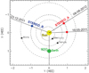 |
Fig. 1. Positions of SDO, Stereo_A, and Stereo_B in space during the observed events (the locations of spacecrafts and separation angles were obtained from STEREO web page at https://stereo-ssc.nascom.nasa.gov). |
In order to identify prominences on both SDO and STEREO datasets, we used the solar software (SSW) STEREO procedure wcs_convert_diff_rot, which takes heliographic coordinates of a set point on image from one spacecraft and applies a differential rotation model (another stereo procedure diff_rot.pro) to match the position of the point on another spacecraft image.
We used the path-draw functionality of The CRISP Spectral Explorer (CRISPEX; Vissers 2012) to trace falling material along visible trajectory and space-time diagrams on traced paths. From the space-time diagrams, we determined projected velocities and accelerations using the CRISPEX auxiliary program Timeslice ANAlysis Tool (TANAT; Vissers 2012).
3. Results
3.1. Event of May 16–18, 2011
The separation angle between SDO and Stereo_A was +93° on May 16, 2011; therefore, the eastern edge of the SDO image (the eastern limb) lies on −3° longitude on the Stereo_A image. The target prominence first appeared at the eastern limb on SDO images at 05:00 UT on May 16, 2011. At the same time, it was seen on disc near the western limb in Stereo_A. Figure 2 shows the evolution of the prominence from SDO and Stereo_A at 14:06 UT, May 16, 2011 and 00:06 UT, May 18, 2011. The left panels show composite images from SDO_AIA, and the right panels show 195 Å wavelength of Stereo_A-EUVI. White arrows show the points, which were identified with both spacecraft observations.
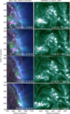 |
Fig. 2. Evolution of prominence from 14:06 UT, May 16, 2011 to 00:06 UT, May 18, 2011 in SDO/AIA and Stereo_A-EUVI. Left panels: composite images of 304 Å, 171 Å, and 193 Å wavelengths from SDO/AIA. Right panels: 195 Å wavelength of Stereo_A-EUVI. The white arrows in the top four frames indicate the specific points on images from both spacecraft. F1 points correspond to the footpoint of tornado-like structure. The brightening is marked with B1 and B2 points for identifying areas of interest. Approximate boundaries of prominence are shown by white dotted-curved lines in the lower four panels. |
A tornado-like structure started to rise up at 05:00 UT on May 16, 2011 (indicated by F1 in Fig. 2). To identify the area of interest more precisely, we also marked two small brightenings on images of both spacecrafts (indicated by B1 and B2). White dotted-curved lines in the lower panels of Fig. 2 show the mean edges of prominence tube.
Figure 3 shows the evolution of the prominence in 304 Å line of SDO/AIA at 14:06 UT (May 16, 2011)–06:36 UT (May 18, 2011). The massive fall of coronal rain from the prominence main body started at 22:00 UT (May 16, 2011) and continued until 02:00 UT (May 18, 2011). After almost 28 h of coronal rain, the prominence started to be destabilised and finally erupted as a CME on May 18, 2011.
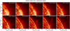 |
Fig. 3. Evolution of the prominence in 304 Å line of SDO_AIA from 14:06 UT, May 16, 2011 to 06:36 UT, May 18, 2011. |
Figure 4 shows a process of prominence rising in detail using a vertical space-time cut at a particular location indicated by a white dotted line in the upper left panel. The upper right panel shows the space-time diagram during the whole interval of the prominence evolution. it is seen that the whole rising process may be formally divided into two phases: a slow rise phase (from about 03:00 UT, May 17, 2011 to 04:00 UT, May 18, 2011) and a fast rise phase (from 04:00 UT, May 18, 2011). The fast rise phase corresponds to the final destabilisation and eruption of the prominence as a CME. The slow rise phase is probably connected to the slow loss of mass due to the rain (see Sect. 3.4).
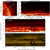 |
Fig. 4. Space-time diagram of prominence rise at a fixed cut in 304 Å line of SDO_AIA during 14:06 UT, May 16, 2011 and 11:30 UT, May 18, 2011 (top right panel). The location of the cut is shown by a white dashed line in the top left panel. Middle and the lower panels: zoomed-in image of a black box corresponding to the interval of 19:00 UT, May 16, 2011–02:00 UT, May 17, 2011 (that is before the start of slow rising) in 304 Å (middle panel) and 171 Å (lower panel) lines. |
In order to study the coronal rain, we traced the falling blobs along a visible trajectory from the SDO images and drew their paths using the path-draw functionality of CRISPEX (Vissers 2012). We identified 12 visible trajectories of falling plasma, which are shown as white dotted lines in the upper left panel of Fig. 5. Then, we constructed space-time diagrams for each trajectory. The lower panel of Fig. 5 shows the space-time diagram along the curved trajectory of number 6 indicated by the white arrow in the upper left panel. The white dashed-curves in this panel show well-defined trajectories of falling blobs. We fitted trajectories of all cuts with a polynomial and determined the average velocity of falling material as  = 23.5 km s−1. Acceleration of coronal rain blobs is estimated to be smaller than the free-fall in the solar atmosphere, as is typical for the rain.
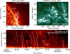 |
Fig. 5. Simultaneous images taken at 15:36 UT on May 17, 2011, from SDO_AIA and Stereo_A-EUVI. Top left panel: composite image of 12 visible trajectories of falling plasma with white dotted lines, from SDO_AIA. Top right frame: area of prominence tube with a red dashed line in 195 Å wavelength from Stereo_A-EUVI spacecraft. Bottom image: space-time diagram of falling plasma obtained from a typical cut along the traced path (the white arrows indicate the starting point and the position of the cut “6” trajectory in the top left panel). |
Prominence equilibrium is achieved by a balance between gravity and the Lorentz force of the prominence magnetic field. Coronal rain obviously took away a part of the prominence mass. Therefore, the reduction of the prominence mass may lead to the violation of the equilibrium and hence to the observed slow rise of the prominence. One can roughly estimate the mass loss of the prominence after 28 h of coronal rain. The total width of the 12 threads, where the coronal rain blobs were falling down, is around 12 SDO_AIA pixels, which corresponds to 0.864 × 109 cm (SDO_AIA pixel equal 720 km). Assuming the width as the tube diameter gives the total cross-section of coronal rain paths as 0.59 × 1018 cm2. Using the typical electron number density in prominence cores as ne = 1010 (Labrose et al. 2010), one can estimate prominence mean mass density as ρ = 1.67 × 10⁻¹⁴ g cm−3. Then, the mean speed of  km s−1 lead to the total mass flux of 2.32 × 10⁹ g s−1. Therefore, the estimated mass loss after 28 h coronal rain is ≈2.34 × 10¹⁵ g.
Simultaneous observations from SDO and STEREO allow us roughly estimate the prominence volume. Prominence length was estimated from STEREO data as 500 px, which with the STEREO pixel resolution of 1.6 arc sec gives 5.76 × 1010 cm (see red dashed area in the upper right panel of Fig. 5). The mean half-width of the prominence can be estimated as 30 px leading to 2.16 × 109 cm (Fig. 5 upper right panel). Assuming the half-width as the mean radius of cylindrical volume of the prominence, one can calculate the cross-section as 1.47 × 1019 cm2 and hence the prominence volume as 8.4 × 1029 cm3. Then, the prominence total mass is roughly estimated as 1.4 × 10¹⁶ g. The estimated mass loss suggests that around 17% of the prominence mass was taken away by the coronal rain before the final instability set-up at 04:00 UT, May 18, 2011. We note, however, that this estimation corresponds to the coronal rain only along one leg of the prominence, as we were not able to follow to dynamics of the another leg. If we suppose the similar mass flux along another leg, then the total mass loss can be estimated as 34% of the total mass.
When the prominence disappeared in the 304 Å line after the eruption, it was evidently detected in white light images of the Large Angle and Spectrometric Coronagraph (LASCO) instrument on the Solar and Heliospheric Observatory (SOHO) as a CME. Figure 6 shows the dynamics of the CME in the outer corona as observed from LASCO/C2, which covers a distance of 2.1–6 solar radii. According to the LASCO CME catalogue (Yashiro et al. 2004), the first appearance of the CME in the field of view C2 coronagraph is reported at 07:00:05 UT on May 18, 2011 with a speed of 141 km s−1. The CME appeared with an angular width of 36° in the northeast limb (see Fig. 6).
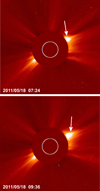 |
Fig. 6. CME eruption after the prominence instability as seen from LASCO_C2_SOHO. C2 displays an image in white light at a distance of 2.1–6 solar radii. The white arrows indicate the location of the CME. The two images show the time evolution of the CME at 07:24 UT (upper panel) and at 09:36 UT (lower panel) on May 18, 2011. |
3.2. Event of December 22–24, 2011
The separation angle between Stereo_B and SDO was −110° on December 22, 2011, hence the western limb of the SDO image corresponds to the +20° longitude on Stereo_ B image. The target prominence first appeared at the western limb on the SDO spacecraft at 11:00 UT on December 22, 2011. At the same time, it was seen on disc near the eastern limb in Stereo_ B. Figure 7 shows images from 20:06 UT (December 22, 2011) until 21:06 UT (December 23, 2011). The left panels show 195 Å wavelength of Stereo_ B/EUVI, and the right panels show composite images from SDO/AIA.
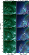 |
Fig. 7. Evolution of target prominence-filament from 20:06 UT, December 22, 2011 until 21:06 UT, December 23, 2011, in SDO and Stereo_B spectral lines. Right column: composite images of 304 Å, 171 Å, and 193 Å lines from SDO_AIA, Left column: the 195 Å line of Stereo_B-EUVI. White arrows marked with |


With the red dashed-curved line in the lower panels in Fig. 7, we marked approximate boundaries of prominence tube. We identified ten visible trajectories of falling plasma, which are shown as white dotted lines in the lower right panel of Fig. 7.
Figure 8 shows the evolution of the prominence in the 304 Å line of SDO/AIA from 20:06 UT (December 22, 2011) to 00:46 UT (December 24, 2011). Massive coronal rain started to flow down from the prominence main body at 20:00 UT (December 22, 2011) and continued until 21:45 UT (December 23, 2011), that is almost 26 h. The duration of coronal rain is similar to the previous case. After the coronal rain, the prominence became unstable on December 23, 2011 and finally erupted on December 24, 2011.
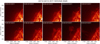 |
Fig. 8. Evolution of observed prominence with accompanied eruption in 304 Å wavelength of SDO/AIA from 20:06 UT, December 22, 2011 until 00:46 UT, December 24, 2011. |
As in the previous case, we fitted trajectories with a polynomial and determined the average velocity of coronal rain as  km s−1. The acceleration of coronal rain blobs is again smaller than the free-fall. The total width of the ten threads is around 10 pixels and consequently 7.2 × 108 cm (SDO/AIA pixel equal 720 km) with the total cross-section of coronal rain paths of 4.08 × 1017 cm2. This gives the total mass flux of 3.58 × 10¹⁰ g s−1 along one leg of the prominence leading to the mass loss of 3.35 × 10¹⁵ g in 26 h.
Prominence mean length and half-width are estimated from Stereo_ A/EUVI as ∼4 × 1010 cm (see red dashed area in lower left panel of Fig. 7) and ∼5.76 × 109 cm (Fig. 7 lower left panel), respectively, which lead to the prominence volume of ∼1.05 × 1030 cm3. Using the mean density of the prominence (see previous sub-section), one may estimate the prominence mass as 1.75 × 10¹⁶ g. Hence, due to the coronal rain, the prominence lost around 19% of its mass before it became unstable. Again, if we consider the symmetric mass flux along the both legs, then the mass loss rises up to 38%.
After the eruption, the prominence appeared in field of view C2 coronagraph at 00:36:05 UT, December 24, 2011 as a CME with a speed of 475 km s−1. Figure 9 shows the dynamics of the CME in the outer corona as observed from LASCO/C2. The CME appeared with an angular width of 61° in the northwest limb. Blue lines on the left panels of the time difference images show the position of the leading edge of the CME in the outer corona, while the red lines show an approximate outline to the leading edge that was created by using a segmentation technique (Olmedo et al. 2008), at the distance of 6.1 solar radii (images are taken from George Mason University Space Weather Lab project SEEDS: Solar Eruptive Events Detection System).
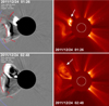 |
Fig. 9. CME eruption after the prominence instability as seen from LASCO_C2_SOHO. Left panels: running difference images, where the time difference is ∼36 min. The blue line indicates to the position of the leading edge, while the red line indicates an approximate outline to the leading edge. Right panels: images from LASCO_C2 coronagraph. The white arrows indicate the location of the CME. The two images show the time evolution of the CME during 01:26–02:48 UT on December 24, 2011. |
3.3. Event of August 07–08, 2012
The separation angle between SDO and Stereo_ A was −122° on August 07, 2012, therefore the eastern limb of the SDO images lie on −32° longitude on Stereo_ A images. The target prominence first appeared at the eastern limb on Stereo_ A at 09:06 UT on August 07, 2012. It was seen on disc near the western limb in SDO. Figure 10 shows the prominence from 09:06 UT, August 07, 2012 until 02:06 UT, August 08, 2012. The white dashed-curved line in the lower left panels of Fig. 10 shows approximate boundaries of the prominence tube. We identified ten visible trajectories of falling plasma, which are shown as white dotted lines in the lower right panel of Fig. 10.
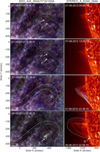 |
Fig. 10. Evolution of the Prominence from 09:06 UT, August 07, 2012 to 02:06 UT, August 08, 2012 in SDO_AIA and Stereo_A-EUVI. Left panels: composite images of 304 Å, 171 Å, and 193 Å wavelength from SDO/AIA. Right panels: 304 Å wavelength of Stereo_A-EUVI. The white arrows in the top four frames, marked with |


Figure 11 shows the evolution of the prominence in 304 Å line of Stereo_ A/EUVI from 09:06 UT (August 07, 2012) to 04:06 UT (August 08,2012). The massive fall of coronal rain started from the prominence main body at 09:06 UT (August 07, 2012) and continued until 04:06 UT (August 08, 2012), that is almost 18 h. The duration of coronal rain is shorter than in the previous cases. After the coronal rain, the prominence was destabilised on August 07, 2012 and finally erupted as a CME on August 08, 2012.
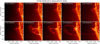 |
Fig. 11. Evolution of observed prominence in 304 Å wavelength of STEREO_EUVI between 09:06 UT, August 07, 2012 and 04:06 UT, August 08, 2012. |
The average velocity of coronal rain was estimated as  km s−1. The total width of the ten threads is around 1.15 × 109 cm, with the total cross section of coronal rain paths as 1.04 × 1018 cm2. This gives the total mass flux of 1.11 × 10¹⁰ g s−1 leading to the mass loss of 7.22 × 10¹⁵ g in 18 h. The prominence mean length and half-width are estimated from SDO/AIA as ∼1.01 × 1011 cm (see white dashed area in the lower left panel of Fig. 10) and ∼2.88 × 109 cm, respectively, which lead to the prominence mass as 4.39 × 10¹⁶ g. Then, the mass loss due to the coronal rain along one leg led to the reduction of the prominence mass with 17%.
Figure 12 shows the time difference images of the CME in the outer corona as observed from LASCO_C2. The CME appeared in the field of view C2 coronagraph at 05:48:07 UT, August 08, 2012 with a speed of 355 km s−1. In Fig. 12, the blue lines in the left panels of the time-difference images show the position of the leading edge of the CME in the outer corona, while the red lines show an approximate outline to the leading edge that was created by using a segmentation technique (images are taken from George Mason University Space Weather Lab project SEEDS: Solar Eruptive Events Detection System).
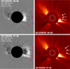 |
Fig. 12. CME eruption after the prominence instability as seen from LASCO_C2_SOHO. Left panels: running difference images, where the time difference is ∼35 min. The blue line indicates the position of the leading edge, while the red line indicates an approximate outline to the leading edge. The white arrows indicate the location of the CME. The two images show the time evolution of the CME during 06:48–07:36 UT on August 08, 2012. |
3.4. Possible mechanisms for the initial rise of prominence
As we already noted, a prominence is the result of equilibrium between magnetic and gravitational forces in the coronal low plasma-beta regime. Violation of the equilibrium resulting in the initial slow rise of prominence could be caused by two factors. Firstly, the thermal instability may result in the fall of coronal rain blobs, which reduces the prominence mass and hence leads to the slow rise of prominence. Secondly, the violation of equilibrium may be caused by a magnetic process (e.g., instability), which leads to the slow rise of prominence and consequently to the fall of prominence mass in form of blobs, as observed. In both cases, the coronal rain blobs are important ingredients in the process of slow rising. However, it is of vital importance to understand the triggering mechanism for initial rise of prominence body.
In order to study the process of initial rise, we considered the event of May 16–18, 2011 in detail. We zoomed out from the space-time diagram in Fig. 4 around the start of coronal rain, which was at 22:00 UT (May 16, 2011). Two lower panels show a zoomed-in image of the interval in two spectral lines. It is seen that the prominence was relatively stable until 00:30 UT (May 17, 2011), and then it started to rise slowly. Hence, the slow rise started after 2.5 h of the intensive coronal rain process (to follow the process of coronal rain from 22:00 UT (May 16, 2011)–00:30 UT (May 17, 2011); see accompanying movie). Obviously, when the prominence started to rise, the fall of plasma blobs from the prominence body is enhanced along magnetic field lines due to geometrical effects. However, the initial rise of prominence seems to be caused by coronal rain, which is presumably the result of thermal instability.
Vasantharaju et al. (2019) suggested that the slow rise phase may be connected with the ideal kink instability of flux rope. We examine this possibility for the event of May 16–18, 2011. In this case, the slow rise process continued from 03:00 UT, May 17, 2011 to 04:00 UT, May 18, 2011 that is about 25 h (Fig. 4). Growth time of ideal kink instability (Velli et al. 1990; Török et al. 2004; Zaqarashvili et al. 2010) is estimated as 10–100 transverse Alfvén time (the ratio of tube radius and Alfvén speed). The radius (or half-width) of the prominence flux tube is ∼20 Mm in our case, while the expected Alfvén speed in prominences is ∼10–20 km s−1. Then the growth time for ideal kink instability can be estimated as 0.3–0.5 h, which is much shorter than the slow rise time of the targeted prominence (25 h). Therefore, the kink instability is unlikely to be the reason for the slow rise of prominence body.
To check the dynamics of magnetic field configuration before and during the slow rise phase, we performed magnetic field extrapolation (potential-field source-surface – PFSS) using the standard PFSS package 1 available under SSW. Figure 13 shows that the magnetic field does not display any structural change during the slow rise phase, which indicates the absence of magnetic instability in this interval (the extrapolated field lines before and during the slow rise phase are shown on the upper and lower panels, respectively). This also indicates to the static configuration of photospheric magnetic field during the observed interval, which may rule out the role of photospheric changes in the slow rise process.
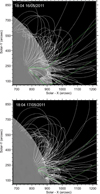 |
Fig. 13. Magnetic field extrapolation (potential-field source-surface PFSS) in prominence area before (at 18:04 UT, May 16, 2011 upper panel) and during (at 18:04 UT, May 17, 2011 lower panel) the slow rise process. White curves correspond to the close magnetic field lines, green (purple) lines show the open magnetic field lines with positive (negative) polarity. |
On the other hand, the fast rise phase probably corresponds to the magnetic instability, which can be processed either via the breakout model of coronal arcade (Antiochos et al. 1999) or torus instability of flux ropes (Török & Kliem 2007; Filippov 2013; Zuccarello et al. 2014). We cannot make a firm observational conclusion as to which of the two models work in our case. Figure 3 clearly shows the flux rope structure of the prominence in the fast rise phase, which may support the torus instability, but the breakout model cannot be completely ruled out. The prominence erupted as a CME into the outer corona as a result of the instability. Figure 14 shows the schematic picture of the whole process, which could be relevant to our case.
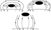 |
Fig. 14. Schematic dynamics of prominence evolution according to our model. Black ellipse represents the prominence and dashed-curved lines show the coronal rain blob trajectories. Initial configuration is shown by the upper left panel. Upper right panel displays the slow rise phase of the prominence triggered by the coronal rain. Final instability during fast rise phase and consecutive eruption of prominence as CME is shown on the lower panel. |
During the slow rise phase, the prominence body evolves slowly, which means that each consecutive configuration can be considered as a new equilibrium. Therefore, using the Kuperus-Raadu model of prominence equilibrium, one can write (Kuperus & Raadu 1974; Priest 1982):
 (1)
(1)
where B is the magnetic field strength, ρ is the plasma density, g is the surface gravitational acceleration, and h is the height from the surface. During the slow rise phase, the magnetic field does not change significantly (as is also shown by magnetic field extrapolation). Then, the slight increase of the prominence height must be balanced by slight decrease of the prominence density. Figure 15 shows the observed dynamics of prominence height and estimated decrease of density due to coronal rain during the whole interval. It is clearly seen that the height and density are in anti-phase: one increases and the other decreases. We also see that the slow rise of prominence is linear, indicating that the cause of the rising is not instability (see the exponential character in the fast rise phase). This rough estimation supports the suggestion that the slow rise of prominence is caused by the decrease of prominence mass due to coronal rain blobs.
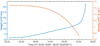 |
Fig. 15. Upward rise of the prominence along the cut on Fig. 4 (blue line) and estimated decrease of density due to coronal rain (red line) during the whole evolution of prominence in the event of May 16–18, 2011. |
4. Discussion
We analysed three solar prominences using simultaneous observations of SDO and Stereo spacecrafts during 2011–2012. The prominences were observed from different angles by different missions, which gave us the possibility to follow the dynamics of prominences in detail.
In all three cases, the massive coronal rain blobs started to flow from the prominence main bodies, then the prominences destabilised and erupted as CMEs. It is shown that after few hours of coronal rain, prominences started to rise, probably due to the mass loss. The rise of prominence consists of two phases: the initial slow rise phase and the consecutive fast rise phase.
We tracked falling coronal rain blobs along inclined trajectories (in total, 32 trajectories were detected in the three cases). From tracked trajectories, we extracted the space-time diagram to define acceleration and initial velocity of the falling plasma blobs. We fitted well-defined curved trajectories from space-time diagrams with polynomial fits and estimated initial velocity with a mean velocity around 65 km s−1, which correspond to the values reported in previous works (Schrijver 2001; De Groof et al. 2005; Antolin et al. 2010; Antolin & Verwichte 2011; Antolin & Rouppe van der Voort 2012).
Accelerations of coronal rain blobs were estimated as 20–136 m s−2, with a mean around 74 m s−2 from all tracked coronal rain blobs. The acceleration is smaller than the free-fall, as found in earlier works (Schrijver 2001; De Groof et al. 2004, 2005; Antolin et al. 2010; Antolin & Verwichte 2011; Antolin & Rouppe van der Voort 2012). The falling distances were more than 29 Mm for most of the blobs, and falling time was > 30 min, as reported in previous works (De Groof et al. 2004, 2005; Antolin et al. 2010; Antolin & Verwichte 2011; Antolin & Rouppe van der Voort 2012).
We estimated the prominence mass loss by coronal rain blobs before destabilisation at around 17–19%. However, in all three cases we only observed the coronal rain blobs along one leg of the prominences. Other legs were not seen by observations. If one assumes the symmetric mass flow happened along both legs, then the mass loss will increase to 34–38%. Therefore, one may conclude that the instability starts when prominences lose around 40% of their masses. If initial density in the considered prominences was as ρ = 1.67 × 10⁻¹⁴ g cm−3, then after the mass loss due to coronal rain the density may reach (considering unchanged volumes of prominence bodies) 1.11 × 10⁻¹⁴ g cm−3 (for the event of May 16–18, 2011), 1.02 × 10⁻¹⁴ g cm−3 (for the event of December 22–24, 2011), and 1.12 × 10⁻¹⁴ g cm−3 (for the event of August 07–08, 2012).
Understanding the triggering mechanism for the initial slow rise of prominence is of vital importance. The mechanism could be related to unstable magnetic field configuration such as the kink instability of twisted flux tubes. The growth time for the kink instability in prominence conditions can be estimated as < 1 h (see previous section). However, the slow rise phase lasts much longer in all three cases; it is around 25 h for the event of May 16–18 (2011), for example. Therefore, the kink instability can be ruled out as a triggering mechanism for the slow rise phase. On the other hand, reduction of density and mass in prominences due to the coronal rain obviously causes the reduction of gravity force, which eventually led to the excess of Lorentz force and hence upward motion of prominence bodies. We studied the detailed upward motion of the prominence using a space-time diagram for the event of May 16–18 (2011), which showed that the slow rise phase could be triggered by coronal rain. The slow rise of the prominence at some height may eventually lead to the torus instability (Török & Kliem 2007; Filippov 2013; Zuccarello et al. 2014) or reconnection with overlying coronal magnetic field according to the breakout model (Antiochos et al. 1999). The instabilities correspond to the fast rise phase, when prominences finally erupted as CMEs (see Fig. 14).
The time intervals between the start of coronal rain and final destabilisation of the prominence were estimated as 28 h for the event of May 16–18 (2011), 26 h for the event of December 22–24 (2011), and 18 h for the event of August 07–08 (2012). Therefore, if the coronal rain leads to the initial slow rise and the consequent final destabilisation of many prominences, one can predict CMEs 20–30 h before their actual eruptions. This will lead to considerable improvement of space weather predictions. This requires a detailed statistical study of the interconnection between coronal rain and CME initiations.
5. Conclusion
We studied the dynamics of three different prominences (May 16–18, 2011, December 22–24, 2011, and August 07–08, 2012) using simultaneous observational data from SDO_AIA and Stereo_SECCHI. The SDO and Stereo twin spacecrafts were observing the Sun from different angles; therefore, we were able to trace the evolution of the prominences in detail. In all three cases, the massive coronal rain started to fall down towards the photosphere, which was followed by the destabilisation of prominences after 20–30 h and later by CMEs. The upward rise of prominence consisted of two phases: an initial slow rise phase and a consecutive fast rise phase. We suggest that the slow rise phase was triggered by the violation of equilibrium between gravity and Lorentz forces as the result of the mass loss due to coronal rain. On the other hand, the fast rise phase was probably connected with magnetic instability or reconnection, which led to the final destabilisation of the prominences. Estimations of mass flux along one leg of the prominences (another legs were not seen by observations) led to 20% of the mass loss before the final destabilisation. Assuming the symmetric mass flux along the both legs, one can conclude that the prominences became unstable after the loss of 40% of their masses. If future analysis shows the similar behaviour for many prominences, then the coronal rain may be used to predict the prominence instability and hence CMEs. This will help to improve the space weather predictions.
Acknowledgments
Work was supported by the Shota Rustaveli National Science Foundation (SRNSF) grant DI-2016-52, The work of TVZ and AH was funded by the Austrian Science Fund (FWF, projects P30695-N27 and I 3955-N27). PG acknowledges the support of the project VEGA 2/0048/20, We thank the anonymous referee for useful comments, which led to improving the paper significantly.
References
- Antiochos, S. K., MacNeice, P. J., Spicer, D. S., & Klimchuk, J. A. 1999, ApJ, 512, 985 [Google Scholar]
- Antolin, P., & Verwichte, E. 2011, ApJ, 736, 121 [NASA ADS] [CrossRef] [Google Scholar]
- Antolin, P., & Rouppe van der Voort, L. 2012, ApJ, 745, 152 [Google Scholar]
- Antolin, P., Shibata, K., & Vissers, G. 2010, ApJ, 716, 154 [NASA ADS] [CrossRef] [Google Scholar]
- Arregui, I., Oliver, R., & Ballester, J. L. 2012, Liv. Rev. Sol. Phys., 9, 2 [Google Scholar]
- Chae, J., Denker, C., Spirock, T. J., et al. 2000, Sol. Phys., 195, 333 [NASA ADS] [CrossRef] [Google Scholar]
- De Groof, A., Berghmans, D., van Driel-Gesztelyi, L., & Poedts, S. 2004, A&A, 415, 1141 [NASA ADS] [CrossRef] [EDP Sciences] [Google Scholar]
- De Groof, A., Müller, D. A. N., Berghmans, D., & Poedts, S. 2005, A&A, 443, 319 [NASA ADS] [CrossRef] [EDP Sciences] [Google Scholar]
- Field, G. B. 1965, ApJ, 142, 531 [Google Scholar]
- Filippov, B. 2013, ApJ, 773, 10 [NASA ADS] [CrossRef] [Google Scholar]
- Gopalswamy, N., Shimojo, M., Lu, W., et al. 2003, ApJ, 586, 562 [NASA ADS] [CrossRef] [Google Scholar]
- Kuperus, M., & Raadu, M. A. 1974, A&A, 31, 189 [NASA ADS] [Google Scholar]
- Labrose, N., Heinzel, P., Vial, J. C., et al. 2010, Space Sci. Rev., 151, 243 [CrossRef] [Google Scholar]
- Lemen, J. R., Title, A. M., Akin, D. J., et al. 2012, Sol. Phys., 275, 17 [Google Scholar]
- Liu, W., Berger, T. E., & Low, B. C. 2012, ApJ, 745, L21 [Google Scholar]
- Müller, D. A. N., Hansteen, V. H., & Peter, H. 2003, A&A, 411, 605 [NASA ADS] [CrossRef] [EDP Sciences] [Google Scholar]
- Müller, D. A. N., Peter, H., & Hansteen, V. H. 2004, A&A, 422, 289 [CrossRef] [EDP Sciences] [Google Scholar]
- Müller, D. A. N., De Groof, A., Hansteen, V. H., & Peter, H. 2005, A&A, 436, 1067 [NASA ADS] [CrossRef] [EDP Sciences] [Google Scholar]
- Ning, Z., Cao, W., & Goode, P. R. 2009, ApJ, 707, 1124 [NASA ADS] [CrossRef] [Google Scholar]
- Olmedo, O., Zhang, J., Wechsler, H., Poland, A., & Borne, K. 2008, Sol. Phys., 248, 485 [NASA ADS] [CrossRef] [Google Scholar]
- Panesar, N. K. 2014, PhD Thesis (Germany: Georg-August-Universität Göttingen, Institut für Astrophysik) [Google Scholar]
- Parker, E. N. 1953, ApJ, 117, 431 [Google Scholar]
- Pesnell, W. D., Thompson, B. J., & Chamberlin, P. C. 2012, Sol. Phys., 275, 3 [Google Scholar]
- Priest, E. R. 1982, Solar Magnetohydrodynamics (Dordrecht: D. Reidel Publ. Co.) [CrossRef] [Google Scholar]
- Priest, E. R., & Forbes, T. G. 2002, A&ARv, 10, 313 [Google Scholar]
- Schmieder, B., Van Driel-Gesztelyi, L., & Aulanier, G. 2002, Adv. Space Res., 29, 1451 [NASA ADS] [CrossRef] [Google Scholar]
- Schrijver, C. J. 2001, Sol. Phys., 198, 325 [Google Scholar]
- Shen, Y., Liu, Y., Liu, Y. D., et al. 2015, ApJ, 814, L17 [Google Scholar]
- Su, Y., Wang, T., Veronig, A., et al. 2012, ApJ, 756, L41 [NASA ADS] [CrossRef] [Google Scholar]
- Török, T., & Kliem, B. 2007, Astron. Nachr., 328, 743 [CrossRef] [Google Scholar]
- Török, T., Kliem, B., & Titov, V. S. 2004, A&A, 413, L27 [NASA ADS] [CrossRef] [EDP Sciences] [Google Scholar]
- Vasantharaju, N., Vemareddy, P., Ravindra, B., & Doddamani, V. H. 2019, ApJ, 885, 89 [NASA ADS] [CrossRef] [Google Scholar]
- Vashalomidze, Z., Kukhianidze, V., Zaqarashvili, T. V., et al. 2015, A&A, 577, A136 [NASA ADS] [CrossRef] [EDP Sciences] [Google Scholar]
- Velli, M., Einaudi, G., & Hood, A. W. 1990, ApJ, 350, 428 [NASA ADS] [CrossRef] [Google Scholar]
- Vissers, G. 2012, ApJ, 750, 22 [NASA ADS] [CrossRef] [Google Scholar]
- Williams, D. R., Török, T., Démoilin, P., van Driel-Gesztelyi, L., & Kliem, B. 2005, ApJ, 628, L163 [NASA ADS] [CrossRef] [Google Scholar]
- Yashiro, S., Gopalswamy, N., Michalek, G., et al. 2004, JGRA (Space Phys.), 109, A07105 [NASA ADS] [Google Scholar]
- Zaqarashvili, T. V., Diaz, A. J., Oliver, R., & Ballester, J. L. 2010, A&A, 516, A84 [NASA ADS] [CrossRef] [EDP Sciences] [Google Scholar]
- Zhang, Q. M., Li, T., Zheng, R. S., et al. 2017a, ApJ, 842, 27 [CrossRef] [Google Scholar]
- Zhang, Q. M., Li, D., & Ning, Z. J. 2017b, ApJ, 851, 47 [NASA ADS] [CrossRef] [Google Scholar]
- Zirker, J. B., Engvold, O., & Martin, S. F. 1998, Nature, 396, 440 [Google Scholar]
- Zuccarello, F. P., Seaton, D. B., Filippov, B., Mierla, M., et al. 2014, ApJ, 795, 175 [NASA ADS] [CrossRef] [Google Scholar]
All Figures
|
Fig. 1. Positions of SDO, Stereo_A, and Stereo_B in space during the observed events (the locations of spacecrafts and separation angles were obtained from STEREO web page at https://stereo-ssc.nascom.nasa.gov). |
| In the text | |
|
Fig. 2. Evolution of prominence from 14:06 UT, May 16, 2011 to 00:06 UT, May 18, 2011 in SDO/AIA and Stereo_A-EUVI. Left panels: composite images of 304 Å, 171 Å, and 193 Å wavelengths from SDO/AIA. Right panels: 195 Å wavelength of Stereo_A-EUVI. The white arrows in the top four frames indicate the specific points on images from both spacecraft. F1 points correspond to the footpoint of tornado-like structure. The brightening is marked with B1 and B2 points for identifying areas of interest. Approximate boundaries of prominence are shown by white dotted-curved lines in the lower four panels. |
| In the text | |
|
Fig. 3. Evolution of the prominence in 304 Å line of SDO_AIA from 14:06 UT, May 16, 2011 to 06:36 UT, May 18, 2011. |
| In the text | |
|
Fig. 4. Space-time diagram of prominence rise at a fixed cut in 304 Å line of SDO_AIA during 14:06 UT, May 16, 2011 and 11:30 UT, May 18, 2011 (top right panel). The location of the cut is shown by a white dashed line in the top left panel. Middle and the lower panels: zoomed-in image of a black box corresponding to the interval of 19:00 UT, May 16, 2011–02:00 UT, May 17, 2011 (that is before the start of slow rising) in 304 Å (middle panel) and 171 Å (lower panel) lines. |
| In the text | |
|
Fig. 5. Simultaneous images taken at 15:36 UT on May 17, 2011, from SDO_AIA and Stereo_A-EUVI. Top left panel: composite image of 12 visible trajectories of falling plasma with white dotted lines, from SDO_AIA. Top right frame: area of prominence tube with a red dashed line in 195 Å wavelength from Stereo_A-EUVI spacecraft. Bottom image: space-time diagram of falling plasma obtained from a typical cut along the traced path (the white arrows indicate the starting point and the position of the cut “6” trajectory in the top left panel). |
| In the text | |
|
Fig. 6. CME eruption after the prominence instability as seen from LASCO_C2_SOHO. C2 displays an image in white light at a distance of 2.1–6 solar radii. The white arrows indicate the location of the CME. The two images show the time evolution of the CME at 07:24 UT (upper panel) and at 09:36 UT (lower panel) on May 18, 2011. |
| In the text | |
|
Fig. 7. Evolution of target prominence-filament from 20:06 UT, December 22, 2011 until 21:06 UT, December 23, 2011, in SDO and Stereo_B spectral lines. Right column: composite images of 304 Å, 171 Å, and 193 Å lines from SDO_AIA, Left column: the 195 Å line of Stereo_B-EUVI. White arrows marked with |
| In the text | |
|
Fig. 8. Evolution of observed prominence with accompanied eruption in 304 Å wavelength of SDO/AIA from 20:06 UT, December 22, 2011 until 00:46 UT, December 24, 2011. |
| In the text | |
|
Fig. 9. CME eruption after the prominence instability as seen from LASCO_C2_SOHO. Left panels: running difference images, where the time difference is ∼36 min. The blue line indicates to the position of the leading edge, while the red line indicates an approximate outline to the leading edge. Right panels: images from LASCO_C2 coronagraph. The white arrows indicate the location of the CME. The two images show the time evolution of the CME during 01:26–02:48 UT on December 24, 2011. |
| In the text | |
|
Fig. 10. Evolution of the Prominence from 09:06 UT, August 07, 2012 to 02:06 UT, August 08, 2012 in SDO_AIA and Stereo_A-EUVI. Left panels: composite images of 304 Å, 171 Å, and 193 Å wavelength from SDO/AIA. Right panels: 304 Å wavelength of Stereo_A-EUVI. The white arrows in the top four frames, marked with |
| In the text | |
|
Fig. 11. Evolution of observed prominence in 304 Å wavelength of STEREO_EUVI between 09:06 UT, August 07, 2012 and 04:06 UT, August 08, 2012. |
| In the text | |
|
Fig. 12. CME eruption after the prominence instability as seen from LASCO_C2_SOHO. Left panels: running difference images, where the time difference is ∼35 min. The blue line indicates the position of the leading edge, while the red line indicates an approximate outline to the leading edge. The white arrows indicate the location of the CME. The two images show the time evolution of the CME during 06:48–07:36 UT on August 08, 2012. |
| In the text | |
|
Fig. 13. Magnetic field extrapolation (potential-field source-surface PFSS) in prominence area before (at 18:04 UT, May 16, 2011 upper panel) and during (at 18:04 UT, May 17, 2011 lower panel) the slow rise process. White curves correspond to the close magnetic field lines, green (purple) lines show the open magnetic field lines with positive (negative) polarity. |
| In the text | |
|
Fig. 14. Schematic dynamics of prominence evolution according to our model. Black ellipse represents the prominence and dashed-curved lines show the coronal rain blob trajectories. Initial configuration is shown by the upper left panel. Upper right panel displays the slow rise phase of the prominence triggered by the coronal rain. Final instability during fast rise phase and consecutive eruption of prominence as CME is shown on the lower panel. |
| In the text | |
|
Fig. 15. Upward rise of the prominence along the cut on Fig. 4 (blue line) and estimated decrease of density due to coronal rain (red line) during the whole evolution of prominence in the event of May 16–18, 2011. |
| In the text | |
Current usage metrics show cumulative count of Article Views (full-text article views including HTML views, PDF and ePub downloads, according to the available data) and Abstracts Views on Vision4Press platform.
Data correspond to usage on the plateform after 2015. The current usage metrics is available 48-96 hours after online publication and is updated daily on week days.
Initial download of the metrics may take a while.