| Issue |
A&A
Volume 657, January 2022
|
|
|---|---|---|
| Article Number | A56 | |
| Number of page(s) | 41 | |
| Section | Extragalactic astronomy | |
| DOI | https://doi.org/10.1051/0004-6361/202141488 | |
| Published online | 07 January 2022 | |
The MeerKAT Galaxy Cluster Legacy Survey
I. Survey Overview and Highlights⋆
1
Astrophysics Research Centre, University of KwaZulu-Natal, Durban 4041, South Africa
e-mail: This email address is being protected from spambots. You need JavaScript enabled to view it.
2
Centre for Radio Astronomy Techniques and Technologies, Department of Physics and Electronics, Rhodes University, PO Box 94 Makhanda 6140, South Africa
3
South African Radio Astronomy Observatory, 2 Fir Street, Observatory 7925, South Africa
4
National Radio Astronomy Observatory, Charlottesville, VA 22903, USA
5
Minnesota Institute for Astrophysics, University of Minnesota, 116 Church St SE, Minneapolis, MN 55455, USA
6
Wits Centre for Astrophysics, School of Physics, University of the Witwatersrand, 1 Jan Smuts Avenue, Johannesburg 2050, South Africa
7
Department of Physics, University of Pretoria, Hatfield 0028, South Africa
8
INAF – Osservatorio Astronomico di Cagliari, Via della Scienza 5, 09047 Selargius, CA, Italy
9
Hartebeesthoek Radio Astronomy Observatory, SARAO, Krugersdorp 1740, South Africa
10
York University, Toronto, ON, Canada
11
Hamburger Sternwarte, Universität Hamburg, Gojenbergsweg 112, 21029 Hamburg, Germany
12
Department of Astronomy, University of Cape Town, Rondebosch 7700, South Africa
13
Centre for Space Research, North-West University, Potchefstroom 2520, South Africa
14
Department of Physics and Astronomy, Faculty of Physical Sciences, University of Nigeria, Carver Building, 1 University Road, Nsukka, Nigeria
15
Naval Research Laboratory, Washington, DC 20375, USA
16
INAF – Istituto di Radioastronomia, Via Gobetti 101, 40129 Bologna, Italy
17
Argelander-Institut für Astronomie, Universität Bonn, Auf dem Hügel 71, 53121 Bonn, Germany
18
School of Mathematics, Statistics, and Computer Science, University of KwaZulu-Natal, Westville 3696, South Africa
19
Department of Physics and Astronomy, University of the Western Cape, Bellville 7535, South Africa
20
Dipartimento di Fisica, Universitá Sapienza, P.le Aldo Moro 2, 00185 Roma, Italy
21
African Institute for Mathematical Sciences, 6-8 Melrose Road, Muizenberg 7945, South Africa
22
Inter-University Institute for Data Intensive Astronomy, University of Cape Town, Rondebosch 7700, South Africa
23
Tellumat (Pty) Ltd., 64-74 White Road, Retreat 7945, South Africa
24
EMSS Antennas, 18 Techno Avenue, Technopark, Stellenbosch 7600, South Africa
25
SKA Observatory, Jodrell Bank, Lower Withington, Macclesfield, Cheshire SK11 9FT, UK
26
Department of Electrical and Electronic Engineering, Stellenbosch University, Stellenbosch 7600, South Africa
27
Oxford Astrophysics, Denys Wilkinson Building, Keble Road, Oxford OX1 3RH, UK
28
, 12 Blaauwklippen Rd, Kirstenhof 7945, South Africa
29
Presidential Infrastructure Coordinating Commission, 77 Meintjies Street, Sunnyside 0001, South Africa
30
Indian Institute of Astrophysics, II Block, Koramangala, Bengaluru 560 034, India
31
GEPI, Observatoire de Paris, CNRS, PSL Research University, Université Paris Diderot, 92190 Meudon, France
32
Peralex (Pty) Ltd., 5 Dreyersdal Rd, Bergvliet 7945, South Africa
Received:
7
June
2021
Accepted:
25
October
2021
Abstract
MeerKAT’s large number (64) of 13.5 m diameter antennas, spanning 8 km with a densely packed 1 km core, create a powerful instrument for wide-area surveys, with high sensitivity over a wide range of angular scales. The MeerKAT Galaxy Cluster Legacy Survey (MGCLS) is a programme of long-track MeerKAT L-band (900−1670 MHz) observations of 115 galaxy clusters, observed for ∼6−10 h each in full polarisation. The first legacy product data release (DR1), made available with this paper, includes the MeerKAT visibilities, basic image cubes at ∼8″ resolution, and enhanced spectral and polarisation image cubes at ∼8″ and 15″ resolutions. Typical sensitivities for the full-resolution MGCLS image products range from ∼3−5 μJy beam−1. The basic cubes are full-field and span 2° × 2°. The enhanced products consist of the inner 1.2° × 1.2° field of view, corrected for the primary beam. The survey is fully sensitive to structures up to ∼10′ scales, and the wide bandwidth allows spectral and Faraday rotation mapping. Relatively narrow frequency channels (209 kHz) are also used to provide H I mapping in windows of 0 < z < 0.09 and 0.19 < z < 0.48. In this paper, we provide an overview of the survey and the DR1 products, including caveats for usage. We present some initial results from the survey, both for their intrinsic scientific value and to highlight the capabilities for further exploration with these data. These include a primary-beam-corrected compact source catalogue of ∼626 000 sources for the full survey and an optical and infrared cross-matched catalogue for compact sources in the primary-beam-corrected areas of Abell 209 and Abell S295. We examine dust unbiased star-formation rates as a function of cluster-centric radius in Abell 209, extending out to 3.5 R 200. We find no dependence of the star-formation rate on distance from the cluster centre, and we observe a small excess of the radio-to-100 μm flux ratio towards the centre of Abell 209 that may reflect a ram pressure enhancement in the denser environment. We detect diffuse cluster radio emission in 62 of the surveyed systems and present a catalogue of the 99 diffuse cluster emission structures, of which 56 are new. These include mini-halos, halos, relics, and other diffuse structures for which no suitable characterisation currently exists. We highlight some of the radio galaxies that challenge current paradigms, such as trident-shaped structures, jets that remain well collimated far beyond their bending radius, and filamentary features linked to radio galaxies that likely illuminate magnetic flux tubes in the intracluster medium. We also present early results from the H I analysis of four clusters, which show a wide variety of H I mass distributions that reflect both sensitivity and intrinsic cluster effects, and the serendipitous discovery of a group in the foreground of Abell 3365.
Key words: surveys / galaxies: clusters: general / radio continuum: general / catalogs / radio lines: general / galaxies: general
Data are available at https://doi.org/10.48479/7epd-w356.
© ESO 2022
1. Introduction
Galaxy clusters are the largest gravitationally bound structures in the Universe and, as such, are powerful tools for a variety of research areas in both astrophysics and cosmology. Their composition is dominated by dark matter, with ∼13% of their mass coming from the ionised plasma of the intracluster medium (ICM) and only ∼2% from the stars of their constituent galaxies and cold gas. Some of these galaxies radiate at radio frequencies, either through star-formation processes or from nuclear activity in the galaxy’s core (Condon 1992; Simpson et al. 2006; Luchsinger et al. 2015; Mancuso et al. 2017). Some radio galaxies with active galactic nuclei (AGN) exhibit large-scale radio jets or lobes (Fanaroff & Riley 1974), which can be disrupted by interaction with the ICM through merger-related or other processes (see e.g. Gunn & Gott 1972; Miley et al. 1972; Cowie & McKee 1975; Blanton et al. 2003).
Radio observations of clusters have also revealed steep-spectrum, diffuse radio emission (see reviews by Feretti et al. 2012; van Weeren et al. 2019), which can be used to study the distributed populations of cosmic ray particles and magnetic fields in the ICM, outside of individual radio or star-forming galaxies. These diffuse structures are closely linked to cluster mergers (Cassano et al. 2010; van Weeren et al. 2011a) and as such can also be used to study shock physics, merger-related turbulence, and other particle re-acceleration processes within the ICM (see reviews by Brunetti & Jones 2014; van Weeren et al. 2019, and references therein). Cluster observations carried out by wide-field instruments also contain many field sources, both along the cluster line of sight and in the surrounding area. These provide important information on the clusters themselves (e.g. by using background sources as Faraday rotation probes) and on radio galaxy physics outside of the dense cluster environments. Wide-field imaging enables both statistical studies, such as environment-sensitive properties of galaxy populations, and serendipitous studies of individual field sources (e.g. Brüggen et al. 2021).
MeerKAT1 is a 64-dish radio interferometer that can observe the sky below a declination (Dec) of +45° (with an elevation limit of 15°), operating in the UHF (580−1015 MHz), L (900−1670 MHz), and S bands (1.75−3.5 GHz). Its specifications are described in detail in Jonas & MeerKAT Team (2016) and Camilo et al. (2018). MeerKAT’s L-band system, with a primary beam full width at half maximum (FWHM) of 1.2° at 1.28 GHz, was the first to be commissioned, and in 2018 MeerKAT began a programme of long-track observations of galaxy clusters. This programme became the MeerKAT Galaxy Cluster Legacy Survey (MGCLS), using ∼1000 h in the L band to observe 115 galaxy clusters in full polarisation between −80° and 0° Dec, spread out over the full range of right ascension (RA).
In addition to continuum and polarimetric studies, the deep, broadband, wide-field, sub-10″ resolution MGCLS observations provide a rich resource for studying neutral hydrogen in galaxies. Studies of H I morphologies in dense cluster environments and in the field, distributions of H I masses in different types of clusters, and the cosmic evolution of cluster H I out to redshifts of z = 0.48 are all enabled with these data, with a velocity resolution of ∼44 km s−1 at z = 0.
Here we present an overview of the MGCLS and the various legacy products being made available to the astronomical community. These data are a rich resource for many scientific studies, both cluster-specific studies and those involving field sources. We provide some initial science findings in the areas of cluster diffuse emission, radio galaxy physics, star-forming systems, and neutral hydrogen mapping. In addition to their intrinsic value, these examples also demonstrate the potential of the legacy products for a wide range of astrophysical investigations.
The paper is organised as follows. In Sect. 2 we describe the target sample, with the observations and initial data processing described in Sect. 3. A discussion of the legacy data products, including caveats for use and some primary use cases, is provided in Sect. 4. Source catalogues are presented in Sect. 5. The next four sections present highlights of various science investigations that have been or can be carried out using the legacy products and visibilities: Sect. 6 focuses on cluster diffuse emission; Sect. 7 highlights some interesting individual radio sources; Sect. 8 presents results based on star-forming galaxies; and Sect. 9 highlights some H I science capabilities. A summary and concluding remarks are presented in Sect. 10. In this paper we assume a flat Λ cold dark matter cosmology with H0 = 70 km s−1 Mpc−1, Ωm = 0.3, and ΩΛ = 0.7. We define the radio spectral index, α, such that Sν ∝ να, where Sν is the flux density at frequency ν. In this paper R200 denotes the radius within which the average density is 200 times the critical density of the Universe. Unless otherwise noted, we give all synthesised beams in terms of FWHM values, and redshifts are taken from the NASA/IPAC right ascension (NED)2 (Helou et al. 1991) or VizieR (Ochsenbein et al. 2000).
2. Cluster sample
The MGCLS sample consists of 115 galaxy clusters spanning a Dec range of −85 to 0°. The targeted clusters form a heterogeneous sample, with no mass or redshift selection criteria applied, and consist of two groups: ‘radio-selected’ and ‘X-ray-selected’. The full list of MGCLS clusters is given in Table 1 where the listed RA and Dec are that of the MeerKAT pointing. The median redshift of the sample is 0.14, with only four clusters at z > 0.4.
Observed cluster sample.
2.1. Radio-selected sub-sample
The radio-selected sub-sample consists of 41 southern targets that have been previously searched for diffuse cluster radio emission by other studies. Targets were selected from published radio studies or reviews, namely Giovannini et al. (1999), Feretti et al. (2012), Lindner et al. (2014), Kale et al. (2015, 2017), Shakouri et al. (2016), Bonafede et al. (2017), George et al. (2017), Giacintucci et al. (2017), Parekh et al. (2017), and Golovich et al. (2019), and include both systems with and without previous diffuse emission detections. These previous radio studies were restricted to high-mass systems, M500 ≳ 6 × 10¹⁴ M⊙, derived from X-ray or Sunyaev-Zel’dovich effect (Sunyaev & Zeldovich 1972) data. Thus, the radio-selected sub-sample contains only high mass clusters. It covers a redshift range of 0.018 < z < 0.87, with median z = 0.22.
Targeting systems of this nature ensured a high scientific return in terms of diffuse emission studies. However, due to the selection, this sub-sample is strongly biased towards clusters with radio halos and relics. The radio-selected clusters are listed in the first panel of Table 1, using their common names. Where available, an alternate name is provided in the final column of the table. In cases where multiple alternate names exist, the Meta-Catalogue of X-ray-detected Clusters (MCXC; Piffaretti et al. 2011) designation, if available, is given.
2.2. X-ray-selected sub-sample
The X-ray-selected sub-sample, making up 64% of the MGCLS, was selected from the MCXC catalogue, in order to create a sample with no direct prior biases towards or against cluster radio properties. From the list of clusters in the MCXC catalogue that were south of −39°, we selected MGCLS targets as needed to fill gaps in MeerKAT’s observing schedule.
The X-ray-selected clusters, which cover a redshift range of 0.011 < z < 0.640 with a median of z = 0.13, are listed in the second panel of Table 1 using their MCXC catalogue designations. Where relevant, common alternate names are also listed. The X-ray-selected sample covers a luminosity range of LX ∼ (0.1 − 30)×1044 erg s−1, with ∼60% of clusters in the range 1044 − 1045 erg s−1.
3. Observations and data reduction
3.1. Observations
The MGCLS observations were carried out between June 24, 2018, and June 16, 2019, using the full MeerKAT array, with a minimum of 59 antennas per observation. The MGCLS clusters were observed using MeerKAT’s L-band receiver (with nominal radio frequency band of 900−1670 MHz) in the 4k correlator mode (4096 channels across the digitised band of 856−1712 MHz) with 8 s integrations.
Data consists of all combinations of the two orthogonal linearly polarised feeds. Each dataset contains observations of the flux density, delay, and bandpass calibrators PKS B1934−638 and/or PMN J0408−6545. These were observed for 10 min every hour with the remaining time cycling between the target cluster (10 min) and a nearby astrometric and phase calibrator (1 min). These observations spanned 8−12 h, cycling between the target cluster and the various calibrator sources, and typically consisted of ∼5.5−9.5 h on source integration, sometimes divided into multiple sessions. These were scheduled as ‘fillers’ during observing schedule gaps.
3.2. Initial processing
All datasets were calibrated and imaged with a simple procedure, described in Mauch et al. (2020), which also verified the data quality. All calibration and imaging used the OBIT package3 (Cotton 2008).
3.2.1. Calibration and editing
Various processes as described in Mauch et al. (2020) were used to identify data affected by interference and/or equipment failures, which were then edited out, typically resulting in ∼50% of the frequency and/or time samples being removed. The remaining data were calibrated in group delay, bandpass, and amplitude and phase. The reference antenna was picked on the basis of the best signal-to-noise ratio (S/N) in the bandpass solutions. Our flux density scale is based on the spectrum of PKS B1934−638 (Reynolds 1994):
 (1)
(1)
where S is the flux density in Jy and ν is the frequency in MHz. The uncertainty in the flux-density scale is estimated to be ∼5%.
Small errors in both time and frequency tagging were discovered after the observations had started and were subsequently corrected. These errors have a small effect on the images, and are more fully described in Sect. 4.4.4. The majority of images were made after the errors were fixed.
3.2.2. Stokes-I imaging
We created the maps using the OBIT wide-band, wide-field imager MFImage. MFImage uses facets to correct for the curvature of the sky, and multiple frequency bins, which are imaged independently and deconvolved jointly, to allow for the antenna gains and a sky brightness distribution that vary with frequency. A frequency-dependent taper was used to obtain a resolution that remained approximately constant over our ∼2:1 range in frequency. MFImage is described in more detail in Cotton et al. (2018).
The sky within a radius of 0.8° to 1° of the pointing centre was fully imaged, with outlying facets added to cover sources from the Sydney University Molonglo Sky Survey (SUMSS; Bock et al. 1999) 843 MHz catalogue (Mauch et al. 2003) brighter than 5 mJy within 1.5°. Two iterations of phase-only self-calibration, with a 30 s solution interval, were used. Amplitude and phase self-calibration were added if the image contained a pixel with a brightness in excess of 0.3 Jy beam−1. For Stokes-I imaging we used a maximum of 30 000 components, a loop gain of 0.1, and fields were typically CLEANed to a depth of ∼50 μJy beam−1. No direction-dependent corrections were applied; such corrections may be useful for followup studies of individual fields, but do not affect the science results presented here.
Robust weighting (−1.5 in AIPS/OBIT usage) was used to down-weight the very densely sampled inner portion of the uv-plane. The resulting FWHM resolution was in the range 7.5−8.0″. We made images consisting of 14 frequency bins, each with a 5% fractional (Δν/ν) bandpass. When the imaging was complete, a spectrum was fitted in each pixel of the resulting cube. Off-source noise levels (rms) in images that were not dynamic range limited ranged over ∼3−5 μJy beam−1. This is close to the expected thermal noise, with rms confusion expected to be of the order of 1 μJy beam−1 (Mauch et al. 2020). The local rms noise varies over the field of view due to contributions from (multiple) strong sources and is a strong function of the target pointing. Primary beam corrections were only applied to the ‘enhanced products’ (see Sect. 4.2).
3.2.3. Reprocessing with polarimetry
Changes from the standard procedure described in Sect. 3.2.1 were needed for polarisation calibration. The MGCLS observations did not contain observations of a polarised calibrator to calibrate the polarisation response of the array. However, each MeerKAT observing session is begun with a calibration using noise signals injected into each antenna that can be used to calibrate the bulk of the phase and delay difference between the two recorded orthogonal linear polarisations. The remainder of the signal path is stable enough that, after this initial calibration, appropriate polarisation calibration is possible using calibration parameters derived from other, properly polarisation-calibrated, data. This procedure is discussed in detail in Plavin et al. (2020); however, we outline the basic steps here for clarity.
Prior to any calibration derived from the data, the initial calibration of the ‘X’ and ‘Y’ linear feeds from the injected noise signals was performed; this removes most of the phase and delay difference between the X and Y systems. The remainder is sufficiently stable that a ‘standard’ calibration using the same reference antenna corrects it. In the parallel hand calibration the two bandpass calibrators, PKS B1934−638 and PMN J0408−6545, are sufficiently weakly polarised that they can be considered unpolarised. After bandpass calibration subsequent gain calibration solved only for Stokes-I terms to avoid disturbing the relative X/Y gain ratio.
Following the parallel-hand calibration, our polarisation calibration procedure was as follows. We required the selected calibration reference antenna to have a set of averaged polarisation calibrations derived from other MeerKAT datasets that had adequate polarisation calibration (including a polarised calibrator). This ‘standard’ set of calibration tables was used to complete the X−Y phase calibration and to correct for on-axis instrumental polarisation via the feed ellipticity and orientation4. Since the antennas are equipped with linear feeds, the fundamental reference for the polarisation angle is the nominal orientation of the feeds.
The standard polarisation calibration source 3C286 was used to verify and make final corrections to the polarisation calibration. This source has a polarisation angle of −33° and a rotation measure (RM) equal to zero (Perley & Butler 2013). A correction of several degrees in polarisation angle and about 1 rad m−2 in RM is needed to reproduce the assumed polarisation. These corrections are stable over several years and have been applied to all polarisation corrected data.
A selected subset of the clusters were re-calibrated and imaged in MFImage to produce Stokes I, Q, U, and V images; these clusters are indicated in the ‘Poln’ column in Table 1. Due to the lack of internal polarisation calibration, the Stokes V images are not sufficient to detect weakly circular polarised sources, but can work as an overall check of the quality of the calibration. Strongly circularly or linearly polarised sources (> 1%) should be easily detectable.
3.2.4. Polarisation imaging
The imaging in full polarisation was similar to the initial imaging in Stokes I (Sect. 3.2.2), but wider and deeper. We used the same 5% frequency bins and the total bandwidth used by the Stokes-I imaging, which allows the recovery of RMs up to ±100 rad m−2 at full sensitivity, with decreasing sensitivity beyond this range. The field of view fully imaged has a radius of 1.2°. In Stokes I, we cleaned to a depth of ∼80 μJy beam−1, using up to 500 000 components. Stokes Q and U were CLEANed to a depth of ∼30 μJy beam−1 with up to 50 000 components. Off-source noise values in images that were not dynamic range limited were ∼3 μJy beam−1.
4. MGCLS data products
The first MGCLS data release (DR1) is made public with this paper5, which consists of the MGCLS visibilities, the basic data products (described in Sect. 4.1), and a set of enhanced products (described in Sect. 4.2). All DR1 legacy products are available through a DOI6, and the raw visibilities are accessible through the South African Radio Astronomy Observatory (SARAO) Archive Server7 with project ID ‘SSV−20180624−FC−01’. We highlight the primary capabilities of the MGCLS data products in Sect. 4.3. (For issues relating to the scientific usability of the various products, see Sect. 4.4).
4.1. Basic products
The basic MGCLS product consists of the standard MFImage output, the structure and description of which are given in Cotton (2019). The basic image product is a cube consisting of 16 planes: (1) the brightness at the reference frequency (typically 1.28 GHz, although there are slight variations depending on the observation), from a pixel-by-pixel least-squares fit to the brightness, I, in each frequency channel; (2) the spectral index,  , from the above fit, or a default value of −0.6, as described below; and (3)–(16) images in frequency channels centred at 908, 952, 996, 1044, 1093, 1145, 1200, 1258, 1318, 1382, 1448, 1482, 1594, and 1656 MHz; the 1200 and 1258 MHz channels are totally blanked for radio frequency interference (RFI).
It should be noted that none of these have primary beam corrections, thus the brightness values and spectral index estimates are biased by the frequency-variable primary beam shape, and are not suitable for quantitative scientific use. These basic products are useful, however, for full-field visual searches and source-finding. Images in Stokes Q, U, and V are provided where available.
4.2. Enhanced products
4.2.1. Primary-beam-corrected image and spectral index cubes
The basic images were corrected for the primary beam at each frequency, as described in Mauch et al. (2020), both at the full resolution of the image, typically 7.5−8″, and at a convolved 15″ resolution to help recover low-surface-brightness features. The primary-beam-corrected images show the inner 1.2° × 1.2° portion of the MGCLS pointing, as primary beam corrections are unreliable beyond this region. Stokes Q, U, and V cubes are provided where available.
The final enhanced image data products are five-plane cubes (referred to as the 5pln cubes in the following) in which the first plane is the brightness at the reference frequency, and the second is the spectral index,  , both determined by a least-squares fit to log(I) versus log(ν) at each pixel. The third plane is the brightness uncertainty estimate, fourth is the spectral index uncertainty, and fifth is the χ2 of the least-squares fit. Uncertainty estimates are only the statistical noise component and do not include calibration or other systematic effects. As described in more detail below (see Sect. 4.4.2), a default value of −0.6 is given for the spectral index when the S/N is too low for an accurate fit.
4.2.2. Primary-beam-corrected frequency cubes
We also provide primary-beam-corrected frequency cubes at full and 15″ resolutions. These cubes consist of the 12 non-blanked frequency planes with centre frequencies as listed in Sect. 4.1. To account for the unreliability of primary beam corrections far from the pointing centre, pixels are blanked as for the 5pln cubes discussed above. Stokes Q, U, and V cubes are provided when available.
4.3. Primary use cases
The MGCLS legacy products described in Sect. 4 provide powerful datasets for a range of scientific inquiry. Here we highlight the main use cases for the MGCLS data.
4.3.1. Sensitivity to a range of scales
The configuration of the MeerKAT array, with its dense 1 km diameter core of antennas and maximum 7.7 km baseline, allows for exceptional instantaneous sensitivity to a wide range of angular scales. The full-resolution maps have synthesised beam sizes of ∼7.5−8″ and rms image noise levels of ∼3−5 μJy beam−1, and are sensitive to extended structures up to tens of arcminutes in extent. An example of the central region of one of the MGCLS fields, MCXC J0027.3−5015, is shown in panel A of Fig. 1. The left figure of panel A shows the full-resolution (7.4″ × 7.0″) image, dominated by compact sources with faint extended structure at the centre. To increase the sensitivity to the larger scale structure, the typical procedure is to convolve to a lower resolution. The middle figure shows the convolved 25″ resolution map of the same patch of sky, which is badly ‘confused’ due to blending of the compact sources, masking the underlying diffuse emission.
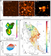 |
Fig. 1. Capabilities of the MGCLS data. Panel A: brightness cutouts from the MCXC J0027.3−5015 field, showing MeerKAT’s instantaneous sensitivity to a range of angular scales. From left to right: full-resolution (7.4″ × 7.0″), convolved 25″ resolution, and filtered ‘diffuse emission’ at 25″ resolution. The synthesised beam is shown in grey in the lower left corner of each image. The colour scale is in square root scaling in each case, with a minimum and maximum brightness of −10 and 600 μJy beam−1 (left), 6 and 400 μJy beam−1 (middle), and 25 and 150 μJy beam−1 (right), respectively. See Sect. 4.3.1 for further details. Panel B: example of an in-band spectral index map of a bent tailed source in the MCXC J0431.4−6126 field, with total intensity coloured by spectral index. The host galaxy, 2MASX J04302197−6132001, is coincident with the radio core (seen in cyan). The colour scale indicates the spectral index, and the brightness gradient of the colour bar indicates intensity, with a burned-out maximum of 10 mJy beam−1. Regions where the S/N was too low to determine a spectral index have been left white. The synthesised beam (7.1″ × 6.7″) is shown by the grey ellipse in the lower left corner. Panel C: example of an RM map of a complex MGCLS source in the Abell 3667 field. Contours are Stokes-I intensity with levels of (5, 10, 20, 40, 60, 80, 100) × σ, where σ = 6.7 μJy beam−1. To avoid including spurious RM values, pixels with Stokes-I intensity below 8σ have been masked. Panel D: H I velocity map of Minkowski’s object in Abell 194, at a resolution of 19″ × 15″ (beam shown at the top left). Contours show the integrated H I flux density at levels of (0.35, 0.7, 1.4, 2.5) mJy beam−1. Colours indicate the relative velocity from −22 km s−1 (blue) to +22 km s−1 (red) from the central velocity of 5553 km s−1. |
To exploit MeerKAT’s sensitivity to large-scale structures, without the problem of source confusion, we filter out all small-scale structure with the technique of Rudnick (2002) using a box size of 19 pixels (23.75″), and convolve the resulting ‘diffuse emission’ image to 25″. Using Fig. 3 in that paper, we can roughly quantify what percentage of the flux will be in the diffuse emission image as a function of the characteristic size of any structure. For a 60″ structure, ∼82% of the flux will be included, with higher percentages for structures of increasing sizes. Smaller scale features will be heavily suppressed, with only 5−10% of the flux remaining at 15″, and ∼0% at 8″. The result of this process is shown in the right figure of panel A in Fig. 1, where the structure of the diffuse emission is readily visible. The filtered 25″ resolution or diffuse emission maps referred to in the following sections are made using the above filtering technique. We note that these filtered maps are not included in the legacy products.
4.3.2. In-band spectral index maps
MeerKAT’s wide 0.8 GHz bandwidth in the L band allows for in-band spectral index studies, with primary-beam-corrected spectral index and associated uncertainty maps being part of the legacy products. Panel B of Fig. 1 shows an example spectral index map for a MGCLS radio galaxy with diffuse lobes. As per the caveats discussed in Sect. 4.4.2, a reliable spectral index can only be fit for pixels with S/N ≳ 10. Spectral index uncertainty maps contain only the statistical uncertainty from the fit, with constrained spectral indices typically having per-pixel statistical uncertainties between 0.05 and 0.2.
4.3.3. Polarisation studies
All of the MGCLS targets were observed in full polarisation, with 44 of the clusters being mapped in polarisation for DR1 (see Table 1 at the end of the paper for the full list). Allowing for the caveats mentioned in Sect. 4.4.5, the sensitivity of the MGCLS polarisation maps will allow for the detection and determination of RMs for a large population of radio sources. Such detections will allow statistical studies of cluster magnetic fields. The determination of RMs of extended sources at high spatial sensitivity will also allow a detailed study of magnetic field strengths and structure across various source morphologies (e.g. radio galaxies and relics). Panel C of Fig. 1 shows an RM map for one such extended source in the Abell 3667 field. This map is discussed in more detail in Sect. 6.1.3.
4.3.4. H I capabilities
In addition to the continuum and polarimetric use cases, the MGCLS visibilities can also be used for H I studies. The MGCLS frequency resolution of 209 kHz corresponds to an H I velocity resolution of 44.1 km s−1 (at z = 0). The survey is therefore suitable to approximately resolve the velocity structure of galaxies with a rotational amplitude of ≳100 km s−1 (depending on their inclination), which can be seen as a rough threshold dividing dwarf galaxies from more massive objects (Lelli et al. 2014).
The top panel of Fig. 2 shows the H I mass sensitivity as a function of redshift for an integration time of 3 and 12 h (the range of usable on-source time for H I analysis in the MGCLS, with most clusters having 6−10 h on-source), demonstrating that the MGCLS observations are able to detect galaxies below the ‘knee’ of the H I mass function ( , Jones et al. 2018) out to z ≲ 0.1. Moreover, the angular resolution provided by the survey, shown in the bottom panel of Fig. 2, enables one to resolve the structure of the H I in galaxies with a resolution between 10″ and 30″, corresponding to a spatial resolution of ∼4 − 20 kpc at redshifts of 0.02 < z < 0.1. This means that for clusters in this range, larger galaxies will be spatially resolved and we can conduct studies of resolved H I galaxies while simultaneously probing extended extragalactic structures in the wide field of view – a key discriminating feature with respect to single-dish H I surveys of rich environments. Panel D in Fig. 1 shows an example of a resolved H I detection, covering two consecutive channels, in the Abell 194 field. Examples of H I science from the MGCLS datasets are given in Sect. 9.
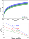 |
Fig. 2. H I mass sensitivity for the MGCLS. Top: logarithm of the total H I mass sensitivity as a function of redshift for integration times between 3 h and 12 h (not all MGCLS datasets have the same usable on-source time for H I analysis). The shaded areas indicate the H I mass limits of the MGCLS data assuming a 5σ detection for a galaxy with line width ranging from 44 km s−1 to 300 km s−1. Bottom: column-density sensitivity versus angular resolution at z = 0.03 for different integration times present in the MGCLS. The horizontal axis scale is proportional to HPBW−2. |
4.4. Data quality issues
There are a number of issues with data quality in the DR1 release that affect the visibilities and images. The images have been corrected for a number of these effects, as described below. However, they still affect the visibilities, and impose limitations on the accuracy of the images. Users of the data products should take these into consideration when scientific analyses are performed.
4.4.1. Dynamic range
Fields with very strong sources (I > few 100 s mJy beam−1) are typically limited by residual artefacts from the brighter sources. This is especially true if there are several widely separated bright sources, as the self-calibration cannot correct direction-dependent effects (DDEs). The DDEs that are thought to dominate are asymmetries in the antenna pattern, pointing errors, and ionospheric refraction.
4.4.2. Flux density and spectral index
Uncertainties in the primary beam pattern affect both the derived brightnesses and spectral indices. Near the centre of each field, the total array pattern is very close to that of the individual antennas (Mauch et al. 2020). However, application of this individual antenna pattern to spectra of sources in the outer parts of cluster fields produces non-physical results. This is expected because the array power pattern is broadened by pointing errors in the individual antennas. Derived brightnesses, and especially spectral indices, are therefore not reliable beyond a radius of 36′.
We compared the flux densities of the MGCLS compact sources with those from other radio surveys, as discussed in Sect. 5.2.1, and found them to agree to within about 6%, with the MeerKAT flux densities being, on average, 6%±4% lower than those of the other two catalogues. No corrections to the flux densities have been made in either the catalogues or the maps.
While MeerKAT’s very wide fractional bandwidth improves the sensitivity and gives us the ability to derive in-band spectral indices, it also creates uncertainties regarding the effective central frequency at each pixel. Simple averaging in frequency space would result in effective reference frequencies that depend on the spectra of the sources in question and their position in the field. When we can adequately fit the spectrum, typically requiring a S/N ≥ 10, the brightness is calculated correctly at the well-defined reference frequency of 1.28 GHz. The spectral fit was accepted if the χ2 per degree of freedom was less than 1.5 times the χ2 per degree of freedom based on assuming the default value of −0.6; otherwise the default value is reported and the central frequency brightness is calculated with that spectral assumption. This results in an underestimate of the brightness by ∼6% (10%) for a true spectral index of −1 (−2). Typically, these are less than the random errors in these low brightness cases.
Since the flux density threshold for switching to the default spectral index depends on the local noise properties of each cluster image, no global value can be specified. However, inspection of the spectral indices as a function of flux density for a selected region reveals the appropriate local threshold below which the default spectral index has been assigned. Caution is still advised when examining regions of maps where spectral indices very close to the default value are encountered.
4.4.3. Largest angular size
MeerKAT has very good short baseline coverage, allowing recovery of extended emission. However, the minimum baseline length of 29 m does restrict the maximum size of a structure that is properly imaged. This maximum size scales inversely with frequency. Angular scales of less than 10′ should be fully recovered. Larger scales are less well imaged, especially at the higher frequencies. This effect leads to negative holes around bright extended structures and an artificial apparent steepening of the spectrum. Very steep fitted spectra of extended emission should be treated with caution.
4.4.4. Astrometry
A number of instrumental issues can affect the accuracy of the astrometry. As detailed in this section, we correct the image astrometry in each field by matching the positions with those of the respective optical hosts. This results in a final accuracy better than 0.3″ in the high S/N limit. However, the astrometric errors are still present in the visibility data, and users that reprocess raw data need to take these into consideration.
Data in the earliest observations suffered from a 2-second time offset in the labelling of the data, and a half-channel frequency error, which propagate into errors in the u, v, w coordinates. The column ‘Fix’ in Table 1 indicates cluster fields where this issue was corrected in the visibilities. Fields that were not fixed will contain rotation and scaling errors in the positions of sources that depend on position in the field. These can be as large as 2″ at the edge of the fields.
Calibrator position errors were present in the initial MeerKAT calibrator list, affecting several calibrators up to a level of several arcseconds. This results in an approximately constant position offset of sources in the affected cluster fields. Corrections were made in the images when incorrect calibrator positions were discovered, but the final corrections were made at the end, in any case, through optical cross-matching.
A low-accuracy delay model in the correlator in use during the observations can cause a similar, albeit subtler, problem when the calibrator and target are widely separated. An additional bias is possible when the calibrator does not sufficiently dominate the visibility intensities in the field. The model had insufficient accuracy to reliably transfer phases measured on the calibrator to those of the target, especially since many of the astrometric calibrators were 10° or more from the target. This resulted in approximately constant position offsets of up to several arcseconds in individual fields, which had to be corrected.
Astrometric corrections were made for each field centre, removing or reducing the effects noted above. We matched compact radio components to a large number of background quasars, radio galaxies, and star-forming galaxies in each field, using the optical and infrared catalogues from the Dark Energy Camera Legacy Survey (DECaLS; Dey et al. 2019). A flux density-weighted average correction was determined for every cluster field, as indicated in column ‘Posn’ in Table 1, and appropriate corrections made to each corresponding image. Residual systematic errors should be under 0.1″ for clusters as a whole, although errors may be larger for individual sources.
Additional astrometric checks were carried out after the above correction by cross-matching with sources from the International Celestial Reference Frame (ICRF) catalogue (Charlot et al. 2020). Since the ICRF constitutes the most accurately known set of astronomical positions, they are an ideal check of the astrometry in the MGCLS catalogue described in Sect. 5.2. There are eight ICRF sources in our cluster fields. They are bright (0.3 to 1.8 Jy), and the statistical uncertainty in their MeerKAT position determinations are therefore small. They were chosen for the ICRF for being compact on milliarcsecond scales, and they generally do not have structure on the MeerKAT’s ∼8″ scale, which might affect the position determination. We therefore compared our catalogue positions with the ICRF38 ones for the eight sources that were included in our fields: ICRF J010645.1−403419, J025612.8−213729, J031757.6−441417, J033413.6−400825, J060031.4−393702, J062552.2−543850, J124557.6−412845, and J133019.0−312259.
We found that most of the MGCLS catalogue positions differed from the ICRF3 ones by less than 1″ in either coordinate. The single exception was ICRF J025612.8−213729 (QSO B0253−218) for which the MGCLS catalogue position was ∼2.3″ north of the ICRF3 position. This source is an exception to the above generalisation about lack of structure, in that Reid et al. (1999) show it to be somewhat extended in a N–S direction at 5 GHz, with several components spread out over ∼10″. This field, MACS J0257.6−2209, is also one of the few for which there were uncorrected timing and frequency errors (Col. 5 in Table 1, discussed earlier in this section) that will cause position errors far from the field centre. In addition, since the source is resolved, the MGCLS position at 1.28 GHz and ∼8″ resolution could differ from the ICRF3 position, which is that of the milliarcsecond core only at 5 GHz.
Ignoring this source, we find that for the remaining seven sources the difference between the MGCLS catalogue positions and the ICRF3 ones were −0.04 ± 0.34″ in RA and −0.02 ± 0.15″ in Dec. This check gives us confidence that the positions in the MGCLS catalogue are accurate, and adopt the uncertainty of 0.36″ based on the ICRF3 comparisons.
4.4.5. Polarisation
The first plane of the Stokes Q and U5pln cubes (see Sect. 4.2.1) provide a good indication of where significant polarisation is present, but should not be used quantitatively on their own. Each image was created by a noise-weighted sum of the frequency planes in the full cube, which is strictly correct only when both the RM and the spectral index are zero, and when no depolarisation is present. At any RM ≠ 0, the amplitude of Q and U will be reduced, reaching a factor of 2 reduction at |RM|∼25 rad m−2, depending on the source spectral index and the noise in the different frequency channels. The first plane of the Stokes Q and U5pln cubes should therefore be used quantitatively with caution.
We note that polarisation leakage affects the upper half of the band, with the residual polarisation leakage increasing with distance from the field centre within the half-power region of the beam (de Villiers & Cotton, priv. comm.; de Villiers et al. 2021). The instrumental polarisation may reach up to 10% in the upper part of the band, while it is typically less than 2% at the lower frequencies. Users should evaluate how the leakage affects their particular science case.
5. MGCLS source catalogues
We produced source catalogues for all fields in the MGCLS, based on the intensity plane of the full-resolution enhanced products described in Sect. 4.2. Here we detail our source finding method, as well as the various catalogues being provided with the legacy data products. Limitations to the accuracy of the results are discussed in Sect. 4.4. It is very important to note that these catalogues are not complete, and any statistical analyses must consider their limitations. In particular, the sensitivity depends on the distance from the respective field centres, and regions around bright sources are excluded, as discussed below.
5.1. Source detection
We used the Python Blob Detection and Source Finder (PYBDSF; Mohan & Rafferty 2015) software to create individual source catalogues for all MGCLS fields, using the full-resolution, primary-beam-corrected data products. PYBDSF searches for islands of emission and attempts to fit models consisting of one or more elliptical Gaussians to them. Gaussians are then grouped into sources, and there may be more than one source per island. Each source is given a code: ‘S’ for single-Gaussian sources that are the only source on its island, ‘C’ for single-Gaussian sources that share an island with other sources, and ‘M’ for sources composed of two or more Gaussian fits. We used the default 3σimg island boundary threshold and 5σimg source detection threshold, where σimg is the local image rms. As many images have variable image noise levels across the field, we allow PYBDSF to calculate the 2D rms map during the source finding.
For sources in regions of high image noise, for example those near bright sources with strong sidelobes, the typical statistical uncertainty in peak source brightness is a factor of ∼2 larger than for sources elsewhere in the same field. Spurious source detections are common around very bright sources, with PYBDSF sometimes cataloguing sidelobes as sources. To mitigate spurious detections in our DR1 catalogues, we excised all catalogue entries around bright sources. A source was considered bright if its peak brightness was higher than the bright source limit for that field,  . This limit is connected to the image dynamic range, such that
 (2)
(2)
where Imax is the maximum source brightness in the image, and σglobal is the median image rms, both in units of Jy beam−1. The region around a bright source within which catalogue entries were excised, rcut, scales with the source brightness:
 (3)
(3)
where both  and
and  , the peak brightness of the bright source, are in Jy beam−1. A median of 2.6% of nominally detected sources were removed per field through this process.
5.2. Compact source catalogue
From our PYBDSF results, we compiled a single MGCLS compact source catalogue from all fields, only including sources that could be fit with a single Gaussian component (source codes ‘S’ or ‘C’), after the spurious source excision. The full DR1 catalogue9 contains ∼626 000 sources from the 115 cluster fields, with an excerpt shown in Table 2. The catalogue columns, described in the Table caption, contain standard radio source information including the integrated flux density, peak brightness, and source size, with catalogue source positions provided in decimal degrees. The source identifier (first column of the catalogue) uses an International Astronomical Union (IAU) classification, with the designation MKTCS JHHMMSS.ss±DDMMSS.s, where the decimal positional information is truncated, rather than rounded.
Excerpt of the MGCLS compact source catalogue at 1.28 GHz.
5.2.1. Comparison with previous radio catalogues
To verify the MGCLS compact source flux densities, we compare them to those from other radio surveys. To cover all MGCLS pointings, we use catalogues from both the 1.4 GHz NRAO VLA Sky Survey (NVSS; north of −40° Dec; Condon et al. 1998) and the 843 MHz SUMSS survey (south of −30° Dec; Bock et al. 1999). To scale the NVSS and SUMSS flux densities to the MGCLS reference frequency of 1.28 GHz, we assume a power law Sν ∝ να with a fiducial spectral index of α = −0.7 (Smolčić et al. 2017).
To avoid incompleteness effects due to differences in sensitivity between the three surveys, we consider only sources with S/N ≥ 50 in all three surveys. This high limit also minimises effects from additional faint MGCLS sources within the larger NVSS and SUMSS beams, as noted below. To cross-match MGCLS compact sources with their NVSS and SUMSS counterparts, we use a 5″ radius. This radius is a compromise between maximising the number of real counterparts and minimising the number of spurious matches. By shifting the MGCLS sources by 1′ and repeating the cross-matching, we determine that the expected percentage of spurious matches is 4.1% and 3.8% for NVSS and SUMSS, respectively. These have a negligible effect on the flux density comparisons.
Our cross-matching yields a total of 398 and 565 compact MGCLS sources with NVSS and SUMSS counterparts, respectively. Figure 3 shows the flux density scale comparison between the MGCLS compact sources and the scaled NVSS (top panel) and scaled SUMSS (bottom panel) sources. The MGCLS flux densities are in good agreement with those of both NVSS and SUMSS. We fit a power law of the form
 (4)
(4)
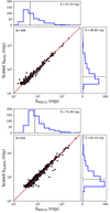 |
Fig. 3. Comparison between the integrated flux density of MGCLS compact sources with their counterparts in the NVSS (top) and SUMSS (bottom) catalogues, with the latter two being scaled to the MGCLS frequency of 1.28 GHz. The best-fit relation in each case is shown by the solid red line and is consistent with a linear relationship, with the number of sources in the fit shown in the upper left corner. The dashed grey line shows the exact one-to-one relationship. The scaled sky survey flux densities are typically 6% higher than their MGCLS counterparts, so this represents a possible small bias in the MGCLS flux scale. Histograms show the relevant flux density distributions, with the dashed black lines indicating the respective median values, |

to the MGCLS and scaled NVSS and SUMSS flux densities. Values of 1 for both κ and γ would indicate an exact one-to-one correspondence. We obtain fit values of κNVSS = 1.06 ± 0.02, γNVSS = 1.00 ± 0.01, and κSUMSS = 1.06 ± 0.04, γSUMSS = 1.00 ± 0.01 for the NVSS and SUMSS comparisons, respectively. This is consistent with a linear relation between the MGCLS and scaled fluxes, with the scaled NVSS and SUMSS fluxes being marginally higher than those from MGCLS. The MGCLS sources were not chosen to be isolated, so the poorer resolution of the sky surveys (∼45″) may lead to a single NVSS or SUMSS source having contributions from additional faint MGCLS sources; at the lowest fluxes, this could result in a small bias in opposite spectral index directions for the two surveys. However, the equality of the fitted flux densities show that any such effects are negligible.
We also examine the spectral index distribution of the radio cross-matched MGCLS compact sources. For this purpose, we include 148 MHz data from the TIFR GMRT Sky Survey (TGSS; north of −53° Dec; Intema et al. 2017) in addition to the NVSS and SUMSS surveys. Given the different sky coverages, some MGCLS sources have flux densities at only one additional frequency, whereas others have three. We fit a single Sν ∝ να power-law and inspected each fit to discard both spurious matches and sources showing spectral curvature. Figure 4 shows the resulting spectral index distributions. The distributions of spectral indices for sources with two, three, and four frequency points are similar, although the Nν = 4 distribution has a lower median spectral index. Subtle differences may reflect differences in the spectral populations of the different surveys, but are beyond the scope of the current work.
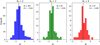 |
Fig. 4. Spectral index distributions for the cross-matched MGCLS compact sources, using data from the MGCLS (1.28 GHz), NVSS (1.4 GHz), SUMSS (843 MHz), and TGSS (148 MHz) catalogues. Left to right: distributions for MGCLS sources with flux density measurements at two, three, and four frequencies, respectively. The number of compact sources, Ns, and the median spectral index, |

5.2.2. Optical cross-matching
We created optical cross-match catalogues for the compact sources in the Abell 209 and Abell S295 fields using data from DECaLS (Dey et al. 2019). These fields were selected due to their existing DECaLS coverage and their decent MGCLS dynamic range. Cross-match catalogues for other MGCLS fields will be compiled in follow-up works.
To identify DECaLS counterparts for the MGCLS compact sources, we used the likelihood ratio (LR) method (Sutherland & Saunders 1992; Laird et al. 2009; Smith et al. 2011). The LR here is defined as the ratio of the probability that an optical source (at a given distance from the radio position and with a given optical magnitude) is the true counterpart, to the probability that the same source is a spurious alignment, that is, LR = (q(m)×f(r))/n(m), where q(m) is the expected number of true optical counterparts with magnitude m, f(r) is the probability distribution function of the positional uncertainties in both the radio and the optical source catalogues, and n(m) is the background density of optical galaxies of magnitude m in the DECaLS r band (or g or z band). The magnitudes are AB magnitudes from DECaLS DR8.
The a priori probability q(m) is determined as follows. First, the radio and optical source catalogues are matched by finding the closest counterpart within a fixed search radius of 4″. We chose this radius based on our distributions of cross-matches, as shown in Fig. 5, where the distributions (LR > 0.5) of the RA and Dec angular separations between the positions of radio sources can be approximated by Gaussians. The search radius of 4″ is the optimal radius where we detect the most true sources. Radii greater than 4″ will sharply increase the number of spurious matches. The number of spurious matches (of magnitude m) is estimated by scaling n(m) to the area of 4″ radius within which we search for counterparts. This is then subtracted from the number of counterparts (as a function of magnitude) to determine the number of true associations, q(m).
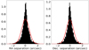 |
Fig. 5. Histograms of the RA and Dec angular separations between the positions of radio sources in the Abell 209 compact source catalogue and their optical counterparts, for LR > 0.5. In each panel, the red line shows the normalised Gaussian distribution. |
In our case, the probability distribution f(r) is a two-dimensional Gaussian distribution:
 (5)
(5)
Here, r is the angular distance (in arcsec) from the radio source position, and δ is the combined positional error given by  , where δdecals is the positional uncertainty from the DECaLS catalogue, and δmgcls is the positional uncertainty from the MGCLS compact source catalogue. For each source in the MGCLS DR1 compact source catalogue, we adopted an elliptical Gaussian distribution for the positional errors, with the uncertainties in RA and Dec on the radio position reported in the radio catalogue. We assume a systematic optical position uncertainty of 0.2″ in both RA and Dec for the DECaLS catalogue (Dey et al. 2019).
The optical cross-match catalogue includes all matches within 4″ of a compact MGCLS source detection, along with their LR probabilities and flags (no LR cutoff imposed). Table 3 shows an excerpt from the optical cross-match catalogue for the Abell 209 field, with the full catalogues for it and the Abell S295 fields available online10. The presence of more than one counterpart for a particular radio source provides additional information to that contained in the LR itself, which can then be used to estimate the reliability of the counterpart source, or the probability that a particular source is the correct counterpart. The reliability for radio source i, as defined by Sutherland & Saunders (1992), is calculated as
 (6)
(6)
Excerpt of the compact source catalogue for Abell 209 with optical cross-match information from DECaLS.
where ∑LRsearch radius is the sum of LR for all possible DECaLS counterparts to the radio source within our search radius of 4″, and Q is the fraction of MGCLS compact radio sources with optical counterparts above the DECaLS magnitude limit. Comparison of ∑RELi with the total number of counterparts with LR > LRcutoff provides an estimate of the spurious identification rate, or error rate (ER). The choice of the cutoff in LR is a trade-off between maximum completeness and maximum purity. Completeness is defined as the fraction of radio catalogue sources that have an optical counterpart, and purity (given by 1 – ER) is the fraction of radio-optical source matches that are real.
Figure 6 shows the completeness and purity for both Abell 209 and Abell S295, with no LR cutoff imposed. Our chosen LRcutoff of 0.5 is indicated by the vertical dotted line. A value of LRcutoff = 0.5 corresponds to an estimated spurious identification rate of 4.5% in Abell 209, with 59% (2723 of 4581) of radio sources in the Abell 209 compact source catalogue having optical counterparts.
 |
Fig. 6. Completeness (left axis, solid lines) and purity (right axis, dashed lines) versus the LR for Abell 209 (black) and Abell S295 (red). Imposing a LR cutoff at 0.5 (vertical dotted line) for Abell 209, the estimated spurious identification rate (error rate, or 1 – purity) is 4.5%, with a completeness of 59%. |
5.3. Extended sources
We do not provide catalogues for the extended sources, that is, those for which the PYBDSF fit required multiple Gaussians, indicated in the PYBDSF output with code ‘M’. These need to be verified visually, a process that is extremely time consuming. However, to provide an indication of the number of extended sources in the MGCLS, we performed this verification for sources in the Abell 209 and Abell S295 fields.
Extended sources can be separated into two categories: blended sources (i.e. those with overlapping Gaussian components) and multi-component sources with multiple, non-overlapping, and often visually separable components. There are 158 and 347 blended sources in the Abell 209 and Abell S295 fields, respectively, roughly 3−5% of the number of compact sources in the respective fields. Their integrated flux densities range from 85 μJy to 105 mJy, with the largest blended sources being just over 30″ across. Extrapolating these numbers to the full MGCLS sample, there are of the order of 29 000 blended sources in the full survey.
We defined the multi-component sources as those with distinct structures such as jets, cores, or lobes. Identifying the different components that comprise a single source can be difficult, and is still typically done through visual inspection. Automated methods, such as those discussed in Appendix C, will be needed as our datasets become larger and larger. We visually inspected the Abell 209 and Abell S295 fields, finding 33 and 26 multi-component sources in each field, respectively. The largest of these multiple-component sources spans an angular size of 9.8′. For each source we measured the integrated flux density, including all components, using pixels above 3σ, where σ is the local rms. Catalogues of these sources are presented in Tables A.1 and A.2, which include the likely optical or infrared counterpart from either the DECaLS or Wide-field Infrared Survey Explorer (WISE, Wright et al. 2010) catalogues. The catalogue position for each extended radio source is fixed to that of its likely optical or infrared counterpart, if available, or otherwise given by the flux-weighted centroid.
Due to the combination of high sensitivity and resolution, many well-resolved and multi-component radio galaxies have contaminating foreground or background sources that can currently only be separated visually, if at all. Figure 7 shows one example of a giant radio galaxy (Colafrancesco et al. 2016; Kuźmicz et al. 2018) in the Abell 209 field. This ∼7.7′ structure appears to have several possible optical or infrared counterparts, all of which are associated with compact radio features. The left-most green circle in Fig. 7 indicates the position of WISE J013313.50−130330.5, a candidate quasar (Flesch 2019) at a redshift of z = 0.289 and the likely counterpart for the giant radio galaxy. At that redshift, the radio galaxy extent would be > 1.5 Mpc. The right-most green circle is associated with WISE J013259.20−130002.0, which has no available redshift. It appears to be a distorted bent-tail source whose features merge (in projection) with those of the western lobe of the assumed giant radio galaxy. Spectral index studies and redshift measurements will likely to be needed to disentangle such structures (Mhlahlo & Jamrozy 2021), which appear frequently in the MGCLS images, due to the high sensitivity to extended structures.
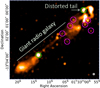 |
Fig. 7. Full-resolution (7.6″ × 7.4″) MGCLS Stokes-I intensity image of a multi-host structure in the field of Abell 209. We indicate the two possible intersecting multi-component radio galaxies (giant radio galaxy and a distorted tailed galaxy). The compact radio components circled in green indicate the positions of the likely optical hosts, while the magenta circles indicate other superposed or nearby compact radio emission with optical counterparts. The brightness scale is logarithmic and saturates at 1 mJy beam−1. The synthesised beam is indicated in the lower right corner. |
6. MGCLS diffuse cluster emission
A key aspect of radio observations of galaxy clusters is the detection of diffuse cluster-scale synchrotron emission, which carries information about the cluster formation history (see van Weeren et al. 2019; Brunetti & Jones 2014, for observational and theoretical reviews, respectively). There are several different categories of diffuse cluster radio emission, historically separated into three main classes: radio halos, mini-halos, and radio relics. All classes are characterised by low surface brightness and, typically, steep radio spectra (α ≲ −1.1).
Radio halos are diffuse sources that cover scales greater than 500 kpc, with many spanning megaparsec scales. They are typically seen to have morphologies closely linked to those of the X-ray emitting ICM. Both individual studies (e.g. Brunetti et al. 2001; Lindner et al. 2014) and statistical studies of large samples (Cassano et al. 2013; Kale et al. 2015; Cuciti et al. 2021a) have shown a strong link between radio halos and particle re-acceleration following major cluster mergers, as well as correlations between source radio power and cluster mass and thermal properties.
Radio mini-halos are found in the central region of dynamically relaxed, cool-core clusters (see Giacintucci et al. 2017, for a recent update). They are defined to be smaller than radio halos, with projected sizes ranging from a few tens of to a few hundred kiloparsecs, usually confined within cold fronts at the cluster centre (Mazzotta & Giacintucci 2008). Mini-halo clusters always have a radio active brightest cluster galaxy (BCG), which is thought to provide at least a fraction of the seed electrons necessary to produce the diffuse emission (see e.g. Richard-Laferrière et al. 2020). Particle re-acceleration induced by gas sloshing is possibly the driving mechanism for mini-halos (e.g. ZuHone et al. 2011, 2013).
Radio relics are elongated megaparsec-scale structures located at the periphery of merging galaxy clusters. Their observed properties, which include a high degree of polarisation (see for instance the case of the Sausage cluster, van Weeren et al. 2010) are consistent with the idea that they are related to the presence of merger-induced shocks in the ICM. Double radio relics are found in a number of clusters, the prototype case being Abell 3667 (Rottgering et al. 1997), and in some cases a radio halo is detected as well (see e.g. Bonafede et al. 2012; Lindner et al. 2014). Radio phoenix sources are a sub-class of relics thought to be related to revived fossil emission from radio AGN in the cluster region (van Weeren et al. 2019).
Radio halos and relics have been detected in an increasing number of merging clusters, over a broad range of cluster masses (see van Weeren et al. 2019; Cuciti et al. 2021b, for recent updates) and over a wide range of redshifts (Lindner et al. 2014; Di Gennaro et al. 2021). The detection of mini-halos, by contrast, remains limited, mainly due to observational constraints. In addition to the three main classes, more clusters with very steep-spectrum filaments have been detected recently (e.g. Abell 2034, Shimwell et al. 2016), requiring further investigation of the connection between the structures and particle reservoirs radio galaxies deposit into the ICM, and the effects of cluster merger events (see e.g. van Weeren et al. 2017; de Gasperin et al. 2017).
Of the 115 clusters observed in this Legacy Survey, 62 have some form of diffuse cluster emission, with several clusters hosting more than one diffuse source. Table 4 presents the list of all 99 diffuse cluster structures or candidates detected in the survey. Fifty-six of these are new. For each diffuse source we list the emission classification, as well as angular and physical projected sizes, and position relative to cluster centre (where relevant). Classifications are based on a combined interrogation of the full- and 15″ resolution MeerKAT data products, a 25″ resolution filtered image (see Sect. 4.3.1 for details), and any available optical and X-ray imaging. Candidate structures are those with either marginal detections or where the classification is uncertain. Where a diffuse source does not fit into any of the current classes, but is not clearly associated with an individual radio galaxy, we classify it as ‘unknown’. Our diffuse cluster emission detections can be summarised as follows: three new mini-halos and seven new mini-halo candidates, 27 halo detections and six candidates (of which 13 are new), 28 relics and 18 candidates (of which 26 are new), one known phoenix source and two new candidates, and nine diffuse sources, six of which are new, with ambiguous or unknown classifications.
Catalogue of the 99 diffuse cluster radio sources detected in the MGCLS.
The galaxy clusters observed in the MGCLS provide just a glimpse of the many diffuse cluster emission discoveries likely to be made in the Square Kilometre Array era. In the following, we present a few examples to show the much improved images compared to previous observations, opening up new areas of investigation, as well as discoveries highlighting specific interesting science issues. Flux densities for the diffuse emission in these systems have been measured by integrating the surface brightness within the 3σ contour in the 15″ resolution image and then subtracting the compact source contributions, which are determined from the full-resolution image. In some cases the 25″ resolution filtered image shows a greater extent to the diffuse structures than the 15″ resolution products; the flux densities quoted here may be considered as lower limits to the total amount of diffuse emission.
6.1. New insights into known sources
Twenty-eight of the MGCLS targets are hosts of previously known diffuse cluster emission. In many cases the MGCLS data provide an additional frequency or deeper detections of low-surface-brightness emission, yielding new insights into well-known sources (e.g. El Gordo, Abell 3376). Here we provide three examples.
6.1.1. Abell 85: A new type of halo?
The MGCLS multi-resolution view of the Abell 85 system, a cool-core cluster at z = 0.0556 and part of the Pisces-Cetus supercluster, is shown in the top panel of Fig. 8. We detect two diffuse sources: a complex phoenix or revived fossil plasma source south-west of the cluster centre (previously known) and a newly discovered elongated radio mini-halo that may be an example of a new class of sources that represents an evolutionary bridge between mini-halos and halos.
 |
Fig. 8. Multi-resolution MGCLS view of Abell 85. Top: full-resolution (7.7″ × 7.1″; yellow, log scale between 0.006 and 2 mJy beam−1) and filtered 25″ resolution (blue, log scale between 0.06 and 3 mJy beam−1) Stokes-I intensity image of Abell 85, with the bright BCG and tailed radio galaxy emission filtered out. Smoothed archival Chandra 0.5−7 keV X-ray contours (levels: 1.0, 1.7, 3.4, 6.8, 13.6 × 10⁻⁷ counts cm−2 s−1) are overlaid in white. The respective synthesised MGCLS beams are shown on the lower left. The physical scale at the cluster redshift is indicated on the upper left, and the red × marks the NED cluster position. A newly detected elongated mini-halo (largest linear size ∼370 kpc) is seen around the cluster BCG. Filamentary structures are seen in the known phoenix/revived fossil plasma source SW of the cluster. Bottom: Pan-STARRS r-band images of the boxed regions from the top panel, with MGCLS 15″ resolution contours overlaid. Contour levels start at 3σ = 30 μJy beam−1 and increase by factors of 3. |
The newly detected diffuse source in Abell 85 surrounds the BCG, with contours shown in panel A of Fig. 8, and has a 1.28 GHz flux density of ∼5.5 mJy measured from the 15″ resolution image. The 25″ resolution image, also shown in Fig. 8, reveals a much greater extent to this source, with a largest angular size of 5.6′ (∼370 kpc). This structure has not been detected in any of the low resolution radio data available in the literature at other frequencies (see Duchesne et al. 2021a, and references therein), possibly due to its low surface brightness (∼1.1 μJy arcsec−2 in the diffuse emission filtered 25″ resolution image) and its proximity to the 27 mJy BCG and 13 mJy tailed source. Given its size and location in a cool-core system, we classify this new detection as a mini-halo. We note, however, that the MGCLS contains discoveries of several other examples of elongated diffuse halos with embedded central radio-loud BCGs (indicated by ( † ) in Table 4 at the end of the paper), some of which are on megaparsec scales. We may be observing a new type of diffuse structure, bridging both halo and mini-halo classifications. A handful of cool-core clusters have been found to host larger scale radio halos (Bonafede et al. 2014; Sommer et al. 2017), and in each case the cluster shows signs of merger activity in addition to the cool X-ray core, as is the case for Abell 85 (Yu et al. 2016).
The phoenix source has been studied at multiple frequencies (Slee & Reynolds 1984; Slee et al. 1994, 2001; Giovannini & Feretti 2000; Duchesne et al. 2021a), variously classified as a revived fossil plasma source, a phoenix, and a relic. At full resolution (yellow in Fig. 8), MeerKAT images this source in unprecedented detail, resolving a large number of filamentary structures extending from a brighter complex core region. At the filtered 25″ resolution (blue in Fig. 8) we recover the full angular extent of the source as seen at lower frequencies (Duchesne et al. 2021a). The diffuse emission extends far from the filaments, suggesting that some form of distributed re-acceleration is necessary.
The source’s complex morphology could result from recurrent episodes of AGN activity, although determining the host galaxy(ies) for these structures is not trivial. Several potential hosts can be seen in the Pan-STARRS r-band image in Fig. 8. Sub-arcsecond resolution imaging is needed to identify the radio core(s), if present, in order to cross-match with optical counterpart(s). The toroidal structure in the western region of the source may indicate late stage radio-mode feedback in a non-central cluster galaxy source (such as in M 87, Nakamura & Asada 2013; Walker et al. 2018), possibly caused by an evolved radio lobe that has been transformed into a ‘smoke-ring’-like feature (Enßlin & Brüggen 2002). Such vortex structures can travel much further than amorphous plasma structures can, as shown by hydrodynamical simulations (Turner & Taylor 1957), and the radio features here could therefore be at a more advanced stage than the radio emission in M 87. The buoyancy produced by this off-centre bubble is sufficiently powerful to uplift the ICM, visible in the Chandra X-ray contours in Fig. 8. Filamentary wings of radio emission trail the bubble for about 200 kpc (at the cluster redshift). The filaments are quite narrow (10−20 kpc), which constrains transport parameters for the enclosed cosmic-ray electrons, as well as ambient turbulent motions that would disrupt such structures (de Gasperin et al. 2017). Such filaments can survive in turbulent motions provided that there are Reynolds stresses of magnetic fields that thread the wings (Banda-Barragán et al. 2018). Determining the Alfvén scale – the physical scale at which the magnetic tension starts to play a role in turbulent dynamics – may assist in clarifying their role.
Spectral information can help constrain the history of the cosmic-ray population in the phoenix source. From the full source volume, we measure a flux density of S1283 MHz = 242.4 ± 12.1 mJy. Comparing to a flux density of S148 MHz = 9.82 ± 0.98 mJy within the same solid angle from TGSS (Intema et al. 2017), we obtain a steep integrated spectrum of  for the full source. This latter value is in agreement with the 148−300 MHz spectral index of −1.85 ± 0.03 derived by Duchesne et al. (2021a). The brightest regions of the complex structure have sufficient S/N across the MeerKAT bandwidth to determine in-band spectral indices, and we find values11 ranging from −2.9 to −3.5. The steep spectra of the diffuse and filamentary structures indicate old electron populations; however, the cause of the extreme steep spectrum in the central regions is unclear. There may be an artificial steepening effect from the frequency-dependent uv-coverage; although this should not be important in the brightest fine scale structures, this requires further investigation.
6.1.2. RXC J0520.7−1328: Revealing a diffuse multiplex
The MGCLS reveals complex structures in the previously studied cluster RXC J0520.7−1328 (also known as MACS J0520.7−1328, Ebeling et al. 2001) that do not obviously fit any of the existing paradigms. RXC J0520.7−1328, at z = 0.336, is part of a possible cluster pair, with its companion, 1WGA J0521.0−1333, lying to the south-east at a redshift of z = 0.34 (Macario et al. 2014). Multi-resolution MGCLS images of this pair, presented in Fig. 9, show a large, complex, diffuse source south-east of RXC J0520.7−1328, coincident in part with 1WGA J0521.0−1333. The brightest portion of the radio emission is a bar-like feature seen at both full (8.6″; yellow) and 25″ (blue) resolution, at the south-east edge of 1WGA J0521.0−1333’s X-ray emission. This feature was observed with the GMRT at 323 MHz (Macario et al. 2014), along with three other distinct regions of faint diffuse emission (labels D2 to D4 in Fig. 9, taken from Macario et al. 2014). Although characterised as a relic by Macario et al. (2014), the bar’s south-west end is significantly brighter in the full-resolution MeerKAT image than the rest of the feature, and could instead be a head-tail galaxy. Although no MeerKAT polarisation maps are available for this system, spatial spectral index studies may be able to disentangle these two possibilities.
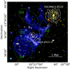 |
Fig. 9. MGCLS full-resolution (8.6″; yellow) and diffuse emission filtered 25″ resolution (blue) Stokes-I intensity image of a portion of the RXC J0520.7−1328 field, showing complex extended emission within the region. The corresponding synthesised beams are shown on the lower left by the filled yellow and blue ellipses, respectively. The colour scales are in square root scaling between 10−500 μJy beam−1 (yellow) and 20−500 μJy beam−1 (blue). The physical scale at the cluster redshift is indicated on the lower right, and the cross marks the NED cluster position. Smoothed archival Chandra 0.5−7 keV X-ray contours (levels: 3, 6, 12, 24 × 10−8 counts cm−2 s−1) are overlaid in white, with RXC J0520.7−1328 and its companion cluster 1WGA J0521.0−1333 labelled. Dashed green ellipses indicate the regions of diffuse emission, D1 to D4, identified in Macario et al. (2014). The full-resolution MGCLS image contains artefacts that radiate from the bright compact source in RXC J0520.7−1328. |
The filtered 25″ resolution MGCLS image shows that the bar-like feature is connected to two other low-surface-brightness structures: a filled circular ‘bubble’ overlapping the south-east region of 1WGA J0521.0−1333, coincident with the 323 MHz D4 source, and a partial ring or arc of radio emission lying between the two clusters (incorporating sources D2 and D3). MeerKAT reveals much more detail and extent to the complex emission seen at lower frequency. It also reveals a new faint structure (∼0.8 μJy arcsec−2 surface brightness) to the east of RXC J0520.7−1328. Despite the improved sensitivity, due to the location and morphology of the structures, it remains difficult to classify the majority of the emission in terms of typical cluster-related nomenclature. A more detailed analysis, including deeper X-ray data, polarimetry, and spectral index studies, will be required to resolve the nature of this emission.
6.1.3. Abell 3667: Polarisation with MGCLS
Radio relics are among the most polarised radio sources known, reaching 70% polarisation levels in localised regions (van Weeren et al. 2010; Loi et al. 2017). Here we showcase the MGCLS dataset’s ability to probe polarisation structure in diffuse sources on ∼10″ scales by presenting initial results from polarised observations of the north-west radio relic in the Abell 3667 galaxy cluster (z = 0.056). This relic is one of the most impressive examples of radio emission generated by a merger shock wave (Rottgering et al. 1997; Johnston-Hollitt 2003). The shock wave propagates in the ICM with a speed of 1200 km s−1, at roughly two times the sound speed (Finoguenov et al. 2010). The polarisation is maximal close to the shock front, as well as in other regions of the radio relic where the magnetic field is likely compressed and aligned by the action of the shock wave (Ensslin et al. 1998).
In Fig. 10 we see that the magnetic field appears aligned with the NW edge of the radio relic at the location of the shock; this is seen in other radio relics as well (see e.g. van Weeren et al. 2010; Ozawa et al. 2015). We also observe a patchy, disordered structure to the magnetic field away from the edge; this is seen in other relics, and is expected as turbulence develops post-shock (Kang 2017). In Abell 3667, we can rule out disorder due to Faraday rotation in the ICM since we removed these effects using the RMs shown in panel C of Fig. 1. At the same time, the RM is seen to increase from the north towards the central regions of the relic; this could be due to the sub-cluster identified in that region with X-ray observations (Finoguenov et al. 2010), if it is located in front of the radio emitting plasma.
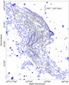 |
Fig. 10. Inferred magnetic field angles for the north-west relic in Abell 3667, after correction for Faraday rotation (which is shown in Fig. 1). Blue contours show the full-resolution (7.5″ × 7.4″) Stokes-I MGCLS intensity, with the synthesised beam shown in the boxed region on the lower left. Contour levels are 10, 20, 40, 60, 80, 100 × 1σ, where σ = 6.7 μJy beam−1. Magnetic field vectors (angles only) are shown where the linearly polarised intensity is > 8σ. The magnetic field is highly ordered along the NW edge of the relic. |
6.2. New clusters with diffuse emission
There are 34 MGCLS clusters in which we detect cluster diffuse emission for the first time. Here we present three examples that raise interesting science issues and showcase the capabilities of the MGCLS.
6.2.1. J0352.4−7401: Multiple relics in a massive merger
The MGCLS has detected several new relics, many with large-scale filamentary structure. One such example is the newly detected SE relic in MCXC J0352.4−7401 (Abell 3186, z = 0.1270) shown in Fig. 11. The relic, located approximately 1.2 Mpc SE of the cluster centre, is very large, 2 Mpc long and 340 kpc wide. The brightest region of the SE relic is a straight bar, aligned N–S and spatially connected to a 3 mJy compact source (marked by the black cross). No optical counterpart is visible in the Digitized Sky Survey (DSS). The in-band spectral index map of the SE relic, also in Fig. 11, shows this compact source to have a significantly flatter spectrum (α ∼ −0.4) than that of the bar (α ∼ −1.0 to −1.2). The overall shape of the relic is curved, with the southern part consisting of two parallel filaments with complex structure. The filaments have steeper spectra than the northern bar, with in-band spectral indices of −1.5 at the centre of the filaments, steepening to −2.5 at the edges. The trailing edge of the relic is much wider in 25″ resolution imaging of the field (shown in blue in the top panel of Fig. 11), with a maximum width of ∼580 kpc. The SE relic has a measured 1.28 GHz flux density of ∼65 mJy, which corresponds to a total radio power of P1.28 GHz ∼ 2.8 × 1024 W Hz−1.
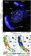 |
Fig. 11. MGCLS view of the newly detected multiple-relic and radio halo system in MCXC J0352.4−7401. Top: MGCLS full-resolution (7.0″ × 6.8″; yellow) and filtered 25″ resolution (blue) Stokes-I intensity images. The colour scales are in square root scaling between 50−500 μJy beam−1 (yellow) and 5−300 μJy beam−1 (blue). Synthesised MGCLS beams are shown on the lower right, and the physical scale at the cluster redshift is shown on the upper left. The red × marks the NED cluster position, and the black cross indicates the position of a 3 mJy compact source coincident with the SE relic. Smoothed archival Chandra 0.5−7 keV contours (levels: 4, 8, 16, 30 × 10−7 counts cm−2 s−1) are overlaid in white. Bottom: in-band spectral index (left) and spectral index uncertainty (right) maps of the dashed region from the top panel, with 15″ resolution MGCLS intensity contours overlaid. Contours start at 5σ = 40 μJy beam−1 and increase in factors of 4. The synthesised beam is indicated by the filled grey circle on the lower right of each panel. |
This system also hosts a smaller 1.1 Mpc relic north of the cluster, as well as a large radio halo that fills the X-ray emitting region. The N relic has two components in the full-resolution image and its morphology is strikingly linear, reminiscent of revived radio galaxies, although no obvious optical counterpart is seen in DSS images. Both the SE and N relics lie far beyond the observed thermal ICM (shown by white Chandra contours in Fig. 11). The large-scale radio halo, with a 1.28 GHz flux density of ∼20 mJy, lies at the centre of the cluster, and its SE–NW elongated morphology closely follows that of the X-ray emission. This giant radio halo, with a largest linear size of 1.5 Mpc, has a faint (∼0.2 μJy arcsec−2) diffuse arc-like protrusion off its NW edge, mirroring the SE relic. As the shape and position of the arc-like structure may hint at the presence of another shock front, we classify it as a candidate relic.
The presence of the multiple relics, and their location with respect to the asymmetric X-ray emission, are indicative of a major cluster merger. Recent numerical simulations of galaxy cluster mergers suggest that a merger shock may gradually detach from the dense merging clumps (Zhang et al. 2020), and propagate to the cluster outskirts. There is observational radio evidence for the presence of such merger shocks in the periphery of clusters, for example in the Coma cluster (Giovannini et al. 1991; Brown & Rudnick 2011) and in Abell 2744 (Pearce et al. 2017; Venturi et al. 2013). Given that the N and SE relics lie far beyond the detectable X-ray emitting region, MCXC J0352.4−7401 may be in an advanced merger state, with the merger-induced shocks having propagated into the periphery of the system. We note that simulations also predict a weaker secondary shock front closer to the centre, now seen in the Coma cluster (Churazov et al. 2021). The NW candidate relic seen in MCXC J0352.4−7401 may be evidence for such a shock.
There are only a handful of double-relic clusters that also host a radio halo: for example, El Gordo (Lindner et al. 2014), CIZA J2242.8+5301 (van Weeren et al. 2010; Di Gennaro et al. 2018a), MACS J1752.0+4440 (van Weeren et al. 2012), and MACS J1149.5+2223 (Bonafede et al. 2012). Double-relic clusters are an important sub-class of merging clusters, as the merger is observed close to the plane of the sky. Systems such as MCXC J0352.4−7401 can therefore provide insights into the dynamical state of the halo emission, along with morphological and spectral properties of the transition from diffusive shock acceleration to second order turbulent re-acceleration. In addition to MCXC J0352.4−7401, there are six halo+double-relic systems in the MGCLS: known systems (El Gordo, RXC J1314−2525), and four new ones (Abell 521, MCXC J0516.6−5430, MCXC J0232.2−4420, and RXC J2351.0−1954).
6.2.2. J0351.1−8212: ‘Boomerangs’ and an off-centre mini-halo?
MCXC J0351.1−8212, a nearby system at z = 0.0613, is one of the newly discovered hosts of diffuse cluster emission; however, the structures seen in this system present a confusing picture. We detect a new mini-halo-like structure around, but offset from, the BCG. The source has a 1.28 GHz flux density of only 2 mJy and our preliminary estimate of the maximum linear extent in the sky plane is 240 kpc. The multi-resolution MGCLS image in Fig. 12, with white Chandra contours overlaid, shows the diffuse radio emission to be primarily SW of the BCG and X-ray peak, instead of being centred thereon. The size, and therefore flux density, of this possible mini-halo are difficult to clearly determine due to the presence of several brighter filamentary ‘boomerang’-shaped sources less than 100 kpc from the BCG, visible in both the full-resolution (7.9″ × 7.5″) Stokes-I intensity map shown in yellow, and at 15″ resolution, indicated by black contours on the DSS r-band image of the region shown in the figure inset. The filaments do not appear to have obvious optical counterparts in DSS, and have very steep spectra (α < −2.5) in our initial spectral maps (not shown). Going out from the X-ray peak, there is a significant decrease in the brightness from Chandra data at the position of the filaments. We therefore tentatively classify them as relics, although the small sizes and physical proximity to the BCG make the classification unclear.
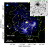 |
Fig. 12. MGCLS full-resolution (7.9″ × 7.5″; yellow) and filtered 25″ resolution (blue) Stokes-I intensity image of MCXC J0351.1−8212, showing newly detected candidate mini-halo and relic-like structures near the cluster centre. The corresponding synthesised beams are shown on the upper left. The colour scale is in square root scaling between 10−500 μJy beam−1 (yellow) and 50−800 μJy beam−1 (blue). Smoothed archival Chandra 0.5−7 keV X-ray contours (levels: 7, 12, 17, 22 × 10−8 counts cm−2 s−1) are overlaid in white. The physical scale at the cluster redshift is indicated on the lower left, and the red × marks the NED catalogue position. Inset: DSS r-band image of the dashed region in the main figure, with 15″ resolution MGCLS contours overlaid. Contours start at 3σ = 30 μJy beam−1 and increase in factors of 3. |
We note the similarity of the filamentary structures to those in Abell 133 (Slee et al. 2001; Randall et al. 2010). In that case, the filaments cap a buoyant blob of AGN material from the BCG, which has dragged up cool thermal material from the cluster core. A similar process may be at work in MCXC J0351.1−8212, although why there would be two such filamentary caps is unclear. If this is another case of buoyant lifting of the radio and X-ray plasmas, then the mini-halo-like structure may in fact be the remnant of the radio lobe(s). Deeper optical imaging and investigation of the spectral shape of the various diffuse and filamentary components may be able to distinguish between the mini-halo–relic and AGN-related scenarios.
6.2.3. J0631.3−5610: Distant AGN or faint relic?
One of the strengths of MeerKAT in the L band is its extreme sensitivity to faint extended emission. Figure 13 shows an example of one of the fainter relic-like structures detected in this survey, with the left inset panel showing the full-resolution (7.6″ × 7.5″) and filtered 25″ resolution MGCLS images in yellow and blue, respectively. The source, with a mean surface brightness of 6 μJy beam−1 in the full-resolution map, has a largest angular size of 5.9′, revealed in the filtered 25″ resolution image. The source appears to be 1.5 Mpc west of the MCXC J0631.3−5610 (z = 0.054) cluster centre, when comparing to an X-ray image of the region shown in Fig. 13. The total 1.28 GHz flux density of the radio source is 2.8 ± 0.2 mJy, measured from the filtered 25″ resolution image. At the cluster redshift and assuming a conservative spectral index of −1.0 with a 10% uncertainty, this corresponds to a k-corrected 1.4 GHz radio power of (1.7 ± 0.3) × 1022 W Hz−1.
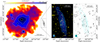 |
Fig. 13. Faint relic-like structure in the MCXC J0631.3−5610 (z = 0.054) cluster field. Left: smoothed archival XMM-Newton 0.2−12 keV count image of the cluster, with white contours at levels of 0.3, 0.5, 0.9, and 1.7 counts per pixel. The position of the relic-like source relative to the cluster region is indicated, with filtered 25″ resolution MGCLS contours of the radio source, to the west, in black; the radio source appears to be 1.5 Mpc from the cluster centre. Middle: multi-resolution MGCLS image of the radio source (yellow – 7.6″ × 7.5″ resolution; blue – filtered 25″ resolution), with cyan contours from the filtered 25″ resolution image (levels: 20, 40, 60, 80 μJy beam−1). The colour scale is in square root scaling between 8−200 μJy beam−1 (yellow) and 5−300 μJy beam−1 (blue). The physical scale at the cluster redshift is shown in the upper right corner, and the synthesised MGCLS beams in the lower left corner. Right: DSS r-band image of the same region as the middle panel. Cyan contours are the same as in the left inset, and black contours are from the 15″ resolution MGCLS image with levels of 3, 6, 10, 20 × 1σ, where σ = 10 μJy beam−1. The synthesised MGCLS beams are shown in the lower left corner. There appears to be no obvious optical counterpart for the radio source. |
The source has no obvious optical counterpart in the DSS r-band image of the region, shown in the right inset panel of Fig. 13, and no redshift information is available for any of the WISE sources in the region. Although showing no evidence of a radio core, it is possible that this source is a distant dying radio galaxy with the available optical imaging too shallow to identify a counterpart. However, given the morphology and orientation of the source relative to the X-ray emitting gas, it is possible that it is a relic or phoenix source related to the cluster. Its physical size would be ∼370 kpc at the cluster redshift. If this is a relic source, its radio power makes it the lowest luminosity relic known, a factor of 5 below the lowest luminosity relic listed by de Gasperin et al. (2014). With the low X-ray-derived cluster mass of M500 = 1.3 × 10¹⁴ M⊙ (Lovisari & Reiprich 2019), it lies just below the extrapolation of the de Gasperin et al. (2014) luminosity-mass relation. This reinforces and extends to lower masses the problem that these radio luminosities are significantly larger than those seen in simulations (e.g. Brüggen & Vazza 2020). Observational estimates of the efficiency of shock acceleration (e.g. Botteon et al. 2020) at relics also indicate improbably high values, given our current understanding.
7. Illuminating individual radio galaxies
Among the many thousands of extended radio galaxies in the survey, we highlight a small group selected for the interesting science issues they raise. The science issues include possible missing pieces of radio galaxy physics as well as complex interactions with the external medium that go beyond the simple relative motions that created tailed radio galaxies. For each source below, we indicate if it is a member of its respective target cluster; otherwise it should be considered as a serendipitous detection.
In this section we use optical overlays from the Dark Energy Camera (DECam) Legacy Survey (DECaLS), available through the Dark Energy Legacy Survey site12 and from the NOAO Astro Data Lab13, and overlays from Pan-STARRS14. An investigation of a machine learning tool to automatically identify interesting sources is discussed in Appendix C.
7.1. Lateral edge enhancement
The laterally brightened source (LBS) shown in Fig. 14 is unique in terms of the brightening of its lateral edges, along with the presence of central jet-like features of similar length and brightness in each lobe. While some radio galaxies have bright hot spot regions at their ends (defined as Fanaroff-Riley type IIs, Fanaroff & Riley 1974), brightened lateral edges are not observed. Instead, radio galaxy lateral edges are observed to either cut off sharply (e.g. when pressure-confined) or to fade slowly (see e.g. Fig. 34 in Leahy & Perley 1991). The LBS was found serendipitously in the field of cluster MCXC J2104.9−8243. Here we describe some aspects of this unique source and some possibilities (none of them very attractive) for explaining the edge brightened features.
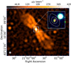 |
Fig. 14. Full-resolution (7.6″ × 7.4″) MGCLS Stokes-I intensity map of the LBS source, a unique double-lobed radio galaxy with lateral edge brightening. The inset is a DECam RGB colour composite (using the zir bands, respectively), with contours from the full-resolution MGCLS image showing the radio core centred at RA = 21h01m47.7s, Dec = −82° 09′36″ on a faint, irregularly shaped, very red object (which appears yellow-green in the zir inset). The MGCLS synthesised beam is indicated in the lower left corner. |
In most respects, the LBS appears normal. Its host is a faint, red, irregularly shaped object seen in the DECaLS image (see the inset in Fig. 14). No redshift is available. The NE and SW lobes have total MGCLS flux densities of 4.0 ± 0.8 and 1.9 ± 0.5 mJy, with lengths of 80″ and 100″, respectively. The length:width ratio of the lobes is ∼2:1. The source’s R ratio (Score/(Stotal − Score), Orr & Browne 1982) is ∼14%, within the normal range, and the core has a spectral index of ∼ − 0.9 indicating the likely presence of small-scale optically thin jets. No reliable spectral indices could be determined for the lobes.
The lobes seem to divide abruptly into three separate lengthwise narrow features (jets and edges) at an angular distance of ∼10″ from the core. Most of the flux density appears to be in these narrow features, with little indication of more extended emission. Where the jets and enhanced edges are bright, they are each somewhat resolved transversely, with deconvolved widths of ∼5−15″. Approximately half-way to the ends, the jets and bright edges all drop by a factor of ∼2 in brightness, and the structure becomes less clear.
Jets typically fade with distance from the core, as seen here, due to expansion or other energy losses. However, the fact that the transverse edges fade at the same distance from the core as the jets do is difficult to explain in current models. We briefly considered several possible explanations for this behaviour. One possibility could be that the bright edges are due to backflow from the terminus of the jet. However, this does not appear attractive because (a) no hotspots are seen, which are expected if there is strong backflow, and (b) any edge brightening due to backflows would be brighter near the end away from the host, while we observe the opposite. Another possibility is that the bright edges are regions of strong magnetic fields, perhaps generated by shear with the external medium. However, once again, there is no reason for them to drop in brightness at the same distance from the host as the jets. A hollow cylinder could perhaps be invoked for the bright edges, similar to what is seen in some bipolar nebulae (Allen & Swings 1972), but again, the correspondence with the jet profile appears fortuitous. In short, we can provide no adequate explanation for this source’s unique morphology.
7.2. Exceptionally stable bent jets
The narrow bent-tail source (NBT) shown in the top panel of Fig. 15 is unique among bent-jet sources in showing very little lateral expansion of the jets far beyond where they have bent by ∼90° from their original direction. There are many examples where no expansion may be apparent (Chibueze et al. 2021), but the resolution is insufficient to measure the widths before and after the bend. By contrast to the bent sources, straight jets can be very well-collimated, terminating in small radio and sometimes even optical hot spots subtending ≪1° as seen from the core (e.g. Roeser & Meisenheimer 1987). But bent jets such as narrow- or wide-angle tails always develop broad cocoon-like structures after the jets bend (e.g. O’Dea & Owen 1986; Rudnick & Burns 1981). As those jets bend due to their motion with respect to the surrounding medium, they tend to become unstable and are enveloped in much broader structures (O’Neill et al. 2019).
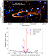 |
Fig. 15. Depiction of the NBT, showing that it remains well collimated long after it bends, a unique behaviour. Top: MGCLS Stokes-I full-resolution (7.5″ × 7.4″) intensity image in orange, overlaid on the WISE W1 image in blue. The radio brightness scale is logarithmic, saturating at 0.2 mJy beam−1. The host, centred at the south end of the twin tails, is located at RA = 07h39m23.89s, Dec = −75° 37′11.3″. The physical scale at the host redshift is indicated, and the MGCLS synthesised beam is shown in lower left corner. Bottom: increase in jet widths, in units of the jet radius near the core, as a function of distance from the core. They show the dramatic difference between the NBT and a prototypical narrow-angle tail (NGC 1265, using the 3.7″ resolution map from Gendron-Marsolais et al. 2020) and a numerically simulated tail, from O’Neill et al. (2019). |
The host of the NBT is WISE 073923.89−753711.3; at a photometric redshift of z = 0.108 (Dálya et al. 2018) it is ∼930 kpc long, placing it in the ‘giant’ class. It was found serendipitously at the very large projected distance of ∼3.7 Mpc from the nearest known cluster at a similar redshift (MCXC J0738.1−7506 at z = 0.111). The NBT’s monochromatic luminosity at 1.28 GHz is 6.4 × 10²³ W Hz−1, typical for bent-tail sources. Profiles across the eastern tail (top tail in Fig. 15) show that it broadens and fades until it disappears at ∼400 kpc from the host, while the western tail extends more than twice that.
In the bottom panel of Fig. 15 we compare the transverse expansion of the jets in NBT to those of NGC 1265, the prototypical head-tail/narrow-angle-tail galaxy (Miley 1973). We also include the results from a simulation of synchrotron radiation from a tailed radio galaxy with jets of internal Mach number M = 2.5 bent by a transverse M = 0.9 wind (O’Neill et al. 2019). The distances in each case are plotted as the straight line separation from the core, in units of the bending radius (rb) of the jets. For NBT we set rb = 35″, half the distance between the parallel tails; the apparent bending radius appears smaller near the host, but since the jets do not emerge exactly perpendicular to the direction of relative motion, they do not follow a simple circular path (see the appendix of O’Neill et al. 2019). The jet widths are measured as the FWHM for Gaussian fits to the jet/tail. In NGC 1265, the jets expand by a factor of 3 at 1.0 rb, while for the simulated jet, this occurs at ∼1.5 rb. By contrast, NBT reaches a factor of 3 expansion only at ∼10 rb.
It is not clear how to maintain this extraordinary collimation. In simulated jets, strong eddies form in the uniform surrounding medium, causing the jets to wobble and be partially disrupted (O’Neill et al. 2019). Pieces of jet thus transfer their momentum through the surrounding medium to the other tail, causing disruption events there. By this time, the extent of the synchrotron emitting region of each tail, mixed with the external medium, can be many times the initial jet width. The situation is even more complex if there are flow inhomogeneities in the surrounding medium.
It might appear attractive to invoke projection effects to make the bending radius appear smaller than it is in the true plane of the jets. However, to mimic the behaviour of the jets shown in Fig. 15, we need to assume foreshortening by a factor of ∼7, or an angle of ∼82° between the plane of the sky and the plane of the jets. At this angle, by the time the jets in NBT are moving parallel to one another, they would be separated by ∼1 Mpc. In comparison, the separation between the tails in narrow-angle tail sources (where the tails are parallel to each other), is typically of order 10s kpc (e.g. Gendron-Marsolais et al. 2020). Therefore, projected or not, NBT is unique in maintaining its collimation, and whether we are looking at a very special environment, or a new type of jet physics, remains a puzzle for the future.
7.3. A 300 kpc ring around interacting spirals
We discovered a ∼300 kpc diameter ring around two pairs of interacting spiral galaxies. To our knowledge, this structure is unique and not easily explained by currently known processes in such galaxies. In the full-resolution Stokes-I intensity image of the MACS J0417.5−1155 field, faint emission is seen in a ring-like structure around two compact radio sources ∼0.4° NW of and unrelated to the cluster. The ring becomes much more distinct in the filtered 25″ resolution intensity map, shown in Fig. 16. No other such rings are seen around stronger sources in this field or any other field in the MGCLS, so it is unlikely that the ring is an artefact.
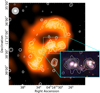 |
Fig. 16. Filtered 25″ resolution MGCLS Stokes-I intensity image of a large diffuse radio ring surrounding and connecting to an interacting pair of galaxies in the MACS J0417.5−1155 field. The brightness scale is linear and saturates at 0.2 mJy beam−1. The interacting pairs are seen in the Pan-STARRS false colour gri-composite inset. White contours show the full-resolution (7.9″ × 7.8″) MGCLS Stokes-I intensity, with a 1σ local rms noise of 6 μJy beam−1. The first two contours are at levels of 3.5 and 5σ, thereafter increasing by a factor of 3. The same contours, starting from 5σ, are shown in the inset. The synthesised beams are shown in the upper left corner (grey – filtered 25″ resolution, white – full resolution). |
Each of the bright compact radio sources near the centre overlaps a pair of interacting spiral galaxies, as shown in the Pan-STARRS gri-composite image inset in Fig. 16. The eastern radio source is centred on the brighter galaxy of its pair, WISEA J041630.96−113728.0 (also 6dFGS gJ041631.0−113728) at a redshift of 0.086 (Jones et al. 2009). The radio source is unresolved, has a flux density of 14 mJy, a spectral index of −0.76 ± 0.02, and a marginally detected ROSAT counterpart. The other galaxy in the pair, 2MASX J04163041−1137306, has a redshift of 0.087. These objects are in the foreground of the target cluster, MACS J0417.5−1155 (z = 0.44). The western radio source is also associated with the brighter member of its pair, WISEA J041628.16−113729.1, at a redshift of 0.0846, with its companion 2MASX J04162816−1137236 at a redshift of 0.083. It has a total flux density of 1.3 mJy, and a spectral index of −0.9 ± 0.05. Encircling and connecting with these compact components, the extended emission (seen in the low resolution imaging) has a total flux density of 5 ± 1 mJy and a maximum diameter of ∼300 kpc, assuming it is associated with the compact sources. The luminosity of the diffuse emission and the western compact emission are each ∼1026 W Hz−1, while the eastern source’s luminosity is an order of magnitude higher. All of these are orders of magnitude higher than expected from starburst activity (Condon 1992).
With several more galaxies, these pairs are part of the Hickson Compact Group 27 (Hickson 1982), with a diameter of 3.8′ (365 kpc), on the same scale as the radio ring. We consider first whether tidal tails could be responsible for the large ring. The tidal tails visible in the Pan-STARRS image span a smaller distance of ∼73″ (115 kpc), and the lack of distortion in the galaxies suggest that the tidal interactions are still at an early stage. Tidal tails have been observed, however, to span large distances, for example 200 kpc for the HI tails of the antennas (Hibbard et al. 2001), although synchrotron emission has only been detected out to 20 kpc (Basu et al. 2017). Whether or not tidal effects could result in star formation and subsequent cosmic-ray production, along with magnetic field amplification on the scale of the ring, is an open question.
Galaxy groups, themselves, have been found to contain both extended thermal gas and relativistic plasmas, as well as large-scale H I and cold gas (e.g. O’Sullivan et al. 2018a). In some cases, thermal gas that is too diffuse to be detected in X-rays may exist on scales all the way up to 700 kpc (Freeland & Wilcots 2011), based on the distortion of radio galaxies. Nikiel-Wroczyński et al. (2019) found diffuse emission in 17 of 20 compact groups, and Nikiel-Wroczyński et al. (2013) detected diffuse radio emission extending over about 75 kpc in Stephan’s Quintet. Group-related emission has not yet been found on the physical scale or with the luminosity, or structure, shown here. The elliptical ring of emission here is brightest on its outer edges, similar to what is seen from shocks on much larger (megaparsec) scales generated when clusters of galaxies collide (peripheral radio relics). As an alternative to a shock origin, flybys of other group galaxies could light up the remnants of previous AGN activity (e.g. O’Sullivan et al. 2018b). Determining whether shocks, AGN emission, tidal tails, or some other mechanism is responsible for this curious ring-structure in J0416−1137 will depend on deeper X-ray observations and radio spectral information.
7.4. The interaction of ICM magnetic filaments and radio tails
With MeerKAT’s exceptional combination of sensitivity and resolution, filamentary synchrotron structures are now being discovered in the neighbourhood of radio galaxies (Ramatsoku et al. 2020; Condon et al. 2021a). Here, we present the first example where a direct interaction between a filament and the jet flow from a radio galaxy may been seen. The full-resolution MGCLS image of the Abell 194 z = 0.018 cluster field is shown in Fig. 17. The newly revealed filamentary structures associated with the cluster radio galaxies 3C40A and 3C40B at the centre of Abell 194 cannot be explained with any current radio galaxy models. Such very large-scale features are not seen in numerical simulations of radio galaxies, nor were such features predicted. These sources were studied at lower resolution at multiple frequencies by Sakelliou et al. (2008) who first noted unusual extensions around the radio galaxies.
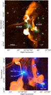 |
Fig. 17. Two radio galaxies in Abell 194, 3C40A, and 3C40B, with unusual filamentary appendages. Top: full-resolution (7.7″ × 7.5″) MGCLS Stokes-I intensity image (orange), overlaid on an Sloan Digital Sky Survey (SDSS) gri colour composite of the region (Alam et al. 2015). The radio brightness is logarithmic, saturating at 2 mJy beam−1. The physical scale at the cluster redshift of z = 0.018 is indicated in the lower left corner. Bottom: zoomed-in view of the boxed region from the top panel, with the full-resolution MGCLS image in orange on a non-monotonic scale and the SDSS r-band image in blue. The optical galaxies near the radio cores are labelled. |
The most spectacular filaments are the parallel curved pair, each ∼100″ (37 kpc) wide and extending 8.9′ (∼200 kpc) to the east from the northern lobe of NGC 547 (3C40B). The spectral index map in Fig. 18 shows that the filamentary structures have steep spectra, similar to the faintest portions of the radio galaxy lobes. Where they appear to emerge from the northern jet, the filaments curve due SE, counter to the northern jet flow.
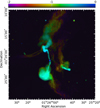 |
Fig. 18. Log intensity-coded MGCLS spectral index map of the 3C40A and 3C40B radio sources in Abell 194, at full resolution (7.7″ × 7.5″). Colours indicate the spectral index, and the brightness indicates the Stokes-I intensity. The colour bar indicates the spectral indices, with the upper (lower) part of the colour bar corresponding to the brighter (fainter) regions. The brightness is on a linear scale and saturates at 8 mJy beam−1. |
The second radio galaxy, 3C40A, is associated with NGC 541. At the higher MGCLS resolution, we can clearly see that the 165 kpc plumes observed by Sakelliou et al. (2008) are dominated by twin ∼15″ (5.5 kpc) wide filamentary structures. In addition, there is a rich network of filaments connecting to and between these two bright radio galaxies, some at lower brightness than visible in the images here. The origin of these structures is unknown.
Extensive networks of filamentary structure associated with a tailed radio galaxy are also seen in the LOw Frequency ARray maps of Abell 1314 (Fig. 25 in van Weeren et al. 2021). Ramatsoku et al. (2020) showed another spectacular example from MeerKAT observations of ESO 137−006, with ‘collimated synchrotron’ threads connecting the two radio lobes. The origin of all these features is still unknown. One speculative possibility mentioned by Parrish et al. (2012), Birkinshaw & Worrall (2015), and Donnert et al. (2018) is that there are pre-existing magnetic flux tubes in the ICM. Such features would become visible only when there was a sufficient population of relativistic electrons. Further spectral and polarisation work, and detailed comparisons with X-ray emission from the ICM will be needed to explain these novel phenomena.
7.5. A tail with ribs and tethers
At a distance of 350 kpc from the X-ray peak of Abell 3266 we identify a tailed radio galaxy (hereinafter T3266) with features not yet seen elsewhere, and whose physical origins are unclear. The structure appears in earlier maps by Bernardi et al. (2016) where it is shown to be elongated parallel to the cluster X-ray emission, positioned between the identified optical sub-clusters. The Abell 3266 galaxy cluster (listed in the MGCLS catalogue as J0431.4−6126) is likely in the midst of a complicated cluster merger, with an elongated X-ray distribution (Henriksen & Tittley 2002), two velocity-separated sub-clusters of optical galaxies in its core, and six sub-clusters on its peripheries (Dehghan et al. 2017). The cluster core has a mean redshift of 0.0594 ± 0.0005 and a velocity dispersion of 1460 ± 100 km s−1.
The full-resolution MGCLS image of T3266, overlaid on the g-band DECam image, is shown in Fig. 19. T3266 has a faint, 65 μJy beam−1 radio core (not visible in this image) associated with WISEA J043045.39−612335.6 (galaxy denoted by B in Fig. 19), at a redshift of 0.0626. The radio tail extends to the NE (from right to left in the figure), and the entire structure has a projected length of ∼6.7′ (∼480 kpc at the redshift of the presumed host). The region of the tail closest to galaxy B (the ‘ribbed tail’ in Fig. 19) shows distinct quasi-periodic changes in brightness and width. The tail is ∼20″ (23 kpc) wide at its half-intensity in this region, but its transverse profile is flat-topped and shows no signs of bifurcation. No other such features are seen in the MGCLS Abell 3266 field of view, and they are unlikely to be instrumental in origin. The four bright regions nearest the head of T3266 are separated by ∼19″ (22 kpc), essentially the same as the jet width. This suggests that some instability in the flow may be regulating this behaviour. Some faint extensions transverse to the jet are also seen.
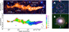 |
Fig. 19. Tailed radio source, T3266, NW of the centre of MCXC J0431.4−6126 (Abell 3266), which may be an extremely unusual composite of two independent sources. Top left: full-resolution (7.1″ × 6.7″) MGCLS Stokes-I intensity of the source (orange) overlaid on a DECam g-band image (blue). The radio brightness is on a non-monotonic scale, with the faintest regions of the tethers at ∼0.15 mJy beam−1 and the brightest regions at 2.2 mJy beam−1. Circles, labelled A and B, indicate the positions of the two likely host galaxies (see the right panels). The physical scale at the cluster redshift is shown in the lower left corner. Bottom left: in-band spectral index map, with a strong steepening with distance from host B. Right: DECam gri composite images of the two proposed hosts labelled A and B in the top left panel. Host A is at RA = 04h31m18.48s, Dec = −61° 19′18.54″. Host B is at RA = 04h30m45.56s, Dec = −61° 23′35.8″. |
Farther back along the ribbed tail, three ‘ribs’ are clearly seen to extend perpendicular to the tail axis, with a full extent of up to 75″ (88 kpc). We speculate that they reflect some type of interaction with the external medium, or are related to the transverse structures seen in early numerical simulations of intermittently restarting jets (Clarke & Burns 1991). These unusual bright patches and ribs, with their periodicity and transverse extent, stand as a challenge for the current generation of magnetohydrodynamic numerical simulations of jets in a complex ICM.
It is also possible that the full structure of T3266 may be a serendipitous projection of two separate sources, with the last 2′ of the tail (left-most in Fig. 19) potentially a separate triple source. The possible host of this source, indicated as galaxy A in Fig. 19, is a faint optical and infrared galaxy (DES J043118.45−611917.9 or WISEA J043118.50−611918.2) with a photometric redshift of 0.78 (Zou et al. 2019). If that identification is correct, the triple is a background giant radio galaxy, 900 kpc in length. The region between the ribbed tail and the triple, indicated by the dashed line in Fig. 19, and the three or more filamentary ‘tethers’, might belong to either source. They are each ∼50″ in projection, corresponding to 375 kpc and 58 kpc at the two redshifts.
It is not yet clear whether there are one or two individual radio galaxies in T3266, or even how to decisively answer that question. Either way, the tethers represent a new physical phenomenon, perhaps related to the collimated synchrotron threads of Ramatsoku et al. (2020) mentioned earlier. Unfortunately, the spectral index behaviour, seen in the bottom left panel of Fig. 19, does not provide a clear signature. In the region of the ribbed tail, T3266 shows a monotonic spectral steepening with spectral indices ranging from −0.75 at the head to −1.4 in the region of the ribs. The spectra of the tethers appear very steep (α < −2, though the spectral index is uncertain due to the low brightness of the region), and the triple source has spectral indices similar to the end of the tail, which is not expected if these are simply seen in projection.
7.6. Dying radio galaxies
One of the strengths of the MGCLS is in the detection of radio galaxies in their ‘dying phase’ (i.e. after the powering jets have been turned off). Studying such galaxies is important for understanding radio galaxy physics, the duty cycle of AGN activity, interactions with the surrounding environment, and for the usefulness of radio galaxies as cosmological probes. However, one needs a combination of high resolution (to ensure, within observational limits, that there are no significant hot spot regions or jets, and to identify the host galaxy), as well as good surface brightness sensitivity to detect the fading, dying lobes. Here we highlight two radio galaxies that might be in a dying phase of their lives, as examples of what is visible in the MGCLS data.
7.6.1. WISEA J072832.45−752740.0
The first example is shown in Fig. 20, and is associated with WISEA J072832.45−752740.0. At z = 0.0138 (Jones et al. 2009), this radio source is found serendipitously in the field of the z = 0.111 cluster MCXC J0738.1−7506. It has a total extent of ∼100 kpc, and the appearance of a wide-angle tail. Its luminosity of ∼1021 W Hz−1 is orders of magnitude below those of typical extended radio galaxies, although compact AGN emission at such low luminosities is more common (Lofthouse et al. 2018; Miller et al. 2009). The radio core, shown overlaid with a DECaLS image in the inset of Fig. 20, shows extended emission from likely interacting galaxies in a common envelope. We calculate minimum energy magnetic field strengths for each lobe, as 0.8 μG and 2 μG for the west and east lobes, respectively, assuming a spectral index of −1 and a proton/electron ratio of unity15. These imply radiative lifetimes of ∼70 Myr and ∼87 Myr, respectively, against a combination of synchrotron and Inverse Compton cooling. If the spectra were as steep as −2.5, the field strengths would increase by approximately a factor of 5, although the lifetimes would be similar, but now dominated by synchrotron losses. When the magnetic fields of dying radio galaxies drop below μG levels, the radio galaxies become very faint and the lifetimes become very short due to Inverse Compton losses (Rudnick 2004). The oldest, faintest sources will thus be rare and likely only be found in sensitive large area surveys.
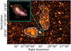 |
Fig. 20. Dying radio galaxy example, associated with WISEA J072832.45−752740.0, without detectable jets or hotspots in its diffuse lobes. The full-resolution (7.5″) MGCLS Stokes-I intensity image is shown in orange, overlaid with contours showing the filtered 25″ resolution intensity. It is outside of the primary-beam-corrected field of view of MCXC J0738.1−7506. The brightness (non-primary-beam-corrected) is on a logarithmic scale saturating at 0.1 mJy beam−1, and contours are shown at 18, 24, 34, 54, 64 μJy/(25″ beam). The inset shows a zoomed-in view of a DECaLS image of the optical host, with full-resolution radio contours, that shows recent nuclear activity. |
7.6.2. Abell 548B
In our second example, the MGCLS provides a fresh look at Abell 548B16. The MGCLS images suggest that we are dealing with a large dying radio galaxy ∼14.2′ (650 kpc) in extent. The left panel of Fig. 21 shows the diffuse emission from this source at a resolution of 25″, overlaid on a false colour gri-composite Pan-STARRS image. The radio galaxy (B) is associated with a 6dFGS source, g0545049−254740, at a redshift of 0.036, almost 2000 km s−1 from the central cluster velocity. The radio core is itself double, as seen in the top right panel where red contours are from the Very Large Array Sky Survey (VLASS) 3 GHz map at 2.5″ resolution. This structure is similar to the classes of compact symmetric objects and medium symmetric objects (Conway 2002; Augusto et al. 2006), which are thought to be young objects. This similarity may be an indication of restarting activity for the large-scale radio galaxy, but the double structure is misaligned with respect to the large lobes, so the connection is unclear.
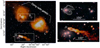 |
Fig. 21. A possible dying radio galaxy in Abell 548B. Left: diffuse emission filtered 25″ resolution MGCLS Stokes-I intensity image of Abell 548B (orange) overlaid on the false-colour gri-composite Pan-STARRS image. Previously misidentified structures (see Sect. 7.6.2 for details) are revealed to be a diffuse or dying radio galaxy to the north and a tailed radio galaxy to the south. The brightness scale is logarithmic, saturating at 1 mJy beam−1. Radio sources A–D have clear optical counterparts, with B the likely host of the diffuse lobes and A a spiral galaxy embedded in the eastern lobe. Top right: zoomed-in view of the boxed region around sources A and B. White contours, showing the 15″ resolution MGCLS Stokes-I intensity at levels of (0.3, 0.35, 0.5) mJy beam−1 and edited for clarity, indicate tailed emission associated with the spiral galaxy, A. Red compact structures are from VLASS (Lacy et al. 2020) at 3 GHz with a resolution of 2.9″ × 1.8″ (p.a. 50°). The single VLASS component associated with A has a peak flux of 30 mJy beam−1. There is a small double VLASS source associated with B, with a peak flux of 3.3 mJy beam−1, indicating possible recent radio activity. Bottom right: zoomed-in view at full resolution (7.4″ × 7.4″) of the boxed region around the tailed source, D. The brightness scale is non-monotonic, and the peak brightness in the frame is 7 mJy beam−1. 100″ corresponds to 84 kpc at the cluster redshift of 0.042. |
Embedded in the eastern lobe is a compact radio source (A) associated with the spiral galaxy 6dFGS g0545221−254730 at z = 0.038. It appears to have radio structures similar to those of a wide-angle-tail, swept towards the west by ∼80 kpc; it is not clear whether there is a physical connection to the dying radio galaxy as there is no obvious interaction with the diffuse lobe. At the western extremity, another spiral galaxy (C), likely unrelated, is seen in the radio. It is 6dFGS g0544374−255335 at z = 0.039. Finally, to the south, nearer the cluster centre, is a 220 kpc long narrow-angle tail, associated with 6dFGS g0545275−255510 (D) at z = 0.042. With their lower resolution and lower sensitivity observations, Feretti et al. (2006) suggested that the radio galaxy lobes in the north and the diffuse emission to the south were instead merger-related relic structures outside of the bright X-ray region of the cluster. Now that MGCLS has elucidated the full structure of these sources, we recognise them as a combination of diffuse-lobed and tailed radio galaxies, as described above. We expect a closer examination of the MGCLS to unveil more, and fainter, examples of dying radio galaxies.
7.7. Bulk gas motions far outside clusters
The pair of radio galaxies shown in Fig. 22 provide an unusual, and perhaps unique, case of complex radio galaxy/medium interactions far beyond the cluster environment. Early on, tailed radio galaxies provided evidence of the relative motion of their host galaxies through the ICM (Miley 1980). More recently, modest excess radio galaxy bending has also shown the influence of such motions in local overdensities at > 5 Mpc from the nearest cluster (Garon et al. 2019).
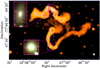 |
Fig. 22. Pair of radio galaxies with multiple bends found serendipitously in the MCXC J1840.6−7709 field, illustrating the likely effects of large-scale motions in the local external medium. The full-resolution (8.1″ × 7.6″) MGCLS Stokes-I intensity image is shown in orange, with a non-monotonic brightness scale and a peak flux of 13 mJy beam−1. A false colour zir-composite DECam image of each host is shown in the insets. The MGCLS synthesised beam is shown in the lower right corner. |
The two radio galaxies shown in Fig. 22 were found > 42′ from the centre of the z = 0.0194 cluster MCXC J1840.6−7709 (ESO 45−11). The northern source is associated with WISEA J184720.77−774444.2, at z = 0.138, and is therefore not associated with the cluster. The southern source is associated with WISEA J184722.38−774756.1, which has no available redshift; for the purposes of this discussion, we make the plausible assumption that the two radio sources belong to the same system. There are no other catalogued clusters in the vicinity, and no X-ray emission is visible in the ROSAT All-Sky Survey.
Multiple-bend sources such as these are important for understanding the dynamics of the diffuse, lower density thermal plasmas both in- and out-side of rich clusters. Simple relative motions though an external medium would produce a C-shaped structure, but the bends in these sources require other external forces. The scale sizes are of the order of several hundred kiloparsecs. In order to see bends such as these, two factors are important. First, the irregularities in the external medium flows must be on scales comparable to the size of the radio galaxy; irregularities on much smaller scales would cause small-scale structural variations that are indistinguishable from other instabilities in the jet flows, while flows on much larger scales would simply appear as relative motion, producing C-shapes. Second, the momentum flux in the external medium must be comparable to those in the jets, or they would not be perturbed. In clusters of galaxies, where similarly distorted sources are seen, thermal particle densities are of order 10−3 − 10−2 cm−3, with velocities of order 100−1000 km s−1. It is hard to see how comparable momentum fluxes could be found in the surrounding medium in such an apparently sparse environment. A more thorough examination of the environment of these galaxies would certainly be useful, as would modelling that examined the potential role of mutual orbital motions of the pair of galaxies.
8. Star-forming galaxies
Star-forming galaxies are fainter at radio frequencies than the AGN or radio galaxies presented in Sect. 7. With the depth of the MGCLS data, MeerKAT has imaged thousands of star-forming galaxies that are typically not detected in shallower all-sky surveys. Here we present some of the science possible with star-forming galaxies in the MGCLS.
8.1. Nearby spirals with MeerKAT
Radio observations of spiral galaxies provide a dust-free view of their star-forming regions, and have imaged H I beyond the optical emission boundary. Most star-forming galaxies are unresolved in the MGCLS images. However, several are resolved spirals, and here we present three examples.
8.1.1. NGC 0685 and NGC 1566
The left panel of Fig. 23 shows the 15″ resolution MGCLS view of the face-on barred spiral galaxy NGC 0685, which lies in the field of view and foreground of the MCXC J0145.0−5300 cluster. NGC 0685 (z = 0.0045) has a corrected recession velocity of 1297 km s−1 (Mould et al. 2000) and is part of the HIPASS H I (Hong et al. 2013) and Gaia DR2 (Gaia Collaboration 2018) catalogues. As expected, radio peaks are picked up in the regions of high star formation, indicated by the bluest regions in the composite DES colour image in the right panel of Fig. 23.
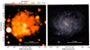 |
Fig. 23. NGC 0685, a face-on barred spiral galaxy at z = 0.0045. The physical scale is shown in the lower right corner. Left: MGCLS 15″ resolution Stokes-I intensity image, with the synthesised beam shown by the filled grey ellipse in the lower left corner. Right: DES composite gri image, with star-forming regions shown in blue. The cyan cross indicates the position of the radio peak (470 μJy beam−1), aligned with the south-west edge of the galactic bar. |
Another spectacular example of a nearby face-on spiral in the MGCLS is NGC 1566 (z = 0.0050) in the foreground of the MCXC J0416.7−5525 cluster field. This spiral galaxy is part of the IRAS Revised Bright Galaxy Sample (Sanders et al. 2003; Condon et al. 2021b) and has a Tully–Fisher-derived distance of 5.5 Mpc (Sorce et al. 2014). The full-resolution MGCLS and gri-composite DES images of this source are shown in the left and right panels of Fig. 24, respectively. This face-on Seyfert galaxy has high levels of star formation occurring in the innermost regions of the spiral arms.
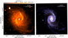 |
Fig. 24. NGC 1566, a face-on Seyfert galaxy at z = 0.0050. The physical scale is shown in the upper right corner. Left: MGCLS full-resolution (7.2″ × 7.0″) Stokes-I intensity image, with the synthesised beam shown by the filled grey ellipse in the lower left corner. Right: DES composite gri image, with star-forming regions shown in bright blue. The cyan cross indicates the position of the radio peak (31 mJy beam−1), aligned with the galactic core. |
8.1.2. An atypical star-formation ring?
A ring-like radio source, shown in the top panel of Fig. 25, is detected in the central region of the Abell 548 field. The ring, whose centre is at RA = 05h46m50.0s, Dec = −25° 38′30.4″, has a mean brightness of 45 μJy beam−1 in the full-resolution (7.5″) image, with a 130 μJy hotspot in the eastern section that has a typical AGN spectral index of −0.7. Rings in the radio sky can have several origins, including supernova remnants (Dubner & Giacani 2015), planetary nebulae (Bryce et al. 1997), star formation (Hummel et al. 1984), extreme AGN jet bending (Rawes et al. 2018), and gravitational galaxy-galaxy lensing (Hewitt et al. 1988). Ring sources with no optical counterpart, dubbed ‘odd radio circles’ (Norris et al. 2021) have also been found. They may also be attributed to Lindblad resonances (as in NGC 4736, Schommer & Sullivan 1976) or a past burst of star formation triggered by an interaction, as in the case of M 31 (Hammer et al. 2010).
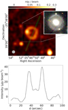 |
Fig. 25. A ring-like source in Abell 548. Top: 7.5″ resolution MGCLS Stokes-I intensity image of the ring-like source in the Abell 548 field, centred at RA = 05h46m50.0s, Dec = −25° 38′30.4″. The inset shows the Pan-STARRS gri-composite image. The ring hotspot is coincident with a background galaxy, indicated by the yellow arrow. Bottom: profile through the centre of the radio ring (green region in the top panel, with the profile starting from the northern end), showing that the structure is filled. |
The ring in Abell 548 does have an optical counterpart, as seen in the Pan-STARRS image of the region shown in the inset of Fig. 25. The counterpart is a nearby Sab-type galaxy (Thomas & Katgert 2006), WISEA J054650.08−253830.8, at z = 0.04653, which has brighter arc regions on the northern and southern edges of the spiral disc. At this redshift, the ring spans ∼33 kpc. The radio hotspot is coincident with a red background galaxy, indicated by the yellow arrow in the Pan-STARRS image in Fig. 25, and therefore unlikely to be linked to the ring itself.
The radio ring emission has a steep spectrum, with the brightest regions (for which we can obtain a reliable fit) having a spectral index of approximately −1. Such steep, non-thermal spectra are more typical of Sb and later type galaxies (Puxley et al. 1988). A slice through the centre of the ring, shown in the bottom panel of Fig. 25, indicates that there is also emission in the interior of the ring, although there is no central peak typically associated with star-forming spiral galaxies. If the ring is due to star formation, it may have been triggered by interaction with the companion galaxy (z = 0.04648) that lies 75.5″ to the north-east, outside of the region shown in Fig. 25.
8.2. Population studies in Abell 209
Galaxy clusters are populated by two broad classes of galaxies: red elliptical galaxies in which star formation has been quenched, and blue spiral galaxies with ongoing star formation (e.g. Baldry et al. 2004; Taylor et al. 2015; Haines et al. 2017). The latter types are more often found in the cluster outskirts. This leads to a relation between the fraction of star-forming galaxies and the projected distance from the cluster centre (e.g. Lewis et al. 2002; Gómez et al. 2003; Haines et al. 2015).
Here we present analyses of star-formation rates (SFRs) and the radio–far-infrared (FIR) correlation for the Abell 209 cluster field as an example of the types of population studies possible with the MGCLS. We use the optically cross-matched MGCLS compact source catalogue (see Sect. 5.2.2). Abell 209, at a redshift of z = 0.206 and with R200 = 2.15 Mpc (10.2′ on the sky), is selected due to the availability of extensive spectroscopic catalogues from the Cluster Lensing And Supernova survey with Hubble (CLASH-VLT; Annunziatella et al. 2016) and the Arizona Cluster Redshift Survey17 (ACReS; described in Haines et al. 2015) for the identification of cluster galaxies. Given MeerKAT’s large primary beam, these studies can therefore be performed out to 3.5 R200 in this cluster, unprecedented in the radio regime.
After assigning cluster membership and excising AGN (see Appendix B for details), we obtain a final catalogue of 459 MGCLS-detected star-forming cluster members within the primary-beam-corrected field of view (80 within R200)18. Figure 26 shows the fraction of star-forming cluster members that are detected by MeerKAT, fradio = NMGCLS/NoptIR (with SFR > SFR5σ), as a function of angular distance and projected distance (in units of R200 = 2.15 Mpc) from the cluster centre. Here NoptIR is the number of cluster member galaxies determined from the optical and infrared catalogues after removing AGN contamination (2476 within the field of view). We see that the fraction is lower in the cluster centre (fradio < 0.1), and rises to ∼0.2 by 2 R200. The fall in the last three radial bins is at least in part due to decreased sensitivity in the MGCLS observations due to the MeerKAT primary beam. For comparison, we show results from Haines et al. (2015) of the fraction of star-forming galaxies in a sample of 30 0.15 < z < 0.30 clusters, as measured using Herschel observations. These probe down to the same SFR limit as the MGCLS data, assume the same Chabrier (2003) initial mass function (IMF) as this work, and are not affected by dust extinction. In the region of overlap, we see a similar trend in the infrared-derived results. Haines et al. (2015) interpreted their result as evidence for relatively slow quenching of star formation in cluster galaxies over a ≈2 Gyr timescale.
 |
Fig. 26. Fraction of star-forming cluster members in Abell 209 detected in the radio (black diamonds) as a function of projected radial distance from the cluster centre, in units of R200 (bottom) and in angular units (top). We only plot MGCLS sources with SFRs greater than the 5σ detection limit of SFR5σ = 2 M⊙ yr−1 (see Appendix B for details). Grey circles show the fraction of star-forming galaxies using infrared-derived data from Haines et al. (2015) for 30 clusters. Error bars show 1σ uncertainties. A similar trend is seen out to 2 R200 for both the radio- and infrared-derived fractions. |
8.2.1. Star-formation rates
In the last few decades there have been many efforts to measure the for galaxies in a range of environments using various tracers (e.g. James et al. 2004; Elbaz et al. 2007; Karim et al. 2011, for Hα, infrared, and radio measurements, respectively). Here we use the MGCLS radio continuum luminosities to estimate SFRs for the star-forming galaxies in Abell 209 (details of the SFR determination are provided in Appendix B). The radio signal is a combination of thermal free-free (bremsstrahlung) and non-thermal synchrotron (e.g. Condon 1992). The non-thermal emission typically dominates at frequencies below 5 GHz. The 1.28 GHz MGCLS luminosities therefore provide us with dust-unbiased measurements over a ≈1 deg2 field centred on the cluster, probing radio-derived SFRs out to well beyond R200 for the first time.
Figure 27 shows the SFR of the MGCLS-detected Abell 209 star-forming member galaxies as a function of the projected distance from the cluster centre, under the assumption that the observed radio emission is due to star formation. We find no dependence of the SFR on distance from the cluster centre, based on the median SFR of the member galaxies. This is consistent with the star-formation quenching process taking place over an extended time period that is longer than the infall time (i.e. galaxies that are forming stars are not immediately quenched upon encountering the cluster environment). A similar result was found for the highest-mass star-forming galaxies in nearby clusters from the SDSS (von der Linden et al. 2010); however, the lower-mass galaxies showed more significant star-formation quenching within 0.2 R200.
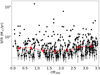 |
Fig. 27. SFR versus projected radial distance from the Abell 209 cluster centre, in units of R200, for the 429 star-forming cluster galaxies in the full primary-beam-corrected MGCLS field of view. The red triangles indicate the median SFR plotted in radial bins and show no evolution with radial distance. The dashed grey line is the SFR at the MGCLS 5σ sensitivity limit. All error bars show the 1σ uncertainty. |
8.2.2. Radio–FIR ratio
The 1.4 GHz luminosities of star-forming galaxies are tightly correlated with their luminosities (Condon 1992), with both indicating the rate of star formation. Looking at nearby galaxy clusters (z < 0.025), a small but statistically significant enhancement of the radio–FIR ratio has been found for cluster galaxies as compared to the field galaxies (Reddy & Yun 2004; Murphy et al. 2009). Gavazzi et al. (1991) suggest this enhancement could be due to the ram pressure from the interaction with the ICM, which compresses the star-forming gas and amplifies the embedded magnetic fields. Using cross-matched Herschel 100 μm flux densities for 49 Abell 209 star-forming galaxies (see Appendix B), we examined the radio–FIR correlation, looking for evidence of evolution with distance from the cluster centre.
Figure 28 shows the ratio of radio-to-FIR flux density for Abell 209 as a function of projected distance from the cluster centre in units of R200. We perform a non-linear weighted19 least-squares fit to a straight line using the log ratio versus r/R200. We obtain a best-fit relation of
 (7)
(7)
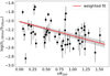 |
Fig. 28. Log ratio of radio-to-FIR flux densities for 49 star-forming cluster galaxies in Abell 209 as a function of projected radius from the cluster centre in units of R200. Black circles indicate the star-forming galaxies in the Abell 209 cluster that have MGCLS radio and Herschel FIR flux densities. All error bars are 1σ uncertainties. The red line is the weighted least-squares fit given in Eq. (7), with the grey region showing the 1σ uncertainty of the fit. |
We see a statistically significant trend for the radio–FIR ratio to increase with decreasing projected distance from the cluster centre. Our results are in line with findings from Murphy et al. (2009), who argued that this primarily arises from ram pressure stripping. The amount of ram pressure is expected to be proportional to the ICM density, but should also be dependent on cluster richness and mass. The MGCLS provides a range of clusters with which to study this further, and potentially disentangle the various effects, as well as a large enough sample of galaxies in individual clusters to look for dependences on galaxy properties.
9. HI science highlights
In conjunction with the continuum science discussed in previous sections, one of the great strengths of the MGCLS dataset is in its usefulness for mapping large volumes in H I (see Sect. 4.3.4). The sensitivity of the observations makes the MGCLS a rich resource for galaxy evolution studies that employ the H I line, especially in cases where there is ancillary data at other wavelengths available. Commensal H I science is possible not only within the clusters themselves, but also in the foreground and background as a result of the large H I volume probed by the long-track MGCLS observations. The H I data products themselves are not included in the current DR1.
H I MGCLS studies can make effective use of two low-RFI windows, between 1300−1420 MHz (0 < z < 0.09) and between 960−1190 MHz (0.19 < z < 0.48). While the first enables sampling of the H I mass function at lower redshifts, the second provides a glance into the most massive systems at higher redshift through statistical means and potentially by strong lensing of the clusters themselves. For cases where radio continuum and H I sources are spatially resolved, H I outflows (e.g. in starburst or AGN systems) can be studied, and comparisons can be made between the star formation and H I mass properties on both an individual and statistical basis. To demonstrate this, Fig. 29 shows two examples of H I discs in the MGCLS data, with very different radio continuum properties.
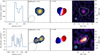 |
Fig. 29. Two demonstration examples of complementary H I and radio continuum science in the MGCLS from the Abell 3365 field. Both rows show H I discs at z ∼ 0.04 with radio continuum counterparts. Left: integrated H I spectrum with the per-channel standard deviation indicated by grey vertical bars. Centre left: total intensity H I map with the synthesised beam indicated in the lower left corner. The contour outlines the lowest level emission deemed real by the SOF IA source finding software (see Sect. 9.1.2 for details). The colour scale (from yellow to blue) shows the H I flux density from the left panel. Centre right: H I velocity map, with the colour scale (blue to red) set to the velocities for which there is non-zero flux density in the left panel. The contour is the same as in the centre left panel. Right: radio continuum intensity map, with the continuum synthesised beam indicated in the lower left corner. The colour range is between −20 and 200 μJy beam−1, and the contour is the same as in the centre left panel. |
To illustrate the H I science possible with this survey we present early results from an examination of four representative galaxy clusters, selected primarily to demonstrate data quality and potential science. The clusters, Abell 194, Abell 4038, Abell 3562, and Abell 3365, lie in the redshift range 0.01 < z < 0.1 and were selected from a heterogeneous catalogue of clusters detected in the 0.1−2.4 keV X-ray band (Piffaretti et al. 2011). They cover a reasonable range of X-ray luminosity (LX ≈ (0.07 − 1.3)×1044 erg s−1) and cluster virial mass (Mv ≈ 0.4 − 2.4 × 10¹⁴ M⊙).
9.1. H I data processing
In the following two sections we describe the methodology followed to extract H I cubes for the four cluster datasets from the MGCLS visibilities, and the procedure used to carry out H I source finding.
9.1.1. H I cubes
We created H I data cubes within the frequency interval of 1305−1430 MHz (z ≲ 0.088). The data reduction was conducted with the CARACAL20 (Józsa et al. 2020) and OXKAT21 (Heywood 2020) pipelines. The former makes use of STIMELA22, which is a radio interferometry scripting framework based on container technologies and Python (Offringa et al. 2010). Within this framework, various open-source radio interferometry software packages were used to perform all necessary procedures from cross calibration to imaging.
The final H I cubes of the four clusters cover a field of view of 1.0 deg2 each, have a median rms noise level of ∼0.1 mJy beam−1 per 44.1 km s−1 channel, and a median FWHM Gaussian restoring beam of ∼18″ (imaged with natural weighting). This noise level results in a typical 5σ H I column density sensitivity of 9 × 1019 cm−2 (0.72 M⊙ pc−2) over a line width of 44.1 km s−1.
9.1.2. H I source finding
We used the H I Source Finding Application (SOF IA, Serra et al. 2015) to search for line emission from each of the cubes. For this purpose, various tests were conducted with SOF IA noise threshold filters, smoothing kernels, and reliability parameters to ensure optimal source finding that reduced the number of false positives and ensured that the low H I surface brightness is also properly detected. We used the smooth and clip (S+C) method (Serra et al. 2012), with a noise threshold of 4 times the rms noise and spatial smoothing kernels corresponding to 1.0, 1.5, and 2.0 times the synthesised beam. Given the coarse 44.1 km s−1 velocity resolution of the MGCLS data, no smoothing was done in velocity. The catalogue of detections was compiled retaining only the positive voxels with an integrated S/N > 3.5 and reliability parameter > 0.99. This high SOF IA reliability was chosen to limit the rate of potential false detections. All detections were additionally validated by eye.
9.2. H I science examples
Here we highlight a select few of the results from this initial set of cluster analysis. As previously emphasised, these include H I detections within the clusters themselves, as well in their foregrounds and backgrounds.
9.2.1. The distribution of H I masses
Figure 30 shows the H I mass distribution of all galaxies detected in H I in clusters Abell 194 (z = 0.018), Abell 4038 (z = 0.028), and Abell 3562 (z = 0.049). The H I detection cluster membership was defined within the velocity dispersion of the clusters and the entire 1 deg2 field of view and may therefore contain interlopers. Abell 3365 (z = 0.093) is not included here as the frequencies corresponding to its redshift were heavily contaminated by RFI – a demonstration of the upper redshift limit of the 0 < z ≲ 0.09 RFI-free window.
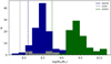 |
Fig. 30. H I mass distribution of detected galaxies in Abell 194, Abell 3562, and Abell 4038. Dashed vertical lines indicate the H I mass detection limits at the distances of each cluster, assuming a galaxy line width of 150 km s−1 detected above 4σ. |
The mass distributions in these three clusters point towards different H I populations in different clusters. The H I (redshift-dependent) mass detection limit lies below the low-mass drop in the detection rate for Abell 3562, and the lack of low-mass detections in this system is therefore not sensitivity related. By comparison, Abell 4038 shows a deficiency in high-mass H I detections. These two systems are of comparable mass (2.4 × 10¹⁴ M⊙ versus 2.0 × 10¹⁴ M⊙); however, Abell 3562 is part of the rich Shapley supercluster (Raychaudhury et al. 1991), and this environment may impact the H I mass in the system. Abell 194 is almost an order of magnitude less massive (4.0 × 10¹³ M⊙), which may account for the comparatively low number of H I galaxies detected in the system.
9.2.2. Cluster H I: Abell 194
In Fig. 31 we show the H I total intensity map of Abell 194 overlaid on an optical image. This shows the extent, richness, and some of the presumably environment-driven morphological transformation processes that influence the growth and evolution of these cluster members. By studying the full sample of appropriate clusters in the MGCLS sample, we will be able to investigate these effects on a statistical basis with a relatively uniform set of observations, as well as find rare extreme examples, given the large sample size.
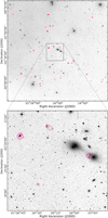 |
Fig. 31. H I detections in the Abell 194 field, with contours showing the H I column density (0.25, 1, 4 M⊙ pc−2 levels), overlaid on DSS1 optical images. The H I resolution is 19″ × 14″, p.a. 147°. Top: full cluster region showing more than 25 H I detections. Bottom: zoomed-in view of the boxed region from the top panel, showing the richness of resolved structures. Both bound H I and that in the process of being stripped from galaxies are evident. The compact H I source at RA = 01h25m47s, Dec = −01° 22′18″ is Minkowski’s object, shown also in Fig. 1D. |
9.2.3. Foreground H I: Discovery of a new H I group
The H I imaging of Abell 3365 was compromised by severe RFI at the frequency corresponding to z = 0.0926. However, this dataset showed the value of our strategy of imaging the full 0 < z ≲ 0.1 range through the serendipitous discovery of a massive H I group in the foreground of Abell 3365 at z = 0.040. This group, with a dynamical mass of Mdyn ∼ 1013 M⊙, has at least 26 members, some of which have disturbed and asymmetric H I morphologies as seen towards the centre of the group’s H I moment-0 map shown in Fig. 32.
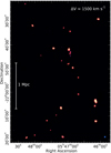 |
Fig. 32. H I moment-0 map of the newly discovered H I group at z = 0.040, which is in the foreground of the Abell 3365 cluster at z = 0.093. The colour scale has a linear stretch and is clipped outside of the range of 0 to 150 Jy beam−1 Hz. A conservative estimate is that this group has a total of 26 members within a radius of ∼2 Mpc and a velocity range of ΔV ∼ 1500 km s−1, with a mass range 8 ≲ log(MHI/M⊙)≲10. The tapered beam is shown in the lower right corner and has a dimension of 30″ × 26″. The physical scale at the group redshift is indicated. |
10. Summary and conclusions
We have presented a technical description and initial science results from the MGCLS DR1, which consists of 1.28 GHz observations of 115 radio- and X-ray-selected galaxy clusters. The full list of MGCLS targets and associated legacy product status is available in Table 1. We note that the clusters were not selected to be a homogeneous or complete sample, so care must be taken in any statistical investigation of our cluster sample as a whole.
The available DR1 products are composed of: visibilities; full field of view basic cubes without primary beam correction; primary-beam-corrected full-resolution (7−8″) and convolved (15″) Stokes-I intensity and spectral index cubes; and full-resolution primary-beam-corrected 12-frequency spectral cubes. For 40% of the clusters, full Stokes cubes suitable for Faraday rotation analysis, and limited-purpose single-plane Q and U maps, are also provided. The data products are available via the DR1 web page23 and the MGCLS website24. The website will be updated when additional data products become available.
To facilitate community usage of the MGCLS DR1 products, we produced a compact source catalogue with more than 626 000 radio sources over the 115 cluster fields (Sect. 5.2), as well as optical and infrared DECaLS cross-match catalogues for the compact sources in the Abell 209 and Abell S295 fields (Sect. 5.2.2). We have also provided a list of 59 multi-component extended radio sources in these two cluster fields (Sect. 5.3). Finally, in Table 4 we have provided a catalogue of diffuse cluster radio emission, containing 99 distinct sources detected in 62 of the MGCLS fields, 56 of which are new.
We have also presented some early science results using the DR1 data, with some significant science findings, and have highlighted the potential for future community study. In particular, we reported:
-
The lowest luminosity radio relic candidate detected to date (Sect. 6.2.3) by exploiting the excellent surface brightness sensitivity of the MGCLS.
-
Diffuse structures in several clusters that do not fall cleanly into the typical classes of mini-halo, halo, or relic, indicating the need for new dynamical, particle acceleration, or field amplification processes in the ICM (Sect. 6 and Table 4).
-
Radio galaxy structures that cannot be explained using current models (Sect. 7), including trident-like structures, jets that stay well collimated far past their bending radius, and filamentary features connecting, at least in projection, with otherwise normal radio galaxy structures.
-
The detection of 459 star-forming galaxies out to ∼3.5 R200 in Abell 209 (Sect. 8.2). We find no SFR evolution with distance from the cluster centre, and a reduction in the ratio of radio to 100 μm flux densities with increased cluster-centric distance.
-
Early results from H I studies of four MGCLS clusters (Sect. 9), including H I mass distributions in three clusters, and a new foreground H I group in the Abell 3365 field.
The results presented here represent only a small fraction of what can be achieved with the DR1 legacy dataset. Follow-up projects by the MGCLS team and the broader community are likely to make significant contributions to many areas of astrophysics.
Operated by the South African Radio Astronomy Observatory (SARAO).
The NASA/IPAC Extragalactic Database is operated by the Jet Propulsion Laboratory, California Institute of Technology, under contract with the National Aeronautics and Space Administration.
These standard sets of calibration tables are not part of the MGCLS but can be provided upon reasonable request.
When using DR1 products, this paper should be cited, and the MeerKAT telescope acknowledgement included. See https://doi.org/10.48479/7epd-w356 for details.
Available at https://doi.org/10.48479/7epd-w356
Statistical uncertainties on the in-band spectral index are less than 0.05 in these regions.
The source is at the edge of where we can make reliable primary beam corrections, and the S/N is low enough that the fluxes could be uncertain by up to ∼50%. This leads to an uncertainty of ∼12% in the derived fields, which is much lower than the uncertainties from the other assumptions.
Abell 548B is the western component of what was originally classified as Abell 548, as described in Dressler & Shectman (1988).
This catalogue forms the basis of a value-added catalogue for Abell 209 being provided with the MGCLS DR1, which includes radio-derived SFRs for each galaxy and the ratio of radio-to-FIR flux densities (where available). See Appendix B for details of these additional measurements and Table B.1 for an excerpt of the catalogue.
Weights are the 1σ uncertainties in the log ratio.
For galaxies that have both a spectroscopic and photometric redshift, inclusion as a cluster member is defined by the spectroscopic redshift.
The PACS Point Source Catalogue from the NASA/IPAC Infrared Science Archive: https://irsa.ipac.caltech.edu/cgi-bin/Gator/nph-scan?submit=Selectprojshort=HERSCHEL
Available at https://michellelochner.github.io/mgcls.astronomaly
Acknowledgments
The MeerKAT telescope is operated by the South African Radio Astronomy Observatory, which is a facility of the National Research Foundation, an agency of the Department of Science and Innovation. The authors acknowledge the contribution of those who designed and built the MeerKAT instrument. The authors thank the anonymous reviewer for their helpful comments which improved the manuscript. KK and ML acknowledge funding support from the South African Radio Astronomy Observatory (SARAO) and the National Research Foundation (NRF). WDC acknowledges support from the National Radio Astronomy Observatory, which is a facility of the National Science Foundation operated by Associated Universities, Inc. Partial support for LR comes from US National Science Foundation grant AST17-14205 to the University of Minnesota. Basic research in radio astronomy at the US Naval Research Laboratory for TEC is supported by 6.1 Base Funding. RPD, SR, and GL’s research is funded by the South African Research Chairs Initiative of the DSI/NRF (grant ID: 77948). MR’s research is supported by the SARAO HCD programme via the “New Scientific Frontiers with Precision Radio Interferometry” research group grant. VP acknowledges financial support from the South African Research Chairs Initiative of the Department of Science and Innovation and NRF. Opinions expressed and conclusions arrived at are those of the authors and are not necessarily to be attributed to the NRF. TV acknowledges the support from the Ministero degli Affari Esteri della Cooperazione Internazionale – Direzione Generale per la Promozione del Sistema Paese Progetto di Grande Rilevanza ZA18GR02. We thank E. Egami for providing access to ACReS data. Some results published here have made use of the CARACAL pipeline, partially supported by ERC Starting grant number 679629 ‘FORNAX’, MAECI Grant Number ZA18GR02, DST-NRF Grant Number 113121 as part of the ISARP Joint Research Scheme, and BMBF project 05A17PC2 for D-MeerKAT. We acknowledge the use of computing facilities of the Inter-University Institute for Data Intensive Astronomy (IDIA) for part of this work. IDIA is a partnership of the Universities of Cape Town, of the Western Cape, and of Pretoria. This research made use of Astropy (http://www.astropy.org), a community-developed core Python package for Astronomy, and routines from the publicly available Astromatch package authored by A. Ruiz. It also made use of the SAOImageDS9 (Joye et al. 2003) software for image preparation, and the NASA/IPAC Extragalactic Database (NED) and NASA/IPAC Infrared Science Archive (IRSA), which are funded by the National Aeronautics and Space Administration and operated by the California Institute of Technology. Chandra X-ray Observatory data shown in this paper were accessed through the Chandra Data Archive (ObsIDs: 13380, 15173, 16283). XMM-Newton data shown in this paper were accessed through the XMM-Newton Science Archive (ObsID: 0720253401). The Digitized Sky Surveys were produced at the Space Telescope Science Institute under US Government grant NAG W-2166. The images of these surveys are based on photographic data obtained using the Oschin Schmidt Telescope on Palomar Mountain and the UK Schmidt Telescope. The plates were processed into the present compressed digital form with the permission of these institutions. DECam data were obtained through the Legacy Surveys imaging of the DESI footprint, which is supported by the Director, Office of Science, Office of High Energy Physics of the US Department of Energy under Contract No. DE-AC02-05CH1123, by the National Energy Research Scientific Computing Center, a DOE Office of Science User Facility under the same contract; and by the US National Science Foundation, Division of Astronomical Sciences under Contract No. AST-0950945 to NOAO. DECam data were also obtained from the Astro Data Lab at NSF’s National Optical-Infrared Astronomy Research Laboratory. NOIRLab is operated by the Association of Universities for Research in Astronomy (AURA), Inc. under a cooperative agreement with the National Science Foundation. The Pan-STARRS1 Surveys (PS1) and the PS1 public science archive have been made possible through contributions by the Institute for Astronomy, the University of Hawaii, the Pan-STARRS Project Office, the Max-Planck Society and its participating institutes, the Max Planck Institute for Astronomy, Heidelberg and the Max Planck Institute for Extraterrestrial Physics, Garching, the Johns Hopkins University, Durham University, the University of Edinburgh, the Queen’s University Belfast, the Harvard-Smithsonian Center for Astrophysics, the Las Cumbres Observatory Global Telescope Network Incorporated, the National Central University of Taiwan, the Space Telescope Science Institute, the National Aeronautics and Space Administration under Grant No. NNX08AR22G issued through the Planetary Science Division of the NASA Science Mission Directorate, the National Science Foundation Grant No. AST-1238877, the University of Maryland, Eotvos Lorand University (ELTE), the Los Alamos National Laboratory, and the Gordon and Betty Moore Foundation. The Very Large Array Sky Survey (VLASS) is a project of the National Radio Astronomy Observatory, which is a facility of the US National Science Foundation operated under cooperative agreement by Associated Universities, Inc.
References
- Alam, S., Albareti, F. D., Allende Prieto, C., et al. 2015, ApJS, 219, 12 [Google Scholar]
- Allen, D. A., & Swings, J. P. 1972, ApJ, 174, 583 [NASA ADS] [CrossRef] [Google Scholar]
- Annunziatella, M., Mercurio, A., Biviano, A., et al. 2016, A&A, 585, A160 [NASA ADS] [CrossRef] [EDP Sciences] [Google Scholar]
- Assef, R. J., Stern, D., Kochanek, C. S., et al. 2013, ApJ, 772, 26 [Google Scholar]
- Assef, R. J., Stern, D., Noirot, G., et al. 2018, ApJS, 234, 23 [Google Scholar]
- Augusto, P., Gonzalez-Serrano, J. I., Perez-Fournon, I., & Wilkinson, P. N. 2006, MNRAS, 368, 1411 [CrossRef] [Google Scholar]
- Bacchi, M., Feretti, L., Giovannini, G., & Govoni, F. 2003, A&A, 400, 465 [NASA ADS] [CrossRef] [EDP Sciences] [Google Scholar]
- Bagchi, J., Durret, F., Neto, G. B. L., & Paul, S. 2006, Science, 314, 791 [NASA ADS] [CrossRef] [Google Scholar]
- Baldry, I. K., Glazebrook, K., Brinkmann, J., et al. 2004, ApJ, 600, 681 [Google Scholar]
- Banda-Barragán, W. E., Federrath, C., Crocker, R. M., & Bicknell, G. V. 2018, MNRAS, 473, 3454 [CrossRef] [Google Scholar]
- Basu, A., Mao, S. A., Kepley, A. A., et al. 2017, MNRAS, 464, 1003 [NASA ADS] [CrossRef] [Google Scholar]
- Beers, T. C., Flynn, K., & Gebhardt, K. 1990, AJ, 100, 32 [Google Scholar]
- Bell, E. F. 2003, ApJ, 586, 794 [Google Scholar]
- Bernardi, G., Venturi, T., Cassano, R., et al. 2016, MNRAS, 456, 1259 [NASA ADS] [CrossRef] [Google Scholar]
- Birkinshaw, M., & Worrall, D. 2015, IAU Gen. Assem., 29, 2258369 [Google Scholar]
- Blanton, E. L., Gregg, M. D., Helfand, D. J., Becker, R. H., & White, R. L. 2003, AJ, 125, 1635 [CrossRef] [Google Scholar]
- Bock, D. C. J., Large, M. I., & Sadler, E. M. 1999, AJ, 117, 1578 [Google Scholar]
- Bonafede, A., Brüggen, M., van Weeren, R., et al. 2012, MNRAS, 426, 40 [Google Scholar]
- Bonafede, A., Intema, H. T., Bruggen, M., et al. 2014, MNRAS, 444, L44 [Google Scholar]
- Bonafede, A., Cassano, R., Brüggen, M., et al. 2017, MNRAS, 470, 3465 [Google Scholar]
- Botteon, A., Gastaldello, F., Brunetti, G., & Kale, R. 2016, MNRAS, 463, 1534 [Google Scholar]
- Botteon, A., Brunetti, G., Ryu, D., & Roh, S. 2020, A&A, 634, A64 [NASA ADS] [CrossRef] [EDP Sciences] [Google Scholar]
- Brown, S., & Rudnick, L. 2011, MNRAS, 412, 2 [Google Scholar]
- Brüggen, M., & Vazza, F. 2020, MNRAS, 493, 2306 [Google Scholar]
- Brüggen, M., Reiprich, T. H., Bulbul, E., et al. 2021, A&A, 647, A3 [NASA ADS] [CrossRef] [EDP Sciences] [Google Scholar]
- Brunetti, G., & Jones, T. W. 2014, Int. J. Mod. Phys. D, 23, 1430007 [Google Scholar]
- Brunetti, G., Setti, G., Feretti, L., & Giovannini, G. 2001, MNRAS, 320, 365 [Google Scholar]
- Brunetti, G., Giacintucci, S., Cassano, R., et al. 2008, Nature, 455, 944 [Google Scholar]
- Bryce, M., Pedlar, A., Muxlow, T., Thomasson, P., & Mellema, G. 1997, MNRAS, 284, 815 [NASA ADS] [CrossRef] [Google Scholar]
- Camilo, F., Scholz, P., Serylak, M., et al. 2018, ApJ, 856, 180 [Google Scholar]
- Cassano, R., Ettori, S., Giacintucci, S., et al. 2010, ApJ, 721, L82 [Google Scholar]
- Cassano, R., Ettori, S., Brunetti, G., et al. 2013, ApJ, 777, 141 [Google Scholar]
- Chabrier, G. 2003, PASP, 115, 763 [Google Scholar]
- Charlot, P., Jacobs, C. S., Gordon, D., et al. 2020, A&A, 644, A159 [EDP Sciences] [Google Scholar]
- Chibueze, J. O., Sakemi, H., Ohmura, T., et al. 2021, Nature, 593, 47 [NASA ADS] [CrossRef] [Google Scholar]
- Churazov, E., Khabibullin, I., Lyskova, N., Sunyaev, R., & Bykov, A. M. 2021, A&A, 651, A41 [NASA ADS] [CrossRef] [EDP Sciences] [Google Scholar]
- Clarke, D. A., & Burns, J. O. 1991, ApJ, 369, 308 [NASA ADS] [CrossRef] [Google Scholar]
- Colafrancesco, S., Mhlahlo, N., Jarrett, T., Oozeer, N., & Marchegiani, P. 2016, MNRAS, 456, 512 [NASA ADS] [CrossRef] [Google Scholar]
- Condon, J. J. 1992, ARA&A, 30, 575 [Google Scholar]
- Condon, J. J. 1997, PASP, 109, 166 [NASA ADS] [CrossRef] [Google Scholar]
- Condon, J. J., Cotton, W. D., Greisen, E. W., et al. 1998, AJ, 115, 1693 [Google Scholar]
- Condon, J. J., Cotton, W. D., White, S. V., et al. 2021a, ApJ, 917, 18 [CrossRef] [Google Scholar]
- Condon, J. J., Cotton, W. D., Jarrett, T., et al. 2021b, ApJS, 257, 35 [NASA ADS] [CrossRef] [Google Scholar]
- Conway, J. E. 2002, New Astron. Rev., 46, 263 [CrossRef] [Google Scholar]
- Cotton, W. D. 2008, PASP, 120, 439 [Google Scholar]
- Cotton, W. D. 2019, Obit Development Memo Series, 63, 1, ftp://ftp.cv.nrao.edu/NRAO-staff/bcotton/Obit/MFImage.pdf [Google Scholar]
- Cotton, W. D., Condon, J. J., Kellermann, K. I., et al. 2018, ApJ, 856, 67 [Google Scholar]
- Cowie, L. L., & McKee, C. F. 1975, A&A, 43, 337 [NASA ADS] [Google Scholar]
- Cuciti, V., Cassano, R., Brunetti, G., et al. 2021a, A&A, 647, A51 [EDP Sciences] [Google Scholar]
- Cuciti, V., Cassano, R., Brunetti, G., et al. 2021b, A&A, 647, A50 [NASA ADS] [CrossRef] [EDP Sciences] [Google Scholar]
- Dallacasa, D., Brunetti, G., Giacintucci, S., et al. 2009, ApJ, 699, 1288 [NASA ADS] [CrossRef] [Google Scholar]
- Dálya, G., Galgóczi, G., Dobos, L., et al. 2018, MNRAS, 479, 2374 [Google Scholar]
- de Gasperin, F., van Weeren, R. J., Brüggen, M., et al. 2014, MNRAS, 444, 3130 [NASA ADS] [CrossRef] [Google Scholar]
- de Gasperin, F., Intema, H. T., Shimwell, T. W., et al. 2017, Sci. Adv., 3, e1701634 [Google Scholar]
- Dehghan, S., Johnston-Hollitt, M., Colless, M., & Miller, R. 2017, MNRAS, 468, 2645 [NASA ADS] [CrossRef] [Google Scholar]
- de Villiers, M. S., Venter, M., & Peens-Hough, A. 2021, IEEE Trans. Antennas Propag., 69, 6333 [CrossRef] [Google Scholar]
- Dey, A., Schlegel, D. J., Lang, D., et al. 2019, AJ, 157, 168 [Google Scholar]
- Di Gennaro, G., van Weeren, R. J., Hoeft, M., et al. 2018a, ApJ, 865, 24 [Google Scholar]
- Di Gennaro, G., Venturi, T., Dallacasa, D., et al. 2018b, A&A, 620, A25 [NASA ADS] [CrossRef] [EDP Sciences] [Google Scholar]
- Di Gennaro, G., van Weeren, R. J., Brunetti, G., et al. 2021, Nat. Astron., 5, 268 [Google Scholar]
- Donnert, J., Vazza, F., Brüggen, M., & ZuHone, J. 2018, Space Sci. Rev., 214, 122 [Google Scholar]
- Dressler, A., & Shectman, S. A. 1988, AJ, 95, 985 [Google Scholar]
- Dubner, G., & Giacani, E. 2015, A&ARv, 23, 3 [Google Scholar]
- Duchesne, S. W., Johnston-Hollitt, M., Offringa, A. R., et al. 2021a, PASA, 38, e010 [NASA ADS] [CrossRef] [Google Scholar]
- Duchesne, S. W., Johnston-Hollitt, M., & Bartalucci, I. 2021b, PASA, 38, e053 [CrossRef] [Google Scholar]
- Duchesne, S. W., Johnston-Hollitt, M., & Wilber, A. G. 2021c, PASA, 38, e031 [NASA ADS] [CrossRef] [Google Scholar]
- Dwarakanath, K. S., Malu, S., & Kale, R. 2011, JApA, 32, 529 [Google Scholar]
- Dwarakanath, K. S., Parekh, V., Kale, R., & George, L. T. 2018, MNRAS, 477, 957 [NASA ADS] [CrossRef] [Google Scholar]
- Ebeling, H., Edge, A. C., & Henry, J. P. 2001, ApJ, 553, 668 [Google Scholar]
- Elbaz, D., Daddi, E., Le Borgne, D., et al. 2007, A&A, 468, 33 [NASA ADS] [CrossRef] [EDP Sciences] [Google Scholar]
- Ensslin, T. A., Biermann, P. L., Klein, U., & Kohle, S. 1998, A&A, 332, 395 [NASA ADS] [Google Scholar]
- Enßlin, T. A., & Brüggen, M. 2002, MNRAS, 331, 1011 [Google Scholar]
- Fanaroff, B. L., & Riley, J. M. 1974, MNRAS, 167, 31P [Google Scholar]
- Feretti, L., Schuecker, P., Böhringer, H., Govoni, F., & Giovannini, G. 2005, A&A, 444, 157 [NASA ADS] [CrossRef] [EDP Sciences] [Google Scholar]
- Feretti, L., Bacchi, M., Slee, O. B., et al. 2006, MNRAS, 368, 544 [NASA ADS] [CrossRef] [Google Scholar]
- Feretti, L., Giovannini, G., Govoni, F., & Murgia, M. 2012, A&ARv, 20, 54 [Google Scholar]
- Ferrari, C., Arnaud, M., Ettori, S., Maurogordato, S., & Rho, J. 2006, A&A, 446, 417 [NASA ADS] [CrossRef] [EDP Sciences] [Google Scholar]
- Finoguenov, A., Sarazin, C. L., Nakazawa, K., Wik, D. R., & Clarke, T. E. 2010, ApJ, 715, 1143 [Google Scholar]
- Flesch, E. W. 2019, ArXiv e-prints [arXiv:1912.05614] [Google Scholar]
- Freeland, E., & Wilcots, E. 2011, ApJ, 738, 145 [NASA ADS] [CrossRef] [Google Scholar]
- Gaia Collaboration 2018, VizieR Online Data Catalog: I/345 [Google Scholar]
- Garon, A. F., Rudnick, L., Wong, O. I., et al. 2019, AJ, 157, 126 [Google Scholar]
- Gavazzi, G., Boselli, A., & Kennicutt, R. 1991, AJ, 101, 1207 [NASA ADS] [CrossRef] [Google Scholar]
- Gendron-Marsolais, M., Hlavacek-Larrondo, J., van Weeren, R. J., et al. 2020, MNRAS, 499, 5791 [NASA ADS] [CrossRef] [Google Scholar]
- George, L. T., Dwarakanath, K. S., Johnston-Hollitt, M., et al. 2015, MNRAS, 451, 4207 [Google Scholar]
- George, L. T., Dwarakanath, K. S., Johnston-Hollitt, M., et al. 2017, MNRAS, 467, 936 [Google Scholar]
- Giacintucci, S., Venturi, T., Brunetti, G., et al. 2005, A&A, 440, 867 [NASA ADS] [CrossRef] [EDP Sciences] [Google Scholar]
- Giacintucci, S., Venturi, T., Macario, G., et al. 2008, A&A, 486, 347 [NASA ADS] [CrossRef] [EDP Sciences] [Google Scholar]
- Giacintucci, S., Markevitch, M., Cassano, R., et al. 2017, ApJ, 841, 71 [Google Scholar]
- Giovannini, G., & Feretti, L. 2000, New Astron., 5, 335 [Google Scholar]
- Giovannini, G., Feretti, L., & Stanghellini, C. 1991, A&A, 252, 528 [NASA ADS] [Google Scholar]
- Giovannini, G., Tordi, M., & Feretti, L. 1999, New Astron., 4, 141 [CrossRef] [Google Scholar]
- Giovannini, G., Feretti, L., Govoni, F., Murgia, M., & Pizzo, R. 2006, Astron. Nachr., 327, 563 [Google Scholar]
- Giovannini, G., Bonafede, A., Feretti, L., et al. 2009, A&A, 507, 1257 [NASA ADS] [CrossRef] [EDP Sciences] [Google Scholar]
- Golovich, N., Dawson, W. A., Wittman, D. M., et al. 2019, ApJ, 882, 69 [NASA ADS] [CrossRef] [Google Scholar]
- Gómez, P. L., Nichol, R. C., Miller, C. J., et al. 2003, ApJ, 584, 210 [Google Scholar]
- Govoni, F., Feretti, L., Giovannini, G., et al. 2001, A&A, 376, 803 [NASA ADS] [CrossRef] [EDP Sciences] [Google Scholar]
- Gunn, J. E., & Gott, J. R., III 1972, ApJ, 176, 1 [Google Scholar]
- Haines, C. P., Pereira, M. J., Smith, G. P., et al. 2015, ApJ, 806, 101 [NASA ADS] [CrossRef] [Google Scholar]
- Haines, C. P., Iovino, A., Krywult, J., et al. 2017, A&A, 605, A4 [NASA ADS] [CrossRef] [EDP Sciences] [Google Scholar]
- Hammer, F., Yang, Y. B., Wang, J. L., et al. 2010, ApJ, 725, 542 [NASA ADS] [CrossRef] [Google Scholar]
- Helou, G., Madore, B. F., Schmitz, M., et al. 1991, in The NASA/IPAC Extragalactic Database, eds. M. A. Albrecht, & D. Egret, 171, 89 [NASA ADS] [Google Scholar]
- Henriksen, M. J., & Tittley, E. R. 2002, ApJ, 577, 701 [NASA ADS] [CrossRef] [Google Scholar]
- Hewitt, J. N., Turner, E. L., Schneider, D. P., Burke, B. F., & Langston, G. I. 1988, Nature, 333, 537 [NASA ADS] [CrossRef] [Google Scholar]
- Heywood, I. 2020, Astrophysics Source Code Library [record ascl:2009.003] [Google Scholar]
- Hibbard, J. E., van der Hulst, J. M., Barnes, J. E., & Rich, R. M. 2001, AJ, 122, 2969 [NASA ADS] [CrossRef] [Google Scholar]
- Hickson, P. 1982, ApJ, 255, 382 [NASA ADS] [CrossRef] [Google Scholar]
- Hilton, M., Sifón, C., Naess, S., et al. 2021, ApJS, 253, 3 [Google Scholar]
- Hindson, L., Johnston-Hollitt, M., Hurley-Walker, N., et al. 2014, MNRAS, 445, 330 [NASA ADS] [CrossRef] [Google Scholar]
- Hong, T., Staveley-Smith, L., Masters, K. L., et al. 2013, MNRAS, 432, 1178 [NASA ADS] [CrossRef] [Google Scholar]
- Hummel, E., van der Hulst, J. M., & Dickey, J. M. 1984, A&A, 134, 207 [NASA ADS] [Google Scholar]
- HyeongHan, K., Jee, M. J., Rudnick, L., et al. 2020, ApJ, 900, 127 [NASA ADS] [CrossRef] [Google Scholar]
- Intema, H. T., Jagannathan, P., Mooley, K. P., & Frail, D. A. 2017, A&A, 598, A78 [NASA ADS] [CrossRef] [EDP Sciences] [Google Scholar]
- James, P. A., Shane, N. S., Beckman, J. E., et al. 2004, A&A, 414, 23 [NASA ADS] [CrossRef] [EDP Sciences] [Google Scholar]
- Johnston-Hollitt, M. 2003, PhD Thesis, University of Adelaide, Australia [Google Scholar]
- Jonas, J., & MeerKAT Team 2016, MeerKAT Science: On the Pathway to the SKA, 1 [Google Scholar]
- Jones, D. H., Read, M. A., Saunders, W., et al. 2009, MNRAS, 399, 683 [Google Scholar]
- Jones, M. G., Haynes, M. P., Giovanelli, R., & Moorman, C. 2018, MNRAS, 477, 2 [Google Scholar]
- Joye, W. A., & Mandel, E. 2003, in Astronomical Data Analysis Software and Systems XII, eds. H. E. Payne, R. I. Jedrzejewski, & R. N. Hook, ASP Conf. Ser., 295, 489 [NASA ADS] [Google Scholar]
- Józsa, G. I. G., White, S. V., Thorat, K., et al. 2020, in ADASS XXIX, eds. R. Pizzo, E. Deul, J. D. Mol, J. de Plaa, & H. Verkouter, ASP Conf. Ser., 527, 635 [Google Scholar]
- Kale, R., Dwarakanath, K. S., Bagchi, J., & Paul, S. 2012, MNRAS, 426, 1204 [NASA ADS] [CrossRef] [Google Scholar]
- Kale, R., Venturi, T., Giacintucci, S., et al. 2015, A&A, 579, A92 [NASA ADS] [CrossRef] [EDP Sciences] [Google Scholar]
- Kale, R., Wik, D. R., Giacintucci, S., et al. 2017, MNRAS, 472, 940 [NASA ADS] [CrossRef] [Google Scholar]
- Kale, R., Shende, K. M., & Parekh, V. 2019, MNRAS, 486, L80 [NASA ADS] [CrossRef] [Google Scholar]
- Kang, H. 2017, J. Korean Astron. Soc., 50, 93 [NASA ADS] [CrossRef] [Google Scholar]
- Karim, A., Schinnerer, E., Martínez-Sansigre, A., et al. 2011, ApJ, 730, 61 [Google Scholar]
- Knowles, K., Pillay, D. S., Amodeo, S., et al. 2021, MNRAS, 504, 1749 [NASA ADS] [CrossRef] [Google Scholar]
- Kuźmicz, A., Jamrozy, M., Bronarska, K., Janda-Boczar, K., & Saikia, D. J. 2018, ApJS, 238, 9 [Google Scholar]
- Lacy, M., Baum, S. A., Chandler, C. J., et al. 2020, PASP, 132, 035001 [Google Scholar]
- Laird, E. S., Nandra, K., Georgakakis, A., et al. 2009, ApJS, 180, 102 [NASA ADS] [CrossRef] [Google Scholar]
- Leahy, J. P., & Perley, R. A. 1991, AJ, 102, 537 [Google Scholar]
- Lelli, F., Fraternali, F., & Verheijen, M. 2014, A&A, 563, A27 [NASA ADS] [CrossRef] [EDP Sciences] [Google Scholar]
- Lewis, I., Balogh, M., De Propris, R., et al. 2002, MNRAS, 334, 673 [NASA ADS] [CrossRef] [Google Scholar]
- Liang, H., Hunstead, R. W., Birkinshaw, M., & Andreani, P. 2000, ApJ, 544, 686 [Google Scholar]
- Lindner, R. R., Baker, A. J., Hughes, J. P., et al. 2014, ApJ, 786, 49 [NASA ADS] [CrossRef] [Google Scholar]
- Lochner, M., & Bassett, B. A. 2021, Astron. Comput., 36, 100481 [NASA ADS] [CrossRef] [Google Scholar]
- Lofthouse, E. K., Kaviraj, S., Smith, D. J. B., & Hardcastle, M. J. 2018, MNRAS, 479, 807 [Google Scholar]
- Loi, F., Murgia, M., Govoni, F., et al. 2017, MNRAS, 472, 3605 [NASA ADS] [CrossRef] [Google Scholar]
- Lovisari, L., & Reiprich, T. H. 2019, MNRAS, 483, 540 [Google Scholar]
- Luchsinger, K. M., Lacy, M., Jones, K. M., et al. 2015, AJ, 150, 87 [CrossRef] [Google Scholar]
- Macario, G., Venturi, T., Intema, H. T., et al. 2013, A&A, 551, A141 [NASA ADS] [CrossRef] [EDP Sciences] [Google Scholar]
- Macario, G., Intema, H. T., Ferrari, C., et al. 2014, A&A, 565, A13 [NASA ADS] [CrossRef] [EDP Sciences] [Google Scholar]
- Mancuso, C., Lapi, A., Prandoni, I., et al. 2017, ApJ, 842, 95 [Google Scholar]
- Mauch, T., Murphy, T., Buttery, H. J., et al. 2003, MNRAS, 342, 1117 [Google Scholar]
- Mauch, T., Cotton, W., Condon, J., et al. 2020, ApJ, 888, 61 [NASA ADS] [CrossRef] [Google Scholar]
- Mazzotta, P., & Giacintucci, S. 2008, ApJ, 675, L9 [Google Scholar]
- Mhlahlo, N., & Jamrozy, M. 2021, MNRAS, 508, 2910 [NASA ADS] [CrossRef] [Google Scholar]
- Miley, G. K. 1973, A&A, 26, 413 [NASA ADS] [Google Scholar]
- Miley, G. 1980, ARA&A, 18, 165 [Google Scholar]
- Miley, G. K., Perola, G. C., van der Kruit, P. C., & van der Laan, H. 1972, Nature, 237, 269 [NASA ADS] [CrossRef] [Google Scholar]
- Miller, N. A., Hornschemeier, A. E., Mobasher, B., et al. 2009, AJ, 137, 4450 [NASA ADS] [CrossRef] [Google Scholar]
- Mohan, N., & Rafferty, D. 2015, Astrophysics Source Code Library [record ascl:1502.007] [Google Scholar]
- Mould, J. R., Huchra, J. P., Freedman, W. L., et al. 2000, ApJ, 529, 786 [Google Scholar]
- Murphy, E. J., Kenney, J. D. P., Helou, G., Chung, A., & Howell, J. H. 2009, ApJ, 694, 1435 [CrossRef] [Google Scholar]
- Nakamura, M., & Asada, K. 2013, ApJ, 775, 118 [NASA ADS] [CrossRef] [Google Scholar]
- Nikiel-Wroczyński, B., Soida, M., Urbanik, M., Beck, R., & Bomans, D. J. 2013, MNRAS, 435, 149 [CrossRef] [Google Scholar]
- Nikiel-Wroczyński, B., Berger, A., Herrera Ruiz, N., et al. 2019, A&A, 622, A23 [EDP Sciences] [Google Scholar]
- Norris, R. P., Intema, H. T., Kapińska, A. D., et al. 2021, PASA, 38, e003 [NASA ADS] [CrossRef] [Google Scholar]
- Ochsenbein, F., Bauer, P., & Marcout, J. 2000, A&AS, 143, 23 [NASA ADS] [CrossRef] [EDP Sciences] [Google Scholar]
- O’Dea, C. P., & Owen, F. N. 1986, ApJ, 301, 841 [CrossRef] [Google Scholar]
- Offringa, A. R., de Bruyn, A. G., Biehl, M., et al. 2010, MNRAS, 405, 155 [NASA ADS] [Google Scholar]
- O’Neill, B. J., Jones, T. W., Nolting, C., & Mendygral, P. J. 2019, ApJ, 884, 12 [CrossRef] [Google Scholar]
- Orr, M. J. L., & Browne, I. W. A. 1982, MNRAS, 200, 1067 [CrossRef] [Google Scholar]
- Orrù, E., Murgia, M., Feretti, L., et al. 2007, A&A, 467, 943 [NASA ADS] [CrossRef] [EDP Sciences] [Google Scholar]
- O’Sullivan, E., Combes, F., Salomé, P., et al. 2018a, A&A, 618, A126 [NASA ADS] [CrossRef] [EDP Sciences] [Google Scholar]
- O’Sullivan, E., Kolokythas, K., Kantharia, N. G., et al. 2018b, MNRAS, 473, 5248 [CrossRef] [Google Scholar]
- Ozawa, T., Nakanishi, H., Akahori, T., et al. 2015, PASJ, 67, 110 [NASA ADS] [CrossRef] [Google Scholar]
- Parekh, V., Dwarakanath, K. S., Kale, R., & Intema, H. 2017, MNRAS, 464, 2752 [NASA ADS] [CrossRef] [Google Scholar]
- Parrish, I. J., McCourt, M., Quataert, E., & Sharma, P. 2012, MNRAS, 422, 704 [NASA ADS] [CrossRef] [Google Scholar]
- Pearce, C. J. J., van Weeren, R. J., Andrade-Santos, F., et al. 2017, ApJ, 845, 81 [Google Scholar]
- Perley, R. A., & Butler, B. J. 2013, ApJS, 206, 16 [Google Scholar]
- Piffaretti, R., Arnaud, M., Pratt, G. W., Pointecouteau, E., & Melin, J. B. 2011, A&A, 534, A109 [NASA ADS] [CrossRef] [EDP Sciences] [Google Scholar]
- Plavin, A., Cotton, W. D., & Mauch, T. 2020, Obit Development Memo Series, 62, 1, ftp://ftp.cv.nrao.edu/NRAO-staff/bcotton/Obit/MKPoln.pdf [Google Scholar]
- Puxley, P. J., Hawarden, T. G., & Mountain, C. M. 1988, MNRAS, 231, 465 [NASA ADS] [CrossRef] [Google Scholar]
- Ramatsoku, M., Murgia, M., Vacca, V., et al. 2020, A&A, 636, L1 [NASA ADS] [CrossRef] [EDP Sciences] [Google Scholar]
- Randall, S. W., Clarke, T. E., Nulsen, P. E. J., et al. 2010, ApJ, 722, 825 [NASA ADS] [CrossRef] [Google Scholar]
- Rawes, J., Birkinshaw, M., & Worrall, D. M. 2018, MNRAS, 480, 3644 [NASA ADS] [CrossRef] [Google Scholar]
- Raychaudhury, S., Fabian, A. C., Edge, A. C., Jones, C., & Forman, W. 1991, MNRAS, 248, 101 [NASA ADS] [Google Scholar]
- Reddy, N. A., & Yun, M. S. 2004, ApJ, 600, 695 [NASA ADS] [CrossRef] [Google Scholar]
- Reid, R. I., Kronberg, P. P., & Perley, R. A. 1999, ApJS, 124, 285 [NASA ADS] [CrossRef] [Google Scholar]
- Reynolds, J. E. 1994, A Revised Flux Scale for the AT Compact Array, ATNF Memo, AT/39.3/040 [Google Scholar]
- Richard-Laferrière, A., Hlavacek-Larrondo, J., Nemmen, R. S., et al. 2020, MNRAS, 499, 2934 [Google Scholar]
- Roeser, H.-J., & Meisenheimer, K. 1987, ApJ, 314, 70 [CrossRef] [Google Scholar]
- Rottgering, H. J. A., Wieringa, M. H., Hunstead, R. W., & Ekers, R. D. 1997, MNRAS, 290, 577 [Google Scholar]
- Rudnick, L. 2002, PASP, 114, 427 [Google Scholar]
- Rudnick, L. 2004, J. Korean Astron. Soc., 37, 329 [NASA ADS] [CrossRef] [Google Scholar]
- Rudnick, L., & Burns, J. O. 1981, ApJ, 246, L69 [NASA ADS] [CrossRef] [Google Scholar]
- Sakelliou, I., Hardcastle, M. J., & Jetha, N. N. 2008, MNRAS, 384, 87 [CrossRef] [Google Scholar]
- Sanders, D. B., Mazzarella, J. M., Kim, D. C., Surace, J. A., & Soifer, B. T. 2003, AJ, 126, 1607 [Google Scholar]
- Sandhu, P., Malu, S., Raja, R., & Datta, A. 2018, Ap&SS, 363, 133 [NASA ADS] [CrossRef] [Google Scholar]
- Schommer, R. A., & Sullivan, W. T., III 1976, Astrophys. Lett., 17, 191 [NASA ADS] [Google Scholar]
- Serra, P., Oosterloo, T., Morganti, R., et al. 2012, MNRAS, 422, 1835 [Google Scholar]
- Serra, P., Westmeier, T., Giese, N., et al. 2015, MNRAS, 448, 1922 [Google Scholar]
- Shakouri, S., Johnston-Hollitt, M., & Pratt, G. W. 2016, MNRAS, 459, 2525 [Google Scholar]
- Shimwell, T. W., Brown, S., Feain, I. J., et al. 2014, MNRAS, 440, 2901 [Google Scholar]
- Shimwell, T. W., Markevitch, M., Brown, S., et al. 2015, MNRAS, 449, 1486 [Google Scholar]
- Shimwell, T. W., Luckin, J., Brüggen, M., et al. 2016, MNRAS, 459, 277 [Google Scholar]
- Simpson, C., Martínez-Sansigre, A., Rawlings, S., et al. 2006, MNRAS, 372, 741 [NASA ADS] [CrossRef] [Google Scholar]
- Slee, O. B., & Reynolds, J. E. 1984, PASA, 5, 516 [NASA ADS] [CrossRef] [Google Scholar]
- Slee, O. B., Roy, A. L., & Savage, A. 1994, Aust. J. Phys., 47, 145 [CrossRef] [Google Scholar]
- Slee, O. B., Roy, A. L., Murgia, M., Andernach, H., & Ehle, M. 2001, AJ, 122, 1172 [NASA ADS] [CrossRef] [Google Scholar]
- Smith, D. J. B., Dunne, L., Maddox, S. J., et al. 2011, MNRAS, 416, 857 [Google Scholar]
- Smolčić, V., Novak, M., Bondi, M., et al. 2017, A&A, 602, A1 [Google Scholar]
- Sommer, M. W., Basu, K., Intema, H., et al. 2017, MNRAS, 466, 996 [Google Scholar]
- Sorce, J. G., Tully, R. B., Courtois, H. M., et al. 2014, MNRAS, 444, 527 [Google Scholar]
- Stern, D., Assef, R. J., Benford, D. J., et al. 2012, ApJ, 753, 30 [Google Scholar]
- Stuardi, C., Bonafede, A., Wittor, D., et al. 2019, MNRAS, 489, 3905 [NASA ADS] [Google Scholar]
- Sunyaev, R. A., & Zeldovich, Y. B. 1972, Comments Astrophys. Space Phys., 4, 173 [NASA ADS] [EDP Sciences] [Google Scholar]
- Sutherland, W., & Saunders, W. 1992, MNRAS, 259, 413 [Google Scholar]
- Taylor, E. N., Hopkins, A. M., Baldry, I. K., et al. 2015, MNRAS, 446, 2144 [NASA ADS] [CrossRef] [Google Scholar]
- Thomas, T., & Katgert, P. 2006, A&A, 446, 19 [NASA ADS] [CrossRef] [EDP Sciences] [Google Scholar]
- Turner, J. S., & Taylor, G. I. 1957, Proc. R. Soc. London Ser. A: Math. Phys. Sci., 239, 61 [NASA ADS] [Google Scholar]
- van Weeren, R. J., Röttgering, H. J. A., Brüggen, M., & Hoeft, M. 2010, Science, 330, 347 [Google Scholar]
- van Weeren, R. J., Brüggen, M., Röttgering, H. J. A., & Hoeft, M. 2011a, JApA, 32, 505 [NASA ADS] [Google Scholar]
- van Weeren, R. J., Brüggen, M., Röttgering, H. J. A., et al. 2011b, A&A, 533, A35 [NASA ADS] [CrossRef] [EDP Sciences] [Google Scholar]
- van Weeren, R. J., Bonafede, A., Ebeling, H., et al. 2012, MNRAS, 425, L36 [NASA ADS] [CrossRef] [Google Scholar]
- van Weeren, R. J., Andrade-Santos, F., Dawson, W. A., et al. 2017, Nat. Astron., 1, 0005 [Google Scholar]
- van Weeren, R. J., de Gasperin, F., Akamatsu, H., et al. 2019, Space Sci. Rev., 215, 16 [Google Scholar]
- van Weeren, R. J., Shimwell, T. W., Botteon, A., et al. 2021, A&A, 651, A115 [NASA ADS] [CrossRef] [EDP Sciences] [Google Scholar]
- Venturi, T., Bardelli, S., Morganti, R., & Hunstead, R. W. 2000, MNRAS, 314, 594 [NASA ADS] [CrossRef] [Google Scholar]
- Venturi, T., Bardelli, S., Dallacasa, D., et al. 2003, A&A, 402, 913 [NASA ADS] [CrossRef] [EDP Sciences] [Google Scholar]
- Venturi, T., Giacintucci, S., Brunetti, G., et al. 2007, A&A, 463, 937 [NASA ADS] [CrossRef] [EDP Sciences] [Google Scholar]
- Venturi, T., Giacintucci, S., Dallacasa, D., et al. 2013, A&A, 551, A24 [NASA ADS] [CrossRef] [EDP Sciences] [Google Scholar]
- von der Linden, A., Wild, V., Kauffmann, G., White, S. D. M., & Weinmann, S. 2010, MNRAS, 404, 1231 [Google Scholar]
- Walker, R. C., Hardee, P. E., Davies, F. B., Ly, C., & Junor, W. 2018, ApJ, 855, 128 [Google Scholar]
- Wilber, A. G., Johnston-Hollitt, M., Duchesne, S. W., et al. 2020, PASA, 37, e040 [NASA ADS] [CrossRef] [Google Scholar]
- Wright, E. L., Eisenhardt, P. R. M., Mainzer, A. K., et al. 2010, AJ, 140, 1868 [Google Scholar]
- Xie, C., van Weeren, R. J., Lovisari, L., et al. 2020, A&A, 636, A3 [NASA ADS] [CrossRef] [EDP Sciences] [Google Scholar]
- Yu, H., Diaferio, A., Agulli, I., Aguerri, J. A. L., & Tozzi, P. 2016, ApJ, 831, 156 [CrossRef] [Google Scholar]
- Zhang, C., Churazov, E., Dolag, K., Forman, W. R., & Zhuravleva, I. 2020, MNRAS, 494, 4539 [NASA ADS] [CrossRef] [Google Scholar]
- Zou, H., Gao, J., Zhou, X., & Kong, X. 2019, ApJS, 242, 8 [Google Scholar]
- ZuHone, J. A., Markevitch, M., & Lee, D. 2011, ApJ, 743, 16 [Google Scholar]
- ZuHone, J. A., Markevitch, M., Brunetti, G., & Giacintucci, S. 2013, ApJ, 762, 78 [Google Scholar]
Appendix A: Extended source catalogues
Here we present the extended, multi-component source catalogues for the Abell 209 (Table A.1) and Abell S295 (Table A.2) cluster fields. (See the discussion in Sect. 5.3).
Extended sources in the Abell 209 MGCLS field.
Extended sources in the Abell S295 MGCLS field.
Appendix B: Star-forming galaxy catalogue for Abell 209: SFR and radio–FIR
To carry out the environment-dependent studies discussed in Sect. 8.2, namely galaxy SFRs and the radio-FIR correlation in Abell 209, we needed to identify which of the MGCLS-detected sources belong to the cluster, remove AGN-dominated sources from that group, and calculate the SFR and the radio-FIR ratio. Here we discuss the details of these procedures and the creation of the Abell 209 star-forming galaxies catalogue being released as part of the DR1 products. This catalogue includes the SFRs and radio–FIR ratios for the cluster’s star-forming galaxies used in the scientific analyses presented in Sect. 8.2. An excerpt of this catalogue is shown in Table B.1.
Excerpt of the SFR and infrared catalogue of star-forming cluster galaxies in Abell 209, used in the SFR and radio–FIR studies in this paper (Sects. 8.2.1 and 8.2.2, respectively). The full catalogue is available online.
B.1. Cluster galaxy membership
We assigned cluster membership using a combination of spectroscopic, zs, and photometric, zp, redshifts, with the latter determined using the zCluster photometric redshift code (Hilton et al. 2021) and photometry from DECaLS (Dey et al. 2019). The CLASH-VLT (Annunziatella et al. 2016) and ACReS (Haines et al. 2015) spectroscopic datasets contain secure redshifts for 1256 and 345 galaxies in the Abell 209 field, respectively, with a combined total of 1425 unique galaxies. We define spectroscopic cluster member galaxies as those with peculiar radial velocities within ±3 σv of the cluster redshift,
where σv = 1320 km s−1 is the line of sight velocity dispersion (Annunziatella et al. 2016). Photometry-based cluster membership is defined as those galaxies with |zp − zc|< 3 σbw(1 + zc), where zc is the cluster redshift of 0.206 and σbw = 0.03 is the scatter in our photometric redshift residuals. This scatter is determined using a bi-weight scale estimate (Beers et al. 1990), and the residuals are calculated as Δz/(1 + zs), where Δz = zs − zp.
We obtained a final catalogue of 523 MGCLS-detected cluster members within the primary-beam-corrected field of view, with 98 members within R200. We determine the amount of contamination in the photometric redshift sample using the 91 member galaxies with both spectroscopic and photometric redshifts25. We find that 16% of the members selected using photometric redshifts have spectroscopic redshifts outside the photometric redshift cut range, while 23% of the spectroscopically identified cluster galaxies are missed by the photometric redshift selection.
B.2. AGN contamination
To separate star-forming galaxies from AGN-dominated galaxies, we used the ‘R90’ WISE infrared-selection criteria by Assef et al. (2018) (see also Stern et al. 2012; Assef et al. 2013). These utilise only the WISE W1−W2 colour to identify AGN without a threshold that depends on the W2 band magnitude (see Eq. (4) of Assef et al. 2018, which identifies AGN with 90% reliability). With this selection method, we classify 64 radio-detected cluster galaxies as AGN and remove them from the cluster member sample. This leaves a total of 459 MGCLS-detected star-forming cluster members within the primary-beam-corrected field of view (80 within R200). Table B.1 presents an excerpt of the catalogue of star-forming cluster galaxies in Abell 209.
B.2. Radio-derived star-formation rates
To estimate the SFR from the radio luminosities we used the Bell (2003) relation (see also Karim et al. 2011) scaled to a Chabrier (2003) IMF:
 (B.1)
(B.1)
Here, L = L1.4 GHz is the radio luminosity in W Hz−1 derived from the MGCLS 1.28 GHz total flux density, using a power law scaling and assuming a non-thermal spectral index of −0.8 (Condon 1992). Lc = 6.4 × 10²¹ W Hz−1 is taken to be the typical radio luminosity of an L* galaxy. Bell (2003) argued that galaxies with low luminosities could have their non-thermal emission significantly suppressed and therefore need to be separated from the population with higherpg luminosities. However, as only a small percentage (39/459) of the final sample have luminosities lower than Lc, we do notpg separate according to luminosity. We measure SFRs ranging between 1.2 and 432 M⊙ yr−1, within the range of knownpg values. Under the assumption that the radio emission is due to star formation, the median 5σ sensitivity limit corresponds topg
SFR5σ > 2 M⊙ yr−1, with 429/459 star-forming members with SFRs above this limit.
B.3. FIR cross-matching for radio–FIR correlation
In order to study the radio–FIR correlation in Abell 209, we first need to determine FIR flux densities for the cluster star-formingpg galaxies. We cross-match the catalogue of 459 star-forming members with the Herschel 100 μm catalogue26. This yielded 49 star-forming cluster galaxies with both 1.28 GHzpg and 100 μm flux densities. We use the log of the ratio of these two quantities to investigate evolution in the radio–FIR relation.pg
The Herschel 100 μm flux densities for the 49 galaxies and associated radio–FIR ratio are provided in the Abell 209pg star-forming galaxies catalogue shown in Table B.1.
Appendix C: Automated searches for interesting objects
The definition of an ‘unusual’ radio object is subjective and dependent on the science case of interest. In the search for radio galaxies of interest, several of which are presented in Sect. 7, the MGCLS dataset was small enough for human inspection. However, it took a significant amount of time, with all images inspected by several people and the final set of radio galaxies of interest determined after cross-checking the various choices. For future surveys, exhaustive human searches for unusual objects may be impossible. We therefore used the MGCLS to examine the efficacy of machine learning techniques to find atypical, interesting objects.
ASTRONOMALY (Lochner & Bassett 2021) is a machine learning framework designed to automatically detect anomalous (rare or unusual) objects in very large datasets. We ran ASTRONOMALY on 128 px × 128 px (160″ × 160″) cutouts around components from the PYBDSF source finding (see Sect. 5), using the same framework as Lochner & Bassett (2021). To compare our results with those from human inspection, we restricted our search to the cluster fields where we had visually identified at least one extended radio galaxy with complex and/or unusual morphology (approximately 40% of the full sample). For those fields, we centred cutouts on components that were classified as having two or more Gaussian components by PYBDSF, which resulted in 21,449 cutouts.
We used ASTRONOMALY’s anomaly score to order the data from most to least anomalous, comparing this list with a selected set of 43 sources that were previously identified as ‘interesting’ by one or more team members. Cutouts of the top 10 scoring objects are presented in Fig. C.1. Of the 43 interesting objects, ASTRONOMALY detected 22 in the top 1% (210 objects) of the rankings. Forty out of 43 sources are found in the first 10% of the list, while the remaining three could not be distinguished from ‘normal’ sources. We note that the vast majority of the 210 most highly ranked sources27 are actually visually quite similar to the selected 43. We conclude that ASTRONOMALY can be a useful tool for rapid searches of morphologically interesting objects in large catalogues of radio sources, from which more targeted manual searches can be made efficiently.
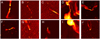 |
Fig. C.1. Ten top-ranked cutouts based on their ASTRONOMALY score. The cutouts are each 160″ per side, and their respective cluster fields (and cutout centres, in degrees of R.A., Dec.) are as follows: A: J0216.3−4816 (34.190, −47.836); B: J1423.7−5412 (214.984, −54.102); C: Abell 22 (5.055, −24.925); D: Abell 194 (21.502, −1.345); E: Abell S295 (41.422, −52.962); F: J0607.0−4928 (92.267, −48.900); G: Pandora (4.279, −29.934); H: J0216.3−4816 (33.252, −47.690); I: Abell 194 (21.522, −1.446); and J: J0738.1−7506 (114.851, −75.618). We note that sources D (and its extension to the south, identified as a separate source, I) and J are among the individual sources identified manually (independent of ASTRONOMALY) and selected for discussion in Sect. 7. |
All Tables
Excerpt of the compact source catalogue for Abell 209 with optical cross-match information from DECaLS.
Excerpt of the SFR and infrared catalogue of star-forming cluster galaxies in Abell 209, used in the SFR and radio–FIR studies in this paper (Sects. 8.2.1 and 8.2.2, respectively). The full catalogue is available online.
All Figures
|
Fig. 1. Capabilities of the MGCLS data. Panel A: brightness cutouts from the MCXC J0027.3−5015 field, showing MeerKAT’s instantaneous sensitivity to a range of angular scales. From left to right: full-resolution (7.4″ × 7.0″), convolved 25″ resolution, and filtered ‘diffuse emission’ at 25″ resolution. The synthesised beam is shown in grey in the lower left corner of each image. The colour scale is in square root scaling in each case, with a minimum and maximum brightness of −10 and 600 μJy beam−1 (left), 6 and 400 μJy beam−1 (middle), and 25 and 150 μJy beam−1 (right), respectively. See Sect. 4.3.1 for further details. Panel B: example of an in-band spectral index map of a bent tailed source in the MCXC J0431.4−6126 field, with total intensity coloured by spectral index. The host galaxy, 2MASX J04302197−6132001, is coincident with the radio core (seen in cyan). The colour scale indicates the spectral index, and the brightness gradient of the colour bar indicates intensity, with a burned-out maximum of 10 mJy beam−1. Regions where the S/N was too low to determine a spectral index have been left white. The synthesised beam (7.1″ × 6.7″) is shown by the grey ellipse in the lower left corner. Panel C: example of an RM map of a complex MGCLS source in the Abell 3667 field. Contours are Stokes-I intensity with levels of (5, 10, 20, 40, 60, 80, 100) × σ, where σ = 6.7 μJy beam−1. To avoid including spurious RM values, pixels with Stokes-I intensity below 8σ have been masked. Panel D: H I velocity map of Minkowski’s object in Abell 194, at a resolution of 19″ × 15″ (beam shown at the top left). Contours show the integrated H I flux density at levels of (0.35, 0.7, 1.4, 2.5) mJy beam−1. Colours indicate the relative velocity from −22 km s−1 (blue) to +22 km s−1 (red) from the central velocity of 5553 km s−1. |
| In the text | |
|
Fig. 2. H I mass sensitivity for the MGCLS. Top: logarithm of the total H I mass sensitivity as a function of redshift for integration times between 3 h and 12 h (not all MGCLS datasets have the same usable on-source time for H I analysis). The shaded areas indicate the H I mass limits of the MGCLS data assuming a 5σ detection for a galaxy with line width ranging from 44 km s−1 to 300 km s−1. Bottom: column-density sensitivity versus angular resolution at z = 0.03 for different integration times present in the MGCLS. The horizontal axis scale is proportional to HPBW−2. |
| In the text | |
|
Fig. 3. Comparison between the integrated flux density of MGCLS compact sources with their counterparts in the NVSS (top) and SUMSS (bottom) catalogues, with the latter two being scaled to the MGCLS frequency of 1.28 GHz. The best-fit relation in each case is shown by the solid red line and is consistent with a linear relationship, with the number of sources in the fit shown in the upper left corner. The dashed grey line shows the exact one-to-one relationship. The scaled sky survey flux densities are typically 6% higher than their MGCLS counterparts, so this represents a possible small bias in the MGCLS flux scale. Histograms show the relevant flux density distributions, with the dashed black lines indicating the respective median values, |
| In the text | |
|
Fig. 4. Spectral index distributions for the cross-matched MGCLS compact sources, using data from the MGCLS (1.28 GHz), NVSS (1.4 GHz), SUMSS (843 MHz), and TGSS (148 MHz) catalogues. Left to right: distributions for MGCLS sources with flux density measurements at two, three, and four frequencies, respectively. The number of compact sources, Ns, and the median spectral index, |
| In the text | |
|
Fig. 5. Histograms of the RA and Dec angular separations between the positions of radio sources in the Abell 209 compact source catalogue and their optical counterparts, for LR > 0.5. In each panel, the red line shows the normalised Gaussian distribution. |
| In the text | |
|
Fig. 6. Completeness (left axis, solid lines) and purity (right axis, dashed lines) versus the LR for Abell 209 (black) and Abell S295 (red). Imposing a LR cutoff at 0.5 (vertical dotted line) for Abell 209, the estimated spurious identification rate (error rate, or 1 – purity) is 4.5%, with a completeness of 59%. |
| In the text | |
|
Fig. 7. Full-resolution (7.6″ × 7.4″) MGCLS Stokes-I intensity image of a multi-host structure in the field of Abell 209. We indicate the two possible intersecting multi-component radio galaxies (giant radio galaxy and a distorted tailed galaxy). The compact radio components circled in green indicate the positions of the likely optical hosts, while the magenta circles indicate other superposed or nearby compact radio emission with optical counterparts. The brightness scale is logarithmic and saturates at 1 mJy beam−1. The synthesised beam is indicated in the lower right corner. |
| In the text | |
|
Fig. 8. Multi-resolution MGCLS view of Abell 85. Top: full-resolution (7.7″ × 7.1″; yellow, log scale between 0.006 and 2 mJy beam−1) and filtered 25″ resolution (blue, log scale between 0.06 and 3 mJy beam−1) Stokes-I intensity image of Abell 85, with the bright BCG and tailed radio galaxy emission filtered out. Smoothed archival Chandra 0.5−7 keV X-ray contours (levels: 1.0, 1.7, 3.4, 6.8, 13.6 × 10⁻⁷ counts cm−2 s−1) are overlaid in white. The respective synthesised MGCLS beams are shown on the lower left. The physical scale at the cluster redshift is indicated on the upper left, and the red × marks the NED cluster position. A newly detected elongated mini-halo (largest linear size ∼370 kpc) is seen around the cluster BCG. Filamentary structures are seen in the known phoenix/revived fossil plasma source SW of the cluster. Bottom: Pan-STARRS r-band images of the boxed regions from the top panel, with MGCLS 15″ resolution contours overlaid. Contour levels start at 3σ = 30 μJy beam−1 and increase by factors of 3. |
| In the text | |
|
Fig. 9. MGCLS full-resolution (8.6″; yellow) and diffuse emission filtered 25″ resolution (blue) Stokes-I intensity image of a portion of the RXC J0520.7−1328 field, showing complex extended emission within the region. The corresponding synthesised beams are shown on the lower left by the filled yellow and blue ellipses, respectively. The colour scales are in square root scaling between 10−500 μJy beam−1 (yellow) and 20−500 μJy beam−1 (blue). The physical scale at the cluster redshift is indicated on the lower right, and the cross marks the NED cluster position. Smoothed archival Chandra 0.5−7 keV X-ray contours (levels: 3, 6, 12, 24 × 10−8 counts cm−2 s−1) are overlaid in white, with RXC J0520.7−1328 and its companion cluster 1WGA J0521.0−1333 labelled. Dashed green ellipses indicate the regions of diffuse emission, D1 to D4, identified in Macario et al. (2014). The full-resolution MGCLS image contains artefacts that radiate from the bright compact source in RXC J0520.7−1328. |
| In the text | |
|
Fig. 10. Inferred magnetic field angles for the north-west relic in Abell 3667, after correction for Faraday rotation (which is shown in Fig. 1). Blue contours show the full-resolution (7.5″ × 7.4″) Stokes-I MGCLS intensity, with the synthesised beam shown in the boxed region on the lower left. Contour levels are 10, 20, 40, 60, 80, 100 × 1σ, where σ = 6.7 μJy beam−1. Magnetic field vectors (angles only) are shown where the linearly polarised intensity is > 8σ. The magnetic field is highly ordered along the NW edge of the relic. |
| In the text | |
|
Fig. 11. MGCLS view of the newly detected multiple-relic and radio halo system in MCXC J0352.4−7401. Top: MGCLS full-resolution (7.0″ × 6.8″; yellow) and filtered 25″ resolution (blue) Stokes-I intensity images. The colour scales are in square root scaling between 50−500 μJy beam−1 (yellow) and 5−300 μJy beam−1 (blue). Synthesised MGCLS beams are shown on the lower right, and the physical scale at the cluster redshift is shown on the upper left. The red × marks the NED cluster position, and the black cross indicates the position of a 3 mJy compact source coincident with the SE relic. Smoothed archival Chandra 0.5−7 keV contours (levels: 4, 8, 16, 30 × 10−7 counts cm−2 s−1) are overlaid in white. Bottom: in-band spectral index (left) and spectral index uncertainty (right) maps of the dashed region from the top panel, with 15″ resolution MGCLS intensity contours overlaid. Contours start at 5σ = 40 μJy beam−1 and increase in factors of 4. The synthesised beam is indicated by the filled grey circle on the lower right of each panel. |
| In the text | |
|
Fig. 12. MGCLS full-resolution (7.9″ × 7.5″; yellow) and filtered 25″ resolution (blue) Stokes-I intensity image of MCXC J0351.1−8212, showing newly detected candidate mini-halo and relic-like structures near the cluster centre. The corresponding synthesised beams are shown on the upper left. The colour scale is in square root scaling between 10−500 μJy beam−1 (yellow) and 50−800 μJy beam−1 (blue). Smoothed archival Chandra 0.5−7 keV X-ray contours (levels: 7, 12, 17, 22 × 10−8 counts cm−2 s−1) are overlaid in white. The physical scale at the cluster redshift is indicated on the lower left, and the red × marks the NED catalogue position. Inset: DSS r-band image of the dashed region in the main figure, with 15″ resolution MGCLS contours overlaid. Contours start at 3σ = 30 μJy beam−1 and increase in factors of 3. |
| In the text | |
|
Fig. 13. Faint relic-like structure in the MCXC J0631.3−5610 (z = 0.054) cluster field. Left: smoothed archival XMM-Newton 0.2−12 keV count image of the cluster, with white contours at levels of 0.3, 0.5, 0.9, and 1.7 counts per pixel. The position of the relic-like source relative to the cluster region is indicated, with filtered 25″ resolution MGCLS contours of the radio source, to the west, in black; the radio source appears to be 1.5 Mpc from the cluster centre. Middle: multi-resolution MGCLS image of the radio source (yellow – 7.6″ × 7.5″ resolution; blue – filtered 25″ resolution), with cyan contours from the filtered 25″ resolution image (levels: 20, 40, 60, 80 μJy beam−1). The colour scale is in square root scaling between 8−200 μJy beam−1 (yellow) and 5−300 μJy beam−1 (blue). The physical scale at the cluster redshift is shown in the upper right corner, and the synthesised MGCLS beams in the lower left corner. Right: DSS r-band image of the same region as the middle panel. Cyan contours are the same as in the left inset, and black contours are from the 15″ resolution MGCLS image with levels of 3, 6, 10, 20 × 1σ, where σ = 10 μJy beam−1. The synthesised MGCLS beams are shown in the lower left corner. There appears to be no obvious optical counterpart for the radio source. |
| In the text | |
|
Fig. 14. Full-resolution (7.6″ × 7.4″) MGCLS Stokes-I intensity map of the LBS source, a unique double-lobed radio galaxy with lateral edge brightening. The inset is a DECam RGB colour composite (using the zir bands, respectively), with contours from the full-resolution MGCLS image showing the radio core centred at RA = 21h01m47.7s, Dec = −82° 09′36″ on a faint, irregularly shaped, very red object (which appears yellow-green in the zir inset). The MGCLS synthesised beam is indicated in the lower left corner. |
| In the text | |
|
Fig. 15. Depiction of the NBT, showing that it remains well collimated long after it bends, a unique behaviour. Top: MGCLS Stokes-I full-resolution (7.5″ × 7.4″) intensity image in orange, overlaid on the WISE W1 image in blue. The radio brightness scale is logarithmic, saturating at 0.2 mJy beam−1. The host, centred at the south end of the twin tails, is located at RA = 07h39m23.89s, Dec = −75° 37′11.3″. The physical scale at the host redshift is indicated, and the MGCLS synthesised beam is shown in lower left corner. Bottom: increase in jet widths, in units of the jet radius near the core, as a function of distance from the core. They show the dramatic difference between the NBT and a prototypical narrow-angle tail (NGC 1265, using the 3.7″ resolution map from Gendron-Marsolais et al. 2020) and a numerically simulated tail, from O’Neill et al. (2019). |
| In the text | |
|
Fig. 16. Filtered 25″ resolution MGCLS Stokes-I intensity image of a large diffuse radio ring surrounding and connecting to an interacting pair of galaxies in the MACS J0417.5−1155 field. The brightness scale is linear and saturates at 0.2 mJy beam−1. The interacting pairs are seen in the Pan-STARRS false colour gri-composite inset. White contours show the full-resolution (7.9″ × 7.8″) MGCLS Stokes-I intensity, with a 1σ local rms noise of 6 μJy beam−1. The first two contours are at levels of 3.5 and 5σ, thereafter increasing by a factor of 3. The same contours, starting from 5σ, are shown in the inset. The synthesised beams are shown in the upper left corner (grey – filtered 25″ resolution, white – full resolution). |
| In the text | |
|
Fig. 17. Two radio galaxies in Abell 194, 3C40A, and 3C40B, with unusual filamentary appendages. Top: full-resolution (7.7″ × 7.5″) MGCLS Stokes-I intensity image (orange), overlaid on an Sloan Digital Sky Survey (SDSS) gri colour composite of the region (Alam et al. 2015). The radio brightness is logarithmic, saturating at 2 mJy beam−1. The physical scale at the cluster redshift of z = 0.018 is indicated in the lower left corner. Bottom: zoomed-in view of the boxed region from the top panel, with the full-resolution MGCLS image in orange on a non-monotonic scale and the SDSS r-band image in blue. The optical galaxies near the radio cores are labelled. |
| In the text | |
|
Fig. 18. Log intensity-coded MGCLS spectral index map of the 3C40A and 3C40B radio sources in Abell 194, at full resolution (7.7″ × 7.5″). Colours indicate the spectral index, and the brightness indicates the Stokes-I intensity. The colour bar indicates the spectral indices, with the upper (lower) part of the colour bar corresponding to the brighter (fainter) regions. The brightness is on a linear scale and saturates at 8 mJy beam−1. |
| In the text | |
|
Fig. 19. Tailed radio source, T3266, NW of the centre of MCXC J0431.4−6126 (Abell 3266), which may be an extremely unusual composite of two independent sources. Top left: full-resolution (7.1″ × 6.7″) MGCLS Stokes-I intensity of the source (orange) overlaid on a DECam g-band image (blue). The radio brightness is on a non-monotonic scale, with the faintest regions of the tethers at ∼0.15 mJy beam−1 and the brightest regions at 2.2 mJy beam−1. Circles, labelled A and B, indicate the positions of the two likely host galaxies (see the right panels). The physical scale at the cluster redshift is shown in the lower left corner. Bottom left: in-band spectral index map, with a strong steepening with distance from host B. Right: DECam gri composite images of the two proposed hosts labelled A and B in the top left panel. Host A is at RA = 04h31m18.48s, Dec = −61° 19′18.54″. Host B is at RA = 04h30m45.56s, Dec = −61° 23′35.8″. |
| In the text | |
|
Fig. 20. Dying radio galaxy example, associated with WISEA J072832.45−752740.0, without detectable jets or hotspots in its diffuse lobes. The full-resolution (7.5″) MGCLS Stokes-I intensity image is shown in orange, overlaid with contours showing the filtered 25″ resolution intensity. It is outside of the primary-beam-corrected field of view of MCXC J0738.1−7506. The brightness (non-primary-beam-corrected) is on a logarithmic scale saturating at 0.1 mJy beam−1, and contours are shown at 18, 24, 34, 54, 64 μJy/(25″ beam). The inset shows a zoomed-in view of a DECaLS image of the optical host, with full-resolution radio contours, that shows recent nuclear activity. |
| In the text | |
|
Fig. 21. A possible dying radio galaxy in Abell 548B. Left: diffuse emission filtered 25″ resolution MGCLS Stokes-I intensity image of Abell 548B (orange) overlaid on the false-colour gri-composite Pan-STARRS image. Previously misidentified structures (see Sect. 7.6.2 for details) are revealed to be a diffuse or dying radio galaxy to the north and a tailed radio galaxy to the south. The brightness scale is logarithmic, saturating at 1 mJy beam−1. Radio sources A–D have clear optical counterparts, with B the likely host of the diffuse lobes and A a spiral galaxy embedded in the eastern lobe. Top right: zoomed-in view of the boxed region around sources A and B. White contours, showing the 15″ resolution MGCLS Stokes-I intensity at levels of (0.3, 0.35, 0.5) mJy beam−1 and edited for clarity, indicate tailed emission associated with the spiral galaxy, A. Red compact structures are from VLASS (Lacy et al. 2020) at 3 GHz with a resolution of 2.9″ × 1.8″ (p.a. 50°). The single VLASS component associated with A has a peak flux of 30 mJy beam−1. There is a small double VLASS source associated with B, with a peak flux of 3.3 mJy beam−1, indicating possible recent radio activity. Bottom right: zoomed-in view at full resolution (7.4″ × 7.4″) of the boxed region around the tailed source, D. The brightness scale is non-monotonic, and the peak brightness in the frame is 7 mJy beam−1. 100″ corresponds to 84 kpc at the cluster redshift of 0.042. |
| In the text | |
|
Fig. 22. Pair of radio galaxies with multiple bends found serendipitously in the MCXC J1840.6−7709 field, illustrating the likely effects of large-scale motions in the local external medium. The full-resolution (8.1″ × 7.6″) MGCLS Stokes-I intensity image is shown in orange, with a non-monotonic brightness scale and a peak flux of 13 mJy beam−1. A false colour zir-composite DECam image of each host is shown in the insets. The MGCLS synthesised beam is shown in the lower right corner. |
| In the text | |
|
Fig. 23. NGC 0685, a face-on barred spiral galaxy at z = 0.0045. The physical scale is shown in the lower right corner. Left: MGCLS 15″ resolution Stokes-I intensity image, with the synthesised beam shown by the filled grey ellipse in the lower left corner. Right: DES composite gri image, with star-forming regions shown in blue. The cyan cross indicates the position of the radio peak (470 μJy beam−1), aligned with the south-west edge of the galactic bar. |
| In the text | |
|
Fig. 24. NGC 1566, a face-on Seyfert galaxy at z = 0.0050. The physical scale is shown in the upper right corner. Left: MGCLS full-resolution (7.2″ × 7.0″) Stokes-I intensity image, with the synthesised beam shown by the filled grey ellipse in the lower left corner. Right: DES composite gri image, with star-forming regions shown in bright blue. The cyan cross indicates the position of the radio peak (31 mJy beam−1), aligned with the galactic core. |
| In the text | |
|
Fig. 25. A ring-like source in Abell 548. Top: 7.5″ resolution MGCLS Stokes-I intensity image of the ring-like source in the Abell 548 field, centred at RA = 05h46m50.0s, Dec = −25° 38′30.4″. The inset shows the Pan-STARRS gri-composite image. The ring hotspot is coincident with a background galaxy, indicated by the yellow arrow. Bottom: profile through the centre of the radio ring (green region in the top panel, with the profile starting from the northern end), showing that the structure is filled. |
| In the text | |
|
Fig. 26. Fraction of star-forming cluster members in Abell 209 detected in the radio (black diamonds) as a function of projected radial distance from the cluster centre, in units of R200 (bottom) and in angular units (top). We only plot MGCLS sources with SFRs greater than the 5σ detection limit of SFR5σ = 2 M⊙ yr−1 (see Appendix B for details). Grey circles show the fraction of star-forming galaxies using infrared-derived data from Haines et al. (2015) for 30 clusters. Error bars show 1σ uncertainties. A similar trend is seen out to 2 R200 for both the radio- and infrared-derived fractions. |
| In the text | |
|
Fig. 27. SFR versus projected radial distance from the Abell 209 cluster centre, in units of R200, for the 429 star-forming cluster galaxies in the full primary-beam-corrected MGCLS field of view. The red triangles indicate the median SFR plotted in radial bins and show no evolution with radial distance. The dashed grey line is the SFR at the MGCLS 5σ sensitivity limit. All error bars show the 1σ uncertainty. |
| In the text | |
|
Fig. 28. Log ratio of radio-to-FIR flux densities for 49 star-forming cluster galaxies in Abell 209 as a function of projected radius from the cluster centre in units of R200. Black circles indicate the star-forming galaxies in the Abell 209 cluster that have MGCLS radio and Herschel FIR flux densities. All error bars are 1σ uncertainties. The red line is the weighted least-squares fit given in Eq. (7), with the grey region showing the 1σ uncertainty of the fit. |
| In the text | |
|
Fig. 29. Two demonstration examples of complementary H I and radio continuum science in the MGCLS from the Abell 3365 field. Both rows show H I discs at z ∼ 0.04 with radio continuum counterparts. Left: integrated H I spectrum with the per-channel standard deviation indicated by grey vertical bars. Centre left: total intensity H I map with the synthesised beam indicated in the lower left corner. The contour outlines the lowest level emission deemed real by the SOF IA source finding software (see Sect. 9.1.2 for details). The colour scale (from yellow to blue) shows the H I flux density from the left panel. Centre right: H I velocity map, with the colour scale (blue to red) set to the velocities for which there is non-zero flux density in the left panel. The contour is the same as in the centre left panel. Right: radio continuum intensity map, with the continuum synthesised beam indicated in the lower left corner. The colour range is between −20 and 200 μJy beam−1, and the contour is the same as in the centre left panel. |
| In the text | |
|
Fig. 30. H I mass distribution of detected galaxies in Abell 194, Abell 3562, and Abell 4038. Dashed vertical lines indicate the H I mass detection limits at the distances of each cluster, assuming a galaxy line width of 150 km s−1 detected above 4σ. |
| In the text | |
|
Fig. 31. H I detections in the Abell 194 field, with contours showing the H I column density (0.25, 1, 4 M⊙ pc−2 levels), overlaid on DSS1 optical images. The H I resolution is 19″ × 14″, p.a. 147°. Top: full cluster region showing more than 25 H I detections. Bottom: zoomed-in view of the boxed region from the top panel, showing the richness of resolved structures. Both bound H I and that in the process of being stripped from galaxies are evident. The compact H I source at RA = 01h25m47s, Dec = −01° 22′18″ is Minkowski’s object, shown also in Fig. 1D. |
| In the text | |
|
Fig. 32. H I moment-0 map of the newly discovered H I group at z = 0.040, which is in the foreground of the Abell 3365 cluster at z = 0.093. The colour scale has a linear stretch and is clipped outside of the range of 0 to 150 Jy beam−1 Hz. A conservative estimate is that this group has a total of 26 members within a radius of ∼2 Mpc and a velocity range of ΔV ∼ 1500 km s−1, with a mass range 8 ≲ log(MHI/M⊙)≲10. The tapered beam is shown in the lower right corner and has a dimension of 30″ × 26″. The physical scale at the group redshift is indicated. |
| In the text | |
|
Fig. C.1. Ten top-ranked cutouts based on their ASTRONOMALY score. The cutouts are each 160″ per side, and their respective cluster fields (and cutout centres, in degrees of R.A., Dec.) are as follows: A: J0216.3−4816 (34.190, −47.836); B: J1423.7−5412 (214.984, −54.102); C: Abell 22 (5.055, −24.925); D: Abell 194 (21.502, −1.345); E: Abell S295 (41.422, −52.962); F: J0607.0−4928 (92.267, −48.900); G: Pandora (4.279, −29.934); H: J0216.3−4816 (33.252, −47.690); I: Abell 194 (21.522, −1.446); and J: J0738.1−7506 (114.851, −75.618). We note that sources D (and its extension to the south, identified as a separate source, I) and J are among the individual sources identified manually (independent of ASTRONOMALY) and selected for discussion in Sect. 7. |
| In the text | |
Current usage metrics show cumulative count of Article Views (full-text article views including HTML views, PDF and ePub downloads, according to the available data) and Abstracts Views on Vision4Press platform.
Data correspond to usage on the plateform after 2015. The current usage metrics is available 48-96 hours after online publication and is updated daily on week days.
Initial download of the metrics may take a while.