| Issue |
A&A
Volume 656, December 2021
|
|
|---|---|---|
| Article Number | A72 | |
| Number of page(s) | 26 | |
| Section | Planets and planetary systems | |
| DOI | https://doi.org/10.1051/0004-6361/202140390 | |
| Published online | 06 December 2021 | |
The New Generation Planetary Population Synthesis (NGPPS)
IV. Planetary systems around low-mass stars★
1
Physikalisches Institut & Center for Space and Habitability, Universität Bern,
3012
Bern,
Switzerland
2
Max-Planck-Institut für Astronomie,
Königstuhl 17,
69117
Heidelberg, Germany
e-mail: This email address is being protected from spambots. You need JavaScript enabled to view it.
3
Lunar and Planetary Laboratory, University of Arizona, 1629 E. University Blvd.,
85721
Tucson,
AZ,
USA
Received:
20
January
2021
Accepted:
28
April
2021
Abstract
Context. Previous theoretical works on planet formation around low-mass stars have often been limited to large planets and individual systems. As current surveys routinely detect planets down to terrestrial size in these systems, models have shifted toward a more holistic approach that reflects their diverse architectures.
Aims. Here, we investigate planet formation around low-mass stars and identify differences in the statistical distribution of modeled planets. We compare the synthetic planet populations to observed exoplanets and we discuss the identified trends.
Methods. We used the Generation III Bern global model of planet formation and evolution to calculate synthetic populations, while varying the central star from Solar-like stars to ultra-late M dwarfs. This model includes planetary migration, N-body interactions between embryos, accretion of planetesimals and gas, and the long-term contraction and loss of the gaseous atmospheres.
Results. We find that temperate, Earth-sized planets are most frequent around early M dwarfs (0.3 M⊙–0.5 M⊙) and that they are more rare for Solar-type stars and late M dwarfs. The planetary mass distribution does not linearly scale with the disk mass. The reason behind this is attributed to the emergence of giant planets for M⋆ ≥ 0.5 M⊙, which leads to the ejection of smaller planets. Given a linear scaling of the disk mass with stellar mass, the formation of Earth-like planets is limited by the available amount of solids for ultra-late M dwarfs. For M⋆ ≥ 0.3 M⊙, however, there is sufficient mass in the majority of systems, leading to a similar amount of Exo-Earths going from M to G dwarfs. In contrast, the number of super-Earths and larger planets increases monotonically with stellar mass. We further identify a regime of disk parameters that reproduces observed M-dwarf systems such as TRAPPIST-1. However, giant planets around late M dwarfs, such as GJ 3512b, only form when type I migration is substantially reduced.
Conclusions. We are able to quantify the stellar mass dependence of multi-planet systems using global simulations of planet formation and evolution. The results fare well in comparison to current observational data and predict trends that can be tested with future observations.
Key words: planetary systems / protoplanetary disks / planets and satellites: formation / planets and satellites: composition / planets and satellites: dynamical evolution and stability / stars: low-mass
The data supporting these findings are available online at http://dace.unige.ch under section “Formation & Evolution”.
© R. Burn et al. 2021
 Open Access article, published by EDP Sciences, under the terms of the Creative Commons Attribution License (https://creativecommons.org/licenses/by/4.0), which permits unrestricted use, distribution, and reproduction in any medium, provided the original work is properly cited.
Open Access funding provided by Max Planck Society.
1 Introduction
M dwarf stars are the most abundant stars in the Milky Way (Winters et al. 2014) and represent a unique laboratory for testing current planet-formation theories. Following the discovery of the first planet around such a star (Marcy et al. 1998), they are now known to be the most frequent hosts of exoplanets (e.g., Gaidos et al. 2016). Currently, the observational sample of planets around M dwarfs is rapidly increasing, as a number of new detection surveys are being conducted or planned. Programs using the transit detection method include space-based TESS, which is more sensitive to longer wavelengths than its predecessor, Kepler (Ricker et al. 2014), or surveys on the ground, such as MEarth (Nutzman & Charbonneau 2008), TRAPPIST (Gillon et al. 2016, 2017), NGTS (Wheatley et al. 2018), EDEN (Gibbs et al. 2020) and SPECULOOS (Burdanov et al. 2018; Delrez et al. 2018). The latter makes use of the purpose-built Saint-Ex telescope (Demory et al. 2020). In addition, the radial velocity program CARMENES (Quirrenbach & CARMENES Consortium 2020) or the MARROON-X (Seifahrt et al. 2016) and NIRPS instruments (Bouchy et al. 2017) have already led to many planet detections around low-mass stars. Together, they are capable of exploring a parameter space of the planetary population that has thus far been fairly inaccessible – rocky exoplanets around low-mass stars. The fundamental benefit in the search for potentially habitable planets around low-mass stars for both transit and radial velocity surveys lies in the fact that the planet to star radius ratio, or respectively the mass ratio, becomes larger for lower stellar masses. This results in a higher measured signal-to-noise ratio. Additionally, the temperate zone (Kasting et al. 1993; Tasker et al. 2017) is located at shorter orbital periods around M dwarfs due to the lower temperature of the central star. Therefore, less observation time is needed for the discovery of planets receiving stellar irradiation fluxes comparable to Earth and they are thus, in the current stage, the best candidates for the search for extraterrestrial life with the potential to emerge under these different conditions (e.g., Shields et al. 2016).
Theoretical works have previously addressed planet formation around different stellar masses: for instance, Laughlin et al. (2004) found that giant planet formation is reduced around low-mass stars. Early works on population synthesis were carried out by Ida & Lin (2005) and Alibert et al. (2011), also mainly focusing on the most heavy planets in a system. Similarly, Payne & Lodato (2007) developed a semi-analytic model for planet growth akin to that of Ida & Lin (2004a, 2005) and applied it to stellar masses extending to brown dwarfs.
In contrast to these works, Raymond et al. (2007) discussed the formation of terrestrial planets around low-mass stars following the dissipation of the disk (i.e., without migration) by injecting about 100 N-body particles – called planetary embryos – into regions chosen to cover the temperate zone and the water iceline. They found fewer planets in the temperate zone with decreasing stellar mass and go on to note in their conclusions that disk migration could help to explain the observed system around the M3 dwarf Gliese 581 (Bonfils et al. 2005; Udry et al. 2007). This is further supported in the light of the discoveries of systems around even lower-mass stars, such as TRAPPIST-1 (Gillon et al. 2017), or by observational trends derived from the Kepler sample (Mulders et al. 2015). Overall, that highlights the need to include a migration mechanism in modern planet formation models to match the observed systems. However, this is still not undisputed as Hansen (2015) reported in situ planet formation models around a 0.5 M⊙ star matching the observed planetary periods.
More recent theoretical planet formation works have discussed the solid delivery process. While Ormel et al. (2017), Schoonenberg et al. (2019), and Coleman et al. (2019) focus on the TRAPPIST-1 system in the framework of (hybrid) planetesimal and pebble accretion, Liu et al. (2019, 2020) consider distributions of initial stellar and disk properties in the pebble accretion scenario. Liu et al. (2019, 2020) calculate a population of single planets, that is, neglecting N-body interactions, around stars with masses from 0.1 M⊙ to 1 M⊙. The resulting planetary populations based on pebble accretion could be compared to planetesimal accretion, which is considered to be the dominating solid mass delivery mechanism here. However, we caution that for smaller rocky planets, the scenario of a single planet forming in the disk gives different results compared to simulations taking into account the interaction and growth competition between planets (Alibert et al. 2013). Therefore, it is more insightful to compare pebble and planetesimal accretion in the context of the same model, as recently done by Coleman et al. (2019) and Brügger et al. (2020).
Miguel et al. (2020) focus on forming rocky planets around stars of masses up to 0.25 M⊙ by accreting planetesimals (following Ida & Lin 2004a) and explicitly exclude the accretion of gaseous envelopes. In contrast, we include the growth of atmospheres around small planets which allows for the formation of giants that are observed at stellar masses larger than 0.3 M⊙. This extends the parameter space for which our model can be applied to the range from 0.1 M⊙ to 1 M⊙.
A preceding synthetic population of planets around a 0.1 M⊙ star was presented in the letter from Alibert & Benz (2017), who found more water-rich compositions of planets forming around very low-mass stars compared to those around solar-type stars. Here, we use an updated version of our population synthesis model compared to Alibert & Benz (2017) and Alibert et al. (2011), which affects the conclusions to a certain degree, as discussed in Sect. 4. These updates are presented as part of a series of papers: in Emsenhuber et al. (2021a, hereafter referred to as Paper I), the updated model is described in detail and Emsenhuber et al. (2021b, hereafter Paper II), the statistical properties of the populations around solar-type stars are discussed.
This work begins with a brief description of the model and the adopted stellar mass dependencies of initial conditions in Sect. 2, followed by the presentation of general results in Sect. 3. In Sect. 4, we compare selected aspects of the resulting planetary population to observations and previous theoretical works. In particular, we discuss the synthetic systems with respect to the TRAPPIST-1 system in Sect. 4.6. Finally, we summarize our findings and conclusions in Sect. 5.
2 Formation models
We use the Generation III Bern model of planet formation and evolution. It originates from the model of Alibert et al. (2004, 2005), which was extended to incorporate the long-term evolution of planets (Mordasini et al. 2012b,a) and simultaneously developed to include N-body interactions (Alibert et al. 2013; Fortier et al. 2013). The third generation employed here combines the two branches, including a multitude of additional and updated physical mechanisms, as described in detail in Paper I. We computed a population of planets given a variety of initial disk conditions that are based on the observed population of disks. This approach is referred to as a planetary population synthesis (Ida & Lin 2004a,b, 2005; Mordasini et al. 2009a,b, 2015; Benz et al. 2014; Mordasini 2018).
Here, we briefly summarize the relevant physical processes included in the Bern model. For a detailed, complete description, we refer to Paper I. The protoplanetary disk is modeled following the viscous α-disk model (Shakura & Sunyaev 1973; Pringle 1981). In addition to energy dissipation due to viscosity and shear, the disk is also heated by stellar irradiation. To offer a description of this, we follow Hueso & Guillot (2005) and Nakamoto & Nakagawa (1994), who give analytic expressions for the disk midplane temperature, assuming an isothermal disk in the vertical direction. In contrast to those twoworks, we consider the starting time of our disk to come after a significant infall of gas onto the disk has stopped.
The final phase of the disk’s life is dominated by disk photo-evaporation. We modeled internal photo-evaporation by the star following Clarke et al. (2001) and we use a simple prescription to include external photo-evaporation due to the radiation by nearby stars(Matsuyama et al. 2003).
To model planetary growth by planetesimal accretion, protoplanetary embryos with an initial mass of 0.01 M⊕ are injected at random locations in the disk (see Sect. 2.3.4). The embryos are gravitating bodies tracked by the MERCURY N-body code (Chambers 1999). They can accrete planetesimals inside their feeding zone from a planetesimal disk that is described statistically as a surface density with an evolving dynamic state, that is, with eccentricity and inclination (Fortier et al. 2013). The gravitational forces of the planetesimal disk onto the embryos is not taken into account. In addition to the gravitational forces of the central star and other embryos, the planets are subject to the torque of the gaseous disk (see Sect. 2.1).
Concurrently, the Bern model solves the one-dimensional internal-structure equations (Bodenheimer & Pollack 1986) for each embryo at every timestep for the solid core and the gaseous envelope assuming hydrostatic equilibrium.The energy input of the accreted planetesimals is assumed to be deposited at the core-envelope boundary of the embryo. To accrete gas, it has to cool and contract by radiating away the potential energy of accreted planetesimals and gas. This then determines the envelope mass. The cooling becomes efficient at ~10 M⊕, which can then lead to a planet undergoing “runaway” gas accretion (Mizuno 1980; Pollack et al. 1996). As a consequence, the planet contracts and is thus considered to be detached from the disk. In this stage, gas accretion is limited by what the disk can provide (Machida et al. 2010). This transition roughly coincides with the time the planet changes the migration regime (type I to type II) (Alibert et al. 2005).
Despite the importance of the envelope structure for gas accretion, the radii of planets in the terrestrial mass regime are dominated by the core structure. To calculate realistic radii in this case, we follow the model of Mordasini et al. (2012a), which uses the equation of state from Seager et al. (2007) for the considered iron, silicate, and water phases. They are layered in this order and we assume no mixing and no thermal expansion. If an envelope is present, we set the outer pressure for the core structure to the pressure obtained from the envelope model, otherwise a value of 10−7 bar is used.
The required water and iron mass fractions are tracked over the course of the formation phase of the model and depend on where the planet has accreted planetesimals. Therefore, two planetary cores of equal mass can have different densities at the same location if they followed a different migration path.
Although we consider this approach sufficient for our purposes and required precision, we stress that in recent years, significant advances have been made in the field of interior structure modeling (see Hirose et al. 2013; Van Hoolst et al. 2019; Taubner et al. 2020, for recent reviews): these include calculations of the pressure and temperature dependent mineralogy (Dorn et al. 2015) or hydration of the core and the mantle (Shah et al. 2021). Furthermore, recent updates (Bouchet et al. 2013; Hakim et al. 2018; Mazevet et al. 2019) and collections (Zeng et al. 2019; Haldemann et al. 2020) of equations of state were presented.
After the gaseous disk is gone, we continue running the N-body integration up to 20 Myr to track dynamical instabilities occurring after the dissipation of the disk. After that, only the evolutionary calculations are performed, which include the continuation of solving the internal structure equations – thus tracking the long-term cooling and contraction of planets – as well as the evaporation of atmospheres by X-ray and extreme-ultraviolet driven photo-evaporation along with tidal migration. At all times, although this is of greater significance in the evolution phase, the star is evolving in radius and luminosity following the stellar evolution tracks of Baraffe et al. (2015). This leads to an evolving radiative energy input to the planetary structure.
Overall, we chose the nominal physical parameters and processes of Paper I and Paper II, but extended the explored parameter space to lower stellar masses. Apart from the different initial disk conditions described in Sect. 2.3, the stellar mass directly enters in different important processes: First, the luminosity and radius of the star as well as its evolution is altered, following the model of Baraffe et al. (2015). Second, the evolution of the protoplanetary disk is modified for lower-mass stars, as the viscous heating (which depends on the Keplerian frequency, Pringle 1981) and the irradiation depend on the mass, radius, and effective temperature of the central object (Hueso & Guillot 2005; Nakamoto & Nakagawa 1994). Next, the radius of disk-embedded planets is equal (for masses that are not overly small) to a fraction of the Hill radius (Mordasini et al. 2010), which depends on the mass of the central body as  . In addition, the evolution of the planetesimal disk (in terms of e and (i) is a function of the planetesimals’ Hill radii (Adachi et al. 1976; Inaba et al. 2001; Rafikov 2004). Similarly, the accretion rate of planetesimals scales linearly with the planet’s and the planetesimals’ mutual Hill radius (Fortier et al. 2013). Furthermore, the fraction of ejected planetesimals is a function of the escape speed from the primary (
 ) (Ida & Lin 2004a). Also, the computation of the planetary orbital evolution due to disk-planet interactions is modified for low mass stars (see Sect. 2.1). Last, the tidal interaction with the star changes depending on the radius and mass of the star (Ogilvie 2014), leading in our simplified model (Benítez-Llambay et al. 2011) to slower tidal migration for lower stellar masses.
2.1 Disk migration
Planets embedded in a disk will be subject to the torques of the disk. Depending on the mass of the planet, the migration regime is classified as type I and type II for no gap-opening or gap-opening, respectively. As described in detail in Paper I, we follow Paardekooper et al. (2011) with regard to the eccentricity and inclination damping from Coleman & Nelson (2014) for the type I regime and Dittkrist et al. (2014) for type II.
For type I, the formulas for planets on circular orbits follow Paardekooper et al. (2011). Therefore, an overall factor of:
 (1)
(1)
where H is the disk scale height and ΩK is the Keplerian orbital velocity at the planet location, can be identified to get a grasp of the general scaling of the total torque Γ with the stellar mass ( ) at fixed semi-major axis and gas surface density.
However, the migration rates in the type I regime follow a more complex pattern due to the presence of the corotation torque. This torque – typically leading to outward migration – originates from gas parcels in the horseshoe region of the planet describing U-turns. In the presence of entropy or vortensity gradients, the angular momentum exchange on an outward U-turn and an inward one is not balanced and leads to a net change in angular momentum. As soon as the gradients vanish, for example, if the horseshoe motion takes longer than the local viscous diffusion timescale of the gas, the corotation torque saturates and goes to zero.
Figure 1 shows the resulting migration map of a disk with a power law slope of 0.9, a gas surface density of 200 g cm−2 at 5.2 au and an exponential cut-off radius Rdisk at 30 au (see Eq. (2)). This translates to a total disk mass of 0.02 M⊙. The normalized migration rate  is encoded in color. For the second rough proportionality relation, we inserted Γ0 (Eq. (1)) for the total torque Γ. Thus, the proportionality only holds for the Lindblad torque.
The red-colored regions corresponding to outward migration in the low-mass regime stem from dominating corotation torques. The regions are limited in vertical direction by viscous saturation. The particular pattern in horizontal direction emerges from the temperaturestructure of the disk. The inner outward migration zone stops due to the increase in the dust opacity – leading to additional heating – toward the iceline at 200 K – 160 K (Bell & Lin 1994). The outer zone ends at the location where the temperature profile becomes dominated by irradiation instead of viscous heating (see also Dittkrist et al. 2014).
The impact of the stellar mass on migration is apparent in Fig. 1: a decrease of the stellar mass leads to an increase in the migration rate for the same disk (top and central panel). We can observe that the outward migration region is shifted toward the star by about 1 au, which we attribute to the cooler temperature structure due to decreased viscous heating ( ) at fixed semi-major axis and Σg for lower stellar mass.
In this work, we assume that the disk mass scales linearly with the stellar mass (see Sect. 2.3.1). Therefore, we include the case of a disk with a mass that is reduced to 10% compared to the other two depicted disks in the bottom panel of Fig. 1. According to the scaling with Γ0, we expect migration rates that are more similar to the top panel than the middle panel (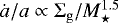 ), which roughly holds in the type I regime wherever corotation torques are weak. The outward migration regions are further shifted toward the star compared to the case of more massive disks, which impacts the resulting population of planets by a large degree since individual planets tendto pile up at the outer edge of outward migration zones, which only change on typical timescales of the disk evolution (~Myr). Furthermore, the mass at which the corotation torque saturates, which marks the upper limit of the outward migration zones, is lower for our lower-mass disks. This moves the typical mass of fast-migrating outer planets (the “horizontal branch”, Mordasini et al. 2009a) from typically ~10 M⊕ to ~3 M⊕.
For type II migration, we follow Dittkrist et al. (2014). Thus, the overall torque is proportional to ΩK ν. The alpha-viscosity  is sensitive to the temperature structure of the disk via the isothermal sound speed cs. The temperature differs for varied stellar masses due to the change of direct illumination by the star – caused by the different stellar radius and temperature – as well as due to a lower viscous dissipation rate Ėvisc. To transition from type I to type II, we use the gap opening criterion of Crida et al. (2006). Planets with masses below this critical mass are not able to carve a deep gap in the gaseous disk and are therefore moving according to type I migration. In Fig. 1, the transition can be seen at masses of 102 M⊕ to 103 M⊕ for the top panel. Moving from lower to higher planetary masses, the color code gets a visibly lighter tone corresponding to a significant migration rate drop. In the outermost disk, gas moves radially outwards which leads to an outward migration in type II (top right corner in Fig. 1) but not in type I. We observe a more pronounced transition in the bottom panel of Fig. 1, which can be explained by the much cooler disk and the different scaling of the two regimes. It thus becomes more relevant in the low-mass star disks. Furthermore, the transition location is moved to lower masses ~30 M⊕ for the bottom panel.
Overall, disk migration can take place more quickly around low-mass stars if the disk mass is the same as it is for solar-type stars. However, for typical disk masses, we expect slightly slower migration in type I and type II regimes, with outward migration occurring for smaller planets, and the relevant zones lying closer to the star.
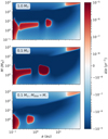 |
Fig. 1 Normalized type I and type II migration rate for three different stellar masses and disks. In the top panel, a disk with a total mass of 0.02 M⊙ around a solar mass star after an evolution of 100 kyr is displayed; the central panel shows the same disk at the same time, but the stellar mass is reduced to 0.1 M⊙ ; and the normalized migration rates for a disk with ten times less mass around a 0.1 M⊙ star can be seen in the bottom panel. Regions with most strongest colors (blue or red) are regions where migration is fastest. With scaled disk mass, the outward migration zones (red) move to lower planet masses and closer orbits. This generally causes an earlier inward migration. |
2.2 Transit radii
To better compare observed radii measured by transit surveys with radii of synthetic planets, we calculate the “transit radii” of the modeledplanets following Guillot (2010). For this purpose, we can use the internal and atmospheric structure of each planet.Simply taking the arbitrary numerical outer boundary of the structure is not appropriate. Instead, an estimate for the radius of the shadow that a planet casts when passing in front of its host star needs to be employed.
Hansen (2008) found that the optical depth along a chord is enlarged by a factor of  compared to the optical depth integrated radially outwards from a radius R. Here, γ is a factor relating the opacity in the visual to the opacity in the thermal wavelength range (Jin et al. 2014, Table 2) and H0 is the local scale height in the envelope at a given radial location.
We chose an optical depth τ = 2∕3 in our gray atmosphere as the outer Eddington boundary condition and we note that for a percent-level comparison to a particular observation, a non-gray atmosphere and the instrument specific wavelength band would have to be included. For planets without a H/He envelope, the transit radius is equal to their composition-dependent core radius calculated using a three layer model (considering iron, silicates, and whether a planet incorporates ice from outside of the iceline(s)) (Mordasini et al. 2012b).
2.3 Initial conditions and Monte Carlo variables
Owing to the statistical approach of population synthesis, we treat the initial conditions as random variables that we draw from probability distributions for each simulation. The randomized variables, called Monte Carlo variables, are the gas disk mass Mgas (sometimes expressed as initial surface density Σg at 5.2 au), the metallicity [Fe/H], the inner edge rin of the disk, a parameter scaling the strength of photo-evaporation Ṁwind, and the starting locations of the planets astart. For consistency within the paper series, we employ the values from Paper II for the case of solar-type stars and scale them with stellar mass.
Figure 2 shows for each host star mass bin, the probability distributions of the randomized variables used in this study as well as closely related, resulting quantities. While we assume that the distribution of the metallicity (Santos et al. 2003)remains the same, all other parameters scale with stellar mass. We note that M dwarfs are generally older than solar-type stars (in terms of the mean), therefore the metallicity could change with the evolution of stellar clusters. Nevertheless, we assume that this effect is small compared to other unknown scalings of the protoplanetary disks discussed below.
Apart from randomized variables, we also fix a set of parameters, which are summarized in Table 1. Importantly, we follow Paper II in setting the radius of planetesimals to 300 m and initializing the gas surface density profile as (Veras & Armitage 2004):
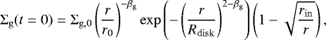 (2)
(2)
where r0 = 5.2 au is the reference distance, βg = 0.9 the power-law index (Andrews et al. 2010), Rdisk the cutoff radius for the exponential decay and rin is the inner edge of the disc.
Before discussing the individual choice of distributions for the observation-informed parameters, we note that the solar-type initial conditions of Paper II include a steeper slope for the planetesimal disk βpls than the gas disk (βpls = −1.5 instead of −0.9). This is motivated by results from planetesimal formation models (Dra̧żkowska et al. 2016; Dra̧żkowska & Alibert 2017; Schoonenberg & Ormel 2017; Lenz et al. 2019). We assume that this steepening is valid for all stellar masses and adopt a βpls = −1.5 for all simulations (except in the scenario described in Sect. 4.1.2).
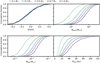 |
Fig. 2 Cumulative distributions of initial conditions and resulting quantities for different M⋆. The Monte Carlo parameters [Fe/H] and Mgas can be converted to initial solid disk masses (Msolid = 10[Fe∕H]fdg,⊙Mgas, where fdg,⊙ = 0.0149 following Lodders 2003) and disk truncation radii ( |
Model parameters.
2.3.1 Disk mass
The initial gas disk mass for solar type stars is based on the Class I disk observations Tychoniec et al. (2018) (see Paper II). Tychoniec et al. (2018) do not split their sample of Class I disks into different stellar masses, but they do mention that they observe a weak correlation with the bolometric luminosity which can be seen as a proxy for the stellar mass. However, the non-triviality of the mass-luminosity relation for very young protostars makes inferring the slope of this weak correlation a task outside the scope of this work. While sensitive to dust and not gas, the scaling of disk mass with stellar mass can be inferred from recent ALMA measurements. For more evolved disks, Pascucci et al. (2016), Barenfeld et al. (2016), as well as Ansdell et al. (2017), found a dust mass dependency on stellar mass, which is steeper than linear. These measurements cover stellar masses down to 0.1 M⊙. Therefore, they probe deep into the M dwarf class. Within the scatter of the observations, the linear slope fits well the different spectral types without any visible transition. Testi et al. (2016) and Sanchis et al. (2020) extended the observations to the brown dwarf regime and found statistically consistent results.
While Barenfeld et al. (2016) had not yet found a clear difference in slopes of the dust mass to stellar mass relation when comparing their results for Upper Sco with disk masses for the younger Lupus cluster, Ansdell et al. (2017) and Pascucci et al. (2016) reported a time dependency of the slope by enlarging the sample to more stellar clusters. These latter findings point toward a stellar mass dependent time evolution of the dust and, therefore, do not well constrain the initial dust mass. Tentatively interpolating back this steepening of the disk mass to stellar mass relation to time zero, we adopted a linear dependency of the disk mass on the stellar mass Mgas ∝ M⋆ consistent with (Andrews et al. 2013). In addition, this is in line with previous theoretical works (slopes of 0.5 to 2 in Raymond et al. 2007).
Compared to other works, these choices lead to a similar mean disk mass for the 0.1 M⊙ stars of 0.0032 M⊙ as in the “heavy disk” case of Alibert & Benz (2017). They use a stellar accretion rate informed scaling with a power of −1.2, but lower values for the solar mass stars. In Fig. 3, we compare the disk gas masses drawn for this work with those used in previous planetesimal-based population synthesis works of Ida & Lin (2005), Alibert et al. (2011), Alibert & Benz (2017), and Miguel et al. (2020). There is also a considerable agreement with the initial conditions used by Liu et al. (2020) who prescribe an accretion rate following the Orion data set by Manara et al. (2012). To get an estimate of the disk mass, they integrated the stellar accretion rate over time assuming no photoevaporation or accretion onto the planets.
As in Paper II, we then multiply the gas disk mass with spectrally measured stellar metallicities (Santos et al. 2003) to get the initial dust disk mass, which is available for the formation of planetesimals. We assume no dependency of the metallicity on the stellar mass. Additionally, an efficiency of transforming the dust to planetesimals of 100% was chosen. The planetesimal surface density is reduced at radii closer to the star if for a given element no chemical species containing it can condense out at the local disk temperature (see Thiabaud et al. 2014). This leads to sharp transitions in the surface density profile of solids, most prominently the water iceline, whose location depends on the temperature at time zero of the simulation.
2.3.2 Disk radius
Although it is challenging to measure the initial radius of the gaseous disk, trends about the disk size of – notably evolved – disks with disk mass were found by Andrews et al. (2010). The scaling relation of disk mass to disk radius follows  , which was recovered later (Andrews et al. 2018). We use this constraint to calculate the gas disk size from the randomized mass without introducing additional scatter.
For the dust disk size, a direct correlation of dust disk radii with stellar mass using ALMA data could not be found by Ansdell et al. (2018) who advocate more high-resolution CO line observations to give clearer constraints. However, it became clear thanksto the ALMA measurements that dust radii are smaller than gas radii by about a factor of 0.5 (Ansdell et al. 2018), which we adopt to truncate the planetesimal disk. The recent study of Sanchis et al. (2021) expand and confirm these results and further find no dependence of the CO to dust size ratio on the stellar mass.
With this approach, the exponential cut-off radii of gaseous disks around stars with lower stellar masses follow the relation  . The numerical values drop from a meanof 62.1 au for 1.0 M⊙ to 14.8 au for 0.1 M⊙.
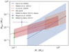 |
Fig. 3 Disk masses used in different theoretical planetary population synthesis works. Shaded regions or error bars show the 1σ scatter in the distributions. Log-uniform distributions are used to sample disk masses in all works except for Miguel et al. (2020) who draw from a linear-uniform distribution (1 × 10⁻⁴ M⊙ to 5 × 10⁻² M⊙). They are also the only work which samples over stellar masses instead of using fixed values. Liu et al. (2020) prescribe stellar accretion rates as opposed to disk masses; the data shown here corresponds to integrating from time zero to 10 Myr. The “heavy disk” case of Alibert & Benz (2017, open-circle, scatter-omitted) draws disks with twice their nominal mass. Apart from this case, we show the distributions labeled as nominal by the respective authors. The disk masses used in this work are in agreement to previous assumptions. |
2.3.3 Inner edge
The numerical inner edge rin is a free parameter of our model and a key factor in the final orbital positions of many of the innermost planets. This is especially important when comparing synthetic results to transit and radial velocity surveys which are most sensitive to the innermost region. In this section, we analyze where rin should lie as a function of stellar mass.
The physical motivation for an inner edge is a magnetospheric cavity (Bouvier et al. 2007), where ionized material of the disk is lifted by the magnetic field lines from the midplane and accreted onto the star. This typically happens at the corotation radius (e.g., Günther 2013), where the magnetic field rotates at the same speed as the gas. It is therefore reasonable to not extend the modeled disk closer to the star than its corotation radius. The order of percent sub-Keplerian speed of the gas disk is negligible for this consideration and thus we take rin at the location where the Keplerian orbital period is equal to a stellar rotation period drawn from measured distributions. We do not take into account the vaporization of silicates and ionization of the disk gas in the innermost regions of the disk.
The rotation periods of young stars can be derived from periodic variations of objects in young stellar clusters, such as the Orion Nebula Cluster (Herbst et al. 2002), NGC 6530 (Henderson & Stassun 2011), NGC 2264 (Lamm et al. 2005;Affer et al. 2013;Venuti et al. 2017), NGC 2362 (Irwin et al. 2008), and NGC 2547 (Irwin et al. 2007). Irwin et al. (2008), as well as Henderson & Stassun (2011), discuss an increasingly steep slope in the rotation period versus stellar mass diagrams with increasing age. However, for the youngest clusters (Orion and NGC 6530) no decrease of the rotation period with decreasing stellar mass was found (Henderson & Stassun 2011). Therefore, this feature can be attributed to a faster spin-up of low mass stars and is not considered an initial condition for planet formation. As initial condition, we therefore chose the same rotation periods for all stellar masses. Thus, the orbital distance of the inner edge of the disk scales at  .
.
Despite the long history of observations in the field, the exact distribution of classical T Tauri rotation periods is still subject to a lot of statistical uncertainty. Venuti et al. (2017) used data from 38 days of CoRoT observations to constrain the rotation periods in NGC 2264, which has an estimated age of ~3 Myr. As is the case with other authors (e.g. Henderson & Stassun 2011), they found that stars that still show signs of accretion (i.e., classical T Tauri stars) have slower rotation periods than diskless stars. In Fig. 4, we show the data of Venuti et al. (2017) in two mass bins for diskless and disk-bearing stars. No clear difference was found between the different masses in the case of disk-bearing stars. Therefore, we adopted a distribution of rotation periods used to constrain the inner edges following the full T Tauri sample of Venuti et al. (2017), that is, a log-normal distribution with a mean of 4.74 days and a spread σ of 0.3 dex (2.02days).
To summarize, in period space, the same distribution as of the inner disk edge is used for all stellar masses in terms of period, implying a dependency in terms of orbital distance as  . This also means that for 1 M⊙, the distribution used in Paper II is recovered.
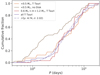 |
Fig. 4 Cumulative distribution of rotation periods of disk-bearing and diskless stars in NGC 2264 (estimated age ~3 Myr) found by Venuti et al. (2017). An error function corresponding to the normal distribution with the indicated mean and standard deviation was fitted to the logarithm of the rotation periods of all T Tauri stars (dash-dotted line). This distribution defines the corotation radius, which we set as the inner disk edge. |
2.3.4 Initial embryos
The initial seeds of planetary growth, called embryos, are placed randomly into the protoplanetary disk at t = 0 starting from the inner edge of the disk, rin, out to an upper limit. In Paper II, the upper limit is chosen to be 40 au, which we adopt for the solar-mass populations. This outer edge is then multiplied with  . Therefore, it is kept at fixed orbital period. Many timescales relevant to planet formation, such as the growth timescale of the core by planetesimals, scale with the orbital period. This motivates the move to keep it the same for better comparability amongst the populations.
Based on simulations of runaway planetesimal accretion and beginning of oligarchic growth (Kokubo & Ida 1998; Chambers 2006), the locations of the initial embryos are drawn from a log-uniform distribution between these two boundaries. If a planet would be placed within 10 Hill radii of an already placed embryo, a new location is drawn.
We chose to place 50 embryos into each protoplanetary disk at time zero of our simulations. This is a compromise because placing more embryos leads to longer simulation times. The influence of the number of initial embryos is studied in detail in Paper II. For the simulations shown in Sect. 4.1.2, we do single-embryo calculations.
As in Paper II, the initial mass of the embryo is set to be 10−2 M⊕. This mass is not scaled with the stellar mass, which is a choice that changes the initial mutual Hill spacing with varying stellar mass and thus the gravitational interactions between the embryos (see the discussion in Sect. 4.4).
2.4 Disk observables
2.4.1 Disk lifetime
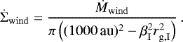
Although the disk lifetime is not a direct Monte Carlo variable, it depends strongly on the photo-evaporation variable Ṁwind. We follow Matsuyama et al. (2003) and remove mass with an equal rate per area due to FUV radiation from different stars (external) as:
 (3)
(3)
This is applied outside of a modified gravitational radius 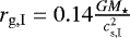 (see Alexander et al. 2014, for a discussion of the prefactor), where cs,I is the sound speed of dissociated hydrogen at a temperature of 1 × 10³ K. The amountof external photo-evaporation would depend on the proximity to more massive stars. Here, we consider this as a free parameter (see e.g., Haworth et al. 2018, for a more modern approach to constrain it).
We choose Ṁwind such that the distribution of the lifetimes of the synthetic disks is in agreement with observations, as can be seen in Fig. 5. For that, we keep the unknown viscous α parameter at α = 2 × 10⁻³ for all stellar masses. By construction, the lifetimes of the different stellar mass bins are similar. Disk lifetimes obtained from observed fractions of disk-bearing stars in young stellar clusters (Strom et al. 1989; Haisch et al. 2001; Mamajek et al. 2009; Fedele et al. 2010; Ribas et al. 2014; Richert et al. 2018) are sensitive to the pre-main-sequence evolution model of the stars used to determine the cluster age (Richert et al. 2018). Therefore, a larger uncertainty than the empirical scatter results.
In Fig. 5, we show the results of Richert et al. (2018), who used three different pre-main-sequence evolution models to get typical disk lifetimes varying by more than a factor of two. For comparison of the modeled disk lifetimes to measurements, it is necessary to estimate the time during which a simulated disk would be detected by typical survey used to get the observational data. We follow Kimura et al. (2016) to consider a disk as dispersed at the moment the disk becomes transparent (optical depth smaller than unity, τ = κΣg∕2 < 1, where κ is the Bell & Lin 1994 opacity) everywhere in the region where Tmid > 300 K. This is a broad estimate for near-infrared observations, which are the basis of disk lifetimes studies. For low-mass stars, this observable disk lifetime substantially differs from the different criterion used in Paper I and Paper II, where the disk is considered to be dispersed at the moment the total mass Mgas < 1 × 10⁻⁶M⊙ or when the surface density is Σg < 1 × 10⁻³g cm−2 everywhere in the disk.
Given the large uncertainty in the age determination of the clusters, our modeled disks reproduce the observations to a satisfying degree. However, there is a lack of short-lived disks for some clusters. Nevertheless, the scatter is very large at early times, indicating that the environments where the stars are born play a large role and should be investigated in the future.
Regarding the dependency with stellar mass, Richert et al. (2018) do not find a significant difference when going from solar mass stars to lower stellar masses. Therefore, we assume that the lifetime of disks does not depend strongly on the stellar mass. We point out that there is a clear dependency of the lifetime of a disk on stellar mass when looking at M⋆ > M⊙ (Haisch et al. 2001; Ribas et al. 2015), but we are not aware of any reason to extrapolate this dependency to lower stellar masses given the lack of observational evidence.
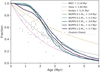 |
Fig. 5 Fraction of disk-bearing stars as a function of time. Both observational data assembled by Richert et al. (2018), as well as the synthetic lifetimes for different stellar masses, are shown. The age determination of clusters is sensitive to the employed pre-main-sequence model. The observational data and an exponential fit to it is shown using the age scale from Siess et al. (2000) as well as fits to the same cluster data but using the dating of Feiden (2016) and the MIST collaboration (Choi et al. 2016). |
2.4.2 Stellar accretion rates
Similarly to the observed lifetimes, stellar accretion rates have to be matched by the simulated disks (Manara et al. 2019). The process driving accretion rates in the simulations is the viscous evolution. Numerically, we take the disk gas mass that flows into the innermost numerical cell as gas accretion onto the star Ṁacc. In general, thisflux is not radially constant in the disk due to it not being in equilibrium at all times (Eq. (25) in Mordasini et al. 2012b).
In Fig. 6, we show the resulting Ṁacc of our synthetic populations for the various stellar masses at two different times. This can be compared to the Lupus data obtained by Alcalá et al. (2017). For planet formation, the most important stages are early in the disk evolution when most of the mass is still present. Therefore, a comparison to clusters older than Lupus (1–3 Myr) would not be as relevant.
We find mass accretion rates on the same orders of magnitude as were observed in Lupus. The intrinsic scatter of the synthetic populations is lower than in the observed sample. This is a known discrepancy between simple models using a single viscous α value (2 × 10⁻³ in our case) and observations (see for example Rafikov 2017 or Manara et al. 2020 and references therein). Furthermore, the evolution with time seems to be rather rapid compared to observations, given that at 3 Myr, a lot of the more massive stars have already accreted most of the disk mass. We note that we consider here our numerical simulation time: realistic cluster ages would include the early star formation stages, which can lead to a shift of a few 100 kyr. The scaling of Ṁacc with stellar mass in the synthetic work is more shallow than the fitted observational data. An in-depth comparison of disk properties to disks resulting from population synthesis work that extends the approach of Manara et al. (2019) will be addressed in a future paper.
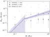 |
Fig. 6 Stellar accretion rates of observations and synthetic disk populations as a function of stellar mass. For the synthetic data points at two different times (colored crosses and large dots), the mean of the distribution is plotted and the standard deviation is indicated with error bars. The observational data (small points and triangles for upper limts) and the broken power-law fit with its estimated errors is taken from Alcalá et al. (2017) for the Lupus cluster (estimated age of 1–3 Myr). The break for this particular fit was chosen to lie at 0.2 M⊙ (motivated by Vorobyov & Basu 2009). |
3 Results
We now turn our attention from disk initial conditions and parameters for the given stellar masses to the resulting synthetic planetary population. To help identify the different simulations, we list in Table 2 the identifiers and stellar masses of the different simulations discussed here. We present our results as a function of the stellar mass focusing on the type of planets that form (Sect. 3.2), the mass – semi-major axis plane (Sect. 3.1), planetary mass functions (Sect. 3.3), and planet radii and compositions (Sect. 3.4).
Overview of the simulation names, stellar masses and effective temperatures, number of initial embryos Nemb,ini, and number of simulation runs for all simulations discussed in this work.
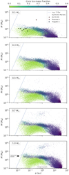 |
Fig. 7 Synthetic populations of planets as a function of a and M with summed-up mass fraction of all ice species in the planetary core in color. Their NGPPS identifiers are NGM10, NGM14, NGM11, NGM12, and NG75. Some observed planets around very low-mass stars are shown (Anglada-Escudé et al. 2016; Morales et al. 2019; Agol et al. 2021). Planet masses increase with host star mass, but no giant planets occur for M⋆ < 0.5 M⊙. The radial position where the tidal orbital decay timescale reaches 5 Gyr is indicated. |
3.1 Mass-distance diagrams
The mass-and-semi-major axis diagrams of the populations are shown in Fig. 7. Each system starts with 50 embryos of 0.01 M⊕ which collide over time, thus the number of points in each of the plots is on the order of 20 000. The composition measured by the volatile- or ice-mass fraction in the solid core of the planets is color-coded.
General trends for all stellar masses are as follows. First, the ice-rich planets at large semi-major axes. This population is dominated by low-mass planets and the high ice content is an imprint of the lower local temperatures. Second, the effect of migration visibly brings ice-rich planets at Earth to super-Earth masses closer to the stars. Lastly, we identify a distinct population of giant planets that is separated by a runaway gas accretion desert (Ida & Lin 2004a) from the solid-dominated population.
Although these features can be seen for all the different stellar masses, there are clear differences between the populations, which show the influence of the reduced stellar and disk mass. A first feature is that the “horizontal branch” (Mordasini et al. 2009a), a population of icy super-Earths that migrated toward the star in the type I regime, is located at different planetary masses. In Fig. 7, it can be identified by the blue colored points at small semi-major axes and is marked in the bottom panel. The origin of the difference between the stellar masses can be explained as follows: Given a lower disk mass, the corotation torque saturates and planets start migrating at lower planetary masses (see Sect. 2.1). Thus, the population of close-in, ice-rich planets extends to lower masses for the lower stellar mass populations (down to ~1 M⊕ for the 0.1 M⊙ population NGM10 instead of down to only ~3 M⊕ for the solarmass case, NG75). However, the scatter is quite large and to assess this in a more quantitative way, a larger set of statistics would be needed, especially for the low stellar mass case, where few ice-rich planets migrated to the inner parts of the disk.
A second distinct trend with the stellar mass is a reduction of the number of giant planets with decreasing stellar mass (Laughlin et al. 2004, see also Sect. 3.2.1 for a quantitative discussion). Interestingly, the semi-major axis distribution of the giants differs quite a bit when comparing the 0.7 M⊙ (NGM12) case with the 1.0 M⊙ (NG75) case. Giant planets are more frequently scattered for the more massive case, since there is more often a second or third giant planet forming, which then leads to more frequent interactions. Therefore, the distribution of giants in NGM12 is more localized at around 1 au compared to the solar-mass case. In the lowest stellar-mass population, not a single giant planet was able to form.
Another quite weakly accentuated feature due to little statistics is an under-density due to tidal migration at very close orbits of a few 10−2 au, where tides push some planets into the star and leave a void of massive, close-in planets. This can be seen as a fuzzy diagonal cut-off in the mass-and- semi-major axis diagram, which increases to higher planetary masses with increasing semi-major axis (Schlaufman et al. 2010; Benítez-Llambay et al. 2011).
Additionally, all populations show a similar “triangle of growth” at very low planetary masses indicated in the bottom panel of Fig. 7. This absence of planets means that there is a region where embryos grow for all sampled disk conditions. The region spans from 0.1 to 10 au, which are the regions most favorable for planetesimal accretion where growth timescales are short and feeding zones large enough for planetary growth to occur.
Overall, we recover with the use of the mass-distance diagrams, the expected trends of fewer giant planets with decreasing stellar mass and the imprint of stellar mass dependent migration. The observed masses of the TRAPPIST-1 system (Gillon et al. 2017) as well as Proxima b (Anglada-Escudé et al. 2016) are reproduced. However, this is not the case for the recently discovered giant planet orbiting the late (M5.5) M dwarf GJ 3512 (Morales et al. 2019). This warrants further discussion in Sect. 4.1.2. After this qualitative first look at the results, we present a quantitative analysis of planetary types and masses in the following sections.
3.2 Types of planets
As a second step to explore the synthetic populations of planets around different host star masses, we categorize the planets into the following groups:
-
Planets with masses larger than Earth (M > 1 M⊕)
-
Earth-like planets defined as planets with masses ranging from 0.5 M⊕ to 2 M⊕
-
Super Earths (2 M⊕ to 10 M⊕)
-
Neptunian planets (10 M⊕ to 30 M⊕)
-
Sub-Giants (30 M⊕ to 100 M⊕)
-
Giant planets (masses larger than 100 M⊕).
Additionally, we add a category of temperate, Earth-mass planets that are introduced and discussed in Sect. 3.2.4.
Compared to the analysis performed in Paper II, the categories are identical with the exception of including the few brown dwarf mass planets as giant planets and choosing a different temperate zone. The distinction of giants and core-accretion brown dwarfs is not relevant for the purpose of this paper and the second change is introduced because accounting consistently for the scaling of the temperate zone with stellar mass requires the use of a more complex model.
For the following analysis, we use the term fraction of systems, fs, as defined by the ratio of systems containing one or more planets of a given planetary type divided by the total number of simulated systems Nsys,tot. The occurrence rate pocc of a planetary type is the number of formed planets of this kind in any simulated system divided by Nsys,tot. The ratio pocc∕fs results in the mean multiplicity, that is, the mean number of this type of planet per system. The resulting fs for the different planetary types are shown in Table 3 and their mean multiplicity is shown in Table 4. Additionally, a visual representation of the same data also including pocc is shown in Fig. 8. To get an idea of the dynamics, the eccentricities of the different types can be found in Table 5 and the host star metallicity [Fe/H] in Table 6 and in the bottom right panel of Fig. 8. The metallicity is calculated based on the drawn dust to gas ratio fdg (see Sect. 2.3.1) which thentranslates to ![Mathematical equation: $[\mathrm{Fe}/\mathrm{H}] = \log_{10} \left(f_{\textrm{dg}} / f_{\textrm{dg},\odot} \right)$](/articles/aa/full_html/2021/12/aa40390-21/aa40390-21-eq18.png) , where fdg,⊙ = 0.0149 (Lodders 2003).
, where fdg,⊙ = 0.0149 (Lodders 2003).
Fraction of systems with specific planetary types for the different stellar mass populations with initially 50 lunar-mass embryos.
Multiplicity of specific planetary types for all populations.
Mean eccentricities of different planetary types for all populations.
3.2.1 Giant planets
As can be seen in Table 3 and Fig. 8, the giant planet occurrence drops with increasing stellar mass in our simulations. No planets with masses above 100 M⊕ form around stars with masses below 0.5 M⊙. At this transition stellar mass, the synthetic population with nominal parameters contains only 21 giant planets in 16 systems.
At 1 M⊙, 17% of the stars have one or more giant planets (see also Paper II). This is in agreement with observational estimates (14% were found by Mayor et al. 2011). This planet type shows a clear preference for high stellar metallicities, with a mean of about 0.15 for all stellar masses where giants can form. We can thus recover the well-known observational result (e.g. Santos et al. 2003). Additionally, giant planets are characterized by rather significant eccentricities (~0.15) compared to lower-mass planets, and a rather low multiplicity (~1.4), again compared to super-Earth and Earth-like planets.
In Sect. 4.1, we discuss the trends with respect to previous literature. Furthermore, in light of recent discoveries of massive planets around low-mass stars, we explore possible ways to increase the giant planet occurrence rate.
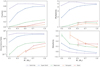 |
Fig. 8 Fraction of systems, multiplicity, and occurrence rate for five planet-mass categories as a function of the stellar mass. The standard error of the mean is indicated. Where necessary, the markers are slightly shifted in x-direction to better distinguish them. |
Mean metallicity [Fe/H] of stars hosting specific categories of planets.
3.2.2 Neptunian planets and sub-giants
The frequency of simulated Neptunian planets and Sub-giants declines with decreasing stellar mass. The slope is steeper for smaller masses where these kind of planets become very rare. In strong contrast to the Earth-like and super Earth planets, Neptunian planets and sub-giants are both most commonly the only ones of their kind in a system and their orbits are more eccentric than those of other types, which holds for all stellar mass bins.
The orbits of sub-giants are more eccentric than those of Neptunian planets. This does not seem to be the case for the lowest stellar mass where sub-giants emerge. However, more statistics would be required to make a strong point because only ~5 simulations exist where sub-giants formed around 0.3 M⊙ stars. For stellar masses larger than 0.3 M⊙, sub-giants are present in 5–10% of the systems.
For both sub-giants and Neptunian planets, the mean metallicity of their host stars decreases with increasing stellar mass.
3.2.3 Earths and super-Earths
We find that in our synthetic populations, Earth-like planets are most common around stars with a mass ranging from 0.3 M⊙ to 0.7 M⊙ and – conversely to the initial solid mass trend – become less frequent around stars with masses above 0.7 M⊙. In contrast, the frequency-peak for Super Earths lies at the highest stellar mass bin (1.0 M⊙). However, the frequencies of super-Earths are very similar for the two highest stellar mass bins, pointing to a flattening of the curve, much like in the Earth-like planet case.
Similarly, the multiplicity keeps increasing for super-Earths but peaks for Earth-like planets. The highest multiplicities of Earth-like planets are present for 0.3 M⊙–0.5 M⊙, which is lower compared to the stellar mass where this planet type is most common.
The culprits associated with the decreasing trend are the giant planets ofsuch systems. As discussed in Schlecker et al. (2021), the presence of giant planets often leads to dynamical instabilities that end up removing smaller planets from the system. This is reflected in the combined occurrence rates of Earths and super-Earths: for stars with M⋆ > 0.5 M⊙, they range from 7.9 to 9.1 in systems without giant planets but are lowered to 2.4 to 2.7 if a giant planet is present.
Most of the Earth-like planets and super-Earths are on relatively circular orbits. However, the eccentricity scatter is of the same magnitude as the mean. A trend toward lower eccentricities for higher stellar masses can be seen.
In terms of host star metallicities, high metallicity is required to form Earth-like planets or super-Earths around the very-low-mass stars, whereas for stellar masses larger than 0.5 M⊙, the mean metallicity of Earth-like planet and super-Earth hosts is close to the mean of the whole population. This outcome indicates that growth to these masses is not limited by the available amount of solids at the higher stellar masses. For all the terrestrial planets, the mean metallicity decreases monotonically over the stellar mass range. This decrease can be attributed to either or both of: (a) disks containing enough solid mass to form the planetary types at lower metallicities; or (b) the destruction by scattering or ejection of planets due to the presence of more massive planets around high-metallicity stars. Given the absence of giant planets around low-mass stars, the former is sure to be the driver for the metallicity dependency there. On the other hand, the presence of giants plays an important role in disks where they can form (M⋆ ≥ 0.5 M⊙).
3.2.4 Earth-mass planets in the temperate zone
There is a wealth of processes that have to be assessed in order to constrain the habitability of planets around low-mass stars (Kaltenegger 2017). In particular, the activity levels of M dwarfs are elevated, which might inhibit the emergence of life (see the review of Shields et al. 2016). Nevertheless, constraints on the frequency of planets on which life similar to Earth has a chance to emerge is of interest. We can assess whether liquid water may exist on the surface of the synthetic planets using either mass or radius limits and select orbital separations according to the maximum and runaway greenhouse limits by Kopparapu et al. (2014). For simplicity, the reported dependence of the zone on the planetary mass is not taken into account. Instead, the limits used are those calculated for masses of 1 M⊕. We note that the parameters in Kopparapu et al. (2014) differ on a ~5% level compared to the parameters in Kopparapu et al. (2013b,a). Furthermore, the authors suggest avoiding the use of the moist greenhouse limit presented in Kopparapu et al. (2013b) due to large differences to other works. For this reason, we chose the runaway greenhouse limit as the inner boundary.
The temperate zone defined in this way moves with time based on the luminosity and the radius evolution of the star, for which we use the evolutionary tracks of Baraffe et al. (2015). In this module of the code, we use identical luminosities and radii for each stellar mass at all times. The resulting temperate zone limits after 5 Gyr of evolution are:
-
0.03–0.06 au for 0.1 M⊙
-
0.11–0.21 au for 0.3 M⊙
-
0.20–0.38 au for 0.5 M⊙
-
0.39–0.72 au for 0.7 M⊙
-
0.96–1.70 au for 1.0 M⊙.
Thus, the temperate zone moves with increasing stellar mass from orbital periods on the order of days for 0.1 M⊙ stars to orbital periods on the order of years for Solar-type stars. In our simulations, this implies that the zone is displaced from close to the former inner edge of the disk to the proximity of the former disk snowline.
An interesting pattern can be seen for the fraction of systems with Earth-sized planets in the temperate zone (see Fig. 9): The stellar mass with the highest fraction of systems with temperate, low-mass (potentially habitable) planets is 0.5 M⊙ when using the nominal mass cuts. This peak can be partially attributed to the general trend of higher occurrence of Earth-like planets around these stars (Sect. 3.2.3) as well as to the shift of the temperate zone toward less massive hosts.
However, the multiplicity keeps increasing with stellar mass (Table 4). This can be expected as the width of the temperate zone increases monotonically from 25 to 44 Hill radii (Eq. (4)) of Earth-mass planets from 0.1 M⊙ to 1.0 M⊙. Therefore, there is more dynamical space available to accommodate objects. Despite that, the occurrence rate retains a peak at 0.5 M⊙; although, the data is consistent with a constant occurrence for M⋆ > 0.5 M⊙ within confidence intervals.
In addition to the data based on cuts in planetary mass, Fig. 9 also employs cuts based on the planetary radii used in the works of Dressing & Charbonneau (2015) and Bryson et al. (2021). The difference in the occurrence rates for the varied ranges in radii and masses can be explained by the fact that in the simulations around solar mass stars, many planets in the temperate zone contain ices or are enveloped in gas. Therefore, their radius is increased and they no longer fall in the radius selection despite having a mass below 5 M⊕. The number of hydrogen-bearing planets is much lower for lower stellar masses due to lower mean masses and the proximity to the star. This shifts the most common temperate planet host to lower stellar masses (0.3 M⊙).
Due to the dynamically distinct locations of the temperate zone, we do not expect the respective planets’ eccentricity to be similar. Indeed, a trend toward lower eccentricities with increasing stellar mass is recovered (see Table 5). In terms of mean host-star metallicity (bottom panel of Fig. 9), a similar picture as for the Earth-like planets emerges with increased mean metallicities for low-mass stars and reduced metallicities for solar-type stars. This has strong implications for planetary searches aimed at maximizing the yield of potentially habitable planets.
Here, we put these results into context with existing observational constraints. For Earth-like planets with radii ranging from 1 R⊕ to 1.5 R⊕, which corresponds to the blue line in Fig. 9, Dressing & Charbonneau (2015) derive an occurrence rate of  around cool stars (Teff < 4000 K). For their larger, super-Earth size bin ranging from 1.5 R⊕ to 2 R⊕ (green line in Fig. 9), they report
  . Our synthetic occurrence rates with 0.24 and 0.09 for Earth-analogues and super-Earths respectively around 0.3 M⊙ and 0.25 and 0.09 for 0.5 M⊙ lie within error bars. This very precise match is quite contrasting to the overestimation of general occurrence rates reported by Mulders et al. (2019).
Recently, Bryson et al. (2021) find consistently increasing habitable zone occurrence rates with stellar effective temperature in the range of 3900–6300 K. The size limits they chose correspond to the orange line in Fig. 9 (0.5 R⊕–1.5 R⊕). Although the uncertainties derived by Bryson et al. (2021) are quite large, an increasing trend of temperate planet occurrence with stellar effective temperature is apparent. The authors note, however, that it is weaker than expected from pure geometrical enlargement of the habitable zone with stellar temperature. Furthermore, they chose the optimistic habitable zone limits (Kopparapu et al. 2014) to discuss the stellar temperature dependency, which increases this enlargement of the habitable zone with stellar mass. In contrast to their findings, in our simulations, there is an opposite clear decreasing trend of occurrence rates with stellar mass in the range considered by Bryson et al. (2021). This trend is dominated by the population of small planets ranging from 0.5 R⊕ to 1.0 R⊕. The skewness of the distribution of planetary radii especially around lower-mass stars makes the comparison to observations that favor the detection of larger planets statistically more challenging. Altogether, if future studies confirm the increasing occurrence trend of temperate planets with stellar mass, the existence of such a numerous sub-population of smaller planets needs to be reevaluated.
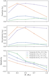 |
Fig. 9 Fraction (upper), occurrence rate (middle), and mean host-star metallicity of synthetic planets with masses or radii similar to Earth in the temperate zone (Kopparapu et al. 2014). The error-bars depict the standard error of the mean. The cuts based on radii are the same as in Dressing & Charbonneau (2015) and Bryson et al. (2021). The resulting f⊕ and η⊕ sensitively depend on this choice. |
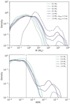 |
Fig. 10 Kernel-density estimates of the close-in (P < 300 d) planetary mass distribution (top) and the planetary to stellar mass ratio (bottom) for populations of planets around different stellar masses. The bandwidth of the Gaussian kernel was chosen following the Normal reference rule (Scott 1992). Top panel: the population around solar-type stars is shown three times: once in full, once only including planets that started within (i.e., a(t = 0) < 2 au), respectively, outside 2 au. In the bottom panel, the break in the distribution at qbr = 2.8 × 10⁻⁵ that was found by Pascucci et al. (2018) is depicted as a gray, vertical line. |
3.3 Planetary mass distribution
Because some regions at lower planetary masses in Fig. 7 are saturated with points, we derive kernel-density estimates of the probability distribution of the synthetic planets’ masses for better visibility and comparability. The resulting distribution of planetary masses and planet to star mass ratios for different stellar masses are shown in Fig. 10. For better comparability with results from the Kepler mission, we only include planets with periods P < 300 d.
Starting at low planetary masses, the density estimates increase up to a plateau spanning from 0.1 M⊕ to 10 M⊕. The plateau-like shape originates from two more narrow distributions of planets originating from further out and those growing at small orbital distances. This is revealed by splitting the population for 1.0 M⊙ at initial locations of 2 au. For lower stellar masses, the same pattern can be found, but the relative contributions of the two subsets varies.
Moving on to larger masses, there is a gap in the distribution at 100 M⊕ before giant planets become more frequent at larger masses. The exact shapes of the distributions of giant planets are influenced by low-number statistics and should not be interpreted quantitatively. Qualitatively, most giants originated from outside 2 au and we find thatthe number of giant planets increases with stellar mass.
Similar patterns can be seen in the planet to star mass ratio q distribution. It becomes clear that the distributions are not exactly overlapping. Instead, the population of small mass planets is shifted to slightly larger q around lower-mass stars. Such a trend is not in agreement with the studies of Wu (2019) and Pascucci et al. (2018), who found no dependency on the stellar mass in the Kepler database We investigate in greater detail the origins of the mass distribution in Sect. 4.2 and make a comparison with the observations in Sect. 4.3.
3.4 Planetary composition and radius
Even though the mass of a planet is the more fundamental parameter in terms of formation, transit measurements are sensitive to the radius of the planets. Therefore, we use the structure of the modeled planetary hydrogen-helium envelopes to calculate planetary transit radii following the prescription outlined in Sect. 2.2.
Figure 11 shows the masses and derived transit radii of the synthetic planets with P < 300 d for the populations NGM10, NGM14, and NGM11 with respective stellar masses of 0.1 M⊙, 0.3 M⊙, and 0.5 M⊙. The red markers show the observational data from the NASA Exoplanet Archive, where only planets with relative errors in radius, mass and stellar mass lower than 50% are included. For stellar masses below 0.2 M⊙, shown in the top panel, the planets that are shown are GJ 1132 b (Bonfils et al. 2018), GJ 1214 b (Harpsøe et al. 2013), and LHS 1140 b and c (Ment et al. 2019). Outside the shown parameter space, the object 2MASS J02192210-3925225 b found by direct imaging close to the brown dwarf limit (Artigau et al. 2015) is listed in the archive. Objects like this, with large planet-to-star mass ratios, probably formed in a process more similar to binary formation than planet formation (as in Bate 2012). Additionally, the TRAPPIST-1 system is included with masses based on Agol et al. (2021) and with the color-coded ice mass fraction derived assuming an iron core mass fraction of 32.5%.
For the 0.3 M⊙ case, we selected observed planets around stars ranging from 0.2 M⊙ to 0.4 M⊙. The two datapoints with remarkably small errors at dynamically estimated masses of 5.77 ± 0.18M⊕ and 7.50 ± 0.23M⊕ are the two planets orbiting K2-146 (Hamann et al. 2019). Given incident fluxes above 10 S⊕, their precisealignment with the ice-rich, envelope-free, synthetic planets might be a coincidence.
Concerning the synthetic data, the two straight lines at the low-mass end in Fig. 11 correspond to the compositions of pure rocky or ice-rock mixture with ~50% ice, which isthe typical ice fraction of planetesimals outside the water iceline (Thiabaud et al. 2014; Marboeuf et al. 2014). Only a small sub-population has ice fractions in between the two limiting cases. This group of planets accreted a significant amount of mass originating from outside and inside the water iceline. We see, however, that there are more of these planets for the low-stellar-mass cases due to fast type I migration at lower planetary masses. Migration of icy, far-out planets naturally leads to mixed compositions if the embryos reach the inner regions of the disk. For more massive stars, most planets only migrate at ~10 M⊕, where they can already accrete a light envelope, which leads to a significant increase in radius. For lower-mass disks, migration starts at lower planetary masses, where no significant envelope can be kept (see Sect. 2.1). Thus the 0.1 M⊙ population NGM10 includes more intermediate-composition planets without hydrogen-helium envelopes.
Overall, the resulting planets follow roughly speaking the observational data – where available – in terms of their mass-radius distribution.An exception are the outliers 2MASS J02192210-3925225 b (Artigau et al. 2015) and – although of unknown radius – also GJ 3512 b (Morales et al. 2019). Furthermore, the population of ice- and hydrogen-rich planets is not observed (see also the discussion in the next section). In the future, objects discovered by TESS and characterized using follow-up programs will populate the mass-radius diagram for low-mass stars and will help to better validate the internal structure and envelope models.
In general, the statistical distribution of planetary radii in Fig. 12 shows features that are very similar to the features seen in mass-space distribution (Sect. 3.3). The main difference is that the planets do not span over many orders of magnitude in radii due to the degeneracy in the radii of giant planets (maximum at R ~ 13 R⊕) and the dependency of radii on masses (~M1∕3).
The synthetic radius distribution in Fig. 12 shows hints of two radius valleys for the higher stellar masses (0.5 M⊙–1.0 M⊙). In contrast, only a single valley is found in the observed population of planets (Fulton & Petigura 2018). A single valley was also predicted by photo-evaporation (Owen & Wu 2013; Lopez & Fortney 2013; Jin et al. 2014). Alternative explanations are core-driven mass loss (Ginzburg et al. 2016), impacts (Wyatt et al. 2020) or the formation itself (Venturini et al. 2020).
It is striking that the two synthetic valleys in our simulations are located to either side of 2 R⊕, where the observed gap is found. This is related to the presence of several synthetic, ice-rich planets close to the inner edge of the disk. As shown by Jin & Mordasini (2018), hydrogen-free, icy cores populate the radius distribution at exactly the location where the observed radius valley is located. However, the radii would change if a vapor phase in hot, water-rich atmospheres was included (Turbet et al. 2020, see also Venturini et al. 2020 for a work including this effect). Furthermore, too efficient envelope stripping for colliding embryos could re-populate the gaps. We will address this in more detail in a future work.
The observed gap shows an interesting stellar mass dependency (Fulton & Petigura 2018; Wu 2019). Due to the general mismatch, we cannot directly compare it to our simulations. Additionally, the sizes of the super-Earths (i.e., the planets below the radius gap) and the sub-Neptunes (i.e., above the gap) were individually analyzed in Fulton & Petigura (2018) and both show a trend of increasing mean size with increasing stellar mass. We note that their sample extends to only 0.8 M⊙ and not to M dwarfs. This is in agreement with our synthetic data, where there is a clear trend toward larger mean size for the sub-Neptunes around more massive stars.
An interesting feature at lower radii is that the planet occurrence rate pocc of planets at a specific radius is higher for lower-mass stars. Mulders et al. (2015) show the same trend for the observed Kepler sample. However, they find higher occurrence rates by factor of 3.5, whereas we only find differences on the 10% level, with the trend stopping at 0.5 M⊙.
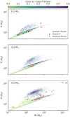 |
Fig. 11 Populations of synthetic planets as a function of planet mass and transit radius. Only planets with orbital periods P < 300 d are included. The core ice mass fraction is shown in color and observational data from the NASA Exoplanet Archive (accessed 8.3.2021) is over-plotted in red for comparison. |
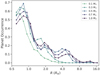 |
Fig. 12 Occurrence rates (pocc = Nplanets∕Nsystems) of synthetic planets on orbits with periods P < 100 days as a function of their transit radii. The data is binned and bin centers are connected and marked with squares for better visibility. |
4 Discussion
4.1 Giant planet occurrence for different stellar masses
The best constrained occurrence rates for planets with known masses exist for giant planets, which are most readily detectable. In general, the frequency of giant planets increases with stellar mass (Endl et al. 2006; Butler et al. 2006; Johnson et al. 2007, 2010; Gaidos et al. 2013; Montet et al. 2014) up to an inversion at high stellar masses (~2 M⊙, Reffert et al. 2015).
4.1.1 Solid mass limited growth
At least for stellar masses below this inversion, the increasing trend is well explained by works on giant planet formation based on the core accretion paradigm. Adams et al. (2004) report fast external evaporation of disks around M dwarfs, effectively reducing the available gas to form giant planets. Even without this effect, Laughlin et al. (2004) found much slower growth timescales at a fixed semi-major axis around a 0.4 M⊙ star, mainly due to the reduced solid surface density and the longer orbital timescale, which is also one of the conclusions of the population synthesis work by Ida & Lin (2005) and Alibert et al. (2011). The latter study stresses the importance of the disk mass on the resulting population of planets. As in this study, these works nominally assumed more massive protoplanetary disks around more massive stars motivated by measured stellar accretion rates. In general, we recover the same trends of low giant planet frequencies around low-mass stars (see Fig. 8). The reasons for this are attributed to the growth being limited by fast type I migration and long solid accretion timescales.
In a quantitative scope, Alibert et al. (2011) were able to approximate the synthetic giant planets resulting from their single-embryo populations around different stellar masses by scaling the distribution resulting from the 1 M⊙ case. They found planetary masses  with γ = 0.9 in their nominal case (disk mass
  ). The same cannot be recovered in our simulations, where the giant planet distribution seems to peak at the same planetary mass for all stellar masses. The overall frequency of giants is reduced but not their mean mass. However, we stress that our data set is much more sparse since only 1000 stars (each starting with 50 embryos) and about 100 resulting giant planets were simulated compared to the 30000 stars each with a single embryo in Alibert et al. (2011). Therefore, it is possible that some trends are hidden in statistical noise. If there is indeed no dependency of the mean giant planet mass on the stellar mass, N-body effects – such as the ejection of planets – might have played an important role in influencing the mass function in the newer simulations. A dedicated future paper in this series will focus on this point.
The trend toward fewer giant planets with decreasing stellar mass is also found in the study using pebble accretion instead of planetesimals by Liu et al. (2019). Although the growth in that case is no longer limited by the accretion timescale, which is shorter in the pebble accretion scenario, the pebble isolation mass decreases with stellar mass. Therefore, planets do not grow above ~5 M⊕ around starswith masses <0.3 M⊙. At such low planetary masses, gas accretion is still inefficient. This transition stellar mass is similar to our value of 0.5 M⊙ considering that only few ~100 M⊕ objects formed at this mass in the simulations from Liu et al. (2019).
Overall, we highlight the fact that despite the range of different models and assumptions about the initial conditions, a number of works recovered the trend of a decreasing number of giant planets for decreasing stellar masses: an insufficiently small solid mass reservoir leads to starved growth which, in turn, inhibits subsequent gas accretion. This indicates that this is a very robust prediction of the core accretion scenario of planet formation.
4.1.2 Massive planets around low-mass stars
Even though giant planet occurrence rates do increase with stellar mass, quite a number of systems with giant planets in orbit around M dwarfs of 0.3 M⊙–0.4 M⊙ exist. The first M dwarf known to host planets is GJ 876 (Marcy et al. 1998, 2001; Delfosse et al. 1998; Rivera et al. 2005, 2010; Millholland et al. 2018), where now four companions have been confirmed. Two of them are giant planets (with masses of 1.95 MJup and 0.6 MJup), orbiting a 0.37 M⊙ star (von Braun et al. 2013). Other examples are GJ 849 (0.65 M⊙ Stassun et al. 2016) with two giants (Butler et al. 2006) of masses 0.77 MJup and 0.9 MJup (Montet et al. 2014); GJ 179 a 0.36 M⊙ star hosting a giant planet with a mass of 0.8 MJup (Howard et al. 2010); and GJ 317 (0.42 M⊙ Anglada-Escudé et al. 2012) hosting a potentially up to 2.5 MJup massive planet and a second giant with Msini = 1.6 MJup (Johnson et al. 2007; Anglada-Escudé et al. 2012).
Below stellar masses of 0.3 M⊙, no stars hosting giants were found1 until the recent discovery of GJ 3512b, a planet with a minimum mass of 0.463 MJup around a 0.123 M⊙ star (Morales et al. 2019), which poses the biggest challenge to all current planet formation scenarios. Additionally, it is quite likely that a Saturnian mass companion leads to an inner cavity in the transition disk CIDA 1 (Pinilla et al. 2018).
In our nominal populations presented in Sects. 3.1 and 3.2, we do not find giant planets around stars with masses below 0.5 M⊙. As a consequence, in order to form a planet like GJ 3512b, either the physical parameters are to be revised in our models or different physical processes are at work, such as a different formation channel (gravitational instability). Therefore, we explore variations of parameters in the Bern Model to increase the efficiency of core-accretion planet formation around low-mass stars. To this end, we chose a stellar mass of 0.1 M⊙ to model conditions similar to GJ 3512b (M⋆ = 0.123 ± 0.009 M⊙).
One trivial pathway to form larger planets would be to increase the disk masses. However, this cannot be considered a free parameter since observational data is available. We use the disk masses derived for the young class I objects from Tychoniec et al. (2018), which are already larger than those from Williams et al. (2019). Therefore, a further increase would stand in contradiction to the observations. Furthermore, we are not aware of indications for a shallower scaling than the nominal linear scaling of the disk mass with the stellar mass.
Instead,we tested the influence of the placement of planetesimals and embryos and the impact of reducing the type I migration speed. Rapid type I migration is well known to reduce the efficiency of forming giant planets (Alibert et al. 2005; Mordasini et al. 2009b). Therefore, we can explore the impact of a reduction factor fI = 0.1 for type I migration rates similar to Mordasini et al. (2009b). Such parameter searches as these, addressing giant planet formation, can be done in the single embryo mode, employing the one-embryo-per-disk approximation (see Paper II).
Figure 13 shows three synthetic populations of planets where fI = 0.1 for all of them. The numberof simulations – thus also of synthetic planets – is close to 10 000 for each of them (see Table 2). They differ by the slope βpls of the initial radial planetesimal surface density profile and the placement of the planetesimals and embryos: The top panel shows the nominal slope of βpls = −1.5, the central panel shows a population of planets where the planetesimals were placed with a slope of βpls = −2.0 and the bottom one with βpls = −2.5. In the last case, growth would mainly occur close to the star due to the mass concentration there. Therefore, the initial conditions for the population, shown in the bottom panel, were further modified to be optimal for giant planet formation and thus include an inner edge of the planetesimal disk at 0.6 au and the same inner boundary for the injection of planetary embryos. The other two simulations do not differ from the nominal simulations in terms of theinner edge of the planetesimal disk or embryo placement (i.e., log-uniform from gas-disk inner edge to ~20 au).
Compared to the top panel of Fig. 7 with βpls = −1.5, where type I migration is not reduced, much more massive planets can form with reduced migration (top panel of Fig. 13). Here, 1.87% of planets have reached M > 10 M⊕. In the nominal population, this number is as low as 0.02% or 11 out of 50 000. In very rare cases, the mass of GJ 3512b was already reached. A similar level of efficiency in reproducing GJ 3512b is reached by the simulation shown in the central panel, with βpls = −2.0. Also demonstrating an efficiency in producing giant planets is the third population shown in the bottom panel. Overall, giant planets are frequently formed in the heavier disks.
In a fourth population where only the planetesimal slope was increased to −2.5 and the placement of planetesimals and embryos constrained to the region outside 0.6 au but the type I migration speed was not reduced, more massive planets than in the nominal case can form, but no giant planets formed. Instead, the frequency of icy super-Earths increased drastically.
We find that even for ultra-late M dwarfs, the formation of gas-rich giant planets is possible if two conditions are met: a high disk mass from the upper end of the distribution (for βpls = 1.5 Mgas > 0.007 M⊙ and Msolid > 66 M⊕ were required) and reduced type I migration. The latter could be due to, for example, trapping in ringed disk structures or different gas surface density profiles, for example, due to disk winds (Suzuki et al. 2016; Ogihara et al. 2018). Therefore, as long as lower migration speeds or migration traps cannot be excluded, the formation of giant planets by core accretion around very low-mass stars should not be discarded.
However, this pathway does require some “tuning” of parameters (i.e., small planetesimal sizes and low type I migration speeds). It is not yet clear if the gravitational instability pathway (Cameron 1978; Boss 1997) could more naturally produce giant planets around low-mass stars. For the case of GJ 3512b, the mass-ratio is lower and the planet orbits closer to the star than typical disk instability outcomes (briefly discussed in Morales et al. 2019). For core accretion models, it remains to be checked whether planets could be trapped at a fixed separation from the star in a sufficiently frequent and efficient way to explain the aforementioned large planetary to stellar mass ratio examples. Observations do reveal common ringed structures in protoplanetary disks (Andrews et al. 2018). Those frequent dust rings might trace inverted gas pressure gradients which lead to migration traps (see also Hasegawa & Pudritz 2011; Coleman & Nelson 2016; Alessi et al. 2020, who explore this planet formation pathway).
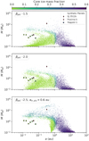 |
Fig. 13 Synthetic populations of planets calculated in single-embryo mode with reduced type I migration (fI : 0.1) as a function of a and M. The mass fraction of the summed-up ices is shown in color. The top panel shows the population of planets with a nominal planetesimal surface density slope βpls, whereas the other two panels have steeper planetesimal surface density slopes as indicated in the top left of the panel. The bottompanel displays the population of planets, where embryos and planetesimals are only placed outside of 0.6 au. |
4.2 Growth regimes
As shown in Sects. 3.1 and 3.3, the components that make up the planetary mass distribution (Fig. 10) are a population of very low-mass (~0.01 M⊕) “failed cores” at high semi-major axis and low-mass (~1 M⊕) planets mainly growing inside of the water iceline (“terrestrials”). In addition to these, the more massive planets (“horizontal branch” planets, M ~ 10 M⊕, Mordasini et al. 2009b), initially growing at larger separations and a few giant planets (M > 100 M⊕), populate the distribution.
In the following, the different origins of the sub-populations are addressed. In particular, we discuss the shape of the planetary-mass and the planet to star mass ratio distribution shown in Fig. 10.
The initial embryo mass of 0.01 M⊕ is large enough to lie in the oligarchic growth regime (Rafikov 2003; Ormel et al. 2010). At large separations, the oligarchic growth timescale becomes long. This leads to a population of planets that are not able to grow significantly and remain at large distances. These are excluded from our analysis using the cuts in period space. Despite the existence of failed cores at almost all of the sampled starting points and disk conditions, planets are able to grow and favorable conditions with short growth timescales are frequent outside the iceline. This allows for growth up to masses where type I migration becomes important. Therefore, migration could shape the mass distribution. To explore this scenario, weshow in Fig. 14 the population of planets as it is still growing with color-coded migration rates.
The distribution peaks at the planetary to stellar mass ratio of q ~ 1 × 10⁵. In this sub-population, planets from the “horizontal branch” as well as the “terrestrials” are the primary contributors and, apart from the giant planets, they stand as the most massive planets.
In principle, there could be three reasons for the mass distribution to drop at higher mass ratios than q ~ 1 × 10⁵, leading to a peaked shape: (1) the onset of rapid gas accretion could move planets quickly to larger masses, leading to the typical “desert” in the mass distribution (Ida & Lin 2004a); (2) the disk conditions and small isolation masses (Kokubo & Ida 2000) might not allow for further growth for planets growing close to the star, that is, for the “terrestrials”; or (3) fast type I migration could move the planets out of favorable growth regions, thus halting solid accretion.
The first point cannot be the main driver in our simulations because the number of planets that actually grow to become giant planets is too few to influence the shape of the mass distribution at lower masses. From Fig. 14, we can see mechanisms (2) and (3) at work: There is a clear decrease of planets in the inner systems at 1 Myr when going to larger masses. Although some more growth and collisions will occur at later times, the disk conditions are clearly limiting growth in the inner system. Additionally, we can identify planets colored in dark blue indicating fast type I migration that originate from the outer system that typically migrate inwards at ~5 M⊕ (q ~ 1.5 × 10⁻⁴) in the upper panel (0.1 M⊙), respectively, at ~20 M⊕ (q ~ 6 × 10⁻⁵) in the lower panel. The typical masses differ because, as discussed in Sect. 2.1, migration is a function of the stellar mass, disk mass, and planetary mass. Of particular importance is the mass at which the corotation torque saturates and planets rapidly drift inwards without time for further growth. This explains the different locations of the drop in the mass distribution of resulting planets. We note that, as the disk evolves, cools, and thins out, the typical onset of rapid type I migration is shifted to lower values. Therefore, the early snapshot of the first “fast migrators” at 1 Myr should give upper limits to the processes.
To summarize, we qualitatively identify that the saturation of corotation torques, as well as the growth-limits in the inner system, is shaping the planetary mass distribution below 50 M⊕. The non-linearity, despite a linear scaling of the disk mass, is likely due to the non-linear behavior of type I migration with disk mass via the temperature structure and the resulting scale heights.
At the upper end of the distribution lies a small fraction of planets which can overcome this type I migration barrier. Then, they undergo runaway gas accretion (Mizuno et al. 1978), reach the slower type II migration regime and become giants. A lot of solid mass is required to grow to the type II migration regime more quickly than type I migration timescales (~ 104 to ×105 yr).
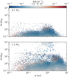 |
Fig. 14 Massand semi-major axes of the populations around 0.1 M⊙ and 1.0 M⊙ after 1 Myr of evolution. The normalized migration rate is colored and larger dots denote gap-opening planets that migrate in the type II regime. |
4.3 Frequency of Earths and super-Earths
After focusing on the origins of low-mass planets in our simulations, we discuss the same population of planets with regards to observations in this section. For planets with masses below ~100 M⊕, the best estimates on their frequency can be gained from transit surveys because of their large sample. Using the results from Kepler, Dressing & Charbonneau (2013) derive an occurrence of about one planet with orbital period shorter than 50 days and radii from 0.5 R⊕ to 4 R⊕ per cool star (T < 4000 K), while Gaidos et al. (2016) find around two planets per M dwarf with similar radii and orbital periods up to 180 days. From Fig. 12, it is apparent that more planets are formed in the synthetic simulations. This has already been reported in Mulders et al. (2019), who find a fraction of synthetic stars with planets that is five times greater compared to the Kepler sample. This finding still holds for lower-mass stars. The synthetic data on which their conclusion is based on, is very similar to the 1.0 M⊙ data set shown here.
Planet formation models do more readily yield planetary masses than radii, as gravity is the dominating force that is acting. Consequently, our results can more readily be compared to Pascucci et al. (2018) who use the Kepler sample to derive planetary and stellar masses. In contrast to this simple analysis, a future paper in this series will apply the technique described in the companion paper of Mishra et al. (2021) to use our computed planetary radii and derive a biased sample of planets to compare directly to Kepler.
Pascucci et al. (2018) find broken scaling relations in planet to star mass ratios obtained from Kepler and microlensing surveys, which can be discussed here without the compositional imprints on the radii. In the Kepler-based data of Pascucci et al. (2018), the position of the universal peak lies at M∕M⋆ = 2.8 × 10⁻⁵ indicated in the lower panel of Fig. 10. Our synthetic mass function does not show the same prominent peak, but a wider distribution of ratios (see Fig. 10). However, if more embryos would have started outside the iceline, a peak similar to the dash-dotted line in the upper panel of Fig. 10 should have been recovered at a location closer to the Pascucci et al. (2018) peak. In Fig. 10, we see that the distribution is not shifted exactly linearly with the stellar mass. Instead, a slight trend toward larger M∕M⋆ for lower stellar masses can be seen. In Pascucci et al. (2018), only the most massive F-stars do show a slightly lower mass ratio peak, while the peaks around G, K and M dwarfs lie at the same M∕M⋆. This could partially be due to a more narrow range of stellar masses that was available for their analysis.
Furthermore, the location of the peak at M∕M⋆ = 2.8 × 10⁻⁵ from Pascucci et al. (2018) is not perfectly matched by our models. Instead, the distributions drop at a value of M∕M⋆ which is a factor ~1.5 lower. This can either point toward migration in the models becoming too efficient at too low planetary masses, too low solid disk masses, or a preferred placement of the embryos could be influencing the results.
Based on these findings, we can conclude that if the mass distribution of planets indeed has a distinct peak and is not a remnant decrease of an inaccessible, broader distribution, then it is most likely due to type I migration halting growth. This pushes many planets of similar mass to the observable regime, which is expected to make up the bulk of the observed data. The planetary mass would then correspond to the mass where the positive corotation torques saturate. As can be seen in Fig. 1, it is lower for lower-mass stars, leading to a similar value in q. This would point toward more efficient embryo formation at larger distances and fewer “terrestrial-like” planet growth, which would be in line with works that propose that planetesimal formation preferably occurs outside the water iceline (Dra̧żkowska & Alibert 2017; Schoonenberg & Ormel 2017). Furthermore, it would strongly favor the migration mechanism in general compared to an in situ growth of planets. This pathway is an alternative to the scenario of pebble-based accretion models, where a peak in the mass distribution can be directly attributed to the pebble isolation mass (Liu et al. 2019).
4.4 Dependence of dynamical results on initial placement
Planetary orbital parameters, such as the eccentricity or the period ratio of neighboring planets are influenced by close encounters between them. The frequency of close encounters in turn depends sensitively on the initial placement of the synthetic embryos, since placing two embryos in close proximity to each other might lead to interactions already during the early growth stage when migration is still negligible.
One measure that can be used to quantify the probability of dynamical instabilities (i.e., gravitational interactions) is the mutual Hill radius of a pair of planets (Chambers et al. 1996)
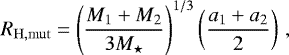 (4)
(4)
where M1, M2, a1, a2 are the masses and semi-major axes of two planets in a system. Typically, instabilities can occur if two planets are separated by less than ~3.5 mutual Hill radii (Chambers et al. 1996).
We chose the same initial embryo mass for all stellar masses. Thus, the distance, measured in mutual Hill radii, between the initially placed embryos in the simulations increases with increasing stellar mass. This means that in terms of dynamical interactions,the populations are not starting with the same initial conditions and thus, no strong conclusions should be drawn from the nominal populations with 50 embryos each.
This discussion touches the topic of the influence of the initial number of embryos, which is discussed in Paper II. There, it is shown that eccentricity and period ratio are quantities sensitive to the number of initial embryos that are placed in the disk. The scaling of the Hill radius  leads to a factor ~2 in the distance between initial embryos measured in mutual Hill radii between the 0.1 M⊙ population and the 1.0 M⊙ population. Coincidentally, a planetary population was calculated and presented in Paper II using 100 embryos around a 1.0 M⊙ star (Population NG76). We are therefore able to compare here the dynamical outcome between this population and the here presented 0.1 M⊙ case (NGM10), which have more similar initial dynamical conditions (see Fig. 15, dotted lines).
Due to growth and migration, the systems get more compact over time leading to lower mean distances measured in mutual Hill radii ( ) but, sporadically, the measure can increase if collisions or scattering of planets occur. The final states of the solar-type star population with 100 initial embryos and the 0.1 M⊙ population with 50 embryos are still quite close to each other. For comparison, the solar-type star population with 50 embryos has a mean over all systems around 27
  after starting at ~40. This is significantly different from the outcome with 100 embryos, which results in more closely packed systems with a mean over all systems of
  at ~20.
In Fig. 15, we can also see a slight trend to more packed systems for the population of planets around solar-type stars. Indeed, even though the initial  of the population of planets around solar-type stars is slightly larger than for the population around 0.1 M⊙, the resulting mean
  is lower. We argue that this is due to very little growth in some systems around 0.1 M⊙, which then leads to systems with mean
  closer to thehigher initial value. Although planets with arbitrary mass are included in Fig. 15, the same trends are recovered if small mass planets are removed. Thus, it is relevant for observable planets.
Having established a closer dynamical relationship between the population with 50 embryos around a 0.1 M⊙ (NGM10) star and the one with 100 embryos around 1.0 M⊙ (NG76), we can compare the dynamical evolution of the systems of those two populations. Figure 16 shows the period ratio of neighboring planets of any mass and semi-major axis that formed in NG76 (blue line) and NGM10 (brown). An apparent difference is the number of planets in or close to mean-motion resonances seen as vertical jumps of the lines in Fig. 16. The total number of planet pairs with both P1, P2 < 300 d and M1, M2 > 0.1 M⊕ close to integer period ratios (within 2%) is 35.5% of the planets in the 0.1 M⊙ population compared to 27.8% in NG76. This trend would not have been recovered if we compared the 0.1 M⊙ population NGM10 to the 1.0 M⊙ one (NG75) with also 50 initial embryos but an initially larger separation between them measured in mutual Hill radii. There, in NG75, a larger number of planet pairs is close to mean-motion resonances (47.0%) than in NGM10. The trend of fewer planets close to mean-motion resonances with increasing number of embryos was already found by Alibert et al. (2013) by comparing simulations with up to 20 embryos and more recently Mulders et al. (2019) discuss the period ratio distribution of synthetic planets compared to observed systems.
An interesting aspect of the mean-motion resonant chains is that there are a few planet pairs in second-order mean-motion resonance. Second order resonances are less frequently produced in non-eccentric systems and need to be more dynamically excited thanwhat results from low-eccentricity type I migration into resonant chains (see e.g. Coleman et al. 2019). In our simulations, a difference between the stellar masses is already present at the end of the disk lifetime: The 0.1 M⊙ population includes 133 (2.8%) pairs close to 5:3 period ratios with P1, P2 < 300 and M1, M2 > 0.1 M⊕ whereas there are 149 (1.6%) such pairs in the 1.0 M⊙ population at this early time. With the disappearance of the damping gas, a reduction in the number of systems in mean-motion resonances occurs (Izidoro et al. 2017) and the numbers go down to 78 (2.1%) and 91 (2.3%) for 0.1 M⊙ and 1.0 M⊙ respectively. In this context, we recall that the TRAPPIST-1 system planets d and c are close to 5:3 mean-motion resonance, which is rare in the simulations (3.8% of the pairs for planet pairs with masses larger than 0.1 M⊕ and semi-major axes smaller than 0.1 au). Because there are only upper limits on the occurrence rates of systems similar to TRAPPIST-1 available (Sestovic & Demory 2020), it is not yet possible to conclude if our simulated results concerning mean-motion resonances for very-low-mass stars agree with observations.
Figure 16 additionally shows the observed Kepler multi-planetary systems period ratio for reference. We note that the simple cut in masses at 0.1 M⊕ and periods at 300 days that we apply for the synthetic systems is not very well suited for the comparison of the period ratios to the observed systems. Some planetary pairs that are more distant from the star compared to the observed population are included in the synthetic data. Applying the realistic bias from Kepler will be addressed in a future study (using the technique of the companion paper Mishra et al. 2021).
The last dynamical property we discuss in this work is the eccentricity of the planetary orbits. Similarly to the discussion above, we can also attribute a large part of a decreasing eccentricity trend with stellar mass in the nominalpopulation to the initial conditions. Indeed, Fig. 17 shows the nominal 0.1 and 1.0 M⊙ populations with 50 embryos each (NGM10, NG75), but additionally the population with 100 embryos (NG76). It is apparent that increasing the number of embryos increases the eccentricity, which is due to an initially closer setting. Reducing the stellar mass while keeping the number of embryos fixed and at the same mass, had a similar effect. Comparing NG76 and NGM10 again, only small differences in eccentricities can be found, with a few highly eccentric planets around solar mass stars that are not present in NGM10. This can be attributed to the systems with giant planets, where the orbits of the smaller planets in the same system can become very eccentric.
Overall, the eccentricity distribution is more sensitive to the initial placement than other parameters. In contrast, it is quite insensitive with regard to the mass of the host star (see also Table 5) as long as the initial separation stays similar.
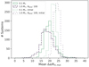 |
Fig. 15 Mean distance between all neighboring planets in a system measured in mutual Hill radii (Chambers et al. 1996). The initial placement corresponds to the dotted lines and the resulting values are shown using a solid line. The number of injected embryos for the population of planets around 0.1 M⊙ stars is 50, whereas we insert 100 embryos for this population of planets around 1.0 M⊙ stars. |
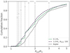 |
Fig. 16 Orbital period ratio of all neighboring planets including planets with M > 0.1 M⊙ and periods P < 300 days. Two synthetic populations of planets are shown: one around a solar-type star with initially 100 embryos (NG76) and one around stars with a mass of 0.1 M⊙ (NGM10). The Kepler multi-planetary system period ratios are displayed for reference (NASA Exoplanet Archive, accessed 9.12.2019). |
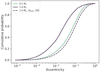 |
Fig. 17 Cumulative distribution function of the planetary eccentricities for synthetic populations NGM10 (0.1 M⊙, 50 embryos, green), NG75 (1.0 M⊙, 50 embryos, dark blue, solid), and NG76 (1.0 M⊙, 100 embryos, dashed, dark blue). Only planets with masses above 0.1 M⊕ are included. |
4.5 Solid mass reservoirs
Planetesimal accretion is a process regulated by the eccentricities and inclinations of the planetesimals in the proximity of the growing protoplanet (Ida & Makino 1992a,b; Inaba et al. 2001; Fortier et al. 2013). For larger planetesimal eccentricities and inclinations,lower accretion rates result and if the planet becomes massive enough, we find that it can even eject a significant amount of planetesimals completely from the system. The region for which one protoplanet perturbs the planetesimal disk expands to a few tens of Hill radii. Therefore, indirect growth reduction for the less massive embryos in this region occurs. This is in line with the findings of Alibert et al. (2013). One technical difference is that in this third generation of the model, the planetesimal surface density inside a feeding zone shared by several planets is calculated differently. It is not set to the mean value calculated over the whole zone but only to the mean value over the part attributed to one growing embryo (see Paper I). This is different from the treatment in Alibert et al. (2013), where the former mean over the whole merged feeding zone was used. For the models presented here, this leads to a lesser extent of mass transport to the inner regions where planetesimals can be more easily accreted. Nevertheless, the results for both approaches are similar.
For an individual embryo, growth by solid accretion to masses above the classical isolation mass (Lissauer & Stewart 1993) is commonly possible due to migration to non-depleted regions. In addition to the competition for and excitation of planetesimals, this makes an analytic treatment of solid accretion even more difficult. Therefore, we investigate the ratio of the sum of the solids in planetarycores to the solids initially inserted into the planetesimal disk of a system (Fig. 18). We term this the efficiency of solid accretion.
In Fig. 18, a tail toward very low efficiencies is found in the population around a 1.0 M⊙ star, which can be attributed to systems with at least one giant planet (dotted line). The overall bulk of the distribution without giant planets peaks at a similar location in the two populations. The reason for the lower apparent efficiency for the systems with a giant planet is mainly ejection of planetary embryos (see also Schlecker et al. 2021). In NG76 ejection of planets occurred in 219 systems. The mean mass of ejected planets was 46.7 M⊕ per system with ejection. In contrast to that, in NGM10 ejection of planets occurred in only 38 systems with a mean mass of ejected planets of 0.27 M⊕, which is lessrelative to the initial mass of solids.
From these results, we can qualitatively expect that free-floating planets (e.g., Sumi et al. 2011) predominantly originate from systems around stars of higher mass with more massive disks if they are mainly produced by planet-planet scattering (see, e.g., Veras & Raymond 2012 and Stock et al. 2020 for discussions on their formation). The dependency on stellar mass is not linear due to gas accretion: systems with giant planets that underwent rapid gas accretion eject much more planetary mass to interstellar space than systems where no significant gas accretion occurred. Additionally, we find the bulk of the ejected mass to be in the form of embryos and not in the form of ejected planetesimals2. This finding is again a function of the number, spacing, and mass of the initially placed embryos and should be addressed in detail in future works.
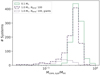 |
Fig. 18 Fraction of final solid mass content in planets in a system divided by the initial solid mass in the planetesimal disk. The light green line corresponds to the population around a 0.1 M⊙ star with 50 embryos (NGM10) and the dashed, dark blue line to the population around a 1.0 M⊙ star with 100 initial embryos (NG76). The dotted histogram shows the same quantity for the systems with at least one existing giant planet (M > 100 M⊕) in NG76. |
4.6 The case of TRAPPIST-1
The population of synthetic planets around an 0.1 M⊙ star (NGM10) is well suited for comparison to the TRAPPIST-1 system (Gillon et al. 2016, 2017). TRAPPIST-1 is an ultra-cool dwarf star with an estimated mass of 0.089 ± 0.006M⊙ (Grootel et al. 2018). The system is unique due to the high number of detected transiting planets and their mass constraints (Grimm et al. 2018; Agol et al. 2021). Thus, TRAPPIST-1 provides a unique opportunity to benchmark planet formation models against (see also Ormel et al. 2017; Alibert & Benz 2017; Coleman et al. 2019; Schoonenberg et al. 2019; Miguel et al. 2020).
The TTV fits for the TRAPPIST-1 system exclude additional planets with significant mass for at least the region within 0.1 au (Grimm et al. 2018). Therefore, it makes sense to investigate the properties of the synthetic planets with masses above 0.1 M⊕ within 0.1 au (here dubbed the TRAPPIST-1 region) in the synthetic 0.1 M⊙ population NGM10 and compare them with what we know for the TRAPPIST-1 planets.
4.6.1 Example systems
As a first pathway to explore systems similar to TRAPPIST-1, we show a selection in Fig. 19. The systems were chosen based on the smallest differences in total mass in the TRAPPIST-1 region (see Sect. 4.6.3). Even though the total mass incorporated in the region is similar in all these example systems, very different patterns are visible.
The initial solid mass is not distributed evenly in the initial systems. Our chosen slope of βs = −1.5 results in isolation masses that increase with semi-major axis with a slope of 0.5. This could still be visible in the final systems despite the simple arguments that are used to calculate the planetesimal isolation mass (Kokubo & Ida 2000). Whereas in the lower three panels of Fig. 19, there are hints of an increasing mass gradient with semi-major axis, no such trend can be recognized in simulation 11 and in the TRAPPIST-1 system itself. While not always the case, simulation 11 is an example that collisions and migration can erase the memory of the initial solid mass content at the starting location of the embryos.
The number of planets in the region differs significantly between the systems; simulation 11 and 787 are with seven and six planets close to the seven observed planets. In contrast, simulation 673 produced an astonishing 11 planets in the same region. Due to the short orbital periods, it is unlikely that the 20 Myr of numerical N-body integration is not sufficient to reveal if that system is dynamically unstable. Therefore, such systems are at least theoretically possible. It is not clear what distinguishes simulation 673 from the other systems. The inner edge of the disk lies at 0.29 au compared to 0.24 au, 0.012 au, and 0.36 au for simulations 11, 787, and 977 respectively. It might just be a coincidence that a last series of collisions due to a system-wide instability did not occur in simulation 673; thus, a large number of planets was retained.
A common occurrence are more ice-rich planets outside the observable region. As embryos are assumed to have the capacity to form everywhere in the disk, this is expected and should be interpreted with this assumption in mind. We also note that all these systems have undergone collisions between embryos in the inner system. In our simulations, these collisions lead to perfect merging, but in reality, fragmentation would occur and typically decrease the resulting planetary mass and enhance the compositional diversity (Emsenhuber et al. 2020).
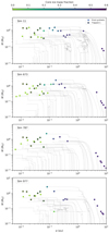 |
Fig. 19 Synthetic systems with final planetary masses most similar to the Trappist-1 system. The mass difference to the observed masses (Agol et al. 2021) are −0.17 M⊕, 0.14 M⊕, −0.15 M⊕, and 0.00 M⊕. Thin lines denote the evolution over time of individual planets. If they stop without ending in a colored dot, the corresponding embryo was ejected or accreted by a more massive planet. Despite closely matching in total mass, significant differences between systems are visible. |
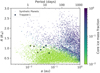 |
Fig. 20 Orbital distance, planetary radius diagram of synthetic planets around a 0.1 M⊙ star. For comparison, the Trappist-1 system (Agol et al. 2021) and the subsample of synthetic planets around them is shown. The core ice mass fraction is here colored using a logarithmic scale for better visibility of the low values derived assuming a core iron mass fraction of 32.5% in Trappist-1. |
4.6.2 Statistics of synthetic planets inside 0.1 au
In our model results, consisting of a total of 1000 systems, typically only a few planets grow to 0.1 M⊕ masses. The most common number of planets in the TRAPPIST-1 region (M > 0.1 M⊕, a < 0.1 au) is 1, which occurs in 330 systems. In 182 systems, not a single planet is in the TRAPPIST-1 region and only 20% of the systems do have more than three planets there. This low number is mainly due to little growth in many systems and further reduced by evolutionary paths that led to a single massive close-in planet that accreted all the other embryos. This second scenario is common in disks with an above-average initial solid mass and supported by fast type I migration. If the migration speed was reduced, for example by a lower viscous α or due to wind-driven accretion (Ogihara et al. 2018), there would be fewer systems where the growing embryos are forced by strong disk torques into each others proximity, which then leads to fewer close encounters and collisions.
Figure 20 shows the population of planets in NGM10 in semi-major axis, radius space. The zoom into the region where the TRAPPIST-1 planets lie reveals more clearly that the density of synthetic planets drops toward the star as inner edges of disks become comparable to the location of TRAPPIST-1 b. Additionally, in terms of rocky planets, the TRAPPIST-1 planets populate the parameter space of the largest such bodies. This is consistent with the observational bias as transit surveys are most sensitive to the largest planets.
Moving on to the statistics of compositions, the ice mass fraction in the cores of synthetic planets in the TRAPPIST-1 zone are shown in Fig. 21. Currently, the TRAPPIST-1 planets are considered to be quite rocky (Dorn et al. 2018; Grimm et al. 2018), even more so in the recent results of Agol et al. (2021), who find ice mass fractions below 1% for low-iron core masses (18%), below 7% for Earth-like core mass fractions (32.5%), and still below 14% for large iron cores (50%).
Additionally, Agol et al. (2021) find for the updated masses that the ice mass fraction increases with orbital period within error bars throughout the whole TRAPPIST-1 system. This is in much better agreement with theoretical results compared to previous derived compositions (Dorn et al. 2018). Such an outcome is expected from classical planet formation theory and in agreement with the Solar System.
One aspect that is less intuitive is the prevalence of more ice-rich planets with increasing mass due to planetary migration (the “horizontal branch” in Fig. 7, see also Sect. 3.1 and Ida & Lin 2005; Mordasini et al. 2009a; Alibert et al. 2011; Alibert & Benz 2017). From the data in Agol et al. (2021), it is not yet clear if an increase in the ice massfraction with planetary mass is also present in the TRAPPIST-1 system. One indication could come from the lower inferred ice mass fraction for the outermost planet h compared to its neighbor g. However, the uncertainties are much too large to confirm the trend of larger ice mass fractions for planets with masses above 1 M⊕, which we show in Fig. 7.
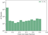 |
Fig. 21 Histogram of the core ice mass fractions of the 2222 synthetic planets in the TRAPPIST-1 region (M > 0.1 M⊕, a < 0.1 au). The shown population of synthetic planets is calculated around a 0.1 M⊙ star with 50embryos (NGM10). Most planets are purely rocky, but 314 (14%) show ice fractions larger than 0.1. |
4.6.3 Initial condition regime
To compare the simulated systems with TRAPPIST-1, we chose to take the number Np and the difference to TRAPPIST-1 in total mass ΔMtotal (where Mtotal of TRAPPIST-1 is 6.45± 0.10M⊕, Agol et al. 2021). For both, we only take planets with masses M > 0.1 M⊕ and semi-major axes a < 0.1 au into account. This simple approach is a first exploration of the similarity of TRAPPIST-1 and the synthetic data in terms of the most fundamental parameters. A more complex similarity criterion of systems will be applied in future works following Alibert (2019). The colors of Figs. 22 and 23 display Np and ΔMtotal, where one point corresponds to a synthetic system. It is interesting to show them as a function of the initial solid mass and the inner disk edge to determine the most likely initial parameters of the disk from which the TRAPPIST-1 planets formed. For both, Np and ΔMtotal, there is a clear correlation with the initial solid mass, whereas it is only for the number of planets that there seems to be a correlation with the inner disk edge.
For ΔMtotal, this can be explained by the mass transport via type I migration. The migration rates and thus the solid mass flux to the inner regionis independent of the inner disk edge. Thus, a similar fraction of the total solid mass in the disk is transported inside 0.1 au in all disks. The initial mass in planetesimals inside 0.1 au only varies negligibly with the inner edge.
However, this mass can be distributed very differently to the planets. In a number of disks at the high-end tail of the solid masses (Msolid > 60 M⊕), there are only one to four oligarchs that grew by accreting the rest of the embryos. Due to the higher initial solid mass, largerplanets form which correspondingly have bigger Hill spheres and interact more often gravitationally with the other embryos. Consequently, they can be ejected or accreted by other planets, where both outcomes lead to a smaller number of planets in a given zone. Therefore, Fig. 22 shows a peak in Np inside the TRAPPIST-1 zone which is located at moderate, but above-average disk solid masses (10 M⊕ < Msolid < 60 M⊕). At lower than average disk solid masses, the number of planets decreases. This is due to planets not growing to masses above 0.1 M⊕. Thus, they are not identified to lie in the TRAPPIST-1 zone and additionally, very little transport of solid material due to type I migration takes place.
Overall, one sweet-spot for the formation of a system with a similar amount of planetary mass at comparable semi-major axes as TRAPPIST-1 can be located at 30 M⊕≲ Msolid ≲ 50 M⊕, which coincides with the region where seven planets inside 0.1 au are frequently present given an inner disk edge below at least 0.06 au. These values are larger than the nominal values of 13.3 M⊕ and 18.3 M⊕, respectively,applied in the models of Ormel et al. (2017) and Schoonenberg et al. (2019).
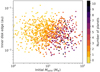 |
Fig. 22 Disk initial conditions color-coded by multiplicity. We plot only the planets in the TRAPPIST-1 region, i.e., with semi-major axis less than 0.1 au and mass larger than 0.1 M⊕. |
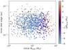 |
Fig. 23 Disk initial conditions color-coded by difference of total mass to the TRAPPIST-1 system. Individual planet masses are only included if their semi-major axis is less than 0.1 au and their mass is larger than 0.1 M⊕. Systemswith no planets lying in this regime are drawn as empty black circles. The darkest points show systems most TRAPPIST-1 similar at around 30 M⊕ of initial solid mass. |
4.7 Comparison with previous works
We now briefly discuss our results in context of other theoretical works. As there are a number of works focusing on ultra-late M dwarfs of 0.01 M⊙, this will be the focus of the comparison. In Sect. 4.1, we covered the other major branch of works focusing on giant planet formation.
We predominantly find a large rocky population of planets making up about 90% of the planets and a smaller, more massive, water-bearing population in the TRAPPIST-1 region (see Fig. 21). This is due to a large amount of accretion inside the water iceline, similarly to what is found in Schoonenberg et al. (2019) but in contrast to the findings of Alibert & Benz (2017), Miguel et al. (2020), and Coleman et al. (2019) who find mostly water-rich planets. Coleman et al. (2019) assumed an insignificant amount of rocky planetesimals initially, while Miguel et al. (2020) have computed a snowline that lies much closer to the star than in our work. This is due to the differing disk temperature calculations: To estimate disk temperatures, Miguel et al. (2020) use gas accretion rates Ṁacc on the order of 10−10 M⊙ yr−1, which corresponds to a later, cooler stage in the disk evolution compared to our assumed planetesimal formation at the beginning of our simulations (where Ṁacc ≃ 10−9 M⊙ yr−1). Additionally, the disks presented here are assumed to be twice as turbulent (α = 2 × 10⁻³) compared to the disks in Miguel et al. (2020) (α = 1 × 10⁻³) leading to hotter disks. For these two reasons, Miguel et al. (2020) start their simulation with much fewer rocky planetesimals in comparison to our simulations.
The best correlation with our model can be found in the work of Alibert & Benz (2017). Our results differ from theirs for three different reasons: (1) Alibert & Benz (2017) found that for more massive disks, more rocky planets appear, and they scale the disk mass to the power of 1.2 with the stellar mass. Their “heavy” disk case lies closer to our mass distribution and already produces ~20% rocky planets. (2) We ran simulations with 50 embryos, compared to Alibert & Benz (2017), who ran their simulations with 10 embryos. More embryos lead to more potential accretion close to the star, since the sum of all feeding zone increases, which is the limiting factor for growth in the inner region in the initial stages. (3) The slope of the planetesimal surface density differs in the two simulations. While we use a slope of βpls = −1.5, Alibert & Benz (2017) used a shallower slope of −0.9. Therefore, by construction, more rocky material is available in our new set of simulations. This third point is an additional relevant difference to the work of Miguel et al. (2020). Current planetesimal formation models favor steeper slopes, but potentially lower planetesimal formation within the water iceline (Dra̧żkowska & Alibert 2017; Lenz et al. 2019; Voelkel et al. 2020).
As of now, no clear conclusion should be drawn concerning the validity of the pathway of rocky planet formation by almost in situ accretion, which has been seen to be dominant in our work. Due to the moving water iceline, the resulting planetary composition is a strong function of the location and timing of planetesimal formation. This will be incorporated in our model following Voelkel et al. (2020) in the future. For now, we show that if enough planetesimals are assumed to have formed within the water iceline, rocky planets will form directly consistent with the TRAPPIST-1 planets. Otherwise, to reproduce the observed population of rocky planets, the planetesimals or the planets have to desiccate by some additional process (e.g., due to radioactive heating of planetesimals as in Lichtenberg et al. 2019 or by ablation of pebbles in the planetary envelopes as discussed by Coleman et al. 2019).
5 Summary and conclusions
In this part of the New Generation Planetary Population Synthesis (NGPPS) series, we employed the Generation III Bern model of planet formation and evolution, introduced in Paper I, to explore the influence of the stellar mass. We calculated ~1000 synthetic multi-planet systems for a grid of stellar masses (0.1 M⊙, 0.3 M⊙, 0.5 M⊙, 0.7 M⊙, and 1.0 M⊙) and with an initial 50 planetary embryos per system. While we linearly scaled the gas and solid disk mass with stellar mass, we assumed physical disk boundaries constant in orbital period and kept the disk lifetime fixed.
This yields a data set for which we found:
-
A larger number of giant planets with larger stellar mass. In particular, no giant planets formed for M⋆ < 0.5 M⊙.
-
The most frequent temperate (potentially habitable) planet host to be M dwarfs with masses of 0.3 M⊙–0.5 M⊙. Additionally, we find a strong metallicity dependence of the temperate planet occurrence rate at low stellar masses. Therefore, planet searches aiming for temperate, terrestrial planets around low-mass stars should target metal-rich objects.
-
The planetary mass function does not shift in a strictly linear fashion with the stellar mass despite the linear scaling of the gas and solid disk mass. This is due to more ejected planets for higher stellar masses because of the growth of giant planets.
-
As consequences of the previous point, there is a reduced apparent efficiency of solid accretion toward higher stellar mass due to ejection of planetary embryos. Directly related to this, we find that planets ejected by planet-planet scattering originate from stars with masses of at least a solar mass.
-
A strong dependency of the dynamical properties such as period ratios and eccentricities on the initial proximity of the embryos measured in mutual Hill radii (initial spacing). Using this measurement, the systems are more compact for higher stellar masses at the end of the simulations.
-
A high occurrence of mean-motion resonances due to migration, which is in contrast to the lower number of observed resonant multi-planetary systems. For a similar initial spacing, ~10 % more pairs within 300 d orbital periods are in resonance around ultra-late M-dwarfs compared to solar-like stars.
-
A sweet spot in terms of initial solid mass content (30 to 50 M⊕) and inner disk edge (closer than 0.06 au) to get a system like TRAPPIST-1, as measured by the observable mass.
-
A clear predominance of rocky compositions for planets in the innermost 0.1 au of low-mass stars due to enhanced rocky planetesimal accretion. This is a strong function of how many planetesimals and embryos were initially placed closer to the star than the water iceline.
-
A pathway for the formation of giant planets around very low-mass stars via core accretion: While it is sufficient to reduce type I migration, even more giants form if planetesimals are initially more concentrated toward the star.
Despite the advancements in recent years, there are a number of limitations to the model. Due to computational cost, it was not possible to study the influence of different model parameters (e.g., the viscous α parameter, planetesimal size, or envelope opacity) or initial condition scalings (like the disk mass). Of particular importance is the assumed planetesimal size of 600 m in diameter, which is at odds with planetesimal formation predictions (Johansen et al. 2012; Li et al. 2019; Klahr & Schreiber 2021). However, in the Kuiper Belt, there could have existed a numerous population of smaller planetesimals (Schlichting et al. 2013; Kenyon & Bromley 2020, see also Arimatsu et al. 2019; Morbidelli et al. 2021). We expect that for all stellar masses, an increase in the planetesimal size would increase the solid accretion timescale and thus decrease the number and mean mass of the planets (Fortier et al. 2013). Similarly, larger dust opacities in the planetary envelopes slow down cooling and thus gas accretion (Mordasini 2014). We also see considerable potential for improvement in the treatment of the equation of state for water (Haldemann et al. 2020) which influences the radius distribution, the formation location of embryos and planetesimals (Voelkel et al. 2020, 2021), and the accretion of pebbles (Brügger et al. 2018, 2020).
Keepingin mind these limitations, our analysis quantifies, global trends in multiplanet systems as a function of stellar mass, which have previously been studied only in models with a narrower focus. A major benefit to this work is the availability of enough statistical data and the ability to make use of global simulations of planetary systems to find these aspects in a single, coherent theoretical framework. The results compare reasonably well to de-biased observational data where available. In the future, these comparisons should be examined in greater detail.
Acknowledgements
Parts of this work have been carried out within the frame of the National Centre for Competence in Research PlanetS funded by the Swiss National Science Foundation (SNSF). R.B. and Y.A. acknowledge the financial support from the SNSF under grant 200020_172746. This work was supported by the DFG Research Unit FOR2544 “Blue Planets around Red Stars”, project no. RE 2694/4-1. A.E. acknowledges the support from The University of Arizona. A.E. and C.M. acknowledge the support from the SNSF under grant BSSGI0_155816 “PlanetsInTime”. This research has made use of the NASA Exoplanet Archive, which is operated by the California Institute of Technology, under contract with the National Aeronautics and Space Administration under the Exoplanet Exploration Program. The plots shown in this work were generated using matplotlib (Hunter 2007) and seaborn (https://seaborn.pydata.org/index.html).
References
- Adachi, I., Hayashi, C., & Nakazawa, K. 1976, Prog. Theor. Phys., 56, 1756 [CrossRef] [Google Scholar]
- Adams, F. C., Hollenbach, D., Laughlin, G., & Gorti, U. 2004, ApJ, 611, 360 [NASA ADS] [CrossRef] [Google Scholar]
- Affer, L., Micela, G., Favata, F., Flaccomio, E., & Bouvier, J. 2013, MNRAS, 430, 1433 [Google Scholar]
- Agol, E., Dorn, C., Grimm, S. L., et al. 2021, Planet. Sci. J., 2, 1 [NASA ADS] [CrossRef] [Google Scholar]
- Alcalá, J. M., Manara, C. F., Natta, A., et al. 2017, A&A, 600, A20 [NASA ADS] [CrossRef] [EDP Sciences] [Google Scholar]
- Alessi, M., Pudritz, R. E., & Cridland, A. J. 2020, MNRAS, 493, 1013 [NASA ADS] [CrossRef] [Google Scholar]
- Alexander, R., Pascucci, I., Andrews, S. M., Armitage, P., & Cieza, L. 2014, in Protostars and Planets VI, eds. H. Beuther, R. S. Klessen, C. P. Dullemond, & T. Henning (Tucson: University of Arizona Press), 475 [Google Scholar]
- Alibert, Y. 2019, A&A, 624, A45 [NASA ADS] [CrossRef] [EDP Sciences] [Google Scholar]
- Alibert, Y., & Benz, W. 2017, A&A, 598, L5 [NASA ADS] [CrossRef] [EDP Sciences] [Google Scholar]
- Alibert, Y., Mordasini, C., & Benz, W. 2004, A&A, 417, L25 [NASA ADS] [CrossRef] [EDP Sciences] [Google Scholar]
- Alibert, Y., Mordasini, C., Benz, W., & Winisdoerffer, C. 2005, A&A, 434, 343 [NASA ADS] [CrossRef] [EDP Sciences] [Google Scholar]
- Alibert, Y., Mordasini, C., & Benz, W. 2011, A&A, 526, A63 [NASA ADS] [CrossRef] [EDP Sciences] [Google Scholar]
- Alibert, Y., Carron, F., Fortier, A., et al. 2013, A&A, 558, A109 [NASA ADS] [CrossRef] [EDP Sciences] [Google Scholar]
- Andrews, S. M., Wilner, D. J., Hughes, A. M., Qi, C., & Dullemond, C. P. 2010, ApJ, 723, 1241 [Google Scholar]
- Andrews, S. M., Rosenfeld, K. A., Kraus, A. L., & Wilner, D. J. 2013, ApJ, 771, 129 [Google Scholar]
- Andrews, S. M., Terrell, M., Tripathi, A., et al. 2018, ApJ, 865, 157 [Google Scholar]
- Anglada-Escudé, G., Boss, A. P., Weinberger, A. J., et al. 2012, ApJ, 746, 37 [Google Scholar]
- Anglada-Escudé, G., Amado, P. J., Barnes, J., et al. 2016, Nature, 536, 437 [Google Scholar]
- Ansdell, M., Williams, J. P., Manara, C. F., et al. 2017, AJ, 153, 240 [Google Scholar]
- Ansdell, M., Williams, J. P., Trapman, L., et al. 2018, ApJ, 859, 21 [NASA ADS] [CrossRef] [Google Scholar]
- Arimatsu, K., Tsumura, K., Usui, F., et al. 2019, Nat. Astron., 3, 301 [NASA ADS] [CrossRef] [Google Scholar]
- Artigau, É., Gagné, J., Faherty, J., et al. 2015, ApJ, 806, 254 [NASA ADS] [CrossRef] [Google Scholar]
- Baraffe, I., Homeier, D., Allard, F., & Chabrier, G. 2015, A&A, 577, A42 [NASA ADS] [CrossRef] [EDP Sciences] [Google Scholar]
- Barenfeld, S. A., Carpenter, J. M., Ricci, L., & Isella, A. 2016, ApJ, 827, 142 [Google Scholar]
- Bate, M. R. 2012, MNRAS, 419, 3115 [NASA ADS] [CrossRef] [Google Scholar]
- Bell, K. R., & Lin, D. N. C. 1994, ApJ, 427, 987 [NASA ADS] [CrossRef] [Google Scholar]
- Benítez-Llambay, P., Masset, F., & Beaugé, C. 2011, A&A, 528, A2 [NASA ADS] [CrossRef] [EDP Sciences] [Google Scholar]
- Benz, W., Ida, S., Alibert, Y., Lin, D. N. C., & Mordasini, C. 2014, in Protostars and Planets VI, eds. H. Beuther, R. S. Klessen, C. P. Dullemond, & T. Henning (Tucson: University of Arizona Press), 697 [Google Scholar]
- Bodenheimer, P., & Pollack, J. B. 1986, Icarus, 67, 391 [Google Scholar]
- Bonfils, X., Forveille, T., Delfosse, X., et al. 2005, A&A, 443, L15 [NASA ADS] [CrossRef] [EDP Sciences] [Google Scholar]
- Bonfils, X., Almenara, J.-M., Cloutier, R., et al. 2018, A&A, 618, A142 [NASA ADS] [CrossRef] [EDP Sciences] [Google Scholar]
- Boss, A. P. 1997, Science, 276, 1836 [Google Scholar]
- Bouchet, J., Mazevet, S., Morard, G., Guyot, F., & Musella, R. 2013, Phys. Rev. B, 87, 094102 [Google Scholar]
- Bouchy, F., Doyon, R., Artigau, É., et al. 2017, The Messenger, 169, 21 [NASA ADS] [Google Scholar]
- Bouvier, J., Alencar, S. H. P., Harries, T. J., Johns-Krull, C. M., & Romanova, M. M. 2007, in Protostars and Planets V, eds. B. Reipurth, D. Jewitt, & K. Keil (Tucson: University of Arizona Press), 479 [Google Scholar]
- Brügger, N., Alibert, Y., Ataiee, S., & Benz, W. 2018, A&A, 619, A174 [Google Scholar]
- Brügger, N., Burn, R., Coleman, G. A. L., Alibert, Y., & Benz, W. 2020, A&A, 640, A21 [NASA ADS] [CrossRef] [EDP Sciences] [Google Scholar]
- Bryson, S., Kunimoto, M., Kopparapu, R. K., et al. 2021, AJ, 161, 36 [NASA ADS] [CrossRef] [Google Scholar]
- Burdanov, A., Delrez, L., Gillon, M., & Jehin, E. 2018, in Handbook of Exoplanets, eds. H. J. Deeg, & J. A. Belmonte (Cham: Springer International Publishing), 1 [Google Scholar]
- Butler, R. P., Johnson, J. A., Marcy, G. W., et al. 2006, PASP, 118, 1685 [Google Scholar]
- Cameron, A. G. 1978, Moon the Planets, 18, 5 [NASA ADS] [CrossRef] [Google Scholar]
- Chambers, J. E. 1999, MNRAS, 304, 793 [Google Scholar]
- Chambers, J. E. 2006, Icarus, 180, 496 [NASA ADS] [CrossRef] [Google Scholar]
- Chambers, J., Wetherill, G., & Boss, A. 1996, Icarus, 119, 261 [NASA ADS] [CrossRef] [Google Scholar]
- Choi, J., Dotter, A., Conroy, C., et al. 2016, ApJ, 823, 102 [Google Scholar]
- Clarke, C. J., Gendrin, A., & Sotomayor, M. 2001, MNRAS, 328, 485 [NASA ADS] [CrossRef] [Google Scholar]
- Coleman, G. A. L., & Nelson, R. P. 2014, MNRAS, 445, 479 [Google Scholar]
- Coleman, G. A. L., & Nelson, R. P. 2016, MNRAS, 460, 2779 [NASA ADS] [CrossRef] [Google Scholar]
- Coleman, G. A. L., Leleu, A., Alibert, Y., & Benz, W. 2019, A&A, 631, A7 [NASA ADS] [CrossRef] [EDP Sciences] [Google Scholar]
- Crida, A., Morbidelli, A., & Masset, F. 2006, Icarus, 181, 587 [Google Scholar]
- Delfosse, X., Forveille, T., Mayor, M., et al. 1998, A&A, 338, L67 [Google Scholar]
- Delrez, L., Gillon, M., Queloz, D., et al. 2018, SPIE Conf. Ser., 10700, 107001I [Google Scholar]
- Demory, B.-O., Pozuelos, F. J., Gómez Maqueo Chew, Y., et al. 2020, A&A, 642, A49 [NASA ADS] [CrossRef] [EDP Sciences] [Google Scholar]
- Dittkrist, K.-M. K.-M., Mordasini, C., Klahr, H., Alibert, Y., & Henning, T. 2014, A&A, 567, A121 [NASA ADS] [CrossRef] [EDP Sciences] [Google Scholar]
- Dorn, C., Khan, A., Heng, K., et al. 2015, A&A, 577, A83 [NASA ADS] [CrossRef] [EDP Sciences] [Google Scholar]
- Dorn, C., Mosegaard, K., Grimm, S. L., & Alibert, Y. 2018, ApJ, 865, 20 [NASA ADS] [CrossRef] [Google Scholar]
- Dra̧żkowska, J., & Alibert, Y. 2017, A&A, 608, A92 [CrossRef] [EDP Sciences] [Google Scholar]
- Dra̧żkowska, J., Alibert, Y., & Moore, B. 2016, A&A, 594, A105 [CrossRef] [EDP Sciences] [Google Scholar]
- Dressing, C. D., & Charbonneau, D. 2013, ApJ, 767, 95 [Google Scholar]
- Dressing, C. D., & Charbonneau, D. 2015, ApJ, 807, 45 [Google Scholar]
- Emsenhuber, A., Cambioni, S., Asphaug, E., et al. 2020, ApJ, 891, 6 [NASA ADS] [CrossRef] [Google Scholar]
- Emsenhuber, A., Mordasini, C., Burn, R., et al. 2021a, A&A, 656, A69 (Paper I) [NASA ADS] [CrossRef] [EDP Sciences] [Google Scholar]
- Emsenhuber, A., Mordasini, C., Burn, R., et al. 2021b, A&A, 656, A70 (Paper II) [NASA ADS] [CrossRef] [EDP Sciences] [Google Scholar]
- Endl, M., Cochran, W. D., Kuerster, M., et al. 2006, ApJ, 649, 436 [NASA ADS] [CrossRef] [Google Scholar]
- Fedele, D., van den Ancker, M. E., Henning, T., Jayawardhana, R., & Oliveira, J. M. 2010, A&A, 510, A72 [NASA ADS] [CrossRef] [EDP Sciences] [Google Scholar]
- Feiden, G. A. 2016, A&A, 593, A99 [NASA ADS] [CrossRef] [EDP Sciences] [Google Scholar]
- Fortier, A., Alibert, Y., Carron, F., Benz, W., & Dittkrist, K.-M. 2013, A&A, 549, A44 [NASA ADS] [CrossRef] [EDP Sciences] [Google Scholar]
- Fulton, B. J., & Petigura, E. A. 2018, AJ, 156, 264 [Google Scholar]
- Gaidos, E., Fischer, D. A., Mann, A. W., & Howard, A. W. 2013, ApJ, 771, 18 [NASA ADS] [CrossRef] [Google Scholar]
- Gaidos, E., Mann, A. W., Kraus, A. L., & Ireland, M. 2016, MNRAS, 457, 2877 [Google Scholar]
- Gibbs, A., Bixel, A., Rackham, B. V., et al. 2020, AJ, 159, 169 [NASA ADS] [CrossRef] [Google Scholar]
- Gillon, M., Jehin, E., Lederer, S. M., et al. 2016, Nature, 533, 221 [Google Scholar]
- Gillon, M., Triaud, A. H. M. J., Demory, B.-O., et al. 2017, Nature, 542, 456 [NASA ADS] [CrossRef] [Google Scholar]
- Ginzburg, S., Schlichting, H. E., & Sari, R. 2016, ApJ, 825, 29 [Google Scholar]
- Grimm, S. L., Demory, B.-O., Gillon, M., et al. 2018, A&A, 613, A68 [NASA ADS] [CrossRef] [EDP Sciences] [Google Scholar]
- Grootel, V. V., Fernandes, C. S., Gillon, M., et al. 2018, ApJ, 853, 30 [NASA ADS] [CrossRef] [Google Scholar]
- Guillot, T. 2010, A&A, 520, A27 [NASA ADS] [CrossRef] [EDP Sciences] [Google Scholar]
- Günther, H. 2013, Astron. Nachr., 334, 67 [CrossRef] [Google Scholar]
- Haisch, K. E., Lada, E. A., & Lada, C. J. 2001, ApJ, 553, L153 [NASA ADS] [CrossRef] [Google Scholar]
- Hakim, K., Rivoldini, A., Van Hoolst, T., et al. 2018, Icarus, 313, 61 [Google Scholar]
- Haldemann, J., Alibert, Y., Mordasini, C., & Benz, W. 2020, A&A, 643, A105 [NASA ADS] [CrossRef] [EDP Sciences] [Google Scholar]
- Hamann, A., Montet, B. T., Fabrycky, D. C., Agol, E., & Kruse, E. 2019, AJ, 158, 133 [NASA ADS] [CrossRef] [Google Scholar]
- Hansen, B. M. S. 2008, ApJS, 179, 484 [NASA ADS] [CrossRef] [Google Scholar]
- Hansen, B. M. S. 2015, Int. J. Astrobiol., 14, 267 [NASA ADS] [CrossRef] [Google Scholar]
- Harpsøe, K. B. W., Hardis, S., Hinse, T. C., et al. 2013, A&A, 549, A10 [NASA ADS] [CrossRef] [EDP Sciences] [Google Scholar]
- Hasegawa, Y., & Pudritz, R. E. 2011, MNRAS, 417, 1236 [NASA ADS] [CrossRef] [Google Scholar]
- Haworth, T. J., Clarke, C. J., Rahman, W., Winter, A. J., & Facchini, S. 2018, MNRAS, 481, 452 [NASA ADS] [CrossRef] [Google Scholar]
- Henderson, C. B., & Stassun, K. G. 2011, ApJ, 747, 51 [Google Scholar]
- Herbst, W., Bailer-Jones, C. A. L., Mundt, R., Meisenheimer, K., & Wackermann, R. 2002, A&A, 396, 513 [EDP Sciences] [Google Scholar]
- Hirose, K., Labrosse, S., & Hernlund, J. 2013, Ann. Rev. Earth Planet. Sci., 41, 657 [Google Scholar]
- Howard, A. W., Johnson, J. A., Marcy, G. W., et al. 2010, ApJ, 721, 1467 [Google Scholar]
- Hueso, R., & Guillot, T. 2005, A&A, 442, 703 [NASA ADS] [CrossRef] [EDP Sciences] [Google Scholar]
- Hunter, J. D. 2007, Comput. Sci. Eng., 9, 90 [NASA ADS] [CrossRef] [Google Scholar]
- Ida, S., & Lin, D. N. C. 2004a, ApJ, 604, 388 [Google Scholar]
- Ida, S., & Lin,D. N. C. 2004b, ApJ, 616, 567 [NASA ADS] [CrossRef] [Google Scholar]
- Ida, S., & Lin,D. N. C. 2005, ApJ, 626, 1045 [Google Scholar]
- Ida, S., & Makino, J. 1992a, Icarus, 96, 107 [NASA ADS] [CrossRef] [Google Scholar]
- Ida, S., & Makino, J. 1992b, Icarus, 98, 28 [NASA ADS] [CrossRef] [Google Scholar]
- Inaba, S., Tanaka, H., Nakazawa, K., Wetherill, G. W., & Kokubo, E. 2001, Icarus, 149, 235 [CrossRef] [Google Scholar]
- Irwin, J., Hodgkin, S., Aigrain, S., et al. 2007, MNRAS, 383, 1588 [Google Scholar]
- Irwin, J., Hodgkin, S., Aigrain, S., et al. 2008, MNRAS, 384, 675 [CrossRef] [Google Scholar]
- Izidoro, A., Ogihara, M., Raymond, S. N., et al. 2017, MNRAS, 470, 1750 [Google Scholar]
- Jin, S., & Mordasini, C. 2018, ApJ, 853, 163 [Google Scholar]
- Jin, S., Mordasini, C., Parmentier, V., et al. 2014, ApJ, 795, 65 [Google Scholar]
- Johnson, J. A., Butler, R. P., Marcy, G. W., et al. 2007, ApJ, 670, 833 [Google Scholar]
- Johnson, J. A., Aller, K. M., Howard, A. W., & Crepp, J. R. 2010, PASP, 122, 905 [Google Scholar]
- Johansen, A., Youdin, A. N., & Lithwick, Y. 2012, A&A, 537, A125 [NASA ADS] [CrossRef] [EDP Sciences] [Google Scholar]
- Kaltenegger, L. 2017, ARA&A, 55, 433 [NASA ADS] [CrossRef] [Google Scholar]
- Kasting, J. F., Whitmire, D. P., & Reynolds, R. T. 1993, Icarus, 101, 108 [Google Scholar]
- Kenyon, S. J.,& Bromley, B. C. 2020, Planet. Sci. J., 1, 40 [CrossRef] [Google Scholar]
- Kimura, S. S., Kunitomo, M., & Takahashi, S. Z. 2016, MNRAS, 461, 2257 [NASA ADS] [CrossRef] [Google Scholar]
- Klahr, H., & Schreiber, A. 2021, ApJ, 911, 9 [NASA ADS] [CrossRef] [Google Scholar]
- Kokubo, E., & Ida, S. 1998, Icarus, 131, 171 [Google Scholar]
- Kokubo, E., & Ida, S. 2000, Icarus, 143, 15 [Google Scholar]
- Kopparapu, R. K., Ramirez, R., Kasting, J. F., et al. 2013a, ApJ, 770, 82 [NASA ADS] [CrossRef] [Google Scholar]
- Kopparapu, R. K., Ramirez, R., Kasting, J. F., et al. 2013b, ApJ, 765, 131 [NASA ADS] [CrossRef] [Google Scholar]
- Kopparapu, R. K., Ramirez, R. M., SchottelKotte, J., et al. 2014, ApJ, 787, L29 [Google Scholar]
- Lamm, M. H., Mundt, R., Bailer-Jones, C. A. L., & Herbst, W. 2005, A&A, 430, 1005 [NASA ADS] [CrossRef] [EDP Sciences] [Google Scholar]
- Laughlin, G., Bodenheimer, P., & Adams, F. C. 2004, ApJ, 612, L73 [NASA ADS] [CrossRef] [Google Scholar]
- Lenz, C. T., Klahr, H., & Birnstiel, T. 2019, ApJ, 874, 36 [NASA ADS] [CrossRef] [Google Scholar]
- Li, R., Youdin, A. N., & Simon, J. B. 2019, ApJ, 885, 69 [NASA ADS] [CrossRef] [Google Scholar]
- Lichtenberg, T., Golabek, G. J., Burn, R., et al. 2019, Nat. Astron., 3, 307 [Google Scholar]
- Lissauer, J. J., & Stewart, G. R. 1993, in Protostars and planets III, eds. E. H. Levy, & J. I. Lunine (Tucson: University of Arizona Press), 1061 [Google Scholar]
- Liu, B., Lambrechts, M., Johansen, A., & Liu, F. 2019, A&A, 632, A7 [NASA ADS] [CrossRef] [EDP Sciences] [Google Scholar]
- Liu, B., Lambrechts, M., Johansen, A., Pascucci, I., & Henning, T. 2020, A&A, 638, A88 [EDP Sciences] [Google Scholar]
- Lodders, K. 2003, ApJ, 591, 1220 [Google Scholar]
- Lopez, E. D., & Fortney, J. J. 2013, ApJ, 776, 2 [Google Scholar]
- Machida, M. N., Inutsuka, S.-i., & Matsumoto, T. 2010, ApJ, 724, 1006 [NASA ADS] [CrossRef] [Google Scholar]
- Mamajek, E. E., Usuda, T., Tamura, M., & Ishii, M. 2009, AIP Conf. Proc., 1158, 3 [NASA ADS] [CrossRef] [Google Scholar]
- Manara, C. F., Robberto, M., Da Rio, N., et al. 2012, ApJ, 755, 154 [NASA ADS] [CrossRef] [Google Scholar]
- Manara, C. F., Mordasini, C., Testi, L., et al. 2019, A&A, 631, L2 [NASA ADS] [CrossRef] [EDP Sciences] [Google Scholar]
- Manara, C. F., Natta, A., Rosotti, G. P., et al. 2020, A&A, 639, A58 [NASA ADS] [CrossRef] [EDP Sciences] [Google Scholar]
- Marboeuf, U., Thiabaud, A., Alibert, Y., Cabral, N., & Benz, W. 2014, A&A, 570, A36 [NASA ADS] [CrossRef] [EDP Sciences] [Google Scholar]
- Marcy, G. W., Butler, R. P., Vogt, S. S., Fischer, D., & Lissauer, J. J. 1998, ApJ, 505, L147 [Google Scholar]
- Marcy, G. W., Butler, R. P., Fischer, D., et al. 2001, ApJ, 556, 296 [Google Scholar]
- Matsuyama, I., Johnstone, D., & Hartmann, L. 2003, ApJ, 582, 893 [NASA ADS] [CrossRef] [Google Scholar]
- Mayor, M., Marmier, M., Lovis, C., et al. 2011, ArXiv e-prints [arXiv:1109.2497] [Google Scholar]
- Mazevet, S., Licari, A., Chabrier, G., & Potekhin, A. Y. 2019, A&A, 621, A128 [NASA ADS] [CrossRef] [EDP Sciences] [Google Scholar]
- Ment, K., Dittmann, J. A., Astudillo-Defru, N., et al. 2019, AJ, 157, 32 [NASA ADS] [CrossRef] [Google Scholar]
- Miguel, Y., Cridland, A., Ormel, C., Fortney, J., & Ida, S. 2020, MNRAS, 491, 1998 [NASA ADS] [Google Scholar]
- Millholland, S., Laughlin, G., Teske, J., et al. 2018, AJ, 155, 106 [NASA ADS] [CrossRef] [Google Scholar]
- Mishra, L., Alibert, Y., Leleu, A., et al. 2021, A&A, 656, A74 (Paper VI) [NASA ADS] [CrossRef] [EDP Sciences] [Google Scholar]
- Mizuno, H. 1980, Prog. Theor. Phys., 64, 544 [Google Scholar]
- Mizuno, H., Nakazawa, K., & Hayashi, C. 1978, Prog. Theor. Phys., 60, 699 [Google Scholar]
- Montet, B. T., Crepp, J. R., Johnson, J. A., Howard, A. W., & Marcy, G. W. 2014, ApJ, 781, 28 [Google Scholar]
- Morales, J. C., Mustill, A. J., Ribas, I., et al. 2019, Science, 365, 1441 [Google Scholar]
- Morbidelli, A., Nesvorny, D., Bottke, W., & Marchi, S. 2021, Icarus, 356, 114256 [CrossRef] [Google Scholar]
- Mordasini, C. 2014, A&A, 572, A118 [NASA ADS] [CrossRef] [EDP Sciences] [Google Scholar]
- Mordasini, C. 2018, in Handbook of Exoplanets (Berlin: Springer International Publishing), 143 [Google Scholar]
- Mordasini, C., Alibert, Y., & Benz, W. 2009a, A&A, 501, 1139 [CrossRef] [EDP Sciences] [Google Scholar]
- Mordasini, C., Alibert, Y., Benz, W., & Naef, D. 2009b, A&A, 501, 1161 [NASA ADS] [CrossRef] [EDP Sciences] [Google Scholar]
- Mordasini, C., Klahr, H., Alibert, Y., Benz, W., & Dittkrist, K.-M. 2010, in Circumstellar disks and planets, Kiel: University of Kiel) [Google Scholar]
- Mordasini, C., Alibert, Y., Georgy, C., et al. 2012a, A&A, 547, A112 [NASA ADS] [CrossRef] [EDP Sciences] [Google Scholar]
- Mordasini, C., Alibert, Y., Klahr, H., & Henning, T. 2012b, A&A, 547, A111 [NASA ADS] [CrossRef] [EDP Sciences] [Google Scholar]
- Mordasini, C., Mollière, P., Dittkrist, K.-M. K.-M., Jin, S., & Alibert, Y. 2015, Int. J. Astrobiol., 14, 201 [NASA ADS] [CrossRef] [Google Scholar]
- Mulders, G. D., Pascucci, I., & Apai, D. 2015, ApJ, 814, 130 [NASA ADS] [CrossRef] [Google Scholar]
- Mulders, G. D., Mordasini, C., Pascucci, I., et al. 2019, ApJ, 887, 157 [NASA ADS] [CrossRef] [Google Scholar]
- Nakamoto, T., & Nakagawa, Y. 1994, ApJ, 421, 640 [Google Scholar]
- Nutzman, P., & Charbonneau, D. 2008, PASP, 120, 317 [Google Scholar]
- Ogihara, M., Kokubo, E., Suzuki, T. K., & Morbidelli, A. 2018, A&A, 615, A63 [NASA ADS] [CrossRef] [EDP Sciences] [Google Scholar]
- Ogilvie, G. I. 2014, ARA&A, 52, 171 [CrossRef] [Google Scholar]
- Ohtsuki, K., Stewart, G. R., & Ida, S. 2002, Icarus, 155, 436 [Google Scholar]
- Ormel, C. W., Dullemond, C. P., & Spaans, M. 2010, ApJ, 714, L103 [NASA ADS] [CrossRef] [Google Scholar]
- Ormel, C. W., Liu, B., & Schoonenberg, D. 2017, A&A, 604, A1 [NASA ADS] [CrossRef] [EDP Sciences] [Google Scholar]
- Owen, J. E., & Wu, Y. 2013, ApJ, 775, 105 [Google Scholar]
- Paardekooper, S.-J., Baruteau, C., & Kley, W. 2011, MNRAS, 410, 293 [NASA ADS] [CrossRef] [Google Scholar]
- Pascucci, I., Testi, L., Herczeg, G. J., et al. 2016, ApJ, 831, 125 [Google Scholar]
- Pascucci, I., Mulders, G. D., Gould, A., & Fernandes, R. 2018, ApJ, 856, L28 [CrossRef] [Google Scholar]
- Payne, M. J., & Lodato, G. 2007, MNRAS, 381, 1597 [Google Scholar]
- Pinilla, P., Natta, A., Manara, C. F., et al. 2018, A&A, 615, A95 [NASA ADS] [CrossRef] [EDP Sciences] [Google Scholar]
- Pollack, J. B., Hubickyj, O., Bodenheimer, P. H., et al. 1996, Icarus, 124, 62 [NASA ADS] [CrossRef] [Google Scholar]
- Pringle, J. E. 1981, ARA&A, 19 [Google Scholar]
- Quirrenbach, A., & CARMENES Consortium 2020, Proc. SPIE, 11447, 114473C [NASA ADS] [Google Scholar]
- Rafikov, R. R. 2003, AJ, 125, 942 [NASA ADS] [CrossRef] [Google Scholar]
- Rafikov, R. R. 2004, AJ, 128, 1348 [NASA ADS] [CrossRef] [Google Scholar]
- Rafikov, R. R. 2017, ApJ, 837, 163 [NASA ADS] [CrossRef] [Google Scholar]
- Raymond, S. N., Scalo, J., & Meadows, V. S. 2007, ApJ, 669, 606 [Google Scholar]
- Reffert, S., Bergmann, C., Quirrenbach, A., Trifonov, T., & Künstler, A. 2015, A&A, 574, A116 [NASA ADS] [CrossRef] [EDP Sciences] [Google Scholar]
- Ribas, Á., Merín, B., Bouy, H., & Maud, L. T. 2014, A&A, 561, A54 [NASA ADS] [CrossRef] [EDP Sciences] [Google Scholar]
- Ribas, Á., Bouy, H., & Merín, B. 2015, A&A, 576, A52 [NASA ADS] [CrossRef] [EDP Sciences] [Google Scholar]
- Richert, A. J. W., Getman, K. V., Feigelson, E. D., et al. 2018, MNRAS, 477, 5191 [NASA ADS] [CrossRef] [Google Scholar]
- Ricker, G. R., Winn, J. N., Vanderspek, R., et al. 2014, J. Astron. Teles. Instrum. Syst., 1, 014003 [NASA ADS] [CrossRef] [Google Scholar]
- Rivera, E. J., Lissauer, J. J., Butler, R. P., et al. 2005, ApJ, 634, 625 [Google Scholar]
- Rivera, E. J., Laughlin, G., Butler, R. P., et al. 2010, ApJ, 719, 890 [Google Scholar]
- Sanchis, E., Testi, L., Natta, A., et al. 2020, A&A, 633, A114 [NASA ADS] [CrossRef] [EDP Sciences] [Google Scholar]
- Sanchis, E., Testi, L., Natta, A., et al. 2021, A&A, 649, A19 [NASA ADS] [CrossRef] [EDP Sciences] [Google Scholar]
- Santos, N. C., Israelian, G., Mayor, M., Rebolo, R., & Udry, S. 2003, A&A, 398, 363 [NASA ADS] [CrossRef] [EDP Sciences] [Google Scholar]
- Schlaufman, K. C., Lin, D. N., & Ida, S. 2010, ApJ, 724, L53 [NASA ADS] [CrossRef] [Google Scholar]
- Schlecker, M., Mordasini, C., Emsenhuber, A., et al. 2021, A&A, 656, A71 (Paper III) [NASA ADS] [CrossRef] [EDP Sciences] [Google Scholar]
- Schlichting, H. E., Fuentes, C. I., & Trilling, D. E. 2013, AJ, 146, 36 [NASA ADS] [CrossRef] [Google Scholar]
- Schoonenberg,D., & Ormel, C. W. 2017, A&A, 602, A21 [NASA ADS] [CrossRef] [EDP Sciences] [Google Scholar]
- Schoonenberg,D., Liu, B., Ormel, C. W., & Dorn, C. 2019, A&A, 627, A149 [NASA ADS] [CrossRef] [EDP Sciences] [Google Scholar]
- Scott, D. W. 1992, Multivariate Density Estimation: Theory, Practice, and Visualization, Wiley Series in Probability and Statistics (New York: John Wiley & Sons, Inc.), 317 [Google Scholar]
- Seager, S., Kuchner, M., Hier-Majumder, C. A., & Militzer, B. 2007, ApJ, 669, 1279 [NASA ADS] [CrossRef] [Google Scholar]
- Seifahrt, A., Bean, J. L., Stürmer, J., et al. 2016, SPIE, 9908, 990818 [NASA ADS] [Google Scholar]
- Sestovic, M., & Demory, B.-O. 2020, A&A, 641, A170 [NASA ADS] [CrossRef] [EDP Sciences] [Google Scholar]
- Shah, O., Alibert, Y., Helled, R., & Mezger, K. 2021, A&A, 646, A162 [NASA ADS] [CrossRef] [EDP Sciences] [Google Scholar]
- Shakura, N. I., & Sunyaev, R. A. 1973, A&A, 24, 337 [NASA ADS] [Google Scholar]
- Shields, A. L., Ballard, S., & Johnson, J. A. 2016, Phys. Rep., 663, 1 [NASA ADS] [CrossRef] [Google Scholar]
- Siess, L., Dufour, E., & Forestini, M. 2000, A&A, 358, 593 [Google Scholar]
- Stassun, K. G., Collins, K. A., & Gaudi, B. S. 2016, AJ, 153, 136 [Google Scholar]
- Stock, K., Cai, M. X., Spurzem, R., Kouwenhoven, M. B. N., & Portegies Zwart S. 2020, MNRAS, 497, 1807 [NASA ADS] [CrossRef] [Google Scholar]
- Strom, K. M., Strom, S. E., Edwards, S., Cabrit, S., & Skrutskie, M. F. 1989, AJ, 97, 1451 [Google Scholar]
- Sumi, T., Kamiya, K., Bennett, D. P., et al. 2011, Nature, 473, 349 [Google Scholar]
- Suzuki, T. K., Ogihara, M., Morbidelli, A., Crida, A., & Guillot, T. 2016, A&A, 596, A74 [NASA ADS] [CrossRef] [EDP Sciences] [Google Scholar]
- Tasker, E., Tan, J., Heng, K., et al. 2017, Nat. Astron., 1, 0042 [NASA ADS] [CrossRef] [Google Scholar]
- Taubner, R.-S., Olsson-Francis, K., Vance, S. D., et al. 2020, Space Sci. Rev., 216, 9 [CrossRef] [Google Scholar]
- Testi, L., Natta, A., Scholz, A., et al. 2016, A&A, 593, A111 [NASA ADS] [CrossRef] [EDP Sciences] [Google Scholar]
- Thiabaud, A., Marboeuf, U., Alibert, Y., et al. 2014, A&A, 562, A27 [NASA ADS] [CrossRef] [EDP Sciences] [Google Scholar]
- Turbet, M., Bolmont, E., Ehrenreich, D., et al. 2020, A&A, 638, A41 [NASA ADS] [CrossRef] [EDP Sciences] [Google Scholar]
- Tychoniec, Ł., Tobin, J. J., Karska, A., et al. 2018, ApJS, 238, 19 [Google Scholar]
- Udry, S., Bonfils, X., Delfosse, X., et al. 2007, A&A, 469, L43 [NASA ADS] [CrossRef] [EDP Sciences] [Google Scholar]
- Van Hoolst, T., Noack, L., & Rivoldini, A. 2019, Adv. Phys. X, 4, 1630316 [NASA ADS] [Google Scholar]
- Venturini, J., Guilera, O. M., Haldemann, J., Ronco, M. P., & Mordasini, C. 2020, A&A, 643, L1 [NASA ADS] [CrossRef] [EDP Sciences] [Google Scholar]
- Venuti, L., Bouvier, J., Cody, A. M., et al. 2017, A&A, 599, A23 [NASA ADS] [CrossRef] [EDP Sciences] [Google Scholar]
- Veras, D., & Armitage, P. J. 2004, MNRAS, 347, 613 [Google Scholar]
- Veras, D. M., & Raymond, S. N. 2012, MNRAS, 421, L117 [NASA ADS] [CrossRef] [Google Scholar]
- Voelkel, O., Klahr, H., Mordasini, C., Emsenhuber, A., & Lenz, C. 2020, A&A, 642, A75 [NASA ADS] [CrossRef] [EDP Sciences] [Google Scholar]
- Voelkel, O., Deienno, R., Kretke, K., & Klahr, H. 2021, A&A, 645, A131 [NASA ADS] [CrossRef] [EDP Sciences] [Google Scholar]
- von Braun, K., Boyajian, T. S., van Belle, G. T., et al. 2013, MNRAS, 438, 2413 [Google Scholar]
- Vorobyov, E. I., & Basu, S. 2009, ApJ, 703, 922 [NASA ADS] [CrossRef] [Google Scholar]
- Wheatley, P. J., West, R. G., Goad, M. R., et al. 2018, MNRAS, 475, 4476 [Google Scholar]
- Williams, J. P., Cieza, L., Hales, A., et al. 2019, ApJ, 875, L9 [Google Scholar]
- Winters, J. G., Henry, T. J., Lurie, J. C., et al. 2014, AJ, 149, 5 [NASA ADS] [CrossRef] [Google Scholar]
- Wu, Y. 2019, ApJ, 874, 91 [NASA ADS] [CrossRef] [Google Scholar]
- Wyatt, M. C., Kral, Q., & Sinclair, C. A. 2020, MNRAS, 491, 782 [NASA ADS] [Google Scholar]
- Zeng, L., Jacobsen, S. B., Sasselov, D. D., et al. 2019, Proc. Natl. Acad. Sci., 116, 9723 [Google Scholar]
A lower stellar mass of GJ 317 was reported in Johnson et al. (2007), but was corrected to higher masses by Anglada-Escudé et al. (2012).
The analytical treatment of planetesimals might influence this result although there are two modes of planetesimal-ejection mechanisms included due to either viscous stirring of eccentricities above unity by planets (Ohtsuki et al. 2002) or close encounters (Ida & Lin 2004a).
All Tables
Overview of the simulation names, stellar masses and effective temperatures, number of initial embryos Nemb,ini, and number of simulation runs for all simulations discussed in this work.
Fraction of systems with specific planetary types for the different stellar mass populations with initially 50 lunar-mass embryos.
All Figures
|
Fig. 1 Normalized type I and type II migration rate for three different stellar masses and disks. In the top panel, a disk with a total mass of 0.02 M⊙ around a solar mass star after an evolution of 100 kyr is displayed; the central panel shows the same disk at the same time, but the stellar mass is reduced to 0.1 M⊙ ; and the normalized migration rates for a disk with ten times less mass around a 0.1 M⊙ star can be seen in the bottom panel. Regions with most strongest colors (blue or red) are regions where migration is fastest. With scaled disk mass, the outward migration zones (red) move to lower planet masses and closer orbits. This generally causes an earlier inward migration. |
| In the text | |
|
Fig. 2 Cumulative distributions of initial conditions and resulting quantities for different M⋆. The Monte Carlo parameters [Fe/H] and Mgas can be converted to initial solid disk masses (Msolid = 10[Fe∕H]fdg,⊙Mgas, where fdg,⊙ = 0.0149 following Lodders 2003) and disk truncation radii ( |
| In the text | |
|
Fig. 3 Disk masses used in different theoretical planetary population synthesis works. Shaded regions or error bars show the 1σ scatter in the distributions. Log-uniform distributions are used to sample disk masses in all works except for Miguel et al. (2020) who draw from a linear-uniform distribution (1 × 10⁻⁴ M⊙ to 5 × 10⁻² M⊙). They are also the only work which samples over stellar masses instead of using fixed values. Liu et al. (2020) prescribe stellar accretion rates as opposed to disk masses; the data shown here corresponds to integrating from time zero to 10 Myr. The “heavy disk” case of Alibert & Benz (2017, open-circle, scatter-omitted) draws disks with twice their nominal mass. Apart from this case, we show the distributions labeled as nominal by the respective authors. The disk masses used in this work are in agreement to previous assumptions. |
| In the text | |
|
Fig. 4 Cumulative distribution of rotation periods of disk-bearing and diskless stars in NGC 2264 (estimated age ~3 Myr) found by Venuti et al. (2017). An error function corresponding to the normal distribution with the indicated mean and standard deviation was fitted to the logarithm of the rotation periods of all T Tauri stars (dash-dotted line). This distribution defines the corotation radius, which we set as the inner disk edge. |
| In the text | |
|
Fig. 5 Fraction of disk-bearing stars as a function of time. Both observational data assembled by Richert et al. (2018), as well as the synthetic lifetimes for different stellar masses, are shown. The age determination of clusters is sensitive to the employed pre-main-sequence model. The observational data and an exponential fit to it is shown using the age scale from Siess et al. (2000) as well as fits to the same cluster data but using the dating of Feiden (2016) and the MIST collaboration (Choi et al. 2016). |
| In the text | |
|
Fig. 6 Stellar accretion rates of observations and synthetic disk populations as a function of stellar mass. For the synthetic data points at two different times (colored crosses and large dots), the mean of the distribution is plotted and the standard deviation is indicated with error bars. The observational data (small points and triangles for upper limts) and the broken power-law fit with its estimated errors is taken from Alcalá et al. (2017) for the Lupus cluster (estimated age of 1–3 Myr). The break for this particular fit was chosen to lie at 0.2 M⊙ (motivated by Vorobyov & Basu 2009). |
| In the text | |
|
Fig. 7 Synthetic populations of planets as a function of a and M with summed-up mass fraction of all ice species in the planetary core in color. Their NGPPS identifiers are NGM10, NGM14, NGM11, NGM12, and NG75. Some observed planets around very low-mass stars are shown (Anglada-Escudé et al. 2016; Morales et al. 2019; Agol et al. 2021). Planet masses increase with host star mass, but no giant planets occur for M⋆ < 0.5 M⊙. The radial position where the tidal orbital decay timescale reaches 5 Gyr is indicated. |
| In the text | |
|
Fig. 8 Fraction of systems, multiplicity, and occurrence rate for five planet-mass categories as a function of the stellar mass. The standard error of the mean is indicated. Where necessary, the markers are slightly shifted in x-direction to better distinguish them. |
| In the text | |
|
Fig. 9 Fraction (upper), occurrence rate (middle), and mean host-star metallicity of synthetic planets with masses or radii similar to Earth in the temperate zone (Kopparapu et al. 2014). The error-bars depict the standard error of the mean. The cuts based on radii are the same as in Dressing & Charbonneau (2015) and Bryson et al. (2021). The resulting f⊕ and η⊕ sensitively depend on this choice. |
| In the text | |
|
Fig. 10 Kernel-density estimates of the close-in (P < 300 d) planetary mass distribution (top) and the planetary to stellar mass ratio (bottom) for populations of planets around different stellar masses. The bandwidth of the Gaussian kernel was chosen following the Normal reference rule (Scott 1992). Top panel: the population around solar-type stars is shown three times: once in full, once only including planets that started within (i.e., a(t = 0) < 2 au), respectively, outside 2 au. In the bottom panel, the break in the distribution at qbr = 2.8 × 10⁻⁵ that was found by Pascucci et al. (2018) is depicted as a gray, vertical line. |
| In the text | |
|
Fig. 11 Populations of synthetic planets as a function of planet mass and transit radius. Only planets with orbital periods P < 300 d are included. The core ice mass fraction is shown in color and observational data from the NASA Exoplanet Archive (accessed 8.3.2021) is over-plotted in red for comparison. |
| In the text | |
|
Fig. 12 Occurrence rates (pocc = Nplanets∕Nsystems) of synthetic planets on orbits with periods P < 100 days as a function of their transit radii. The data is binned and bin centers are connected and marked with squares for better visibility. |
| In the text | |
|
Fig. 13 Synthetic populations of planets calculated in single-embryo mode with reduced type I migration (fI : 0.1) as a function of a and M. The mass fraction of the summed-up ices is shown in color. The top panel shows the population of planets with a nominal planetesimal surface density slope βpls, whereas the other two panels have steeper planetesimal surface density slopes as indicated in the top left of the panel. The bottompanel displays the population of planets, where embryos and planetesimals are only placed outside of 0.6 au. |
| In the text | |
|
Fig. 14 Massand semi-major axes of the populations around 0.1 M⊙ and 1.0 M⊙ after 1 Myr of evolution. The normalized migration rate is colored and larger dots denote gap-opening planets that migrate in the type II regime. |
| In the text | |
|
Fig. 15 Mean distance between all neighboring planets in a system measured in mutual Hill radii (Chambers et al. 1996). The initial placement corresponds to the dotted lines and the resulting values are shown using a solid line. The number of injected embryos for the population of planets around 0.1 M⊙ stars is 50, whereas we insert 100 embryos for this population of planets around 1.0 M⊙ stars. |
| In the text | |
|
Fig. 16 Orbital period ratio of all neighboring planets including planets with M > 0.1 M⊙ and periods P < 300 days. Two synthetic populations of planets are shown: one around a solar-type star with initially 100 embryos (NG76) and one around stars with a mass of 0.1 M⊙ (NGM10). The Kepler multi-planetary system period ratios are displayed for reference (NASA Exoplanet Archive, accessed 9.12.2019). |
| In the text | |
|
Fig. 17 Cumulative distribution function of the planetary eccentricities for synthetic populations NGM10 (0.1 M⊙, 50 embryos, green), NG75 (1.0 M⊙, 50 embryos, dark blue, solid), and NG76 (1.0 M⊙, 100 embryos, dashed, dark blue). Only planets with masses above 0.1 M⊕ are included. |
| In the text | |
|
Fig. 18 Fraction of final solid mass content in planets in a system divided by the initial solid mass in the planetesimal disk. The light green line corresponds to the population around a 0.1 M⊙ star with 50 embryos (NGM10) and the dashed, dark blue line to the population around a 1.0 M⊙ star with 100 initial embryos (NG76). The dotted histogram shows the same quantity for the systems with at least one existing giant planet (M > 100 M⊕) in NG76. |
| In the text | |
|
Fig. 19 Synthetic systems with final planetary masses most similar to the Trappist-1 system. The mass difference to the observed masses (Agol et al. 2021) are −0.17 M⊕, 0.14 M⊕, −0.15 M⊕, and 0.00 M⊕. Thin lines denote the evolution over time of individual planets. If they stop without ending in a colored dot, the corresponding embryo was ejected or accreted by a more massive planet. Despite closely matching in total mass, significant differences between systems are visible. |
| In the text | |
|
Fig. 20 Orbital distance, planetary radius diagram of synthetic planets around a 0.1 M⊙ star. For comparison, the Trappist-1 system (Agol et al. 2021) and the subsample of synthetic planets around them is shown. The core ice mass fraction is here colored using a logarithmic scale for better visibility of the low values derived assuming a core iron mass fraction of 32.5% in Trappist-1. |
| In the text | |
|
Fig. 21 Histogram of the core ice mass fractions of the 2222 synthetic planets in the TRAPPIST-1 region (M > 0.1 M⊕, a < 0.1 au). The shown population of synthetic planets is calculated around a 0.1 M⊙ star with 50embryos (NGM10). Most planets are purely rocky, but 314 (14%) show ice fractions larger than 0.1. |
| In the text | |
|
Fig. 22 Disk initial conditions color-coded by multiplicity. We plot only the planets in the TRAPPIST-1 region, i.e., with semi-major axis less than 0.1 au and mass larger than 0.1 M⊕. |
| In the text | |
|
Fig. 23 Disk initial conditions color-coded by difference of total mass to the TRAPPIST-1 system. Individual planet masses are only included if their semi-major axis is less than 0.1 au and their mass is larger than 0.1 M⊕. Systemswith no planets lying in this regime are drawn as empty black circles. The darkest points show systems most TRAPPIST-1 similar at around 30 M⊕ of initial solid mass. |
| In the text | |
Current usage metrics show cumulative count of Article Views (full-text article views including HTML views, PDF and ePub downloads, according to the available data) and Abstracts Views on Vision4Press platform.
Data correspond to usage on the plateform after 2015. The current usage metrics is available 48-96 hours after online publication and is updated daily on week days.
Initial download of the metrics may take a while.