| Issue |
A&A
Volume 654, October 2021
|
|
|---|---|---|
| Article Number | A26 | |
| Number of page(s) | 17 | |
| Section | Extragalactic astronomy | |
| DOI | https://doi.org/10.1051/0004-6361/202039461 | |
| Published online | 06 October 2021 | |
nazgul: A statistical approach to gamma-ray burst localization
Triangulation via non stationary time series models
1
Max-Planck-Institut fur extraterrestrische Physik, Giessenbachstrasse 1, 85748 Garching, Germany
e-mail: This email address is being protected from spambots. You need JavaScript enabled to view it.
2
Curtin University, Kent Street, Bentley, Perth 6102 WA, Australia
3
Ioffe Institute, 26 Politekhnicheskaya, St Petersburg 194021, Russia
Received:
17
September
2020
Accepted:
15
June
2021
Abstract
Context. Gamma-ray bursts (GRBs) can be located via arrival time signal triangulation using gamma-ray detectors in orbit throughout the solar system. The classical approach based on cross-correlations of binned light curves ignores the Poisson nature of the time series data, and it is unable to model the full complexity of the problem.
Aims. We aim to present a statistically proper and robust GRB timing and triangulation algorithm as a modern update to the original procedures used for the interplanetary network.
Methods. A hierarchical Bayesian forward model for the unknown temporal signal evolution is learned via random Fourier features and fitted to each detector’s time series data with time differences that correspond to the position GRBs on the sky via the appropriate Poisson likelihood.
Results. Our novel method can robustly estimate the position of a GRB as verified via simulations. The uncertainties generated by the method are robust and in many cases more precise compared to the classical method. Thus, we have a method that can become a valuable tool for gravitational wave follow-up.
Key words: methods: statistical / methods: data analysis / gamma-ray burst: general
© J. Michael Burgess et al. 2021
 Open Access article, published by EDP Sciences, under the terms of the Creative Commons Attribution License (https://creativecommons.org/licenses/by/4.0), which permits unrestricted use, distribution, and reproduction in any medium, provided the original work is properly cited.
Open Access funding provided by Max Planck Society.
1. Introduction
Estimating the precise location on the celestial sphere from which a detected gamma-ray burst (GRB) has been received – a process known as “localization” – has become a critical component of a multi national, multi mission campaign to alert astronomers to observational follow-up opportunities regarding associated transients (e.g., Hurley et al. 2019, 2000; Kozlova et al. 2016), gravitational waves (Hurley et al. 2016), and neutrinos (Aartsen et al. 2017). All-sky survey missions optimized for temporal and spectral signal resolution, such as the Fermi Gamma-Ray Burst monitor (GBM; Meegan et al. 2009), Konus (Aptekar et al. 1995) or INTEGRAL SPI-ACS (Vedrenne et al. 2003), have a high sensitivity for detection of an incoming GRB, but they either offer no spatial information or struggle to achieve precise localizations. Fermi GBM, for example, performs a statistical localization based on model fitting to the relative signal strengths received through its twelve directional detectors, however, an effective systematic uncertainty of 3.7 degrees (Connaughton et al. 2015) equates to a search area orders of magnitude larger than the field of view of key follow up instruments. An alternative and complementary localization approach is offered by the Interplanetary Network (IPN) (Hurley et al. 1999; Pal’shin et al. 2013) of gamma-ray detecting satellites, in particular those beyond Earth-centered orbits, which enable the use of a triangulation-based positioning strategy harnessing the estimated differences between the arrival times of a GRB signal at each detector. For the combination of independent estimates from these two approaches to properly refine the search area for follow up, it is essential that the uncertainties of both are well calibrated (Hurley et al. 2013).
The classical IPN (hereafter cIPN) algorithm identifies time delays in the light curves of gamma-ray detectors in its network via the cross-correlation of background subtracted time series (see, e.g., Pal’shin et al. 2013). A point estimate for the time delay is computed for the case of two GRB signals with equal bin size in the time domain by finding the discrete bin shift that yields the minimum “reduced-χ2”; the latter being a summary statistic representing the log-likelihood of the observed signal difference at a given time shift under a normal approximation to the Poisson count distribution. Confidence intervals (possibly asymmetric) on this time delay are computed via the likelihood ratio test (Wilks 1938) and they are used to create annular regions on the sky which indicate the probabilistic location of the GRB (see Sect. 2 for further details). While this method is conceptually and algorithmically simple, it is based on dual asymptotic approximations disfavoring the low count and/or small bin regime. Furthermore, this method cannot be naturally extended to handle systematic complexities of the observational process, such as differences in energy dispersion between detectors or time-varying backgrounds.
To improve upon the cIPN, we propose a new IPN algorithm we call nazgul1, built on a hierarchical, forward modeling approach to likelihood-based inference. We demonstrate through the analysis of mock data sets generated via realistic simulations that the nazgul algorithm produces precise statistical localizations with well-calibrated uncertainties, even in challenging settings where the cIPN algorithm does not. As much of the data necessary for IPN localizations of real observed sources is not (at present) publicly available, we restrict our investigation to the simulated regime and focus on the methodological development. We plan a future study with real data to assess its viability and systematics. However, we explicitly make available all the required software2 to reproduce our results and to assist in further development of the approach with the hope that nazgul can become a valuable tool for the GRB localization community.
2. Concept
Consider a GRB with a position vector pgrb detected by two GRB detectors each with position vectors p1 and p2 respectively. The time-difference of the arrival of the signal at each detector is given by
 (1)
(1)
Using this time difference, one can construct an annulus on the sky on which the 2D position of the GRB lies. This annulus is computed by inverting Eq. (1) such that
 (2)
(2)
is the opening angle of the annulus on the sky with a center in the direction of p1 − p2 as shown in Fig. 1. The error in the time measurement is typically taken as the sole error, and transformed into a “width” of the annulus. Additional detectors can be added to the problem resulting in Ndet(Ndet − 1)/2 unique baselines from which further intersecting annuli can be derived. Thus, the problem of localizing a GRB, given accurate satellite/detector position and accurate satellite clocks is reduced to that of accurately determining Δt of each detector baseline.
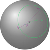 |
Fig. 1. Illustrative example of the IPN geometry for two detectors. One is in low-Earth orbit, and the other in an orbit around the forest moon of Endor. |
3. Methodology
Here we propose to estimate the inter-satellite time delay(s) of each GRB signal using a Bayesian (i.e., prior-regularized, likelihood-based) inference procedure built around a forward model designed to acknowledge the inherent stochasticity of the process by which the observational data are generated as shown in Fig. 2. To this end we suppose that the GRB emits a stream of photons distributed as the realization of a Poisson process indexed by time with a time-varying intensity such that each detector, di for i ∈ 1, …, Ndet, receives a portion of these photons along its unique line of sight. The effective temporal intensity function of each received signal, Si(t), is thus identical modulo its specific source-to-detector time delay, which for convenience we define with respect to the i = 1 labeled detector as Δti with Δt1 = 0, hence Si(t)≡S(t + Δti). We further suppose that each detector receives an independent background signal also distributed as a Poisson process with an intensity, Bi(t), combining additively with the GRB signal towards a Poisson process with total intensity function, Ci(t) = Si(t)+Bi(t).
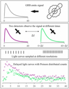 |
Fig. 2. Illustrative sketch of the problem as well as the framework for our forward model. A GRB emits a signal which is detected at two different times in detectors at different locations. These signals are translated into data sampled with different temporal resolutions and different detector effective areas resulting in two light curves which are delayed with respect to each other. |
Due to engineering constraints, different detectors can have different energy-dependent effective areas, thus breaking the above assumption that the observed signal will be exactly matched in structure between the detectors. This issue can be addressed within the hierarchical modeling framework by folding the signal model through each detector’s response function, either fitting for or assuming a spectral signal shape. For simplicity of exposition and to reduce the computational burden we assume here that neither detector suffers energy dispersion, but will allow for the effective area of each to vary by a scale factor, Ai, such that now Ci(t) = AiSi(t)+Bi(t). Also note that rather than fitting for a time difference directly, we can parameterize the time difference as a function of pgrb therefore allowing only time differences that would properly place the GRB’s location in the sky; that is,
therefore excluding time differences longer than  .
.
3.1. Likelihood
At the top level of our hierarchical model is the likelihood function, ℒ(⋅), for the observed process of photons arriving at our set of detectors, {ci(t)}i = 1, …, Ndet,

Here we use the notational form, ℒ(data|parameters), defining the likelihood as the probability density of the observed data conditional on a complete set of parameters characterising the assumed distribution of the sampling process. The second step is a factorization into product form since the realized Poisson process of photons arriving at each detector is conditionally independent once the mean intensity function, Ci(t), for each is specified. While the signal received in each is the realization of continuous time Poisson process (i.e., a randomly sized set of photons with unique arrival times), a discretization into counts per small equal unit of time is imposed by the detector read out. Hence, we write the likelihood in each as the product of ordinary Poisson distributions, 𝒫(mean expected count)[observed count], for the photon count over bins of width, δt, in the observing window from time, t0, to time, t0 + δt × Nbins, thus
![Mathematical equation: $$ \begin{aligned} \mathcal{L} \left(c_i(t)|C_i(t)\right) = \prod _{j=1,\dots ,N_\mathrm{bins} } \mathcal{P} \left(\int _{t_0+(j-1)\delta t}^{t_0+j\delta t} \mathrm{d}t^\prime C_i\left(t^{\prime }\right)\right)\left[ c_i(t)\right]. \end{aligned} $$](/articles/aa/full_html/2021/10/aa39461-20/aa39461-20-eq6.gif)
We note that for later computational convenience we treat the signal model here as if constant over the width of each temporal bin, taking the value at the mid-point of each bin as our reference.
3.2. GRB signal model
From the forward modeling perspective, the challenge now is to construct an appropriate probabilistic representation of the expected distribution of latent (noise-free) signal shapes, S(t), that may arise from observable GRB events. Without a guiding physical model for the evolution of GRB light curves and with respect to the sheer diversity of shapes on record over the thousands of GRBs detected to-date, we follow here a Bayesian non parametric approach (Hjort et al. 2010). That is, we adopt a rich stochastic process prior as the hypothetical distribution of possible latent signal shapes, supposing that the latent signal corresponding to any given GRB is a single realization from this process. A convenient and well-studied choice for this purpose is the Gaussian process (GP), which prescribes a multivariate Normal distribution over any index set of observed time points and is characterized by a mean function and a covariance function pair (Williams & Rasmussen 1996). Astronomical applications of Gaussian process-based modeling include the correction of instrumental systematics in stellar light curves to assist exoplanet detection (Aigrain et al. 2016), reverberation mapping of accretion disks around black holes with X-ray time series (Wilkins 2019) and modeling the variability in lensed quasars to estimate cosmological parameters (Suyu et al. 2017). As in the generalized linear model setting (where the exponential and logarithm are used as the transform and its inverse to map an unconstrained linear regression prediction on ℝ to the ℝ+ constrained support of the Poisson or negative binomial expectation; Hilbe et al. 2017), we apply an exponentiation to the Gaussian process within our hierarchical model, such that in fact it is the logarithm of the signal that is assumed to follow this distribution, that is, log S(⋅)∼GP3.
A straight-forward approach to Gaussian process modeling (as followed in the astronomical examples noted above) is to build a valid mean function and covariance function pair by choosing a constant for the former (i.e., μ(t) = c) and a stationary, kernel-based prescription for the latter,

Here the kernel function, K(⋅), may be composed of one or more (in summation) standard analytic forms known to correspond to valid covariance functions (in particular, to be non negative definite). For instance, the squared-exponential kernel, defined as
with σ an amplitude scale parameter and b an inverse length-scale (or “band-width”) parameter. The term “stationary” refers to the observation that such a kernel function takes only the time delay (or, more generally, distance) between points as its argument, such that the degree of covariance between points a fixed lag apart is imagined constant over the entire domain of the latent signal. Computing the likelihood of a realization of the latent signal at N distinct observation times requires construction and inversion of the full N × N covariance matrix, with a cost that naively scales in proportion to N3. Computational efficiency gains to scale of order Nlog2N can, however, be made with sophisticated inversion strategies for some of these commonly-used kernels (Ambikasaran et al. 2015).
In this analysis we follow an alternative approach to approximate a non stationary kernel using random Fourier features (RFFs; Rahimi & Recht 2008). The RFF approximation makes use of Bochner’s theorem (Bochner 1934) which describes a correspondence between each normalized, continuous, positive definite kernel on the real line and a probability measure in the spectral space of its Fourier transform. For example, the spectral measure, πK(ω), corresponding to a normalized version of the squared exponential kernel defined above is the zero-mean Normal distribution with standard deviation equal to the inverse length-scale, b, i.e., πK(ω) = 𝒩(0, b)[ω]. Once the corresponding spectral measure is identified for a given kernel, a RFF approximation may begin by drawing k (typically k < N) frequencies, ω(i) = 1, …, k ∼ πK(ω) to form a so-called “random feature matrix”, ϕ, with N rows (one per observed time point) of k sine and k cosine terms in the columns, i.e.,
![Mathematical equation: $$ \begin{aligned} \boldsymbol{\phi } =&\left[ \sin \left(2\pi \omega ^{(1)} \boldsymbol{t}\right), \ldots , \sin \left(2\pi \omega ^{(k)} \boldsymbol{t}\right),\right.\\& \left.\cos \left(2\pi \omega ^{(1)} \boldsymbol{t}\right), \ldots , \cos \left(2\pi \omega ^{(k)} \boldsymbol{t}\right)\right]. \end{aligned} $$](/articles/aa/full_html/2021/10/aa39461-20/aa39461-20-eq9.gif)
The RFF version of the GP prior on the latent signal may then be constructed as a regularized linear regression of features as
That is, β is formed as a length 2k column vector of elements with independent standard Normal distributions. For reference, the corresponding covariance matrix may be computed as  , which is similar to the strategy employed in some X-ray timeseries analyses (Zoghbi et al. 2012). An accessible introduction to the random Fourier feature approximation, albeit from the perspective of spatial Gaussian random fields rather than timeseries, is given by Milton et al. (2019).
To allow greater flexibility in our representation of the latent GRB signal we take an extension of the random Fourier features method to define a non stationary kernel. As described in Ton et al. (2018) (and see also Remes et al. 2017), Yaglom’s generalization of Bochner’s theorem (Yaglom 1987) can be used to show that spectral measures on product spaces of frequencies give rise to non stationary kernels. In this case the random Fourier feature approximation is made as ϕNS = ϕ1 + ϕ2 where the frequencies used in ϕ1 and ϕ2 are drawn from a joint distribution, πK(ω1, ω2). In this case we take an analog of the square exponential kernel with
![Mathematical equation: $$ \begin{aligned} \pi _K(\omega _1,\omega _2)=\mathcal{N} (0,b_1)[\omega _1]\times \mathcal{N} (0,b_2)[\omega _2]. \end{aligned} $$](/articles/aa/full_html/2021/10/aa39461-20/aa39461-20-eq12.gif)
Our GRB signal model is thus defined explicitly as
![Mathematical equation: $$ \begin{aligned}&\log S\left(t | b_1,b_2, \sigma _1, \sigma _2, \boldsymbol{\omega }_1,\boldsymbol{\omega }_2, \boldsymbol{\beta }_1, \boldsymbol{\beta }_2 \right)\nonumber \\&\qquad = \left[\sum _{i=1}^2 \frac{\sigma _i}{\sqrt{k}}\cos (b_i \boldsymbol{\omega }_i \otimes t) \right] \cdot \boldsymbol{\beta }_1 \nonumber \\ &\qquad \quad + \left[\sum _{i=1}^2 \frac{\sigma _i}{\sqrt{k}}\sin (b_i \boldsymbol{\omega }_i \otimes t) \right]\cdot \boldsymbol{\beta }_2. \end{aligned} $$](/articles/aa/full_html/2021/10/aa39461-20/aa39461-20-eq13.gif) (3)
(3)
3.3. Background signal model
To complete our forward model we need finally to specify a distribution for the expected background signals to be received by each detector. For simplicity we suppose here that each background is a constant function of Poisson counts with positive intensity, i.e., Bi(t) = Bi. Again, more complicated background signals can readily be handled within this hierarchical framework.
3.4. Directed acyclic graph view
In Fig. 3, we illustrate our hierarchical model as a directed acyclic graph. This diagrammatic mode of presentation highlights the connections between the parameters at each level of the hierarchical model and the data. Here, open circles represent latent variables to be inferred while closed circles indicate data. Quantities not enclosed in circles are constant information that do not exhibit measurement uncertainty. Finally, quantities enclosed in diamonds represent deterministic combinations of latent variables and/or fixed quantities.
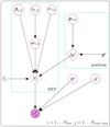 |
Fig. 3. Directed acyclic graph of our model. |
4. Validation
In order to demonstrate and validate our method, we have created a simulation package4 that allows for the virtual placement of GRB detectors throughout the solar system and creates energy-independent Poisson events sampled from a given light curve model. Using this package, we select a number of representative combinations of satellite configurations and light curve shapes and perform analyses on mock data simulated under each setting. We additionally compute the localization of the simulated GRB with the cIPN method to serve as a comparison. Our procedure for simulating mock datasets is described in Appendix A. In the following we first demonstrate the ability of the nazgul model to fit a single time series data set, and then proceed to fit two and three detector configurations to recover time delays and perform localizations. By repeating the simulation and localization process many times over, we confirm that the associated uncertainty intervals of the nazgul algorithm are well calibrated in a Frequentist (long-run) sense, i.e., that each quoted uncertainty interval contains the true source location with a frequency close to its nominal level.
4.1. Validation of pulse fitting with RFFs
Here we demonstrate the ability of RFFs to model simulated light curves with Poisson count noise. A GRB is simulated with four overlapping pulses each beginning five seconds after the pulse preceding it. In Fig. 4 we can see the posterior traces of the fit compared with the true light curve. We can check the reconstruction of the light curves via posterior predictive checks (Gabry et al. 2019, PPCs) where counts in each time bins are sampled from the inferred rate integrated over the posterior (see Fig. 5).
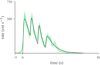 |
Fig. 4. Latent (black) and inferred (green traces) source light curve. |
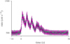 |
Fig. 5. Count rate data and PPCs from the single detector fit. The 1, 2 and 3σ regions are plotted in purple along with the data shown in green. |
We have checked that we are able to recover a variety of pulse shapes and combinations. Thus, even without the aid of a secondary signal from another detector, RFFs can learn the shape of the latent signal.
When the strength of the signal is decreased, we notice that the inferences become less constraining, but the overall ability of the model to reproduce the latent signal is sufficient to find properties of the light curve that can be time delayed.
We finally note that the light curve model used here is agnostic to the pulse shape as long as it is “fred-like”. Since we use the same light curve model for the cIPN as well as our new method, the conclusions on the relative strengths of these two triangulation methods are independent of whether or not our light curve model accurately reproduces measured GRB light curves and their range of parameters (e.g., number of peaks, spikiness or relative strength of consecutive peaks).
4.2. Two detector validation
The simulation for only two detectors allows us to validate the simplest configuration of detectors possible which results in a single annulus on the sky. For this simulation, the configuration consists of one detector in low-Earth orbit and another at an altitude mimicking an orbit in L1. The light curve shape chosen consists of two pulses and the detectors are given effective areas that differ by a factor of two. Each light curve is sampled at a different cadence (100 ms and 200 ms). Details are given in Tables 1 and 2.
Detector simulation parameters.
GRB simulation parameters.
We have found that choosing k = 25 features is sufficient for our purposes. Specific details of the fitting algorithm can be found in Appendix B. For the two detector fit, we compute credible region contours by computing the credible regions of Δt and translating these to annuli on the sky. We note that this is not the same as will be done for fits with more detectors.
As can be seen in Fig. 6, the algorithm correctly finds annuli enclosing the true position of the simulated GRB. The latent signal is recovered as shown in Fig. 6 and the PPCs adequately reproduce the data as seen in Fig. 7. We can examine the correlations between position and time that occur naturally due to our forward model approach in Fig. 8. By using different combinations of temporal binnings, we find that the result is not dependent on this parameter unless the binning is too large to resolve the time delay. Even in this case; however, we find that the result is only marginally affected with larger uncertainties on the time delay (Fig. 9).
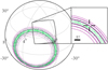 |
Fig. 6. Skymap of the two detector validation. The purple contours indicate the 1, 2, and 3σ credible regions with increasing lightness. The posterior samples are shown in green and the simulated position is indicated by the cross-hairs. |
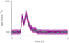 |
Fig. 7. Posterior predictive checks from fit in one of the detectors. The 1, 2 and 3σ regions are plotted in purple along with the data shown in green. |
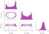 |
Fig. 8. Posterior density pair plots demonstrating the correlations between position an time delay. Simulated values are shown via gray lines. |
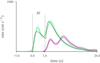 |
Fig. 9. Inferred posterior traces of the pulse models to in the two detectors (green and purple) compared with the non delayed simulated pulse model. |
We have repeated the experiment with same setup but different Poisson realizations of the light curves 500 times to ensure that our contours are statistically robust, i.e., that a give credible region is a proper representation of the probability that the latent value is recovered. Figure 10 shows the marginals of Δt for each fit to these simulations and clearly demonstrates that different Poisson realizations of the same light curve can lead to widely different Δt. Nevertheless, we can compute the number of times the simulated Δt falls within a given credible region with the expectation that the true value should fall M times within CRp such that p ≃ M/Nsims. We demonstrate that this condition is held in Fig. 11.
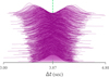 |
Fig. 10. Marginal distributions (purple) of fits to each two detector simulation ordered by their median’s distance to the true value (green). |
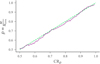 |
Fig. 11. Credible regions of Δt versus the fraction of times the true, simulated value is within that credible region. The green line represents a perfect, one-to-one relation. |
By simulating a grid of pulse intensities spanning three orders of magnitude, we can investigate the nazgul algorithm’s ability to reconstruct the time delay for a variety of pulse intensities. The same geometry and pulse shape is used except that the intensities of the pulses are modified to yield source significances ranging from ∼1σ to ∼200σ Here, we define significances with the likelihood ratio of Li & Ma (1983) and compute the significance over the peak flux duration of the pulse (see Appendix D). Fits are performed by binning each light curve to 100 ms. At low significance, the nazgul method is very uncertain about the true value of Δt, but at ∼5σ the method begins to have a trend at not only being accurate at recovering the true value but also becomes increasingly precise (see Fig. 12). Importantly, the nazgul method and resolve Δt appreciably below the resolution of the data for brighter simulated GRBs. These results are difficult to generalize as pulse shape and detector geometry can also play a role.
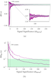 |
Fig. 12. Panel a: 1, 2, and 3σ uncertainties (purple) of Δt as a function of significance compared with the simulated value (green). Panel b: width of the 1 and 2σ uncertainties for the nazgul and cIPN (purple and green respectively) as a function of significance. The green region is below the resolution of the data and the dashed line appears at ∼5σ where the number of background-subtracted counts in the peak are displayed. |
4.3. Comparison with the classical method
The cIPN method of cross-correlating two background-subtracted light curves has had great success in localizing GRBs and other γ-ray transients (e.g., Cline et al. 1982; Hurley et al. 1998). However, part of the motivation of our work is to provide a newer algorithm with statistically robust uncertainties. Thus, we now run the classical algorithm on our simulated data sets and compare the results. It must be noted that this algorithm relies on two procedures which have known issues, namely, background subtraction and a Gaussian approximation to the Poisson distribution (for details see Pal’shin et al. 2013; Hurley et al. 2013, Appendix C).
First we examine the method on our example simulation. While our new algorithm is independent of binning and pre/post- source temporal selection, we find that the same is not true the cIPN cross-correlation approach, and different selections can have vastly different results. Thus, we choose a selection, having knowledge of the simulation parameters5 that encompasses the burst interval and has enough lag between the signals to fully map out the so-called reduced χ2-contour as a function of lag. We also chose different combinations temporal binnings for the light curves ranging from 50 to 200 ms; the coarser corresponding to what was used for the nazgul method. The results from two of the fits at different resolution is show in Fig. 13. We can see that the choice of binning immensely influences the confidence intervals. Additionally, the 1σ region misses the true value while the 3σ region is much larger than the nazgul posterior.
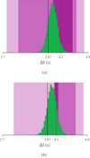 |
Fig. 13. Marginal distribution of Δt from the nazgul fit (green) compared with the 1, 2 and 3σ confidence intervals (purple) from the cIPN method for two different resolutions. The coarse resolution used for the nazgul fit (panel a) and a finer 50 ms resolution (panel b). The true value is shown as a black line and the mean value from the cIPN as a purple line. |
To see if these results can be generalized, we perform cross-correlation on each of the 500 simulations. We can repeat the exercise above and compute the fraction of fits that capture the simulated value given a confidence interval6. Figure 14 shows that for different temporal binnings, the credible intervals do not exhibit appropriate coverage. For coarser binnings, the coverage begins to approach expectations. This is likely due to the number of counts in each interval increasing for these binnings and thus satisfying the Gaussian approximation of the Poisson distribution. This poses severe difficulties for detector geometries which would need high-resolution to find sub-second time delays between light curves. We note that there are some combinations of resolution that result in adequate coverage in the 3σ intervals, but in situations involving real data, it would be impossible to know which combinations would be required.
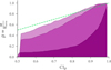 |
Fig. 14. Confidence intervals of Δt versus the fraction of times the true, simulated value is within that credible intervals. The green line represents a perfect, one-to-one relation. Here, coarser binnings are represented by lighter purple colors. |
Moreover, we can examine the relative widths of the uncertainties of the two methods at various confidence intervals. We find that while our algorithm is well behaved (see Fig. 15), the 1σ uncertainties of the cIPN method are smaller and (as shown above) underestimated, while the 3σ uncertainties are appreciably larger and likely over-estimated.
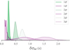 |
Fig. 15. Distributions of the relative widths of the uncertainties on Δt at three different credible levels from the classical (purple) and new (green) algorithm fits to simulations. |
We also examine how the cIPN method behaves with burst intensity. In Fig. 16 we compare the performance against the nazgul. All light curves were binned to 100 ms resolution. We again note, that in the actual use of the cIPN method, temporal resolution is chosen by hand to account for weak signals, but our procedure is chosen so that we can have direct comparisons. The 1σ behavior typically has a width of twice the resolution as expected, but even in the low-count regime (with some exceptions). The 2σ regions are better behaved similar to the nazgul method, but are much wider.
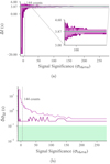 |
Fig. 16. Panel a: 1, 2, and 3σ uncertainties (purple) of Δt as a function of significance compared with the simulated value (green). Panel b: width of the 1 and 2σ uncertainties for the cIPN (purple) as a function of significance. The green region is below the resolution of the data and the dashed line appears at ∼5σ where the number of background-subtracted counts in the peak are displayed. |
Noting that the cIPN algorithm relies on a central limit theorem asymptotic of having many counts in a temporal interval, we simulate the same geometry but increase the flux by a factor of ten. We then repeat both methods on this brighter GRB. First, we fit with the nazgul algorithm with resolutions of 100 ms and 200 ms for each light curve respectively. We then use the cIPN method with a resolution of 50 ms. Figure 17 again compares the uncertainties of these two fits. In this case, the cIPN uncertainties behave properly, i.e., they are accurate, but surprisingly, the nazgul uncertainties are much more precise. Increasing the resolution to 50 ms for the nazgul has no effect and the precision of the result, but decreasing the resolution of the cIPN method to that used for the initial nazgul result increases the uncertainties by a fact of 2 as expected. However, it is possible to obtain sub-resolution uncertainties with the cIPN method by fitting a Gaussian to the reduced-χ2 curves as can be seen in Fig. 3 of Hurley et al. (1999).
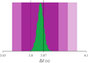 |
Fig. 17. Marginal distribution of Δt from the nazgul fit (green) compared with the 1, 2 and 3σ confidence intervals (purple) from the cIPN method for two different resolutions. The coarse resolution used for the nazgul fit. The true value is shown as a black line and the mean value from the cIPN as a purple line. |
We again examine the this behavior on multiple simulations. The nazgul maintains its adequate coverage, but the cIPN now begins to exhibit coverage that is semi-proper with fine temporal binnings. Though, the cIPN still underestimate 1σ intervals and overestimate 3σ intervals. The intervals for coarser binnings are too large in all cases. More importantly, the distribution of the widths for the cIPN method are appreciably larger than those of the nazgul. While we do not intend to do a comprehensive calibration of the cIPN method, we can demonstrate that there are issues with its ability to provide reliable uncertainties even in our toy setup. However, our newer method provides robust uncertainties with more precise 3σ contours. Also, it should be noted that the combinations of temporal resolutions and GRB intensities chosen do not always reflect the actual choices which are made by the IPN team. For example, if a weak GRB is being analyzed, coarser resolutions are chosen in an attempt to satisfy the number of counts required to satisfy the asymptotic conditions of the central limit theorem. Nevertheless, we find it important to demonstrate the frailty of these asymptotic methods as they are utilized in many places in the low-count regime of gamma-ray astrophysics (Figs. 18–20).
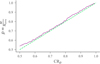 |
Fig. 18. Credible regions of Δt versus the fraction of times the true, simulated value is within that credible region. The green line represents a perfect, one-to-one relation. |
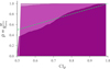 |
Fig. 19. Confidence intervals of Δt versus the fraction of times the true, simulated value is within that credible intervals. The green line represents a perfect, one-to-one relation. Here, coarser binnings are represented by lighter purple colors. |
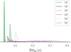 |
Fig. 20. Distributions of the relative widths of the uncertainties on Δt at three different credible levels from the classical (purple) and new (green) algorithm fits to simulations. |
4.4. Three detector validation
Extending upon our two detector validation, we now add a third detector to break the single-annulus degeneracy and further verify our algorithm. The above verification process is repeated with a new detector geometry as shown in Tables 3 and 4. This time, a single pulse is simulated again with all three detectors having different effective areas which are fitted for.
Detector simulation parameters.
GRB simulation parameters.
The nazgul algorithm clearly infers the correct position as shown in Fig. 21. However, the uncertainty regions do not mimic the diamond shaped uncertainties created by intersecting two annular uncertainty regions as is done by the cIPN (Sinha 2002). This is expected as we have demonstrated above that the two detector uncertainties regions are not correctly estimated and the way that these intersections are treated in the cIPN is reduced to a geometric rather than a statistical problem. The fact that our likelihood naturally includes all detector baselines in a single fit and treats the position of the GRB as a parameter rather than a downstream calculated quantity allows us to properly compute these uncertainty regions without reliance on asymptotic uncertainty propagation.
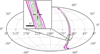 |
Fig. 21. Skymap of the three detector validation. The purple contours indicate the 1, 2, and 3σ credible regions with increasing lightness. The posterior samples are shown in green and the simulated position is indicated by the cross-hairs. |
We verify that the light curves of the simulated data are properly inferred via PPCs (see Fig. 22) and can examine the inferences of the latent pulse signal (see Fig. 23). We again can examine the natural correlation between position on the time delays in Fig. 24. Similar to the two detector geometry, the inference of the latent pulse shapes are not perfect owing to the Poisson realizations of the data. Nevertheless, the reconstruction is good enough to infer the time delays between the signals.
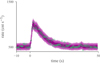 |
Fig. 22. Posterior predictive checks from fit in one of the detectors. The 1, 2 and 3σ regions are plotted in purple along with the data shown in green. |
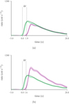 |
Fig. 23. Inferred posterior traces of the pulse models in the two detectors (green and purple) compared with the non delayed simulated pulse model for each of the detectors (topd1, 2 and bottomd1, 3). |
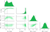 |
Fig. 24. Posterior density pair plots demonstrating the correlations between position an time delay. Simulated values are shown via gray lines. |
The inferred uncertainties on both time delays are also robust as we saw in the two detector case (see Fig. 25). However, we find that the same is again not true from the cIPN as shown in Fig. 26. Additionally, we find the same pattern of relative widths of the of the uncertainty regions for each of the baselines as was found in the two-detector case (see Fig. 27).
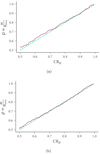 |
Fig. 25. Credible regions of Δt versus the fraction of times the true, simulated value is within that credible region for each detector baseline. The green line represents a perfect, one-to-one relation (topd1, 2 and bottomd1, 3). |
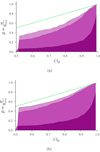 |
Fig. 26. Credible intervals of Δt versus the fraction of times the true, simulated value is within that credible intervals for each detector baseline. The green line represents a perfect, one-to-one relation. Here, coarser binnings are represented by lighter purple colors (topd1, 2 and bottomd1, 3). |
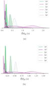 |
Fig. 27. Distributions of the relative widths of the uncertainties on Δt at three different credible levels from the classical (purple) and new (green) algorithm fits to simulations (topd1, 2 and bottomd1, 3). |
5. Discussion
We have presented a new approach to GRB localization via signal triangulation that demonstrates a forward modeling approach that is statistically principled. The approach does not require erroneous background subtraction, and is flexible enough to be improved upon with modifications that fully encompass the complications of real data. While the algorithm is much slower than the classical approach, IPN localizations are already much slower than other methods due to the latency of obtaining the data from multiple observatories, thus, we suspect little impact to the overall localization procedure. The computational time is; however, significant, typically requiring ∼30 min on a 40 core high-performance server. The runtime is influenced by the resolution of the light curves, but only mildly. Future improvements to the code will focus on decreasing this runtime. We have not addressed the issues of temporally varying backgrounds or spectrally evolving signals when they are detected by detectors with (1) different spectral windows and (2) high amounts of energy dispersion. We comment on each of these issues briefly below.
5.1. Temporally varying background
Detectors in low-Earth orbits such as Fermi/GBM operate in the presence of different background components that vary drastically during their orbits due to changing Earth/sky ratio, geomagnetic field and radiations belts. Thus, our simple assumption of a constant background would break down. Nevertheless, we can substitute this constant assumption with a temporal model such as a polynomial or even a secondary RFF. This will likely increase the uncertainty in the reconstructed localization, but will be statistically robust compared to background subtraction. This is independent of whether the background seen by different detectors is correlated or not, though in most cases it will not be correlated. We have made preliminary progress in this direction, but defer this work to a future study.
5.2. Spectrally evolving signals
For detectors with the same spectral window and energy-dependent effective area, the assumption that the time-varying signal observed in the data is the same is valid. However, if either of these two properties are not realized, then a more complex modeling is required. The simplest situation is when the detectors observe the same spectral window, but vary in their overall effective area. In this case, the latent signal can be multiplied by the known or modeled ratio of areas. In any other situation, a model for the spectrally evolving signal must be parameterized such that its shape can be fitted for and consequently, this shape must be folded through each detectors’ response. A similar approach is taken for the static case with the BALROG algorithm (Burgess et al. 2017; Berlato et al. 2019). While the approach is straight forward to implement, it will introduce computational expense to the algorithm. Moreover, the approach would require that the response functions of each instrument be publicly available and well calibrated. This extra spectral information would also enhance the ability to localize GRBs by adding an extra dimension to match across detectors. In the same way that BALROG uses the changing effective area of Fermi/GBM detectors to localize GRBs via their spectral shape, the same localization capability would work in tandem with the matching of time-differences in well separated detectors. Thus, we will pursue this issue in future work.
A current approximation to this issue could be to assume that at low-energies, where most of the signal is absorbed in the detector, the angle-dependent effective area evolves as a cosine from the optical axis of the detector. Thus, the change in amplitude of signal between various detectors is a function of the GRB position relative to the optical axis. To demonstrate this we have repeated the two detector validation but this time given each detector a cosine dependent effective area and adopted our algorithm appropriately. Thus, we set the amplitude of the signal arriving at the detector such the  where γ is the angle between the GRB and the optical axis of the detector. As can be seen in Fig. 28, the ring degeneracy of the triangulation method is broken and a more precise localization is achieved.
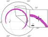 |
Fig. 28. Sky map of the two detector geometry when the detector is assumed to have an effective area that is proportional to the angle of the GRB w.r.t. its optical axis. Only the 1σ contour is shown for visual clarity. |
5.3. Refinements to statistical model and posterior approximation
Two theoretical issues with the proposed statistical model are worth noting, although they do not appear to limit the performance of the nazgul algorithm in any of the case studies examined in this simulation study. The first is that the credible intervals in Bayesian inference are not universally guaranteed to achieve Frequentist style coverages. That is, a 90% posterior credible interval is not guaranteed to offer at least a 90% coverage of the true parameter value in the long-run over mock datasets as would an “exact” Frequentist interval. The risks to the reliability of astronomical inference procedures due to supposing a priori that Bayesian intervals offer such coverage guarantees have been noted by Genovese et al. (2004), but remain little appreciated in the community. The model type studied here in which the target of interest is in effect a functional of a non parametric stochastic process prior is also similar to one in which pathological asymptotic results have been demonstrated in theoretical studies (Castillo 2012). For this reason we emphasize the importance of validation by simulated data in general, and in particular as further model complexity is added to increase the range of GRB observing scenarios covered by the nazgul algorithm.
The other theoretical issue of potential concern is with respect to behavior of Gaussian processes built on the squared exponential kernel. In particular, it is known that this kernel favors an aggressive smoothing which can lead to poor Frequentist style coverage of the latent function being approximated (Hadji & Szábo 2019). In this case we in fact use a non stationary version of the squared exponential kernel which allows for a non universal degree of smoothness, which might reduce exposure to this problem. On the other hand, it is evident that our chosen kernel and approximation via a small number of random Fourier features does lead to some degree of over-smoothing at the sharpest transition points, such as prior to initial burst up-tick in Fig. 4. Again, this does not seem to limit the accuracy of time delay recoveries, and there are possible advantages of a smooth kernel that might be working in our favor. For instance, a smoother kernel is less likely to attribute a cosmological origin to high background noise spikes, and can be better approximated with fewer random Fourier features than a less smooth kernel.
The current approach to posterior approximation is via MCMC simulation under a Hybrid Monte Carlo scheme (implemented in Stan). While this method offers a convergent approximation of the exact Bayesian posterior, it is in this case notably expensive in terms of computational resources and runtime. In similar problems it has been shown that first order approximations to the Bayesian posterior can be both adequate for uncertainty quantification and much more computationally efficient. For instance, in the setting of estimating time delays in gravitationally lensed quasar light curves, Tak et al. (2017) identified substantial computational gains from a profile-likelihood based approach. In our experiments with the nazgul algorithm we have been able to confirm an order of magnitude speed up in posterior sampling when the bandwidth parameter is held fixed, suggesting that a promising avenue of investigation may be to search for a heuristic bandwidth selection strategy to set this parameter to a reasonable value at the start of model fitting. An alternative may be to adapt the mesh-based approximation to Gaussian process inference offered by the INLA package (Lindgren et al. 2010), which can also accommodate non stationarity and offers speed ups equivalent to profile-likelihood based approaches. In either case it will be important to establish that any loss of accuracy in the uncertainty estimation stays within an acceptable tolerance to avoid losing the demonstrated coverage properties of the full posterior sampling scheme.
5.4. Methods for model misspecification
Finally, it is worth noting here that there are a number of methods, both established and emerging, for reducing the impact of model misspecification on parameter inference in either the Bayesian and Frequentist setting which may be worthwhile exploring in this context. Model misspecification occurs when the process from which the observed data are generated is not within the parametric family assumed by the modeler. In such cases the behavior of likelihood-based approaches is typically to converge towards the set of input parameters that minimize the Kullback–Liebler divergence with respect to the true sampling distribution. Depending on the nature of the misspecification this parameter set may be the same as, or close to, that which would be targeted if the assumed model were correct, but the behavior of the associated credible or confidence intervals associated with misspecified estimates tends to remain asymptotically incorrect. Methods such as Bayesian bagging (Huggins & Miller 2019), the weighted likelihood bootstrap (Spokoiny & Zhilova 2015), and the Bayesian bootstrap (Lyddon et al. 2019) can correct the tendency of these intervals to offer coverages lower than their nominal levels. While these three methods have been developed and studied almost exclusively under the iid (independent, identically distributed) data setting for simple parametric models, there is ongoing interest in extension to more complicated settings for which the GRB localization problem may prove a compelling case study.
6. Conclusion
The use of GRB IPN triangulations has been a successful enterprise, benefiting both the GRB and gravitational wave communities. However, we have shown that statistical uncertainties of the cIPN lack robustness. With our nazgul algorithm and the associated publicly available code7, we intend to work with the communities to increase the fidelity of the IPN with the aim of providing robust, statistically sound localizations in the on-going multi messenger era. We find that the method provides better accuracy and precision (see the smaller 2σ and 3σ contours in Figs. 15, 27). We foresee that issues will arise when dealing with real data, however, these issues exist for the cIPN as well. Given the success of the cIPN to locate many GRBs, we believe that these issues will be mitigated. It was brought to our attention (K. Hurley, priv. comm.), that attempts to obtain time delays via the fitting of functional forms to the data of the Vela satellites (Strong et al. 1974) though this work was never published.
There are also technical benefits to our approach due to the fact that Bayesian inference produces probabilities directly. First, our localization marginals can be directly convolved with other posteriors such as those of BAYESTAR (Singer & Price 2016), BALROG (Burgess et al. 2017), or any tool that also produces a localization posterior. Along these lines, we can also distribute the localizations in either HEALPix (Gorski et al. 2005) or the newer multi order coverage maps (MOC, Fernique et al. 2015) allowing rapid and direct access to the underlying location information without the need for pseudo localization combination techniques.
We further note that the methods developed here extend beyond GRB triangulation and can be used for other time-difference based studies which rely on signal variability with no a priori model such as the micro-lensing in quasars for the determination of dark matter content (Suyu et al. 2017) or for analysis of reverberation mapping of active galactic nuclei (Wilkins 2019). Even in cases of an existing a priori model, our methods might be advantageous if observing times are too short to beat the (timing) noise, such as X-ray millisecond pulsar navigation (Becker et al. 2018). Finally, these methods could be used in the search for gravitationally lensed GRBs (Grossman & Nowak 1994; Hurley et al. 2019) as they do not require the search for any a priori defined pulse shape or the use of cross-correlations.
This refers to the Tolkien characters in search of a magic ring, but in this case, annuli.
We note that this does not assume that the flux distribution is log-normal.
This is obviously not the case for real data and we expect our findings to not probe the systematics of source selection which may be considerable.
We note that there is a marked difference between a credible region and credible interval but for our purpose to calibrate coverage and with the Gaussian marginals we obtain, the difference is small.
Note that we fit for the changing effective area directly.
Acknowledgments
The authors are thankful for conversations with Kevin Hurley, Valentin Pal’shin, Alexander Nitz, Aaron Tohuvavohu and Thomas Siegert, in helping make the manuscript clearer. We thank the Max-Planck Computing and Data Facility for the use of the Cobra HPC system. Additionally, we thank Leo Singer for pointing us in the right direction to make sky maps. JMB acknowledges support from the Alexander von Humboldt Foundation. All software used in this publication including the framework and analysis scripts are publicly available. The work was made possible via Astropy (Astropy Collaboration 2018), matplotlib (Hunter 2007), numpy (Harris et al. 2020), SciPy (Virtanen et al. 2020), numba (Lam et al. 2015), Stan (Carpenter et al. 2017), arviz (Kumar et al. 2019), and ligo.skymap (Singer & Price 2016).
References
- Aartsen, M. G., Ackermann, M., Adams, J., et al. 2017, ApJ, 843, 112 [NASA ADS] [CrossRef] [Google Scholar]
- Aigrain, S., Parviainen, H., & Pope, B. 2016, MNRAS, 459, 2408 [NASA ADS] [Google Scholar]
- Ambikasaran, S., Foreman-Mackey, D., Greengard, L., Hogg, D. W., & O’Neil, M. 2015, IEEE Trans. Pattern Anal. Mach. Intell., 38, 252 [NASA ADS] [CrossRef] [Google Scholar]
- Andrae, R., Schulze-Hartung, T., & Melchior, P. 2010, ArXiv e-prints [arXiv:1012.3754] [Google Scholar]
- Aptekar, R. L., Frederiks, D. D., Golenetskii, S. V., et al. 1995, Space Sci. Rev., 71, 265 [NASA ADS] [CrossRef] [Google Scholar]
- Astropy Collaboration (Price-Whelan, A. M., et al.) 2018, AJ, 156, 123 [Google Scholar]
- Becker, W., Kramer, M., & Sesana, A. 2018, Space Sci. Rev., 214, 30 [CrossRef] [Google Scholar]
- Berlato, F., Greiner, J., & Burgess, J. M. 2019, ApJ, 873, 60 [NASA ADS] [CrossRef] [Google Scholar]
- Betancourt, M. 2017, ArXiv e-prints [arXiv:1701.02434] [Google Scholar]
- Betancourt, M., & Girolami, M. 2013, ArXiv e-prints [arXiv:1312.0906] [Google Scholar]
- Bochner, S. 1934, Ann. Math., 35, 111 [CrossRef] [Google Scholar]
- Burgess, J. M., Yu, H.-F., Greiner, J., & Mortlock, D. J. 2017, MNRAS, 476, 1427 [Google Scholar]
- Carpenter, B., Gelman, A., Hoffman, M. D., et al. 2017, J. Stat. Softw., 76, 1 [NASA ADS] [CrossRef] [Google Scholar]
- Castillo, I. 2012, Sankhya A, 74, 194 [CrossRef] [Google Scholar]
- Cline, T. L., Desai, U. D., Teegarden, B. J., et al. 1982, ApJ, 255, L45 [NASA ADS] [CrossRef] [Google Scholar]
- Connaughton, V., Briggs, M. S., Goldstein, A., et al. 2015, ApJS, 216, 32 [Google Scholar]
- Fernique, P., Allen, M. G., Boch, T., et al. 2015, A&A, 578, A114 [NASA ADS] [CrossRef] [EDP Sciences] [Google Scholar]
- Gabry, J., Simpson, D., Vehtari, A., Betancourt, M., & Gelman, A. 2019, J. R. Stat. Soc. Ser. A, 182, 389 [CrossRef] [Google Scholar]
- Genovese, C. R., Miller, C. J., Nichol, R. C., Arjunwadkar, M., & Wasserman, L. 2004, Stat. Sci., 19, 308 [Google Scholar]
- Gorski, K. M., Hivon, E., Banday, A. J., et al. 2005, ApJ, 622, 759 [Google Scholar]
- Grossman, S. A., & Nowak, M. A. 1994, ApJ, 435, 548 [NASA ADS] [CrossRef] [Google Scholar]
- Hadji, A., & Szábo, B. 2019, ArXiv e-prints [arXiv:1904.01383] [Google Scholar]
- Harris, C. R., Millman, K. J., Walt, S. J. V. D., et al. 2020, Nature, 585, 357 [CrossRef] [PubMed] [Google Scholar]
- Hilbe, J. M., De Souza, R. S., & Ishida, E. E. 2017, Bayesian Models for Astrophysical Data: Using R, JAGS, Python, and Stan (Cambridge University Press) [CrossRef] [Google Scholar]
- Hjort, N. L., Holmes, C., Müller, P., & Walker, S. G. 2010, Bayesian Nonparametrics (Cambridge University Press), 28 [CrossRef] [Google Scholar]
- Huggins, J. H., & Miller, J. W. 2019, ArXiv e-prints [arXiv:1912.07104] [Google Scholar]
- Hunter, J. D. 2007, Comput. Sci. Eng., 9, 90 [NASA ADS] [CrossRef] [Google Scholar]
- Hurley, K., Kouveliotou, C., Harmon, A., et al. 1998, Adv. Space Res., 22, 1125 [NASA ADS] [CrossRef] [Google Scholar]
- Hurley, K., Briggs, M. S., Kippen, R. M., et al. 1999, ApJS, 120, 399 [NASA ADS] [CrossRef] [Google Scholar]
- Hurley, K., Kouveliotou, C., Cline, T., et al. 2000, ApJ, 537, 953 [NASA ADS] [CrossRef] [Google Scholar]
- Hurley, K., Pal’shin, V. D., Aptekar, R. L., et al. 2013, ApJS, 207, 39 [Google Scholar]
- Hurley, K., Svinkin, D. S., Aptekar, R. L., et al. 2016, ApJ, 829, L12 [NASA ADS] [CrossRef] [Google Scholar]
- Hurley, K., Tsvetkova, A. E., Svinkin, D. S., et al. 2019, ApJ, 871, 121 [NASA ADS] [CrossRef] [Google Scholar]
- Kozlova, A. V., Israel, G. L., Svinkin, D. S., et al. 2016, MNRAS, 460, 2008 [NASA ADS] [CrossRef] [Google Scholar]
- Kumar, R., Carroll, C., Hartikainen, A., & Martin, O. A. 2019, J. Open Source Softw., 4, 1143 [Google Scholar]
- Lam, S. K., Pitrou, A., & Seibert, S. 2015, https://doi.org/10.1145/2833157.2833162 [Google Scholar]
- Li, T. P., & Ma, Y. Q. 1983, ApJ, 272, 317 [NASA ADS] [CrossRef] [Google Scholar]
- Lindgren, F., Lindström, J., & Rue, H. 2010, An Explicit Link Between Gaussian Fields and Gaussian Markov Random Fields: The SPDE Approach (Citeseer) [Google Scholar]
- Lyddon, S., Holmes, C., & Walker, S. 2019, Biometrika, 106, 465 [Google Scholar]
- Meegan, C., Lichti, G., Bhat, P. N., et al. 2009, ApJ, 702, 791 [NASA ADS] [CrossRef] [Google Scholar]
- Milton, P., Coupland, H., Giorgi, E., & Bhatt, S. 2019, Epidemics, 29, 100362 [Google Scholar]
- Norris, J. P., Nemiroff, R. J., Bonnell, J. T., et al. 1996, ApJ, 459, 393 [NASA ADS] [CrossRef] [Google Scholar]
- Pal’shin, V. D., Hurley, K., Svinkin, D. S., et al. 2013, ApJS, 207, 38 [Google Scholar]
- Rahimi, A., & Recht, B. 2008, in Neural Information Processing Systems, eds. J. C. Platt, D. Koller, Y. Singer, & S. T. Roweis (Curran Associates, Inc.), 1177 [Google Scholar]
- Remes, S., Heinonen, M., & Kaski, S. 2017, in Advances in Neural Information Processing Systems, 4642 [Google Scholar]
- Rubinstein, R. Y., & Kroese, D. P. 2016, Simulation and the Monte Carlo Method, 3rd edn. (Wiley Publishing) [Google Scholar]
- Singer, L. P., & Price, L. R. 2016, Phys. Rev. D, 93, 024013 [NASA ADS] [CrossRef] [Google Scholar]
- Sinha, S. 2002, JApA, 23, 129 [NASA ADS] [Google Scholar]
- Spokoiny, V., & Zhilova, M. 2015, Ann. Stat., 43, 2653 [Google Scholar]
- Strong, I. B., Klebesadel, R. W., & Olson, R. A. 1974, ApJ, 188, L1 [NASA ADS] [CrossRef] [Google Scholar]
- Suyu, S. H., Bonvin, V., Courbin, F., et al. 2017, MNRAS, 468, 2590 [Google Scholar]
- Tak, H., Mandel, K., Van Dyk, D. A., et al. 2017, Ann. Appl. Stat., 11, 1309 [Google Scholar]
- Ton, J.-F., Flaxman, S., Sejdinovic, D., & Bhatt, S. 2018, Spatial Stat., 28, 59 [Google Scholar]
- Vedrenne, G., Roques, J. P., Schönfelder, V., et al. 2003, A&A, 411, L63 [NASA ADS] [CrossRef] [EDP Sciences] [Google Scholar]
- Vianello, G. 2018, ApJS, 236, 17 [NASA ADS] [CrossRef] [Google Scholar]
- Virtanen, P., Gommers, R., Oliphant, T. E., et al. 2020, Nat. Methods, 17, 261 [Google Scholar]
- Wilkins, D. R. 2019, MNRAS, 489, 1957 [NASA ADS] [CrossRef] [Google Scholar]
- Wilks, S. S. 1938, Ann. Math. Stat., 9, 60 [Google Scholar]
- Williams, C. K., & Rasmussen, C. E. 1996, in Advances in Neural Information Processing Systems, 514 [Google Scholar]
- Yaglom, A. M. 1987, Basic Results, 1, 526 [Google Scholar]
- Zoghbi, A., Fabian, A., Reynolds, C., & Cackett, E. 2012, MNRAS, 422, 129 [NASA ADS] [CrossRef] [Google Scholar]
Appendix A: Simulations
To demonstrate the method, we designed a simulation package that allows us to create count light curves from any configuration of GRB sky position, and spacecraft orbit. To establish the geometry of the simulation a configuration file in YAML format is used. The user specifies the sky location of the GRB and its distance from the Earth. Then, for each GRB detector, the location is specified as the sky location and altitude above the Earth. The detector’s optical axis or pointing direction is specified as a sky coordinate along with the detector’s effective area in cm2. For simplicity, the effective area decreases as the cosine of the angle from the pointing direction’s normal vector. An example is given below:
# Specify the GRB parameters
grb:

        # Location and distance (degrees and Mpc)
        ra: 20.
        dec: 40.
        distance: 500.

        # lightcurve
        # if arrays are used then
        # multiple pulses are created
        K: [400.,400 ] # intensity
        t_rise: [.5, .5,] # rise time
        t_decay: [4, 3,] # decay time
        t_start: [0., 4.] # start time

# Specify the detectors
# each entry is treated as
# the name of the detector
detectors:

        det1:

            # 3D position is separated into
            # sky location (GCRS) and altitude
            ra: 40.
            dec: 5.
            altitude: 1500000. # km
            time: '2010-01-01T00:00:00'

            # optical axis of the detector

            pointing:
               ra: 20.
               dec: 40.

            effective_area: 1.

        det2:

          ra: 60.
          dec: 10.
          altitude: 500
          time: '2010-01-01T00:00:00'

          pointing:

               ra: 20.
               dec: 40.

            effective_area: .5
The remaining information is the shape of the light curve. The shape we use for the simulation is that of Norris et al. (1996) which specifies a simple pulse that rises and decays in time.
 (A.1)
(A.1)
Here, K is the amplitude of the pulse at the peak, τr is the rise time constant, and τd is the decay time constant. Any synthetic GRB within the framework can be composed of multiple Norris-like pulses.
Once the user specifies the parameters, the detectors are ordered by the arrival time of the GRB photons and a time-system is established between all the detectors such that the T0 or reference time is the arrival of the first photon at the detector closest to the GRB. Once this time system is established, individual photon events are sampled according to an inhomogeneous-Poisson distribution following the intrinsic pulse shape specified and weighted by each detectors’ effective area. The photons arrival times are sampled via an inverse cumulative distribution function (CDF) rejection sampling scheme (Rubinstein & Kroese 2016).
Assume we want to know how long one must wait (T) until a new photon arrives when our counts are Poisson distributed with constant rate λ.
 (A.2)
(A.2)
which tells us that the waiting times are exponentially distributed. Thus, we need to inverse CDF sample the exponential distribution to sample arrival times of photons. The CDF of the exponential distribution is
 (A.3)
(A.3)
thus we need to solve
 (A.4)
(A.4)
where u ∼ U(0, 1). This yields
 (A.5)
(A.5)
which is invariant to translations of u and thus we arrive at the equation to sample for the time between events.
 (A.6)
(A.6)
This allows us to sample a constant rate as is done for our background. We start sampling at the start time of the light curve, and continue until a specified tmax. As the rate for the signal evolves with time, we implement a further rejection sampling step that thins the arrival times according to the evolving λ(t) = s(t; K, τr, τd). This is done by first sampling a waiting time t and computing the λ(t). A draw from p ∼ U(0, 1) is made and the sample is accepted if p ≤ λ(t) as shown in Fig. A.1.
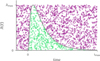 |
Fig. A.1. A demonstration of the rejection sampling from a Norris-like pulse shape where accepted samples are shown in green and rejected samples are shown in purple. |
Thus, the simulated events observed in each detector can be arbitrarily binned into any required cadence for the purpose of our analysis. Code and examples are available here.
Appendix B: Fitting algorithm
The high-dimensionality of this model requires a sampling algorithm capable of constructing the posterior accurately. For this, we choose the enhanced NUTS algorithm (Betancourt 2017) implementation in Stan (Carpenter et al. 2017). For every chain, we use 1000 warmup and 1000 sample iterations.
For the parameterization of the RFFs, we note that sampling for ω1, 2 provided more robust estimates than choosing them randomly. However, placing a prior of ω1, 2 ∼ 𝒩(0, b1, 2) creates a one-way normal (Betancourt & Girolami 2013) resulting in a funnel geometry. Thus, we choose a non centered parameterization such that  and
and  . We also found that a more efficient parameterization which resulted in no divergences required sampling the scale-length (l) or inverse of b normalized to the boundaries of the time series. This removed divergent transitions near the boundaries of the b marginal distributions. The algorithm proceeds as follows:
-
The integer count data, space craft position vectors in GCRS, and number of random features are loaded into Stan.
-
The GRB location prior is parameterized as a unit Cartesian 3-vector i.e., uniform on the sky.
-
 are given unit priors.
 -
l are sampled from weakly-informative priors bounded but the length of the time series and
 .
. -
β1,2 are give unit normal priors.
-
All scale parameters are given log normal priors.
-
A given detector is set as the reference detector from which all time-differences are computed. For each sample, the time delays are computed given the sampled GRB sky position.
-
S(t;b1,2,ω1,ω2,β1,β2) is computed for the reference detector and the time differences for all other detectors are used to compute the delayed signal.
-
The background level is estimated.
-
Each detectors’ signal and background are summed and compared to the observed counts via a Poisson likelihood.
In order to increase the speed of the algorithm, we have spilt the computation of the likelihood across several threads via Stan’s reduce_sum functionality. We have observed that the problem scales quasi-linearly with the number of threads. All fits checked for convergence, high effective sample size, and required to be divergence free. We note that sporadic divergences appear even after re-parameterization but can be removed by slightly decreasing the adaptive step-size. Code and examples are available here.
Appendix C: Cross-correlation algorithm for cIPN
We briefly describe our implementation of the cross-correlation algorithm to mimic the approach taken in the cIPN (for explicit details, see e.g., Pal’shin et al. 2013; Hurley et al. 2013). Assuming we have two light curves binned to resolution δ such that the total counts in each light curve time are c1, 2(ti) = c1, 2; i. With a known background one can subtract background counts from the total light curve. We denote these background subtracted counts as  . Now, a pseudo-statistic can be constructed such that
 (C.1)
(C.1)
where j indicates multiples of the base resolution. Here, s is the ratio of total counts in each light curve which is a heuristic way to account for the effective area varying across detectors8. Finally,  are the ubiquitously used estimators for the Poisson variance. Confidence intervals are then constructed via the relation
 (C.2)
(C.2)
Here, N − 1 indicates the number of degrees of freedom which are the number of time intervals. We can immediately identify points where this formalism can breakdown. At fine temporal resolutions, the estimator for the Poisson variance deviates from its central limit theorem approximation. Moreover, if there are zero counts in the intervals, the equation diverges. Secondly, the approximation of χ2 rarely holds and even more so for pseudo-statistics and the number of degrees of freedom is very dependent on the structure of the problem (Andrae et al. 2010). Lastly, it is well-known that the subtraction of two Poisson rates results in Skellam rather than Poisson distributed data. Depending on how background is subtracted, it may not even be the case that two Poisson rates are subtracted. For example, if the background is estimated via a model fit then the subtraction of the inferred counts must propagate the uncertainty of these inferences which will lead to a more complex form of statistic (Vianello 2018). The combination of approximations and asymptotics required for this approach understandably lead to uncertainties that do not provide adequate coverage.
Appendix D: Significance
It is well known (Li & Ma 1983; Vianello 2018) that using simple ratios of total and background counts rather than likelihood ratios leads to biased estimates of significance in counting experiments. This can also lead to overconfidence in when the asymptotics of the central limit theorem are reached. Therefore, in this work we employ the measure of significance derived in Li & Ma (1983) where we measure the counts in a temporally off-source region and compare it to the total counts at the peak of the pulse and adjust for the exposure differences. We can examine the significance as a function of background subtracted counts in Fig. D.1 where we have subtracted the total observed counts by the true background rate multiplied by the exposure.
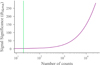 |
Fig. D.1. Significance as a function of background subtracted source counts. |
All Tables
All Figures
|
Fig. 1. Illustrative example of the IPN geometry for two detectors. One is in low-Earth orbit, and the other in an orbit around the forest moon of Endor. |
| In the text | |
|
Fig. 2. Illustrative sketch of the problem as well as the framework for our forward model. A GRB emits a signal which is detected at two different times in detectors at different locations. These signals are translated into data sampled with different temporal resolutions and different detector effective areas resulting in two light curves which are delayed with respect to each other. |
| In the text | |
|
Fig. 3. Directed acyclic graph of our model. |
| In the text | |
|
Fig. 4. Latent (black) and inferred (green traces) source light curve. |
| In the text | |
|
Fig. 5. Count rate data and PPCs from the single detector fit. The 1, 2 and 3σ regions are plotted in purple along with the data shown in green. |
| In the text | |
|
Fig. 6. Skymap of the two detector validation. The purple contours indicate the 1, 2, and 3σ credible regions with increasing lightness. The posterior samples are shown in green and the simulated position is indicated by the cross-hairs. |
| In the text | |
|
Fig. 7. Posterior predictive checks from fit in one of the detectors. The 1, 2 and 3σ regions are plotted in purple along with the data shown in green. |
| In the text | |
|
Fig. 8. Posterior density pair plots demonstrating the correlations between position an time delay. Simulated values are shown via gray lines. |
| In the text | |
|
Fig. 9. Inferred posterior traces of the pulse models to in the two detectors (green and purple) compared with the non delayed simulated pulse model. |
| In the text | |
|
Fig. 10. Marginal distributions (purple) of fits to each two detector simulation ordered by their median’s distance to the true value (green). |
| In the text | |
|
Fig. 11. Credible regions of Δt versus the fraction of times the true, simulated value is within that credible region. The green line represents a perfect, one-to-one relation. |
| In the text | |
|
Fig. 12. Panel a: 1, 2, and 3σ uncertainties (purple) of Δt as a function of significance compared with the simulated value (green). Panel b: width of the 1 and 2σ uncertainties for the nazgul and cIPN (purple and green respectively) as a function of significance. The green region is below the resolution of the data and the dashed line appears at ∼5σ where the number of background-subtracted counts in the peak are displayed. |
| In the text | |
|
Fig. 13. Marginal distribution of Δt from the nazgul fit (green) compared with the 1, 2 and 3σ confidence intervals (purple) from the cIPN method for two different resolutions. The coarse resolution used for the nazgul fit (panel a) and a finer 50 ms resolution (panel b). The true value is shown as a black line and the mean value from the cIPN as a purple line. |
| In the text | |
|
Fig. 14. Confidence intervals of Δt versus the fraction of times the true, simulated value is within that credible intervals. The green line represents a perfect, one-to-one relation. Here, coarser binnings are represented by lighter purple colors. |
| In the text | |
|
Fig. 15. Distributions of the relative widths of the uncertainties on Δt at three different credible levels from the classical (purple) and new (green) algorithm fits to simulations. |
| In the text | |
|
Fig. 16. Panel a: 1, 2, and 3σ uncertainties (purple) of Δt as a function of significance compared with the simulated value (green). Panel b: width of the 1 and 2σ uncertainties for the cIPN (purple) as a function of significance. The green region is below the resolution of the data and the dashed line appears at ∼5σ where the number of background-subtracted counts in the peak are displayed. |
| In the text | |
|
Fig. 17. Marginal distribution of Δt from the nazgul fit (green) compared with the 1, 2 and 3σ confidence intervals (purple) from the cIPN method for two different resolutions. The coarse resolution used for the nazgul fit. The true value is shown as a black line and the mean value from the cIPN as a purple line. |
| In the text | |
|
Fig. 18. Credible regions of Δt versus the fraction of times the true, simulated value is within that credible region. The green line represents a perfect, one-to-one relation. |
| In the text | |
|
Fig. 19. Confidence intervals of Δt versus the fraction of times the true, simulated value is within that credible intervals. The green line represents a perfect, one-to-one relation. Here, coarser binnings are represented by lighter purple colors. |
| In the text | |
|
Fig. 20. Distributions of the relative widths of the uncertainties on Δt at three different credible levels from the classical (purple) and new (green) algorithm fits to simulations. |
| In the text | |
|
Fig. 21. Skymap of the three detector validation. The purple contours indicate the 1, 2, and 3σ credible regions with increasing lightness. The posterior samples are shown in green and the simulated position is indicated by the cross-hairs. |
| In the text | |
|
Fig. 22. Posterior predictive checks from fit in one of the detectors. The 1, 2 and 3σ regions are plotted in purple along with the data shown in green. |
| In the text | |
|
Fig. 23. Inferred posterior traces of the pulse models in the two detectors (green and purple) compared with the non delayed simulated pulse model for each of the detectors (topd1, 2 and bottomd1, 3). |
| In the text | |
|
Fig. 24. Posterior density pair plots demonstrating the correlations between position an time delay. Simulated values are shown via gray lines. |
| In the text | |
|
Fig. 25. Credible regions of Δt versus the fraction of times the true, simulated value is within that credible region for each detector baseline. The green line represents a perfect, one-to-one relation (topd1, 2 and bottomd1, 3). |
| In the text | |
|
Fig. 26. Credible intervals of Δt versus the fraction of times the true, simulated value is within that credible intervals for each detector baseline. The green line represents a perfect, one-to-one relation. Here, coarser binnings are represented by lighter purple colors (topd1, 2 and bottomd1, 3). |
| In the text | |
|
Fig. 27. Distributions of the relative widths of the uncertainties on Δt at three different credible levels from the classical (purple) and new (green) algorithm fits to simulations (topd1, 2 and bottomd1, 3). |
| In the text | |
|
Fig. 28. Sky map of the two detector geometry when the detector is assumed to have an effective area that is proportional to the angle of the GRB w.r.t. its optical axis. Only the 1σ contour is shown for visual clarity. |
| In the text | |
|
Fig. A.1. A demonstration of the rejection sampling from a Norris-like pulse shape where accepted samples are shown in green and rejected samples are shown in purple. |
| In the text | |
|
Fig. D.1. Significance as a function of background subtracted source counts. |
| In the text | |
Current usage metrics show cumulative count of Article Views (full-text article views including HTML views, PDF and ePub downloads, according to the available data) and Abstracts Views on Vision4Press platform.
Data correspond to usage on the plateform after 2015. The current usage metrics is available 48-96 hours after online publication and is updated daily on week days.
Initial download of the metrics may take a while.