| Issue |
A&A
Volume 663, July 2022
|
|
|---|---|---|
| Article Number | A102 | |
| Number of page(s) | 11 | |
| Section | Extragalactic astronomy | |
| DOI | https://doi.org/10.1051/0004-6361/202243189 | |
| Published online | 14 July 2022 | |
Improving INTEGRAL/SPI data analysis of GRBs
1
Max-Planck-Institut für extraterrestrische Physik, Giessenbachstraße 1, 85748 Garching, Germany
e-mail: This email address is being protected from spambots. You need JavaScript enabled to view it.
2
Institut für Theoretische Physik und Astrophysik, Universität Würzburg, Emil-Fischer-Str. 31, 97074 Würzburg, Germany
Received:
25
January
2022
Accepted:
25
March
2022
Abstract
The spectrometer on the international gamma-ray astrophysics laboratory (INTEGRAL/SPI) is a coded mask instrument observing since 2002 in the keV to MeV energy range, which covers the peak of the νFν spectrum of most gamma-ray bursts (GRBs). Since its launch in 2008, the gamma-ray burst monitor (GBM) on board the Fermi satellite has been the primary instrument for analysing GRBs in the energy range between ≈10 keV and ≈10 MeV. Here, we show that the spectrometer on board INTEGRAL, named ‘SPI’, which covers a similar energy range, can give equivalently constraining results for some parameters if we use an advanced analysis method. Also, combining the data of both instruments reduces the allowed parameter space in spectral fits. The main advantage of SPI over GBM is the energy resolution of ≈0.2% at 1.3 MeV compared to ≈10% for GBM. Therefore, SPI is an ideal instrument for precisely measuring the curvature of the spectrum. This is important, as it has been shown in recent years that physical models rather than heuristic functions should be fit to GRB data to obtain better insights into their still unknown emission mechanism, and the curvature of the peak is unique to the different physical models. To fit physical models to SPI GRB data and get the maximal amount of information from the data, we developed new open-source analysis software, PySPI. We apply these new techniques to GRB 120711A in order to validate and showcase the capabilities of this software. We show that PySPI improves the analysis of SPI GRB data compared to the INTEGRAL off-line scientific analysis software (OSA). In addition, we demonstrate that the GBM and the SPI data for this particular GRB can be fitted well with a physical synchrotron model. This demonstrates that SPI can play an important role in GRB spectral model fitting.
Key words: methods: data analysis / gamma rays: general / gamma-ray burst: general
© B. Biltzinger et al. 2022
 Open Access article, published by EDP Sciences, under the terms of the Creative Commons Attribution License (https://creativecommons.org/licenses/by/4.0), which permits unrestricted use, distribution, and reproduction in any medium, provided the original work is properly cited.
Open Access funding provided by Max Planck Society.
1. Introduction
Gamma-ray bursts (GRBs) are short transient bursts of X- and γ-rays (Klebesadel et al. 1973) with a typical active time of between a few milliseconds and a few hundred seconds for the prompt phase. After the prompt emission, there is a long-lasting afterglow phase when the ejecta interact with the interstellar medium (Mészáros & Rees 1997; Vietri 1997). GRBs are classified into two groups depending on the duration of the prompt emission (Kouveliotou et al. 1993). Long GRBs (prompt phase ⪆2 s) have been associated with the collapse of massive stars (Galama et al. 1998; Hjorth et al. 2003; Woosley & Bloom 2006), whereas short GRBs are caused by mergers of compact objects, such as neutron stars (Eichler et al. 1989; Abbott et al. 2017). In both cases there is consensus that the progenitor events of GRBs produce jetted relativistic outflows, which consist of several shells with different velocities, resulting in internal shell collisions (Rees & Meszaros 1994; Mochkovitch et al. 1995).
The true physical mechanism(s) responsible for the prompt emission of GRBs is a heavily debated topic (for a review, see Kumar & Zhang 2015). Two of the possible emission mechanisms are synchrotron (e.g., Daigne & Mochkovitch 1998; Bošnjak et al. 2009; Burgess et al. 2020) and photospheric emission (e.g., Goodman 1986; Pe’er et al. 2005; Beloborodov 2010; Lazzati et al. 2013). In the past, GRB data were often fitted with empirical functions like the Band function (Band et al. 1993) in order to decipher the preferred physical model from the fit parameters. In recent years, it has been shown that this approach can be misleading and that it is preferable to fit physical models directly to the data (Burgess et al. 2014, 2020; Oganesyan et al. 2019). A prominent example of this is the so-called ‘line of death’ for synchrotron emission (Crider et al. 1997; Preece et al. 1998), which states that synchrotron radiation cannot be the universal emission mechanism if fits with a Band function give a low-energy power law slope larger than −2/3. Burgess et al. (2020) showed that this conclusion is flawed and that one can fit GRB spectra well with a physical synchrotron model even though the same spectra violate the line of death if fitted with a Band function. Another proposed proxy for physical emission processes in GRBs is the spectral curvature of empirical model fits to GRB data (Yu et al. 2015; Axelsson & Borgonovo 2015). This too has been shown to be an inaccurate indicator of the emission process (Burgess 2019). Therefore, the use of physical models remains the best tool for deciphering the emission processes occurring in the relativistic outflows of GRBs.
In addition to the model used, the data also play an important role. Earlier analyses showed that the shape of the spectrum around the peak is a decisive feature. Therefore, we make use of the spectrometer (SPI) on the international gamma-ray astrophysics laboratory (INTEGRAL; Winkler et al. 2003) which provides 100 times higher spectral resolution in the 0.1–1 MeV band compared to the frequently used gamma-ray burst monitor (GBM) on board the Fermi satellite.
The spectrometer SPI (Vedrenne et al. 2003) is one of the instruments on board the INTEGRAL satellite, which was launched in 2002. It is a coded mask instrument, with a fully coded field-of-view of 16 degrees, covering an energy range between 20 keV and 8 MeV. The unprecedented energy resolution allows the identification of fine spectral features, such as nuclear decay lines (Roques et al. 2003; Diehl et al. 2006) and curvature in continuous spectra (Jourdain & Roques 2020).
The standard analysis of SPI GRB data is done within the INTEGRAL Offline Scientific Analysis (OSA) software (Courvoisier et al. 2003), including SPI-specific routines (Diehl et al. 2003). A two-step method is applied, whereby first only the photo peak response is used to incorporate the mask pattern on the detectors, and then an energy redistribution correction response is applied. This method was used in several works that fitted empirical GRB models to the SPI data (Malaguti et al. 2003; Mereghetti et al. 2003a,b; von Kienlin et al. 2003a,b; Beckmann et al. 2004; Moran et al. 2005; Filliatre et al. 2005, 2006; McBreen et al. 2006; Grebenev & Chelovekov 2007; McGlynn et al. 2008, 2009; Foley et al. 2008; Martin-Carrillo et al. 2014). The noteworthy exception of Bošnjak et al. (2014) is discussed separately below in Sect. 2.5. Apart from data handling, all previous analysis of GRB data from INTEGRAL/SPI used heuristic functions like the Band function, but not a physical model.
Here, we developed the pure Python-based analysis tool PySPI in order to provide an easy-to-use data-reduction and fitting tool while getting the maximal amount of information out of the data to progress to fitting physical models. This improves the analysis method in general, because we use the full response to forward model the expected spectra to the native SPI data space and use the correct likelihood to take the Poisson nature of the measurements into account. It also offers an interface that is easy to install and use. This work is structured as follows: In Sect. 2, we summarise the different methods and concepts for SPI GRB data analysis, and provide a detailed description of the new analysis method within PySPI in Sect. 2.4. Section 3 introduces the physical synchrotron model we used in the fits and Sect. 4 explains how we check whethre or not a fit is a good description of the data. We analyse the SPI and GBM data for GRB 120711A in Sect. 5 and conclude our results in Sect. 6.
2. SPI GRB analysis methods
All instruments, especially gamma-ray instruments, suffer from energy dispersion and finite energy resolution. The information about this is encoded in the response matrix, which gives the probability that a photon with a certain energy and starting position on the sky will be detected in one of the electronic channels of the detector. These response matrices are usually not invertible, and therefore we have to forward fold the photon spectrum through the response matrix into the data space of the detected counts and compare them using the correct likelihood. This is a general statement that also applies to SPI. In the following subsection, we first cover some general concepts for SPI and then the standard analysis method within OSA, as well as the method within our new analysis tool PySPI. The main difference is that the method in PySPI is a full forward-folding method, fulfilling the statement above, which results in maximising the information we can get from the data in the analysis.
2.1. Response
The response connects the photon spectrum to an expected detected count spectrum for a given source position. The response encapsulates all the information about the probability of a photon with a certain energy and origin to be detected in a certain electronic channel of the detector. This includes, for example, information about partial energy deposition of the photon in a crystal and the process that transforms the deposited energy into the electronic signal that is measured. The response is split into two components, namely the image response functions (IRFs) and redistribution matrix files (RMFs). The IRFs contain information about the total effective area over which a photon can interact with the detector and the RMFs contain information about the probability in which electronic channel the photon will be measured. For SPI, both these components were derived with extensive geometry and tracking (Geant) simulations (Sturner et al. 2003). The SPI IRF files give the total effective area for three different interaction types: (1) photo peak events; (2) non-photo-peak events that first interact in the Ge crystal, and (3) non-photo-peak events that first interact in passive material. These effective areas were calculated for 51 photon energies and on a 0.°5 grid out to 23.°5 from the on-axis direction. For each of the three interaction types, there is one RMF to define the shape of the redistributed spectra, assuming that this shape does not depend on the detector or the incident angles of the photons. The procedure used to construct the response includes several simplifications to keep the computational costs and storage space at manageable levels (Sturner et al. 2003). Re-simulating the response without these simplifications could improve the scientific output of SPI, but would be computationally very expensive, even today.
2.2. Electronic noise
According to Roques & Jourdain (2019), there are spurious events in the SPI data, which are photons with small energy (<100 keV) that get detected at a higher energy due to saturation of the analog front-end electronics (AFEE) by previous high-energy deposition. It is also known that these spurious events do not show up in events that also have a detection in the pulse shape discriminator (PSD) electronics. The reason for this is that the PSD electronics have a low-energy threshold of ≈450 keV and a high-energy threshold of ≈2700 keV (the exact values have been changed a few times during the mission; Roques & Jourdain 2019). Therefore, only events that deposit more than this low-energy threshold in the germanium crystal can trigger this electronic chain, which eliminates the < 100 keV events that are detected at the wrong energies by the AFEE. In Fig. 1, the feature at 1.5 MeV is nicely visible in the non-PSD events but is missing in the PSD events. Even though this problem is most significant in the area around 1.5 MeV, it is also important at lower energies > 400 keV. The electronic noise is not stable and depends on the signal strength (Roques & Jourdain 2019), and therefore it cannot be included in the response and has to be treated differently.
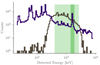 |
Fig. 1. Count spectrum for detector 0 integrated over 1000 s in revolution 1189. The non-PSD event count spectrum is drawn in purple and the PSD events in grey. The light green shaded area marks the energy range within the PSD energy thresholds (Roques & Jourdain 2019). The feature is clearly seen in the non-PSD events at 1.5 MeV (stronger green shaded area) and is not visible in the PSD events. |
2.3. INTEGRAL OSA software
As we are introducing new analysis software in this work, we want to compare it to the existing analysis software to check whether or not the results are in agreement. We briefly summarise the standard analysis tools for GRB analysis, which are part of the OSA software (Courvoisier et al. 2003).
Analysing GRB data from SPI with the OSA tools is a multi-step process. The first steps involve selecting the science window containing the GRB, the time intervals for active time and background time, and the energy bins for the analysis. One can either find the location of the GRB with SPIROS, which is an iterative source-removal algorithm for SPI data (Skinner & Connell 2003), or set it manually if it is already known. The next steps encompass the spectral fitting, which is done in another two-step procedure.
The first step in the spectral fitting with OSA is to use only the photo-peak response of the detectors. These responses depend on the source position, as this defines for example the absorption by the mask. With these responses and the measured data in the individual SPI detectors, taking into account the different background rates, a photon flux is fitted individually per energy channel. These pseudo photon fluxes are not the final result, as at this point, energy dispersion and detector energy resolution have not yet been accounted for. The pseudo photon flux data points are fitted with a spectral photon flux model and a correction response. The correction response, that is available through OSA, depends on the energy bins that are used and should account for energy dispersion. In this step, the energy channels are fitted simultaneously, as it is impossible to incorporate energy dispersion in a way that fits every energy channel individually. This fitting can be done in different spectral fitting software, such as XSPEC (Arnaud 1996) or the multi-mission maximum likelihood framework (3ML; Vianello et al. 2015).
2.4. PySPI
To fit SPI GRB data, we developed a new Python package PySPI (Biltzinger et al. 2022). Below, we summarise the main points of GRB analysis within PySPI.
2.4.1. Background
GRBs are transient sources with a typical duration of up to a few tens of seconds. Therefore, we can use the time intervals during a single pointed observation (science window) – when the transient source is not active – as an independent temporal off-source observation (see Fig. 2). This approach is similar to what is done with other instruments that use off-source observations to make independent background measurements. The probability distribution for the background model rates per energy channel is the Poisson distribution:
 (1)
(1)
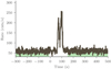 |
Fig. 2. Light curve for SPI detector 0 for GRB 120711A. The transient source is clearly visible as well as the constant background for the time when the transient is not active. The time interval we use for the independent background observation is marked with the green shaded area. |
where bi are the background rates per energy channel, Bi are the detected counts in the off-source observation, and tb is the exposure of the off-source observation.
2.4.2. Likelihood
With the defined background distribution, we can construct a likelihood, given by Eq. (2), that connects the source and background model with the Poisson process data of the background and active time interval via the response. Here, θ summarises all the parameters of the source model, Di are the measured counts in the selected active time interval of the transient source, mi(θ) are the predicted count rates from the model evaluated at the parameters θ, and td is the exposure of the selected active time interval:
 (2)
(2)
If there was a spectral model for the background, we would fit the background and the source model at the same time with the likelihood given in Eq. (2), but we do not have such a model for the SPI background. The background in SPI is dominated by the interaction of cosmic rays in the satellite material, which produces nuclear de-excitation line emission for example (Siegert et al. 2019). For this reason, the background consists of several hundred different nuclear lines (Siegert et al. 2019), which makes an accurate spectral model for the background impossible at present. However, we can marginalise over the parameters bi using only the simple fact that they cannot be negative, which leaves us with Eq. (3):
 (3)
(3)
The marginalisation is equivalent to integrating out the background rate parameter assuming a uniform prior from zero to ∞. Because solving this integral is computationally expensive, we use a profile likelihood as an auxiliary but still statistically sound figure of merit. For the profile likelihood, we use the fact that the derivative of the likelihood at its maximum is zero ( ). This defines the background rates bi, max (see Eq. (4)) that maximise the likelihood for a given model mi(θ) and observed quantities:
 (4)
(4)
These values are then substituted into the likelihood Eq. (2) to eliminate the bi dependency. This gives the exact solution for the maximum of the likelihood; for likelihood values close to the maximum, the assumption is that most of the likelihood in the integrand in Eq. (3) is in a small area around bi, max. This profile likelihood method has been used in many spectral analysis works (e.g., Loredo & Wasserman 1995; Burgess et al. 2019) and is also available in XSPEC (Arnaud 1996) as cstat and pgstat.
2.4.3. Response
In PySPI, we use the official response files, as described in Sect. 2.1, interpolate them to the wanted energy bins and source positions, and construct one response matrix incorporating all the information about the effective area and energy redistribution. During this process, we take into account that the mask is not absorbing 100% of the photons flying through it.
2.4.4. Electronic noise
In PySPI, one can select the energy range in which only the PSD events should be used to avoid including spurious events (see Sect. 2.2). To account for the larger dead time of the PSD electronics, an effective area correction can be either fixed to 85% (Roques & Jourdain 2019), or treated as a free parameter of the model.
2.4.5. General procedure
Every Ge detector is treated as an independent detector unit. The workflow during a fit step is a forward folding method: (1) sample model parameters, (2) calculate the model flux and responses individually for all detectors for the given source position, (3) fold the model with responses to get the predicted model counts in all detectors, (4) calculate the log-likelihood for all detectors, and (5) sum these log-likelihoods to get the total log-likelihood of the SPI data for the given model parameters. The BALROG (BAyesian Lo-cation Reconstruction Of GRBs) algorithm for localising GRBs with Fermi/GBM employs the same method (Burgess et al. 2018), which shows that forward folding allows one to localise photon sources with a non-imaging instrument. It is important to realise that the instruments SPI and GBM are fundamentally very similar; they both consist of individual detectors that have different responses for a given source position. In GBM, this is due to the different pointing directions of the detectors, and in SPI it is due to the varying obscuration by the mask. Even though SPI is defined as a coded-mask instrument, it does not require special treatment. The information that the mask encodes into the data is automatically included by using the different responses for the detectors and a forward folding method. A similar approach was used by DeLaunay & Tohuvavohu (2021) that introduces a new forward folding method to detect and localise faint GRBs with the coded mask instrument Swift/BAT.
2.4.6. Software interface
PySPI constructs a plug-in for 3ML (Vianello et al. 2015). This allows one to fit SPI data together with data from other instruments, such as Fermi/GBM1. PySPI is open source software, and is publicly available on GitHub (Biltzinger et al. 2022), including documentation with examples2.
2.5. Comparison of our method to Bošnjak et al. (2014)
Bošnjak et al. (2014) performed a joint analysis of SPI and IBIS (Imager on Board the INTEGRAL Satellite) data of GRBs and created a spectral catalogue of INTEGRAL GRBs (Ubertini et al. 2003). Bošnjak et al. (2014) construct a response for every SPI detector and forward fold the photon model directly into the data space of every detector, which is similar to our approach in this work. Following their paper, we see two main differences compared to our method, namely response generation and treatment of the electronic noise, and one ill-defined issue (background treatment).
For the response generation, Bošnjak et al. (2014) state that they calculate a response function taking into account the exposed fraction of each detector for the GRB position and that the net spectrum is zero for a completely shadowed detector. Therefore, we conclude that they used an idealistic mask with zero transparency at all energies. We on the other hand used the official response simulations that also include some transparency, especially at high energies. The second point is that the electronic noise is ignored completely in Bošnjak et al. (2014). Roques & Jourdain (2019) showed that the effect of the PSD events gets stronger for bright sources, and therefore it is important to account for this effect in the case of GRBs.
Concerning the background treatment, Bošnjak et al. (2014) argue that background subtraction is better than using a model template for the background within OSA, and cite Cash (1979) for their likelihood. Therefore, one would conclude that they used a Poisson likelihood on the background-subtracted data, but they also state that they provide on-burst and background spectra separately to XSPEC, which implies that no background subtraction was done before the fit. This was clarified with Ž. Bošnjak in a private communication during the refereeing process: in XSPEC, background and burst(-source) spectra were used separately, and no background subtraction was done for the fits.
Unfortunately, the software used to generate the data files and response files in Bošnjak et al. (2014) is not public and only the results for combined fits of SPI and IBIS data are shown. Therefore, we cannot directly compare our method and results with theirs. Also, Bošnjak et al. (2014) only used data up to 1 MeV for SPI, whereas with PySPI we can use the data up to higher energies (up to 8 MeV), which is needed to constrain the peak energy for GRB 1200711A, which is at ≈1.4 MeV (see Sect. 5.2).
3. Physical synchrotron model
We use pynchrotron3 to calculate the spectrum from a physical spectral synchrotron model. This model was previously used to successfully fit many single-pulse GRBs observed with Fermi/GBM in Burgess et al. (2020), which also includes a detailed description of the model. Here, we summarise the main points.
The core of the model is the assumption of some generic acceleration mechanism that constantly accelerates electrons into a power-law spectrum N(γ)∝γ−p between γinj and γmax. These electrons are cooled via the emission of synchrotron photons in a magnetic field. The resulting photon spectrum is the sum of the photon spectra at every time-step in the cooling process and is defined by five quantities: (1) the magnetic field strength (B), (2) the slope of the injected electron spectrum (p), (3) the lower boundary of the injected electron spectrum (γinj), (4) the upper boundary of the injected electron spectrum (γmax), and (5) the characteristic Lorentz factor the electrons cool to (γcool). There exists a strong degeneracy between B and γinj, as their combination sets the peak of the photon spectrum. Therefore, we fix γinj = 105 and only fit for B.
4. Model checking
How to decipher whether or not the fit of a model is a good description of the measured data is a very complicated and highly debated topic in the statistics community. Measurements like reduced χ2 rely on many assumptions; for example, that all the probability distributions in the problem are described as normal distributions (Andrae et al. 2010). This is not the case here, as the measurement process is a Poisson process. We therefore decided to use posterior predictive checks (PPCs) and quantile-quantile (QQ) plots.
For the PPCs, one simulates new data from the full posterior of the fit and the measurement process (see Eq. (5)) and compares them to the observed data (Gelman 2003). QQ plots use the same simulation process, but instead of comparing the observed data of every energy channel individually to the simulated data, one compares the cumulative counts of the observation and the simulations over energy channels (Wilk & Gnanadesikan 1968). QQ plots are very sensitive to weak systematic deviations of the model from the data.
 (5)
(5)
Here yobs are the observed data, P(θ|yobs) is the posterior distribution of the model parameters θ given the observed data, P(ysim|θ) is the probability of new data given the parameters of the model, and ysim are the simulated data.
5. Analysis
As an example, we analyse GRB 120711A, a bright, multi-pulse GRB with a precursor and a long emission period of ≈100 s. GRB 120711A was detected by SPI and GBM (Goetz et al. 2012; Gruber & Pelassa 2012). We look at one time interval with a duration of 10 s around the first bright peak in the light curve (see Fig. 3). From the detection of the afterglow with the X-ray telescope (XRT) onboard the Swift satellite, we have an accurate position of the GRB (RA = 94.°68, Dec = −71.°00 in J2000) (Beardmore & Evans 2012). The SPI data for GRB 120711A were previously analysed by Martin-Carrillo et al. (2014), but these authors only fitted the time-averaged spectrum over the T90 emission (between 0 and 115 s after the trigger) with an empirical exponential cutoff power-law model, while focusing on the post-GRB emission properties.
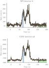 |
Fig. 3. Light curve for GRB 120711A in one GBM and one SPI detector. The green shaded area marks part of the time intervals used for the independent background observation and the blue shaded area is the active time interval used in the fit. |
First, we present our fit of the data with the empirical Band function, and show a comparison between the fit results using PySPI versus OSA (Sect. 5.1). We then check whether or not the results for SPI and GBM are in agreement (Sect. 5.2). Subsequently, we present our fit of the SPI and GBM data simultaneously with a physical synchrotron model, which was done to check whether or not including SPI in the analysis can reduce the allowed parameter space (Sect. 5.3).
For all GBM and PySPI fits, we added effective area correction parameters, allowing the total effective area of the individual detectors to vary with respect to each other in order to account for slightly different calibrations. To do this, we fixed the response of one of the detectors and fitted one parameter for every other detector. We constrain the effective area correction parameters to be between 0.7 and 1.3. All the fits use 3ML (Vianello et al. 2015) and the Bayesian sampling algorithm MultiNest (Feroz et al. 2009) to create posterior distributions of the parameters.
5.1. Comparing PySPI and OSA
We fit the SPI data of an identical time interval with a Band function within PySPI and OSA. Figure 4 shows the resulting posterior distributions of the fits. The results for the spectral shape from the two analysis techniques agree within their uncertainty regions, but PySPI can constrain the model more precisely (see Fig. 5).
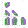 |
Fig. 4. Corner plot showing the Band function fit to the SPI data with PySPI and OSA with the data for GRB120711A. The results are in agreement, but PySPI constrains the parameters more precisely. |
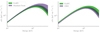 |
Fig. 5. Model posterior plots (95% confidence region) for the results with the Band function model and the data for GRB120711A. Left panel: results for the PySPI fit compared to the fit using OSA and right panel: PySPI fit compared to the GBM fit. |
5.2. Comparing SPI and GBM
We then analysed SPI data with PySPI and the GBM data with the GRB analysis within 3ML, again with a Band function. Figure 6 shows the results for these fits; we can see that the results for the spectral shape from SPI and GBM are in agreement. It also shows that the effective area calibrations for SPI and GBM are well aligned, with a difference of only ≈10% (K parameter), which is well within the uncertainties as specified in the corresponding instrument publications.
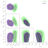 |
Fig. 6. Corner plot for the SPI fit with PySPI and the GBM fit to the data of GRB120711A. In this fit, we used a Band function as a spectral model. The spectral shapes for the SPI and GBM fits coincide within their uncertainty regions and the normalisation is off by ≈10%. |
5.3. Joint fit of SPI and GBM
We performed a joint fit of SPI and GBM data with a physical synchrotron model (see Sect. 3). Figure 7 shows the corner plots, Fig. 8 the spectra of the fitted models and Fig. 9 the data compared to the best-fit predicted counts for the individual and combined fits. The posterior distribution of the parameters from the GBM and the SPI fit agree within their uncertainty regions and the combined fit reduces the allowed parameter space. The physical synchrotron model was able to fit the data of GBM and SPI well, which is shown with PPC and QQ plots in Appendix B.
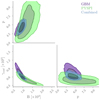 |
Fig. 7. Corner plot for the SPI fit with PySPI and the GBM fit to the data of GRB120711A. In this fit we used a physical synchrotron model (see Sect. 3) as a spectral model. The results from SPI and GBM agree within their uncertainty region and the combined fit provides better constraints on the parameter than the individual ones. |
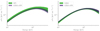 |
Fig. 8. Model posterior plots (95% confidence region) for the results with the physical synchrotron model and the data for GRB120711A. Left panel: results for the SPI fit compared to the combined fit and right panel: GBM fit compared to the combined fit. The combined fit reduces the allowed model space. |
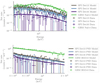 |
Fig. 9. Data (for GRB120711A) and best-fit model in count space for three of the SPI detectors and one of the NaI (BGO) detectors of GBM (upper and lower plot, respectively). The spectral model for this fit was a physical synchrotron model. |
6. Conclusion
We present a new analysis method for GRBs detected by INTEGRAL/SPI and the corresponding software package that uses this method. The PySPI software uses a proper forward-folding technique for each detector (see Sect. 2.4). To show that this improves the analysis of GRBs detected by SPI, we analysed GRB 120711A using the data from INTEGRAL/SPI and Fermi/GBM. The results for SPI with PySPI are in agreement with those from the INTEGRAL OSA software, but provide better constraints. Also, the resulting spectral shape for the fits with GBM and SPI data are in agreement and the relative calibration difference between SPI and GBM – which we conclude from the fits – is ≈10% or less. We show that the GBM as well as the SPI data for GRB 120711A can be fitted well with a physical synchrotron model and that combining the data in a simultaneous fit improves the parameter constraints. Consequently, SPI can play an important role in physical GRB model checking. The next steps will entail an analysis of all GRBs detected by SPI with different physical models and PySPI to check whether or not some of these models can be rejected with the SPI data. This will be covered in a future paper.
Acknowledgments
We thank Ž. Bošnjak for quickly responding to our inquery about the details of data handling in Bošnjak et al. (2014). B.B. acknowledges support from the German Aerospace Center (Deutsches Zentrum für Luft- und Raumfahrt, DLR) under FKZ 50 0R 1913. T.S. acknowledges support by the Bundesministerium für Wirtschaft und Energie via the Deutsches Zentrum für Luft- und Raumfahrt (DLR) under contract number 50 OX 2201. This work made use of the following software packages: 3ML (Vianello et al. 2015), Astromodels (Vianello et al. 2021), Matplotlib (Caswell et al. 2021), ChainConsumer (Hinton 2016; Hinton et al. 2020), OSA (Courvoisier et al. 2003), Numpy (Harris et al. 2020), MultiNest (Feroz et al. 2009, 2019; Feroz & Hobson 2008).
References
- Abbott, B. P., Abbott, R., Abbott, T. D., et al. 2017, ApJ, 848, L13 [CrossRef] [Google Scholar]
- Andrae, R., Schulze-Hartung, T., & Melchior, P. 2010, ArXiv e-prints [arXiv:1012.3754] [Google Scholar]
- Arnaud, K. A. 1996, in Astronomical Data Analysis Software and Systems V, eds. G. H. Jacoby, & J. Barnes, ASP Conf. Ser., 101, 17 [NASA ADS] [Google Scholar]
- Axelsson, M., & Borgonovo, L. 2015, MNRAS, 447, 3150 [NASA ADS] [CrossRef] [Google Scholar]
- Band, D., Matteson, J., Ford, L., et al. 1993, ApJ, 413, 281 [Google Scholar]
- Beardmore, A., & Evans, P. 2012, GCN Circular, 13442 [Google Scholar]
- Beckmann, V., Borkowski, J., Courvoisier, T. L., et al. 2004, Nucl. Phys. B, Proc. Suppl., 132, 301 [NASA ADS] [CrossRef] [Google Scholar]
- Beloborodov, A. M. 2010, MNRAS, 407, 1033 [NASA ADS] [CrossRef] [Google Scholar]
- Biltzinger, B., Burgess, J. M., & Siegert, T. 2022, J. Open Source Software, 7, 4017 [NASA ADS] [CrossRef] [Google Scholar]
- Bošnjak, C., Daigne, F., & Dubus, G. 2009, A&A, 498, 677 [NASA ADS] [CrossRef] [EDP Sciences] [Google Scholar]
- Bošnjak, Ž., Götz, D., Bouchet, L., Schanne, S., & Cordier, B. 2014, A&A, 561, A25 [NASA ADS] [CrossRef] [EDP Sciences] [Google Scholar]
- Burgess, J. M. 2019, A&A, 629, A69 [NASA ADS] [CrossRef] [EDP Sciences] [Google Scholar]
- Burgess, J. M., Preece, R. D., Connaughton, V., et al. 2014, ApJ, 784, 17 [NASA ADS] [CrossRef] [Google Scholar]
- Burgess, J., Yu, H.-F., Greiner, J., & Mortlock, D. 2018, MNRAS, 476, 1427 [NASA ADS] [CrossRef] [Google Scholar]
- Burgess, J. M., Kole, M., Berlato, F., et al. 2019, A&A, 627, A105 [NASA ADS] [CrossRef] [EDP Sciences] [Google Scholar]
- Burgess, J. M., Bégué, D., Greiner, J., et al. 2020, Nat. Astron., 4, 174 [Google Scholar]
- Cash, W. 1979, ApJ, 228, 939 [Google Scholar]
- Caswell, T. A., Droettboom, M., Lee, A., et al. 2021, https://doi.org/10.5281/zenodo.4475376 [Google Scholar]
- Courvoisier, T. J. L., Walter, R., Beckmann, V., et al. 2003, A&A, 411, L53 [NASA ADS] [CrossRef] [EDP Sciences] [Google Scholar]
- Crider, A., Liang, E. P., Smith, I. A., et al. 1997, ApJ, 479, L39 [NASA ADS] [CrossRef] [Google Scholar]
- Daigne, F., & Mochkovitch, R. 1998, MNRAS, 296, 275 [NASA ADS] [CrossRef] [Google Scholar]
- DeLaunay, J., & Tohuvavohu, A. 2021, AAS Journals, submitted [arXiv:2111.01769] [Google Scholar]
- Diehl, R., Baby, N., Beckmann, V., et al. 2003, A&A, 411, L117 [NASA ADS] [CrossRef] [EDP Sciences] [Google Scholar]
- Diehl, R., Halloin, H., Kretschmer, K., et al. 2006, A&A, 449, 1025 [NASA ADS] [CrossRef] [EDP Sciences] [Google Scholar]
- Eichler, D., Livio, M., Piran, T., & Schramm, D. N. 1989, Nature, 340, 126 [NASA ADS] [CrossRef] [Google Scholar]
- Feroz, F., & Hobson, M. P. 2008, MNRAS, 384, 449 [NASA ADS] [CrossRef] [Google Scholar]
- Feroz, F., Hobson, M. P., & Bridges, M. 2009, MNRAS, 398, 1601 [NASA ADS] [CrossRef] [Google Scholar]
- Feroz, F., Hobson, M. P., Cameron, E., & Pettitt, A. N. 2019, OJAp, 2 [Google Scholar]
- Filliatre, P., D’Avanzo, P., Covino, S., et al. 2005, A&A, 438, 793 [NASA ADS] [CrossRef] [EDP Sciences] [Google Scholar]
- Filliatre, P., Covino, S., D’Avanzo, P., et al. 2006, A&A, 448, 971 [NASA ADS] [CrossRef] [EDP Sciences] [Google Scholar]
- Foley, S., McGlynn, S., Hanlon, L., McBreen, S., & McBreen, B. 2008, A&A, 484, 143 [NASA ADS] [CrossRef] [EDP Sciences] [Google Scholar]
- Galama, T. J., Vreeswijk, P. M., van Paradijs, J., et al. 1998, Nature, 395, 670 [Google Scholar]
- Gelman, A. 2003, Int. Stat. Rev., 71, 369 [CrossRef] [Google Scholar]
- Goetz, D., Mereghetti, S., Bozzo, E., et al. 2012, GCN Circular, 13434 [Google Scholar]
- Goodman, J. 1986, ApJ, 308, L47 [NASA ADS] [CrossRef] [Google Scholar]
- Grebenev, S. A., & Chelovekov, I. V. 2007, Astrophys. Lett., 33, 789 [NASA ADS] [Google Scholar]
- Gruber, D., & Pelassa, V. 2012, GCN Circular, 13437 [Google Scholar]
- Harris, C. R., Millman, K. J., van der Walt, S. J., et al. 2020, Nature, 585, 357 [NASA ADS] [CrossRef] [Google Scholar]
- Hinton, S. R. 2016, JOSS, 1, 00045 [NASA ADS] [CrossRef] [Google Scholar]
- Hinton, S., Adams, C., & Badger, C. 2020, https://doi.org/10.5281/zenodo.4280904 [Google Scholar]
- Hjorth, J., Sollerman, J., Møller, P., et al. 2003, Nature, 423, 847 [Google Scholar]
- Jourdain, E., & Roques, J. P. 2020, ApJ, 899, 131 [NASA ADS] [CrossRef] [Google Scholar]
- Klebesadel, R. W., Strong, I. B., & Olson, R. A. 1973, ApJ, 182, L85 [NASA ADS] [CrossRef] [Google Scholar]
- Kouveliotou, C., Meegan, C. A., Fishman, G. J., et al. 1993, ApJ, 413, L101 [NASA ADS] [CrossRef] [Google Scholar]
- Kumar, P., & Zhang, B. 2015, Phys. Rep., 561, 1 [Google Scholar]
- Lazzati, D., Morsony, B. J., Margutti, R., & Begelman, M. C. 2013, ApJ, 765, 103 [NASA ADS] [CrossRef] [Google Scholar]
- Loredo, T. J., & Wasserman, I. M. 1995, ApJS, 96, 261 [NASA ADS] [CrossRef] [Google Scholar]
- Malaguti, G., Bazzano, A., Beckmann, V., et al. 2003, A&A, 411, L307 [NASA ADS] [CrossRef] [EDP Sciences] [Google Scholar]
- Martin-Carrillo, A., Hanlon, L., Topinka, M., et al. 2014, A&A, 567, A84 [NASA ADS] [CrossRef] [EDP Sciences] [Google Scholar]
- McBreen, S., Hanlon, L., McGlynn, S., et al. 2006, A&A, 455, 433 [NASA ADS] [CrossRef] [EDP Sciences] [Google Scholar]
- McGlynn, S., Foley, S., McBreen, S., et al. 2008, A&A, 486, 405 [NASA ADS] [CrossRef] [EDP Sciences] [Google Scholar]
- McGlynn, S., Foley, S., McBreen, B., et al. 2009, A&A, 499, 465 [NASA ADS] [CrossRef] [EDP Sciences] [Google Scholar]
- Mereghetti, S., Gtz, D., Tiengo, A., et al. 2003a, ApJ, 590, L73 [NASA ADS] [CrossRef] [Google Scholar]
- Mereghetti, S., Götz, D., Beckmann, V., et al. 2003b, A&A, 411, L311 [NASA ADS] [CrossRef] [EDP Sciences] [Google Scholar]
- Mészáros, P., & Rees, M. J. 1997, ApJ, 476, 232 [CrossRef] [Google Scholar]
- Mochkovitch, R., Maitia, V., & Marques, R. 1995, Ap&SS, 231, 441 [NASA ADS] [CrossRef] [Google Scholar]
- Moran, L., Mereghetti, S., Götz, D., et al. 2005, A&A, 432, 467 [NASA ADS] [CrossRef] [EDP Sciences] [Google Scholar]
- Oganesyan, G., Nava, L., Ghirlanda, G., Melandri, A., & Celotti, A. 2019, A&A, 628, A59 [NASA ADS] [CrossRef] [EDP Sciences] [Google Scholar]
- Pe’er, A., Mészáros, P., & Rees, M. J. 2005, ApJ, 635, 476 [CrossRef] [Google Scholar]
- Preece, R. D., Briggs, M. S., Mallozzi, R. S., et al. 1998, ApJ, 506, L23 [Google Scholar]
- Rees, M. J., & Meszaros, P. 1994, ApJ, 430, L93 [Google Scholar]
- Roques, J.-P., & Jourdain, E. 2019, ApJ, 870, 92 [NASA ADS] [CrossRef] [Google Scholar]
- Roques, J. P., Schanne, S., von Kienlin, A., et al. 2003, A&A, 411, L91 [NASA ADS] [CrossRef] [EDP Sciences] [Google Scholar]
- Siegert, T., Diehl, R., Weinberger, C., et al. 2019, A&A, 626, A73 [NASA ADS] [CrossRef] [EDP Sciences] [Google Scholar]
- Skinner, G., & Connell, P. 2003, A&A, 411, L123 [NASA ADS] [CrossRef] [EDP Sciences] [Google Scholar]
- Sturner, S. J., Shrader, C. R., Weidenspointner, G., et al. 2003, A&A, 411, L81 [NASA ADS] [CrossRef] [EDP Sciences] [Google Scholar]
- Ubertini, P., Lebrun, F., Di Cocco, G., et al. 2003, A&A, 411, L131 [CrossRef] [EDP Sciences] [Google Scholar]
- Vedrenne, G., Roques, J. P., Schönfelder, V., et al. 2003, A&A, 411, L63 [NASA ADS] [CrossRef] [EDP Sciences] [Google Scholar]
- Vianello, G., Lauer, R. J., Younk, P., et al. 2015, ArXiv e-prints [arXiv:1507.08343] [Google Scholar]
- Vianello, G., Burgess, J., Fleischhack, H., Di Lalla, N., & Omodei, N. 2021, https://doi.org/10.5281/zenodo.5646925 [Google Scholar]
- Vietri, M. 1997, ApJ, 478, L9 [NASA ADS] [CrossRef] [Google Scholar]
- von Kienlin, A., Beckmann, V., Covino, S., et al. 2003a, A&A, 411, L321 [NASA ADS] [CrossRef] [EDP Sciences] [Google Scholar]
- von Kienlin, A., Beckmann, V., Rau, A., et al. 2003b, A&A, 411, L299 [NASA ADS] [CrossRef] [EDP Sciences] [Google Scholar]
- Wilk, M. B., & Gnanadesikan, R. 1968, Biometrika, 55, 1 [Google Scholar]
- Winkler, C., Courvoisier, T. J. L., Di Cocco, G., et al. 2003, A&A, 411, L1 [NASA ADS] [CrossRef] [EDP Sciences] [Google Scholar]
- Woosley, S. E., & Bloom, J. S. 2006, ARA&A, 44, 507 [Google Scholar]
- Yu, H.-F., van Eerten, H. J., Greiner, J., et al. 2015, A&A, 583, A129 [NASA ADS] [CrossRef] [EDP Sciences] [Google Scholar]
Appendix A: Localising GRB 120711A
It is also possible to localise GRBs with PySPI. To localise, we vary the spectrum parameters and the location of the source at the same time in one fit. For this, PySPI has a fast response generator that uses the base response simulation grid to generate the response for any given source position quickly. Figure A.1 shows the localisation we get if we fit the location and use a Band function as spectral model. We also marked the position of the GRB measured by Swift/XRT, which shows that the result with the SPI data is in agreement with the Swift/XRT observation (Beardmore & Evans 2012). For this fit, we only used the energies up to 600 keV to avoid the PSD energy region.
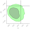 |
Fig. A.1. Localisation of GRB120711A with PySPI. Contours show the statistical only 1- and 2-sigma credible regions. We estimate an additional systematic error of ≈ 0.5 degrees because that is the resolution of the grid points in the response simulation. The dashed lines mark the position observed by Swift/XRT (Beardmore & Evans 2012). |
Appendix B: Model checking plots
In this section we show a selection of the PPC- and QQ-plots for the simultaneous synchrotron fit to the SPI and GBM data for GRB120711A.
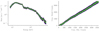 |
Fig. B.1. PPC (left) and QQ (right) plot for the GBM detector n0. The green and purple shaded areas are the one- and two-sigma contours. In the PPC plots, the dark yellow curve is the detected count spectrum, and in the QQ plots it shows the expected 1:1 relation between the cumulative model and observed counts. |
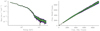 |
Fig. B.2. PPC (left) and QQ (right) plot for the GBM detector b0. The green and purple shaded area are the one- and two-sigma contours. The dark yellow curve has the same signification as in Fig. B.1. for the two plots. |
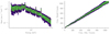 |
Fig. B.3. PPC (left) and QQ (right) plot for the low energy range of SPI detector 13 (all single events). The dark yellow curve has the same signification as in Fig. B.1. for the two plots. |
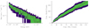 |
Fig. B.4. PPC (left) and QQ (right) plot for the middle energy range of SPI detector 13 (only PSD events). The dark yellow curve has the same signification as in Fig. B.1. for the two plots. |
All Figures
|
Fig. 1. Count spectrum for detector 0 integrated over 1000 s in revolution 1189. The non-PSD event count spectrum is drawn in purple and the PSD events in grey. The light green shaded area marks the energy range within the PSD energy thresholds (Roques & Jourdain 2019). The feature is clearly seen in the non-PSD events at 1.5 MeV (stronger green shaded area) and is not visible in the PSD events. |
| In the text | |
|
Fig. 2. Light curve for SPI detector 0 for GRB 120711A. The transient source is clearly visible as well as the constant background for the time when the transient is not active. The time interval we use for the independent background observation is marked with the green shaded area. |
| In the text | |
|
Fig. 3. Light curve for GRB 120711A in one GBM and one SPI detector. The green shaded area marks part of the time intervals used for the independent background observation and the blue shaded area is the active time interval used in the fit. |
| In the text | |
|
Fig. 4. Corner plot showing the Band function fit to the SPI data with PySPI and OSA with the data for GRB120711A. The results are in agreement, but PySPI constrains the parameters more precisely. |
| In the text | |
|
Fig. 5. Model posterior plots (95% confidence region) for the results with the Band function model and the data for GRB120711A. Left panel: results for the PySPI fit compared to the fit using OSA and right panel: PySPI fit compared to the GBM fit. |
| In the text | |
|
Fig. 6. Corner plot for the SPI fit with PySPI and the GBM fit to the data of GRB120711A. In this fit, we used a Band function as a spectral model. The spectral shapes for the SPI and GBM fits coincide within their uncertainty regions and the normalisation is off by ≈10%. |
| In the text | |
|
Fig. 7. Corner plot for the SPI fit with PySPI and the GBM fit to the data of GRB120711A. In this fit we used a physical synchrotron model (see Sect. 3) as a spectral model. The results from SPI and GBM agree within their uncertainty region and the combined fit provides better constraints on the parameter than the individual ones. |
| In the text | |
|
Fig. 8. Model posterior plots (95% confidence region) for the results with the physical synchrotron model and the data for GRB120711A. Left panel: results for the SPI fit compared to the combined fit and right panel: GBM fit compared to the combined fit. The combined fit reduces the allowed model space. |
| In the text | |
|
Fig. 9. Data (for GRB120711A) and best-fit model in count space for three of the SPI detectors and one of the NaI (BGO) detectors of GBM (upper and lower plot, respectively). The spectral model for this fit was a physical synchrotron model. |
| In the text | |
|
Fig. A.1. Localisation of GRB120711A with PySPI. Contours show the statistical only 1- and 2-sigma credible regions. We estimate an additional systematic error of ≈ 0.5 degrees because that is the resolution of the grid points in the response simulation. The dashed lines mark the position observed by Swift/XRT (Beardmore & Evans 2012). |
| In the text | |
|
Fig. B.1. PPC (left) and QQ (right) plot for the GBM detector n0. The green and purple shaded areas are the one- and two-sigma contours. In the PPC plots, the dark yellow curve is the detected count spectrum, and in the QQ plots it shows the expected 1:1 relation between the cumulative model and observed counts. |
| In the text | |
|
Fig. B.2. PPC (left) and QQ (right) plot for the GBM detector b0. The green and purple shaded area are the one- and two-sigma contours. The dark yellow curve has the same signification as in Fig. B.1. for the two plots. |
| In the text | |
|
Fig. B.3. PPC (left) and QQ (right) plot for the low energy range of SPI detector 13 (all single events). The dark yellow curve has the same signification as in Fig. B.1. for the two plots. |
| In the text | |
|
Fig. B.4. PPC (left) and QQ (right) plot for the middle energy range of SPI detector 13 (only PSD events). The dark yellow curve has the same signification as in Fig. B.1. for the two plots. |
| In the text | |
Current usage metrics show cumulative count of Article Views (full-text article views including HTML views, PDF and ePub downloads, according to the available data) and Abstracts Views on Vision4Press platform.
Data correspond to usage on the plateform after 2015. The current usage metrics is available 48-96 hours after online publication and is updated daily on week days.
Initial download of the metrics may take a while.