| Issue |
A&A
Volume 652, August 2021
|
|
|---|---|---|
| Article Number | A21 | |
| Number of page(s) | 15 | |
| Section | Cosmology (including clusters of galaxies) | |
| DOI | https://doi.org/10.1051/0004-6361/202140592 | |
| Published online | 03 August 2021 | |
Euclid : Effects of sample covariance on the number counts of galaxy clusters⋆
1
IFPU, Institute for Fundamental Physics of the Universe, Via Beirut 2, 34151 Trieste, Italy
e-mail: This email address is being protected from spambots. You need JavaScript enabled to view it.
2
Dipartimento di Fisica – Sezione di Astronomia, Universitá di Trieste, Via Tiepolo 11, 34131 Trieste, Italy
3
INAF-Osservatorio Astronomico di Trieste, Via G. B. Tiepolo 11, 34131 Trieste, Italy
4
INFN, Sezione di Trieste, Via Valerio 2, 34127 Trieste TS, Italy
5
Institute of Cosmology and Gravitation, University of Portsmouth, Portsmouth PO1 3FX, UK
6
INAF-Osservatorio di Astrofisica e Scienza dello Spazio di Bologna, Via Piero Gobetti 93/3, 40129 Bologna, Italy
7
INAF-Osservatorio Astronomico di Padova, Via dell’Osservatorio 5, 35122 Padova, Italy
8
Max Planck Institute for Extraterrestrial Physics, Giessenbachstr. 1, 85748 Garching, Germany
9
INAF-Osservatorio Astrofisico di Torino, Via Osservatorio 20, 10025 Pino Torinese (TO), Italy
10
INFN-Sezione di Roma Tre, Via della Vasca Navale 84, 00146 Roma, Italy
11
Department of Mathematics and Physics, Roma Tre University, Via della Vasca Navale 84, 00146 Rome, Italy
12
INAF-Osservatorio Astronomico di Roma, Via Frascati 33, 00078 Monteporzio Catone, Italy
13
Centro de Astrofísica da Universidade do Porto, Rua das Estrelas, 4150-762 Porto, Portugal
14
Instituto de Astrofísica e Ciências do Espaço, Universidade do Porto, CAUP, Rua das Estrelas, 4150-762 Porto, Portugal
15
INAF-IASF Milano, Via Alfonso Corti 12, 20133 Milano, Italy
16
Department of Physics “E. Pancini”, University Federico II, Via Cinthia 6, 80126 Napoli, Italy
17
INFN section of Naples, Via Cinthia 6, 80126 Napoli, Italy
18
INAF-Osservatorio Astronomico di Capodimonte, Via Moiariello 16, 80131 Napoli, Italy
19
INAF-Osservatorio Astrofisico di Arcetri, Largo E. Fermi 5, 50125 Firenze, Italy
20
Dipartimento di Fisica e Astronomia, Universitá di Bologna, Via Gobetti 93/2, 40129 Bologna, Italy
21
Institut national de physique nucléaire et de physique des particules, 3 rue Michel-Ange, 75794 Paris Cedex 16, France
22
Centre National d’Etudes Spatiales, Toulouse, France
23
Jodrell Bank Centre for Astrophysics, School of Physics and Astronomy, University of Manchester, Oxford Road, Manchester M13 9PL, UK
24
Aix-Marseille Univ, CNRS, CNES, LAM, Marseille, France
25
Mullard Space Science Laboratory, University College London, Holmbury St Mary, Dorking, Surrey RH5 6NT, UK
26
Department of Astronomy, University of Geneva, ch. d’Écogia 16, 1290 Versoix, Switzerland
27
Université Paris-Saclay, CNRS, Institut d’astrophysique spatiale, 91405 Orsay, France
28
INFN-Padova, Via Marzolo 8, 35131 Padova, Italy
29
Univ Lyon, Univ Claude Bernard Lyon 1, CNRS/IN2P3, IP2I Lyon, UMR 5822, 69622 Villeurbanne, France
30
Institute of Space Sciences (ICE, CSIC), Campus UAB, Carrer de Can Magrans, s/n, 08193 Barcelona, Spain
31
Institut d’Estudis Espacials de Catalunya (IEEC), Carrer Gran Capitá 2-4, 08034 Barcelona, Spain
32
INFN-Sezione di Bologna, Viale Berti Pichat 6/2, 40127 Bologna, Italy
33
Universitäts-Sternwarte München, Fakultät für Physik, Ludwig-Maximilians-Universität München, Scheinerstrasse 1, 81679 München, Germany
34
Dipartimento di Fisica “Aldo Pontremoli”, Universitá degli Studi di Milano, Via Celoria 16, 20133 Milano, Italy
35
INFN-Sezione di Milano, Via Celoria 16, 20133 Milano, Italy
36
INAF-Osservatorio Astronomico di Brera, Via Brera 28, 20122 Milano, Italy
37
Institute of Theoretical Astrophysics, University of Oslo, PO Box 1029 Blindern, 0315 Oslo, Norway
38
Leiden Observatory, Leiden University, Niels Bohrweg 2, 2333 CA Leiden, The Netherlands
39
Jet Propulsion Laboratory, California Institute of Technology, 4800 Oak Grove Drive, Pasadena, CA 91109, USA
40
von Hoerner & Sulger GmbH, SchloßPlatz 8, 68723 Schwetzingen, Germany
41
Max-Planck-Institut für Astronomie, Königstuhl 17, 69117 Heidelberg, Germany
42
AIM, CEA, CNRS, Université Paris-Saclay, Université Paris Diderot, Sorbonne Paris Cité, 91191 Gif-sur-Yvette, France
43
Université de Genève, Département de Physique Théorique and Centre for Astroparticle Physics, 24 quai Ernest-Ansermet, 1211 Genève 4, Switzerland
44
Department of Physics and Helsinki Institute of Physics, Gustaf Hällströmin katu 2, 00014 University of Helsinki, Finland
45
European Space Agency/ESTEC, Keplerlaan 1, 2201 AZ Noordwijk, The Netherlands
46
NOVA optical infrared instrumentation group at ASTRON, Oude Hoogeveensedijk 4, 7991 PD Dwingeloo, The Netherlands
47
Argelander-Institut für Astronomie, Universität Bonn, Auf dem Hügel 71, 53121 Bonn, Germany
48
Institute for Computational Cosmology, Department of Physics, Durham University, South Road, Durham DH1 3LE, UK
49
California institute of Technology, 1200 E California Blvd, Pasadena, CA 91125, USA
50
Observatoire de Sauverny, Ecole Polytechnique Fédérale de Lau- sanne, 1290 Versoix, Switzerland
51
INFN-Bologna, Via Irnerio 46, 40126 Bologna, Italy
52
Institut de Física d’Altes Energies (IFAE), The Barcelona Institute of Science and Technology, Campus UAB, 08193 Bellaterra, (Barcelona), Spain
53
Department of Physics and Astronomy, University of Aarhus, Ny Munkegade 120, 8000 Aarhus C, Denmark
54
Institute of Space Science, Bucharest 077125, Romania
55
I.N.F.N.-Sezione di Roma Piazzale Aldo Moro, 2 – c/o Dipartimento di Fisica, Edificio G. Marconi, 00185 Roma, Italy
56
Aix-Marseille Univ, CNRS/IN2P3, CPPM, Marseille, France
57
Dipartimento di Fisica e Astronomia “G. Galilei”, Universitá di Padova, Via Marzolo 8, 35131 Padova, Italy
58
Institute for Astronomy, University of Edinburgh, Royal Observatory, Blackford Hill, Edinburgh EH9 3HJ, UK
59
Instituto de Astrofísica e Ciências do Espaço, Faculdade de Ciências, Universidade de Lisboa, Tapada da Ajuda, 1349-018 Lisboa, Portugal
60
Departamento de Física, Faculdade de Ciências, Universidade de Lisboa, Edifício C8, Campo Grande, 1749-016 Lisboa, Portugal
61
Universidad Politécnica de Cartagena, Departamento de Electrónica y Tecnología de Computadoras, 30202 Cartagena, Spain
62
Kapteyn Astronomical Institute, University of Groningen, PO Box 800 9700 AV Groningen, The Netherlands
63
Infrared Processing and Analysis Center, California Institute of Technology, Pasadena, CA 91125, USA
64
European Space Agency/ESRIN, Largo Galileo Galilei 1, 00044 Frascati, Roma, Italy
65
ESAC/ESA, Camino Bajo del Castillo, s/n., Urb. Villafranca del Castillo, 28692 Villanueva de la Cañada, Madrid, Spain
66
APC, AstroParticule et Cosmologie, Université Paris Diderot, CNRS/IN2P3, CEA/lrfu, Observatoire de Paris, Sorbonne Paris Cité, 10 rue Alice Domon et Léonie Duquet, 75205 Paris Cedex 13, France
Received:
17
February
2021
Accepted:
9
April
2021
Abstract
Aims. We investigate the contribution of shot-noise and sample variance to uncertainties in the cosmological parameter constraints inferred from cluster number counts, in the context of the Euclid survey.
Methods. By analysing 1000 Euclid-like light cones, produced with the PINOCCHIO approximate method, we validated the analytical model of Hu & Kravtsov (2003, ApJ, 584, 702) for the covariance matrix, which takes into account both sources of statistical error. Then, we used such a covariance to define the likelihood function that is better equipped to extract cosmological information from cluster number counts at the level of precision that will be reached by the future Euclid photometric catalogs of galaxy clusters. We also studied the impact of the cosmology dependence of the covariance matrix on the parameter constraints.
Results. The analytical covariance matrix reproduces the variance measured from simulations within the 10 percent; such a difference has no sizeable effect on the error of cosmological parameter constraints at this level of statistics. Also, we find that the Gaussian likelihood with full covariance is the only model that provides an unbiased inference of cosmological parameters without underestimating the errors, and that the cosmology-dependence of the covariance must be taken into account.
Key words: galaxies: clusters: general / large-scale structure of Universe / cosmological parameters / methods: statistical
This paper is published on behalf of the Euclid Consortium.
© A. Fumagalli et al. 2021
 Open Access article, published by EDP Sciences, under the terms of the Creative Commons Attribution License (https://creativecommons.org/licenses/by/4.0), which permits unrestricted use, distribution, and reproduction in any medium, provided the original work is properly cited.
1. Introduction
Galaxy clusters are the most massive gravitationally bound systems in the Universe (M ∼ 1014 − 1015 M⊙) of which dark matter makes up about 85 percent, hot ionized gas 12 percent, and stars 3 percent (Pratt et al. 2019). These massive structures are formed by the gravitational collapse of initial perturbations of the matter density field via a hierarchical process of accreting and merging of small objects into increasingly massive systems (Kravtsov & Borgani 2012). Therefore galaxy clusters have several properties that can be used to obtain cosmological information on the geometry and the evolution of the large-scale structure of the Universe (LSS). In particular, the abundance and spatial distribution of such objects are sensitive to the variation of several cosmological parameters, such as the root mean square (RMS) mass fluctuation of the (linear) power spectrum on 8 h−1 Mpc scales (σ8) and the matter content of the Universe (Ωm) (Borgani et al. 1999; Schuecker et al. 2003; Allen et al. 2011; Pratt et al. 2019). Moreover, clusters can be observed at low redshift (out to redshift z ∼ 2), thus sampling the cosmic epochs during which the effect of dark energy begins to dominate the expansion of the Universe; as such, the evolution of the statistical properties of galaxy clusters should allow us to place constraints on the dark energy equation of state, and then detect possible deviations of dark energy from a simple cosmological constant (Sartoris et al. 2012). Finally, such observables can be used to constrain neutrino masses (e.g., Costanzi et al. 2013, 2019; Mantz et al. 2015; Bocquet et al. 2019; DES Collaboration 2020), the Gaussianity of initial conditions (e.g., Sartoris et al. 2010; Mana et al. 2013), and the behavior of gravity on cosmological scales (e.g., Cataneo & Rapetti 2018; Bocquet et al. 2015).
The main obstacle with regard to the use of clusters as cosmological probes lies in the proper calibration of systematic uncertainties involved in the analyses of cluster surveys. First, cluster masses are not directly observed but, instead, they must be inferred through other measurable properties of clusters, such as the properties of their galaxy population (i.e., richness, velocity dispersion) or of the intracluster gas (i.e., total gas mass, temperature, pressure). The relationships between these observables and clusters masses, referred to as scaling relations, provide a statistical measurement of masses, but require an accurate calibration in order to correctly relate the mass proxies with the actual cluster mass. Moreover, scaling relations can be affected by intrinsic scatter due to the properties of individual clusters and baryonic physics effects that complicate the calibration process (Kravtsov & Borgani 2012; Pratt et al. 2019). Other measurement errors are related to the estimation of redshifts and the selection function (Allen et al. 2011). In addition, there may be theoretical systematics related to modeling statistical errors: shot-noise, namely the uncertainty due to the discrete nature of the data, and sample variance, which is the uncertainty due to the finite size of the survey; in the case of a “full-sky” survey, the latter is referred to as the cosmic variance and it illustrates the fact that we are able to observe a single random realization of the Universe (e.g., Valageas et al. 2011). Finally, the analytical models describing the observed distributions, such as the mass function and halo bias, have to be carefully calibrated to avoid introducing further systematics (e.g., Sheth & Tormen 2002; Tinker et al. 2008, 2010; Bocquet et al. 2015; Despali et al. 2016; Castro et al. 2021).
The study and the control of these uncertainties are fundamental for future surveys, which will provide large cluster samples that will allow us to constrain cosmological parameters with a level of precision much higher than that obtained so far. One of the main forthcoming surveys is the European Space Agency (ESA) mission Euclid1, planned for 2022, which will map ∼15 000 deg2 of the extragalactic sky up to redshift 2 in order to investigate the nature of dark energy, dark matter, and gravity. Galaxy clusters are among the cosmological probes to be used by Euclid and the mission is expected to yield a sample of ∼105 clusters using photometric and spectroscopic data and through gravitational lensing (Laureijs et al. 2011; Euclid Collaboration 2019). A forecast of the capability of the Euclid cluster survey was performed by Sartoris et al. (2016), displaying the effect of the photometric selection function on the number of detected objects and the consequent cosmological constraints for different cosmological models. Also, Köhlinger et al. (2015) showed that weak lensing systematics in the mass calibration are under control for Euclid, as they will be limited by the cluster samples themselves.
The aim of this work is to assess the contribution of shot-noise and sample variance to the statistical error budget expected for the Euclid photometric survey of galaxy clusters. The expectation is that the level of shot-noise error would decrease due to the large number of detected clusters, making the sample variance no longer negligible. To quantify the contribution of these effects, an accurate statistical analysis is required, which is to be performed on a large number of realizations of past light cones extracted from cosmological simulations describing the distribution of cluster-sized halos. This is made possible using approximate methods for such simulations (e.g., Monaco 2016). A class of these methods describes the formation process of dark matter halos, that is, the dark matter component of galaxy clusters, through Lagrangian perturbation theory (LPT), which provides the distribution of large-scale structures in a faster and computationally less expensive way than through “exact” N-body simulations. As a disadvantage, such catalogs are less accurate and have to be calibrated to reproduce N-body results with sufficient precision. By using a large set of LPT-based simulations, we tested the accuracy of an analytical model for the computation of the covariance matrix and defined what the best likelihood function is for optimizing the extraction of unbiased cosmological information from cluster number counts. In addition, we also analyzed the impact of the cosmological dependence of the covariance matrix on the estimation of cosmological parameters.
This paper is organized as follows: in Sect. 2 we present the quantities involved in the analysis, such as the mass function, likelihood function, and covariance matrix. In Sect. 3 we describe the simulations used in this work, which are dark matter halo catalogs produced by the PINOCCHIO algorithm (Monaco et al. 2002; Munari et al. 2017). In Sect. 4, we present the analyses and the results that we obtained through a study of the number counts. In Sect. 4.1 (and in Appendix A), we validate the analytical model for the covariance matrix by comparing it with the matrix from the simulations. In Sect. 4.2, we analyze the effect of the mass and redshift binning on the estimation of parameters, while in Sect. 4.3 we compare the effect on the parameter posteriors of different likelihood models. In Sect. 5, we present our conclusions. While this paper is focused on the analysis relevant for a cluster survey similar in sky coverage and depth to that of Euclid , for completeness, we provide in Appendix B those results that are relevant for present and ongoing surveys.
2. Theoretical background
In this section, we introduce the theoretical framework needed to model the cluster number counts and derive cosmological constraints via Bayesian inference.
2.1. Number counts of galaxy clusters
The starting point for modeling the number counts of galaxy clusters is given by the halo mass function dn(M, z), defined as the comoving volume number density of collapsed objects at redshift z with masses between M and M + dM (Press & Schechter 1974),
 (1)
(1)
where  is the inverse of the Lagrangian volume of a halo of mass, M, and ν = δc/σ(R, z) is the peak height, defined in terms of the variance of the linear density field smoothed on a scale of R,
 (2)
(2)
where R is the radius enclosing the mass  , WR(k) is the filtering function, and P(k, z) the initial matter power spectrum, linearly extrapolated to redshift z. The term δc represents the critical linear overdensity for the spherical collapse and contains a weak dependence on cosmology and redshift that can be expressed as (Nakamura & Suto 1997):
![Mathematical equation: $$ \begin{aligned} \delta _{\rm c}(z) = \frac{3}{20} (12\pi )^{2/3} [1+0.012299 \mathrm{log}_{10}\Omega _{\rm m}(z)]\,. \end{aligned} $$](/articles/aa/full_html/2021/08/aa40592-21/aa40592-21-eq5.gif) (3)
(3)
One of the main characteristics of the mass function is that when it is expressed in terms of the peak height, its shape is nearly universal, meaning that the multiplicity function νf(ν) can be described in terms of a single variable and with the same parameters for all the redshifts and cosmological models (Sheth & Tormen 2002). A number of parametrizations have been derived by fitting the mass distribution from N-body simulations (Jenkins et al. 2001; White 2002; Tinker et al. 2008; Watson et al. 2013) in order to describe such universality with the highest possible degree of accuracy. At the present time, a fully universal parametrization has not yet been found and the main differences between the various results reside in the definition of halos, which can be based on the Friends-of-Friends (FoF) and Spherical Overdensity (SO) algorithms (e.g., White 2001; Kravtsov & Borgani 2012) or on the dynamical definition of the Splashback radius (Diemer 2017, 2020), as well as in the overdensity at which halos are identified. The need to improve the accuracy and precision in the mass function parametrization is reflected in the differences found in the cosmological parameter estimation, in particular, for future surveys such as Euclid (Salvati et al. 2020; Artis et al. 2021). Another way to predict the abundance of halos is the use of emulators, built by fitting the mass function from the simulations as a function of cosmology; such emulators are able to reproduce the mass function within an accuracy of a few percents (Heitmann et al. 2016; McClintock et al. 2019; Bocquet et al. 2020). The description of the cluster mass function is further complicated by the presence of baryons, which have to be taken into account when analyzing the observational data; their effect must therefore be included in the calibration of the model (e.g., Cui et al. 2014; Velliscig et al. 2014; Bocquet et al. 2015; Castro et al. 2021).
In this work, we fix the mass function assuming that the model has been correctly calibrated. The reference mass function that we assume for our analysis is given as (Despali et al. 2016, hereafter D16)2:
 (4)
(4)
with ν′ = aν2. The values of the parameters are: A = 0.3298, a = 0.7663, p = 0.2579 (“All z – Planck cosmology” case in D16). Comparisons with the numerical simulations show departures from the universality described by this model on the order of 5 − 8%, provided that halo masses are computed within the virial overdensity, as predicted by the spherical collapse model.
Besides the systematic uncertainty due to the fitting model, the mass function is affected by two sources of statistical error (which do not depend on the observational process): shot-noise and sample variance. Shot-noise is the sampling error that arises from the discrete nature of the data and contributes mainly to the high-mass tail of the mass function, where the number of objects is lower, being proportional to the square root of the number counts. On the other hand, sample variance depends only on the size and the shape of the sampled volume; it arises as a consequence of the existence of super-sample Fourier modes, with wavelengths exceeding the survey size, which cannot be sampled in the analyses of a finite volume survey. Sample variance introduces correlation between different mass and redshift ranges, unlike the shot-noise that only affects objects in the same bin. For data that is currently available, the main contribution to the error comes from shot-noise, while the sample variance term is usually neglected (e.g., Mantz et al. 2015; Bocquet et al. 2019). Nevertheless, upcoming and future surveys will provide catalogs with a larger number of objects, making the sample variance comparable, or even greater, than the shot-noise level (Hu & Kravtsov 2003). One example is provided by the Dark Energy Survey (DES Flaugher 2005), where the sample variance contribution is already taken into account when analyzing cluster number counts (DES Collaboration 2020; Costanzi et al. 2021).
2.2. Definition of likelihood functions
The analysis of the mass function was performed through Bayesian inference, by maximizing a likelihood function. The posterior distribution is explored with a Monte Carlo Markov chains (MCMC) approach (Heavens 2009), by using a python wrapper for the nested sampler qcrPyMultiNest (Buchner et al. 2014).
The likelihood commonly adopted in the literature for number counts analyses is the Poissonian one, which takes into account only the shot-noise term. To add the sample variance contribution, the simplest way is to use a Gaussian likelihood. In this work, we considered the following likelihood functions:
-
Poissonian:
 (5)
(5)where xiα and μiα are, respectively, the observed and expected number counts in the ith mass bin and αth redshift bin. Here, the bins are not correlated, since shot-noise does not produce cross-correlation, and the likelihoods are simply multiplied
-
Gaussian with shot-noise only:
 (6)
(6)where
 is the shot-noise variance. This function represents the limit of the Poissonian case for large occupancy numbers
 -
Gaussian with shot-noise and sample variance:
![Mathematical equation: $$ \begin{aligned} \mathcal{L} (x\,\vert \,\upmu ,\,C) = \frac{ \exp {\left\{ -\frac{1}{2} (\mathbf {x} -\boldsymbol{\upmu })^T C^{-1} (\mathbf {x} -\boldsymbol{\upmu }) \right\} }}{\sqrt{2\pi \det [C]}} \,, \end{aligned} $$](/articles/aa/full_html/2021/08/aa40592-21/aa40592-21-eq10.gif) (7)
(7)where x = {xiα} and μ = {μiα}, while C = {Cαβij} is the covariance matrix which correlates different bins due to the sample variance contribution. This function is also valid in the limit of large numbers, as the previous one.
We maximize the average likelihood, defined as
 (8)
(8)
where NS = 1000 is the number of light cones and lnℒ(a) is the likelihood of the a-th light-cone evaluated according to the equations described above. The posteriors obtained in this way are consistent with those of a single light cone but, in principle, centered on the input parameter values since the effect of cosmic variance that affects each realization of the matter density field is averaged-out when combining all the 1000 light cones; this procedure makes it easier to observe possible biases in the parameter posteriors due to the presence of systematics.
To estimate the differences on the parameter constraints between the various likelihood models, we quantify the cosmological gain using the figure of merit (FoM hereafter, Albrecht et al. 2006) in the Ωm – σ8 plane, defined as:
![Mathematical equation: $$ \begin{aligned} \mathrm{FoM} (\Omega _{\rm m}, \sigma _8) = \frac{1}{\sqrt{\det \left[ \mathrm{Cov} (\Omega _{\rm m}, \sigma _8) \right] }} \,, \end{aligned} $$](/articles/aa/full_html/2021/08/aa40592-21/aa40592-21-eq12.gif) (9)
(9)
where Cov(Ωm, σ8) is the parameter covariance matrix computed from the sampled points in the parameter space. The FoM is proportional to the inverse of the area enclosed by the ellipse representing the 68 percent confidence level and gives a measure of the accuracy of the parameter estimation: the larger the FoM, the more precise is the evaluation of the parameters. However, a larger FoM may not indicate a more efficient method of information extraction, but rather an underestimation of the error in the likelihood analysis.
2.3. Covariance matrix
The covariance matrix can be estimated from a large set of simulations through the equation:
 (10)
(10)
where m = 1, …, NS indicates the simulation,  is the number of objects in the ith mass bin and in the αth redshift bin for the mth catalog, while
  represents the same number averaged over the set of NS simulations. Such a matrix describes both the shot-noise variance, given simply by the number counts in each bin, and the sample variance contribution, or more aptly, the sample covariance:
 (11)
(11)
 (12)
(12)
In reality, the precision matrix C−1 (which has to be included in Eq. (7)) that is obtained by inverting Eq. (10) is biased due to the noise generated by the finite number of realizations; the inverse matrix must therefore be corrected by a factor (Anderson 2003; Hartlap et al. 2007; Taylor et al. 2013):
 (13)
(13)
where NS is the number of catalogs and ND the dimension of the data vector, that is, the total number of bins.
Although the use of simulations allows us to calculate the covariance in a simple way, numerical estimates of the covariance matrix have some limitations, mainly due to the presence of statistical noise which can only be reduced by increasing the number of catalogs. In addition, simulations make it possible to compute the matrix only at their input cosmology, preventing a fully cosmology-dependent analysis. To overcome these limitations, we can adopt an analytic prescription for the covariance matrix (Hu & Kravtsov 2003; Lacasa et al. 2018; Valageas et al. 2011). This involves a simplified treatment of non-linearities, so that the validity of this approach must be demonstrated by comparing it with the simulations. To this end, we consider the analytical model proposed by Hu & Kravtsov (2003) and validate its predictions against simulated data (see Sect. 4.1). As stated before, the total covariance is given by the sum of the shot-noise variance and the sample covariance,
 (14)
(14)
According to the model, such terms can be computed as:
 (15)
(15)
 (16)
(16)
where ⟨N⟩αi and ⟨Nb⟩αi are respectively the expectation values of number counts and number counts times the halo bias in the i-th mass bin and α-th redshift bin,
 (17)
(17)
 (18)
(18)
with Ωsky = 2π(1 − cos θ), where θ is the field-of-view angle of the light-cone, and b(M, z) represents the halo bias as a function of mass and redshift. In the following, we adopt for the halo bias the expression provided by Tinker et al. (2010). The term Sαβ is the covariance of the linear density field between two redshift bins,
 (19)
(19)
where D(z) is the linear growth rate, P(k) is the linear matter power spectrum at the present time, and Wα(k) is the window function of the redshift bin, which depends on the shape of the volume probed. The simplest case is the spherical top-hat window function (see Appendix A), while the window function for a redshift slice of a light-cone is given in Costanzi et al. (2019) and takes the form:
![Mathematical equation: $$ \begin{aligned} W_{\alpha }(\boldsymbol{k}) = \frac{4\pi }{V_{\alpha }} \int _{\Delta z_{\alpha }} \mathrm{d}z \;\frac{\mathrm{d}V}{\mathrm{d}z} \sum _{\ell =0}^{\infty } \sum _{m = -\ell }^{\ell } (\mathrm{i})^\ell \,j_\ell [k\,r(z)] \,Y_{\ell m}(\hat{\boldsymbol{k}}) \,K_\ell \,, \end{aligned} $$](/articles/aa/full_html/2021/08/aa40592-21/aa40592-21-eq25.gif) (20)
(20)
where dV/dz and Vα are, respectively, the volume per unit redshift and the volume of the slice, which depend on cosmology. Also, in the above equation, jℓ[k r(z)] are the spherical Bessel functions,  are the spherical harmonics,
  is the angular part of the wave-vector, and Kℓ are the coefficients of the harmonic expansion, such that
where Pℓ(cos θ) are the Legendre polynomials.
3. Simulations
The accurate estimation of the statistical uncertainty associated with number counts must be carried out with a large set of simulated catalogs representing different realizations of the Universe. Such a large number of synthetic catalogs can hardly be provided by N-body simulations, which are capable of producing accurate results but have high computational costs. Instead, the use of approximate methods, based on perturbative theories, makes it possible to generate a large number of catalogs in a faster and far less computationally expensive way compared to N-body simulations. This comes at the expense of less accurate results: perturbative theories give an approximate description of particle and halo displacements that are computed directly from the initial configuration of the gravitational potential, rather than by computing the gravitational interactions at each time step of the simulation (e.g., Monaco 2016; Sahni & Coles 1995).
PINOCCHIO (PINpointing Orbit-Crossing Collapsed HIerarchical Objects; Monaco et al. 2002; Munari et al. 2017) is an algorithm that generates dark matter halo catalogs through LPT (Moutarde et al. 1991; Buchert 1992; Bouchet et al. 1995) and ellipsoidal collapse (e.g. Bond & Myers 1996; Eisenstein & Loeb 1995) up to the third order. The code simulates cubic boxes with periodic boundary conditions, starting from a regular grid on which an initial density field is generated in the same way as in N-body simulations. A collapse time is computed for each particle using ellipsoidal collapse. The collapsed particles on the grid are then displaced with LPT to form halos, and halos are finally moved to their final positions by again applying the LPT. The code is also able to build past light cones (PLC), by replicating the periodic boxes through an “on-the-fly” process that selects only the halos causally connected with an observer at the present time, once the position of the “observer” and the survey sky area are fixed. This method permits us to generate PLC in a continuous way, that is, avoiding the “piling-up” snapshots at a discrete set of redshifts.
The catalogs generated by PINOCCHIO are able to reproduce, within a ∼5 − 10 percent accuracy, the two-point statistics on large scales (k < 0.4 h Mpc−1), as well as the linear bias and the mass function of halos derived from full N-body simulations (Munari et al. 2017). The accuracy of these statistics can be further increased by re-scaling the PINOCCHIO halo masses in order to match a specific mass function calibrated against N-body simulations.
We analyzed 1000 past light cones3 with aperture of 60°, that is, a quarter of the sky, starting from a periodic box of size L = 3870 h−1 Mpc4. The light cones cover a redshift range from z = 0 to z = 2.5 and contain halos with virial masses above 2.45 × 10¹³ h−1 M⊙, sampled with more than 50 particles. The cosmology used in the simulations comes from Planck Collaboration XVI (2014): Ωm = 0.30711, Ωb = 0.048254, h = 0.6777, ns = 0.96, σ8 = 0.8288.
Before starting our analysis of the catalogs, we performed a calibration of the halo masses. This step is required both because the PINOCCHIO accuracy in reproducing the halo mass function is “only” 5 percent, and because its calibration is performed by considering a universal FoF halo mass function, whereas D16 define halos based on spherical overdensity within the virial radius, demonstrating that the resulting mass function is much nearer to a universal evolution than that of FoF halos.
Masses were re-scaled by matching the halo mass function of the PINOCCHIO catalogs to the analytical model of D16. In particular, we predicted the value for each single mass Mi by using the cumulative mass function:
 (21)
(21)
where i = 1, 2, 3…; and we assigned such values to the simulated halos, previously sorted by preserving the mass order ranking. During this process, all the thousand catalogs were stacked together, which is equivalent to using a 1000 times larger volume: the mean distribution obtained in this way contains fluctuations due to shot-noise and sample variance that are reduced by a factor of  and can thus be properly compared with the theoretical one, preserving the fluctuations in each rescaled catalog. Otherwise, if the mass function from each single realization was directly compared with the model, the shot-noise and sample variance effects would have been washed away.
In our analyses, we considered objects in the mass range 1014 ≤ M/M⊙ ≤ 1016 and redshift range 0 ≤ z ≤ 2; in this interval, each rescaled light-cone contains ∼3 × 10⁵ halos. We note that this simple constant mass-cut at 1014 M⊙ provides a reasonable approximation to a more refined computation of the mass selection function expected for the Euclid photometric survey of galaxy clusters (see Fig. 2 of Sartoris et al. 2016; see also Euclid Collaboration 2019).
In Fig. 1, we show the comparison between the calibrated and non-calibrated mass function of the light cones, averaged over the 1000 catalogs, in the redshift bin z = 0.1–0.2. For a better comparison, in the bottom panel we show the residual between the two mass functions from simulations and the one of D16: while the original distribution clearly differs from the analytical prediction, the calibrated mass function follows the model at all masses, except for some small fluctuations in the high-mass end where the number of objects per bin is low.
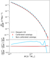 |
Fig. 1. Halo mass function for the mass calibration of the PINOCCHIO catalogs. Top panel: comparison between the mass function from the calibrated (red) and the non-calibrated (blue) light cones, averaged over the 1000 catalogs, in the redshift bin z = 0.1 − 0.2. Error bars represent the standard error on the mean. The black line is the D16 mass function. Bottom panel: relative difference between the mass function from simulations and that of D16. |
We also tested the model for the halo bias of Tinker et al. (2010, hereafter T10) to understand if the analytical prediction is in agreement with the bias from the rescaled catalogs. The latter is computed by applying the definition
 (22)
(22)
where ξm is the linear two-point correlation function (2PCF) for matter and ξh is the 2PCF for halos with masses above a threshold M; we use 10 mass thresholds in the range 1014 ≤ M/M⊙ ≤ 1015. We compute the correlation functions in the range of separations r = 30 − 70 h−1 Mpc, where the approximation of scale-independent bias is valid (Manera & Gaztañaga 2011). The error is computed by propagating the uncertainty in ξh, which is an average over the 1000 light cones. Since the bias from simulations refers to halos with mass ≥M, the comparison with the T10 model must be made with an effective bias, that is, a cumulative bias weighted on the mass function:
 (23)
(23)
Such a comparison is shown in Fig. 2, representing the effective bias from boxes at various redshifts and the corresponding analytical model, as a function of the peak height (the relation with mass and redshift is shown in Sect. 2.1). We notice that the T10 model slightly overestimates (underestimates) the simulated data at low (high) masses and redshifts: the difference is below the 5 percent level over the whole ν range, except for high-ν halos, where the discrepancy is about 10 percent. At low redshift, this difference is not compatible with the error on the measurements; however, such errors underestimate the real uncertainty, as they do not take into account the correlation between radial bins. We conclude that the T10 model can provide a sufficiently accurate prediction for the halo bias of our simulations.
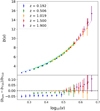 |
Fig. 2. Comparison between the T10 halo bias and the bias from the simulations. Top panel: halo bias from simulations at different redshifts (colored dots), compared to the analytical model of T10 (lighter solid lines). Bottom panel: fractional differences between the bias from simulations and from the model. |
4. Results
In this section, we present the results of the covariance comparison and likelihood analyses. First, we validated the analytical covariance matrix, described in Sect. 2.3, comparing it with the matrix from the mocks; this allows us to determine whether the analytical model correctly reproduces the results of the simulations. Once we verified that we had a correct description of the covariance, we moved on to the likelihood analysis. First, we analyzed the optimal redshift and mass binning scheme, which ensures that we extract the cosmological information in the best possible way. Then, after fixing the mass and redshift binning scheme, we tested the effects on parameter posteriors of different model assumptions: likelihood model and the inclusion of sample variance and cosmology dependence.
With the likelihood analysis, we aim to correctly recover the input values of the cosmological parameters Ωm, σ8 and log10 As. We directly constrain Ωm and log10 As, assuming flat priors in 0.2 ≤ Ωm ≤ 0.4 and −9.0 ≤ log10 As ≤ − 8.0, and then derive the corresponding value of σ8; thus, σ8 and log10 As are redundant parameters, linked by the relation P(k) ∝ As kns and by Eq. (2). All the other parameters are set to the Planck 2014 values. We are interested in detecting possible effects on the results that can occur, in principle, both in terms of biased parameters and over- or underestimating the parameter errors. The former case indicates the presence of systematics due to an incorrect analysis, while the latter suggests that not all the relevant sources of error have been taken into account.
4.1. Covariance matrix estimation
As we mentioned before, the sample variance contribution to the noise can be included in the estimation of cosmological parameters by computing a covariance matrix that takes into account the cross-correlation between objects in different mass or redshift bins. We computed the matrix in the range of 0 ≤ z ≤ 2 with Δz = 0.1 and 1014 ≤ M/M⊙ ≤ 1016. According to Eq. (13), since we used NS = 1000 and ND = 100 (20 redshift bins and 5 log-equispaced mass bins), we must correct the precision matrix by a factor of 0.90.
In the left panel of Fig. 3, we show the normalized sample covariance matrix, obtained from simulation, which is defined as the relative contribution of the sample variance with respect to the shot-noise level,
 (24)
(24)
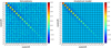 |
Fig. 3. Normalized sample covariance between redshift and mass bins (Eq. (24)), from simulations (left) and analytical model (right). The matrices are computed in the redshift range 0 ≤ z ≤ 1 with Δz = 0.2 and the mass range 1014 ≤ M/M⊙ ≤ 1016, divided into five bins. Black lines denote the redshift bins, while in each black square, there are different mass bins. |
where CSN and CSV are computed from Eqs. (11) and (12). The correlation induced by the sample variance is clearly detected in the block-diagonal covariance matrix (i.e., between mass bins), at least in the low-redshift range where the sample variance contribution is comparable to, or even greater than the shot-noise level. Instead, the off-diagonal and the high-redshift diagonal terms appear affected by the statistical noise mentioned in Sect. 2.3, which completely dominates over the weak sample variance (anti-)correlation.
In the right panel of Fig. 3, we show the same matrix computed with the analytical model: by comparing the two results, we note that the covariance matrix derived from simulations is well reproduced by the analytical model, at least for the diagonal and the first off-diagonal terms, where the former is not dominated by the statistical noise. To ease the comparison between simulations and model and between the amount of correlation of the various components, in Fig. 4 we show the covariance from model and simulations for different terms and components of the matrix, as a function of redshift: in blue we show the sample variance diagonal terms (i.e., same mass and redshift bin,  ), in red and orange the diagonal sample variance in two different mass bins (
 with respectively j = i + 1 and j = i + 2), in green the sample variance between two adjacent redshift bins (
 ), and in gray the shot-noise variance (
 ). In the upper panel, we show the full covariance, in the central panel the covariance normalized as in Eq. (24) and in the lower panel the normalized difference between model and simulations. Confirming what was noticed from Fig. 3, the block-diagonal sample variance terms are the dominant sources of error at low redshift, with a signal that rapidly decreases when considering different mass bins (blue, red, and orange lines), while shot-noise dominates at high redshift. We also observe that the cross-correlation between different redshift bins produces a small anti-correlation, whose relevance, however, seems negligible; further considerations about this point are presented in Sect. 4.3.
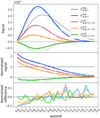 |
Fig. 4. Covariance (upper panel) and covariance normalized to the shot-noise level (central panel) as predicted by the Hu & Kravtsov (2003) analytical model (solid lines) and by simulations (dashed lines) for different matrix components: diagonal sample variance terms in blue, diagonal sample variance terms in two different mass bins in red and orange, sample variance between two adjacent redshift bins in green and shot-noise in gray. Lower panel: relative difference between analytical model and simulations. The curves are represented as a function of redshift, in the first mass bin (i = 1). |
Regarding the comparison between model and simulations, the figure clearly shows that the analytical model reproduces with good agreement the covariance from simulations, with deviations within 10 percent. Such agreement was expected, as the modes responsible for the sample covariance are generally very large, well within the linear regime in which the model operates. Part of the difference can be ascribed to the statistical noise, which produces random fluctuations in the simulated covariance matrix. We also observe, mainly on the block-diagonal terms, a slight underestimation of the correlation at low redshift and a small overestimation at high redshift, which are consistent with the under- and overestimation of the T10 halo bias, shown in Fig. 2. Additional analyses are presented in Appendix A, where we treat the description of the model with a spherical top-hat window function. Nevertheless, this discrepancy on the covariance errors has negligible effects on the parameter constraints, at this level of statistics. This comparison will be further analyzed in Sect. 4.3.
4.2. Redshift and mass binning
The optimal binning scheme should ensure to extract the maximum information from the data while avoiding the waste of computational resources with an exceedingly fine binning: adopting too large bins would hide some information, while too small bins can saturate the extractable information, making the analyses unnecessarily computationally expensive. Such saturation occurs even earlier when considering the sample covariance, which strongly correlates narrow mass bins. Moreover, too narrow bins could undermine the validity of the Gaussian approximation due to the low occupancy numbers. This can happen also at high redshift, where the number density of halos drops fast.
To establish the best binning scheme for the Poissonian likelihood function, we analyze the data, assuming four redshift bin widths Δz = {0.03, 0.1, 0.2, 0.3} and three numbers of mass bins NM = {50, 200, 300}. In Fig. 5 we show the FoM as a function of Δz, for different mass binning. Since each result of the likelihood maximization process is affected by some statistical noise, the points represent the mean values obtained from five realizations (which are sufficient for a consistent average result), with the corresponding standard error. About the redshift binning, the curve increases with decreasing Δz and flattens below Δz ∼ 0.2; from this result we conclude that for bin widths ≲0.2 the information is fully preserved and, among these values, we choose Δz = 0.1 as the bin width that maximize the information. The change of the mass binning affects the results in a minor way, giving points that are consistent with each other for all the redshift bin widths. To better study the effect of the mass binning, we compute the FoM also for NM = {5, 500, 600} at Δz = 0.1, finding that the amount of recovered information saturates around NM = 300. Thus, we use NM = 300 for the Poissonian likelihood case, corresponding to Δlog10(M/M⊙) = 0.007.
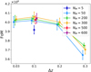 |
Fig. 5. Figure of merit for the Poissonian likelihood as a function of the redshift bin widths, for different numbers of mass bins. The points represent the average value over five realizations and the error bars are the standard error of the mean. A small horizontal offset has been applied to make the comparison clearer. |
We repeat the analysis for the Gaussian likelihood (with full covariance), by considering the redshift bin widths Δz = {0.1, 0.2, 0.3} and three numbers of mass bins NM = {5, 7, 10}, plus NM = {2, 20} for Δz = 0.1. We do not include the case of a tighter redshift or mass binning, to avoid deviating too much from the Gaussian limit of large occupancy numbers. The result for the FoM is shown Fig. 6, from which we can state that also for the Gaussian case the curve starts to flatten around Δz ∼ 0.2 and Δz = 0.1 results to be the optimal redshift binning, since for larger bin widths less information is extracted and for tighter bins the number of objects becomes too low for the validity of the Gaussian limit. Also in this case the mass binning does not influence the results in a significant way, provided that the number of binning is not too low. We chose to use NM = 5, corresponding to the mass bin widths Δlog10(M/M⊙) = 0.4.
4.3. Likelihood comparison
In this section, we present the comparison between the posteriors of cosmological parameters obtained by applying the different definitions of likelihood results on the entire sample of light cones, by considering the average likelihood defined by Eq. (8).
The first result is shown in Fig. 7, which represents the posteriors derived from the three likelihood functions: Poissonian, Gaussian with only shot-noise and Gaussian with shot-noise and sample variance (Eqs. (5)–(7), respectively). For the latter, we compute the analytical covariance matrix at the input cosmology and compare it with the results obtained by using the covariance matrix from simulations. The corresponding FoM in the σ8 – Ωm plane is shown in Fig. 8. The first two cases look almost the same, meaning that a finer mass binning as the one adopted in the Poisson likelihood does not improve the constraining power compared to the results from a Gaussian plus shot-noise covariance. In contrast, the inclusion of the sample covariance (blue and black contours) produces wider contours (and smaller FoM), indicating that neglecting this effect leads to an underestimation of the error on the parameters. Also, there is no significant difference in using the covariance matrix from the simulations or the analytical model, since the difference in the FoM is below the level of one percent. This result means that the level of accuracy reached by the model is sufficient to obtain an unbiased estimation of parameters in a survey of galaxy clusters having sky coverage and cluster statistics comparable to that of the Euclid survey. According to this conclusion, we can use the analytical covariance matrix to describe the statistical errors for all following likelihood evaluations.
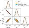 |
Fig. 7. Contour plots at 68 and 95 per cent of confidence level for the three likelihood functions: Poissonian (red), Gaussian with only shot-noise (orange) and Gaussian with shot-noise and sample variance, with covariance from the analytical model (blue) and from simulations (black). The gray dotted lines represent the input values of parameters. |
Having established that the inclusion of the sample variance has a non-negligible effect on parameter posteriors, we focus on the Gaussian likelihood case. In Fig. 9, we show the results obtained by using the full covariance matrix and only the block-diagonal of such a matrix (Cijαα), namely by considering shot-noise and sample variance effects between masses at the same redshift but with no correlation between different redshift bins. The resulting contours present small differences, as can be seen from the comparison of the FoM in Fig. 8: the difference in the FoM between the diagonal and full covariance cases is about one third of the effect generated by the inclusion of the full covariance with respect the only shot-noise cases. This means that at this level of statistics and for this redshift binning, the main contribution to the sample covariance comes from the correlation between mass bins, while the correlation between redshift bins produces a minor effect on the parameter posteriors. However, the difference between the two FoMs is not necessarily negligible: for three parameters, a ∼25% change in the FoM corresponds to a potential underestimate of the parameter errorbar by ∼10%. The Euclid Consortium is presently requiring that for the likelihood estimation, approximations should introduce a bias in parameter errorbars that is smaller than 10%, so as not to impact the first significant digit of the error. Because the list of potential systematics at the required precision level is long, it is necessary to avoid any oversimplification that would alone induce such a sizeable effect. The full covariance is thus required to properly describe the sample variance effect at the Euclid level of accuracy.
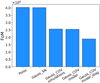 |
Fig. 8. Figure of merit for the different likelihood models: Poissonian, Gaussian with shot-noise, Gaussian with full covariance from simulations, Gaussian with full covariance from the model and Gaussian with block-diagonal covariance from the model. |
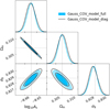 |
Fig. 9. Contour plots at 68 and 95 per cent of confidence level for the Gaussian likelihood with full covariance (blue) and the Gaussian likelihood with block-diagonal covariance (black). The gray dotted lines represent the input values of parameters. |
4.4. Cosmology dependence of covariance
We also investigate if there are differences in using a cosmology-dependent covariance matrix instead of a cosmology-independent one. In fact, the use of a matrix evaluated at a fixed cosmology can represent an advantage by reducing the computational cost, but may bias the results. In Fig. 10, we compare the parameters estimated with a cosmology-dependent covariance (black contours), namely, by recomputing the covariance at each step of the MCMC process, with the posteriors obtained by evaluating the matrix at the input cosmology (blue), or assuming a slightly lower or higher value for Ωm, log10 As and σ8 (red and orange contours, respectively), chosen on the basis of their departures from the fiducial values of the order of 2σ from Planck Collaboration VI (2020). Specifically, we fix the parameter values at Ωm = 0.295, log10 As = −8.685 and σ8 = 0.776 for the lower case and Ωm = 0.320, log10 As = −8.625 and σ8 = 0.884 for the higher case. We notice, also from the FoM comparison in Fig. 11, that there is no appreciable difference between the first two cases. In contrast, when a wrong-cosmology covariance matrix is used we can find either tighter or wider contours, meaning that the effect of shot-noise and sample variance can be either under- or overestimated. Thus, the use of a cosmology-independent covariance matrix in the analysis of real cluster abundance data might lead to under- or overestimated parameter uncertainties at the level of statistic expected for Euclid. On the contrary, the use of a cosmology-dependent covariance does not affect the amount of information obtainable from the data compared to the input-cosmology case. An alternative way to include the cosmology dependence of the covariance is to perform an iterative likelihood analysis, in which a cosmology-independent covariance is updated in every iteration according to the maximum likelihood cosmology retrieved in the previous step (Eifler et al. 2009).
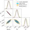 |
Fig. 10. Contour plots at the 68 and 95 percent confidence levels for the Gaussian likelihood evaluated with: a cosmology-dependent covariance matrix (black), a covariance matrix fixed at the input cosmology (blue) and covariance matrices computed at two wrong cosmologies, one with lower parameter values (Ωm = 0.295, log10 As = −8.685 and σ8 = 0.776, red) and one with higher parameter values (Ωm = 0.320, log10 As = −8.625 and σ8 = 0.884, orange). The gray dotted lines represent the input values of parameters. |
5. Discussion and conclusions
In this work, we study some of the theoretical systematics that can affect the derivation of cosmological constraints from the analysis of number counts of galaxy clusters from a survey with its sky-coverage and selection function similar to what is expected for the photometric Euclid cluster survey. One of the aims of the paper was to understand whether the inclusion of sample variance, in addition to the shot-noise error, could have some influence on the estimation of cosmological parameters at the level of statistics that will be reached by the future Euclid catalogs. We note that in this work we only consider uncertainties that do are not related directly to the observations, thus neglecting the systematics related to the mass estimation; however Köhlinger et al. (2015) state that for Euclid, the mass estimates from weak lensing would be under control and, although there would still be additional statistical and systematic uncertainties due to mass calibration, the analysis of real catalogs will approach the ideal case considered here.
To describe the contribution of shot-noise and sample variance, we computed an analytical model for the covariance matrix, representing the correlation between mass and redshift bins as a function of cosmological parameters. Once the model for the covariance has been properly validated, we moved to the identification of the more appropriate likelihood function to analyze cluster abundance data. The likelihood analysis has been performed with only two free parameters, Ωm and log10 As (and thus σ8), since the mass function is less affected by the variation of the other cosmological parameters.
Both the validation of the analytical model for the covariance matrix and the comparison between posteriors from different likelihood definitions are based on the analysis of an extended set of 1000 Euclid-like past light cones generated with the LPT-based PINOCCHIO code (Monaco et al. 2002; Munari et al. 2017).
The main results of our analysis can be summarized as follows.
-
To include the sample variance effect in the likelihood analysis, we computed the covariance matrix from a large set of mock catalogs. Most of the sample variance signal is contained in the block-diagonal terms of the matrix, giving a contribution larger than the shot-noise term, at least in the low-mass and low-redshift regime. On the other hand, the anti-correlation between different redshift bins produces a minor effect with respect to the diagonal variance.
-
We computed the covariance matrix by applying the analytical model by Hu & Kravtsov (2003), assuming the appropriate window function, and verified that it reproduces the matrix from simulations with deviations below the 10 percent level accuracy; this difference can be ascribed mainly to the non-perfect match of the T10 halo bias with the one from simulations. However, we verified that such a small difference does not affect the inference of cosmological parameters in a significant way, at the level of statistic of the Euclid survey. Therefore, we conclude that the analytical model of Hu & Kravtsov (2003) can be reliably applied to compute a cosmology-dependent, noise-free covariance matrix, without requiring a large number of simulations.
-
We established the optimal binning scheme to extract the maximum information from the data, while limiting the computational cost of the likelihood estimation. We analyzed the halo mass function with a Poissonian and a Gaussian likelihood, for different redshift- and mass-bin widths and then computed the figure of merit from the resulting contours in Ωm – σ8 plane. The results show that for both the Poissonian and the Gaussian likelihood, the optimal redshift bin width is Δz = 0.1: for larger bins, not all the information is extracted; while for smaller bins, the Poissonian case saturates and the Gaussian case is no longer a valid approximation. The mass binning affects less the results, provided an overly low number of bins is not selected. We decided to use NM = 300 for the Poissonian likelihood and NM = 5 for the Gaussian case.
-
We included the covariance matrix in the likelihood analysis and demonstrated that the contribution to the total error budget and the correlation induced by the sample variance term cannot be neglected. In fact, the Poissonian and Gaussian with shot-noise likelihood functions show smaller errorbars with respect to the Gaussian with covariance likelihood, meaning that neglecting the sample covariance leads to an underestimation of the error on parameters, at the Euclid level of accuracy. As shown in Appendix B, this result holds also for the eROSITA survey, whereas it is not valid for present surveys like Planck and SPT.
-
We verified that the anti-correlation between bins at different redshifts produces a minor, but non-negligible effect on the posteriors of cosmological parameters at the level of statistics reached by the Euclid survey. We also established that a cosmology-dependent covariance matrix is more appropriate than the cosmology-independent case, which can lead to biased results due to the wrong quantification of shot-noise and sample variance.
One of the main results of the analysis presented here is that for the next generation surveys of galaxy clusters, such as Euclid, sample variance effects need to be properly included, as they are being shown as one of the main sources of statistical uncertainty in the cosmological parameters estimation process. The correct description of sample variance is guaranteed by the analytical model validated in this work.
This analysis represents the first step toward providing all the necessary ingredients for an unbiased estimation of cosmological parameters from the number counts of galaxy clusters. It has to be complemented with the characterization of the other theoretical systematics, for instance, one that is related to the calibration of the halo mass function, and observational systematics related to the mass-observable relation and to the cluster selection function.
To further improve the extractable information from galaxy clusters, the same analysis will be extended to the clustering of galaxy clusters by analyzing the covariance of the power spectrum or of the two-point correlation function. Once all the systematics are calibrated, so as to properly combine two such observables (Schuecker et al. 2003; Mana et al. 2013; Lacasa & Rosenfeld 2016), number counts and clustering of galaxy clusters will provide valuable observational constraints, complementary to those of the other two main Euclid probes, namely, galaxy clustering and cosmic shear.
In D16, the peak height is defined as  ; in such cases, the factor of “2” in Eq. (4) disappears.
The PLC can be obtained on request. The list of the available mocks can be found at http://adlibitum.oats.inaf.it/monaco/mocks.html; the light cones analyzed are the ones labeled “NewClusterMocks”.
The Euclid light cones will be slightly larger than our simulations (about a third of the sky); moreover the survey will cover two separate patches of the sky, which is relevant to the effect of sample variance. However, for this first analysis, the PINOCCHIO light cones are sufficient to obtain an estimate of the statistical error that will characterize catalogs of such sizes and number of objects.
Masses in the paper are defined at the overdensity Δ = 500 with respect to the critical density; the conversion to virial masses has been performed with the python package qcrhydro_mc (https://github.com/aragagnin/hydro_mc).
Acknowledgments
We would like to thank Laura Salvati for useful discussions about the selection functions. SB, AS and AF acknowledge financial support from the ERC-StG ‘ClustersxCosmo’ grant agreement 716762, the PRIN-MIUR 2015W7KAWC grant, the ASI-Euclid contract and the INDARK grant. TC is supported by the INFN INDARK PD51 grant and by the PRIN-MIUR 2015W7KAWC grant. Our analyses have been carried out at: CINECA, with the projects INA17_C5B32 and IsC82_CosmGC; the computing center of INAF-Osservatorio Astronomico di Trieste, under the coordination of the CHIPP project (Bertocco et al. 2019; Taffoni et al. 2020). The Euclid Consortium acknowledges the European Space Agency and a number of agencies and institutes that have supported the development of Euclid, in particular the Academy of Finland, the Agenzia Spaziale Italiana, the Belgian Science Policy, the Canadian Euclid Consortium, the Centre National d’Etudes Spatiales, the Deutsches Zentrum für Luft- und Raumfahrt, the Danish Space Research Institute, the Fundação para a Ciência e a Tecnologia, the Ministerio de Economia y Competitividad, the National Aeronautics and Space Administration, the Netherlandse Onderzoekschool Voor Astronomie, the Norwegian Space Agency, the Romanian Space Agency, the State Secretariat for Education, Research and Innovation (SERI) at the Swiss Space Office (SSO), and the United Kingdom Space Agency. A complete and detailed list is available on the Euclid website (http://www.euclid-ec.org).
References
- Albrecht, A., Bernstein, G., Cahn, R., et al. 2006, ArXiv e-prints [arXiv:0609591] [Google Scholar]
- Allen, S. W., Evrard, A. E., & Mantz, A. B. 2011, ARA&A, 49, 409 [NASA ADS] [CrossRef] [Google Scholar]
- Anderson, T. 2003, An Introduction to Multivariate Statistical Analysis, Wiley Series in Probability and Statistics (Wiley) [Google Scholar]
- Artis, E., Melin, J.-B., Bartlett, J. G., & Murray, C. 2021, A&A, 649, A47 [CrossRef] [EDP Sciences] [Google Scholar]
- Bertocco, S., Goz, D., Tornatore, L., et al. 2019, ArXiv e-prints [arXiv:1912.05340] [Google Scholar]
- Bocquet, S., Saro, A., Mohr, J. J., et al. 2015, ApJ, 799, 214 [NASA ADS] [CrossRef] [Google Scholar]
- Bocquet, S., Saro, A., Dolag, K., & Mohr, J. J. 2016, MNRAS, 456, 2361 [Google Scholar]
- Bocquet, S., Dietrich, J. P., Schrabback, T., et al. 2019, ApJ, 878, 55 [NASA ADS] [CrossRef] [Google Scholar]
- Bocquet, S., Heitmann, K., Habib, S., et al. 2020, ApJ, 901, 5 [CrossRef] [Google Scholar]
- Bond, J. R., & Myers, S. T. 1996, ApJS, 103, 1 [NASA ADS] [CrossRef] [Google Scholar]
- Borgani, S., Plionis, M., & Kolokotronis, E. 1999, MNRAS, 305, 866 [NASA ADS] [CrossRef] [Google Scholar]
- Bouchet, F. R., Colombi, S., Hivon, E., & Juszkiewicz, R. 1995, A&A, 296, 575 [NASA ADS] [Google Scholar]
- Buchert, T. 1992, MNRAS, 254, 729 [NASA ADS] [CrossRef] [Google Scholar]
- Buchner, J., Georgakakis, A., Nandra, K., et al. 2014, A&A, 564, A125 [NASA ADS] [CrossRef] [EDP Sciences] [Google Scholar]
- Carlstrom, J. E., Ade, P. A. R., Aird, K. A., et al. 2011, PASP, 123, 568 [NASA ADS] [CrossRef] [Google Scholar]
- Castro, T., Borgani, S., Dolag, K., et al. 2021, MNRAS, 500, 2316 [Google Scholar]
- Cataneo, M., & Rapetti, D. 2018, Int. J. Mod. Phys. D, 27, 1848006 [CrossRef] [Google Scholar]
- Costanzi, M., Sartoris, B., Xia, J.-Q., et al. 2013, J. Cosmol. Astropart. Phys., 2013, 020 [NASA ADS] [CrossRef] [Google Scholar]
- Costanzi, M., Rozo, E., Simet, M., et al. 2019, MNRAS, 488, 4779 [NASA ADS] [CrossRef] [Google Scholar]
- Costanzi, M., et al. (DES and SPT Collaborations) 2021, Phys. Rev. D, 103, 043522 [CrossRef] [Google Scholar]
- Cui, W., Borgani, S., & Murante, G. 2014, MNRAS, 441, 1769 [CrossRef] [Google Scholar]
- DES Collaboration (Abbott, T., et al.) 2020, Phys. Rev. D, 102, 023509 [CrossRef] [Google Scholar]
- Despali, G., Giocoli, C., Angulo, R. E., et al. 2016, MNRAS, 456, 2486 [NASA ADS] [CrossRef] [Google Scholar]
- Diemer, B. 2017, ApJS, 231, 5 [CrossRef] [Google Scholar]
- Diemer, B. 2020, ApJ, 903, 87 [CrossRef] [Google Scholar]
- Eifler, T., Schneider, P., & Hartlap, J. 2009, A&A, 502, 721 [NASA ADS] [CrossRef] [EDP Sciences] [Google Scholar]
- Eisenstein, D. J., & Loeb, A. 1995, ApJ, 439, 520 [NASA ADS] [CrossRef] [Google Scholar]
- Euclid Collaboration (Adam, R., et al. 2019, A&A, 627, A23 [CrossRef] [EDP Sciences] [Google Scholar]
- Flaugher, B. 2005, Int. J. Mod. Phys. A, 20, 3121 [Google Scholar]
- Hartlap, J., Simon, P., & Schneider, P. 2007, A&A, 464, 399 [NASA ADS] [CrossRef] [EDP Sciences] [Google Scholar]
- Heavens, A. 2009, ArXiv e-prints [arXiv:0906.0664] [Google Scholar]
- Heitmann, K., Bingham, D., Lawrence, E., et al. 2016, ApJ, 820, 108 [NASA ADS] [CrossRef] [Google Scholar]
- Hu, W., & Kravtsov, A. V. 2003, ApJ, 584, 702 [Google Scholar]
- Jenkins, A., Frenk, C. S., White, S., et al. 2001, MNRAS, 321, 372 [NASA ADS] [CrossRef] [MathSciNet] [Google Scholar]
- Köhlinger, F., Hoekstra, H., & Eriksen, M. 2015, MNRAS, 453, 3107 [NASA ADS] [Google Scholar]
- Kravtsov, A. V., & Borgani, S. 2012, ARA&A, 50, 353 [NASA ADS] [CrossRef] [Google Scholar]
- Lacasa, F., & Rosenfeld, R. 2016, J. Cosmol. Astropart. Phys., 08, 005 [NASA ADS] [CrossRef] [Google Scholar]
- Lacasa, F., Lima, M., & Aguena, M. 2018, A&A, 611, A83 [NASA ADS] [CrossRef] [EDP Sciences] [Google Scholar]
- Laureijs, R., Amiaux, J., Arduini, S., et al. 2011, ArXiv e-prints [arXiv:1110.3193] [Google Scholar]
- Mana, A., Giannantonio, T., Weller, J., et al. 2013, MNRAS, 434, 684 [NASA ADS] [CrossRef] [Google Scholar]
- Manera, M., & Gaztañaga, E. 2011, MNRAS, 415, 383 [NASA ADS] [CrossRef] [Google Scholar]
- Mantz, A. B., von der Linden, A., Allen, S. W., et al. 2015, MNRAS, 446, 2205 [Google Scholar]
- McClintock, T., Rozo, E., Becker, M. R., et al. 2019, ApJ, 872, 53 [CrossRef] [Google Scholar]
- Monaco, P. 2016, Galaxies, 4, 53 [CrossRef] [Google Scholar]
- Monaco, P., Theuns, T., & Taffoni, G. 2002, MNRAS, 331, 587 [Google Scholar]
- Moutarde, F., Alimi, J. M., Bouchet, F. R., Pellat, R., & Ramani, A. 1991, ApJ, 382, 377 [Google Scholar]
- Munari, E., Monaco, P., Sefusatti, E., et al. 2017, MNRAS, 465, 4658 [Google Scholar]
- Nakamura, T. T., & Suto, Y. 1997, Prog. Theor. Phys., 97, 49 [Google Scholar]
- Planck Collaboration XVI. 2014, A&A, 571, A16 [NASA ADS] [CrossRef] [EDP Sciences] [Google Scholar]
- Planck Collaboration VI. 2020, A&A, 641, A6 [NASA ADS] [CrossRef] [EDP Sciences] [Google Scholar]
- Pratt, G. W., Arnaud, M., Biviano, A., et al. 2019, Space Sci. Rev., 215, 25 [NASA ADS] [CrossRef] [Google Scholar]
- Predehl, P. 2014, Astron. Nachr., 335, 517 [Google Scholar]
- Press, W., & Schechter, P. 1974, ApJ, 187, 425 [Google Scholar]
- Sahni, V., & Coles, P. 1995, Phys. Rep., 262, 1 [Google Scholar]
- Salvati, L., Douspis, M., & Aghanim, N. 2020, A&A, 643, A20 [CrossRef] [EDP Sciences] [Google Scholar]
- Sartoris, B., Borgani, S., Fedeli, C., et al. 2010, MNRAS, 407, 2339 [Google Scholar]
- Sartoris, B., Borgani, S., Rosati, P., & Weller, J. 2012, MNRAS, 423, 2503 [Google Scholar]
- Sartoris, B., Biviano, A., Fedeli, C., et al. 2016, MNRAS, 459, 1764 [Google Scholar]
- Schuecker, P., Böhringer, H., Collins, C. A., & Guzzo, L. 2003, A&A, 398, 867 [NASA ADS] [CrossRef] [EDP Sciences] [Google Scholar]
- Sheth, R. K., & Tormen, G. 2002, MNRAS, 329, 61 [Google Scholar]
- Taffoni, G., Becciani, U., Garilli, B., et al. 2020, ArXiv e-prints [arXiv:2002.01283] [Google Scholar]
- Tauber, J. A., Mandolesi, N., Puget, J. L., et al. 2010, A&A, 520, A1 [NASA ADS] [CrossRef] [EDP Sciences] [Google Scholar]
- Taylor, A., Joachimi, B., & Kitching, T. 2013, MNRAS, 432, 1928 [Google Scholar]
- Tinker, J., Kravtsov, A. V., Klypin, A., et al. 2008, ApJ, 688, 709 [NASA ADS] [CrossRef] [Google Scholar]
- Tinker, J. L., Robertson, B. E., Kravtsov, A. V., et al. 2010, ApJ, 724, 878 [Google Scholar]
- Valageas, P., Clerc, N., Pacaud, F., & Pierre, M. 2011, A&A, 536, A95 [NASA ADS] [CrossRef] [EDP Sciences] [Google Scholar]
- Velliscig, M., van Daalen, M. P., Schaye, J., et al. 2014, MNRAS, 442, 2641 [Google Scholar]
- Watson, W. A., Iliev, I. T., D’Aloisio, A., et al. 2013, MNRAS, 433, 1230 [Google Scholar]
- White, M. 2001, ApJ, 555, 88 [Google Scholar]
- White, M. 2002, ApJS, 143, 241 [Google Scholar]
Appendix A: Covariance on spherical volumes
We tested the Hu & Kravtsov (2003) model in the simple case of a spherically symmetric survey window function to quantify the level of agreement between this analytical model and results from LPT-based simulations, before applying it to the more complex geometry of the light cones. The analytical model is simpler than the one described in Sect. 4.1, as in this case, we consider only the correlation between mass bins at the fixed redshift of a PINOCCHIO snapshot; for the sample covariance, Eq. (16) then becomes
 (A.1)
(A.1)
where the variance  is given by Eq. (2), which contains the Fourier transform of the top-hat window function
 (A.2)
(A.2)
The matrix from simulations is obtained by computing spherical random volumes of fixed radius from 1000 periodic boxes of size L = 3870 h−1 Mpc at a given redshift; the number of spheres was chosen in order to obtain a high number of (statistically) non-overlapping sampling volumes from each box and thus depends on the radius of the spheres. The resulting covariance, computed by applying Eq. (10) to all sampling spheres, has been compared with the one from the model, with the filtering scale, R, equal to the radius of the spheres.
In Fig. A.1 we show the resulting normalized matrices computed for R = 200 h−1 Mpc, with 103 sampling spheres for each box. The redshift is z = 0.506, and we used five log-equispaced mass bins in the range of 1014 ≤ M/M⊙ ≤ 1015 plus one bin for M = 1015 − 1016 M⊙. For a better comparison, in the lower panel, we show the normalized difference between the simulations and model, for the diagonal sample variance terms and for the shot-noise. We notice that the predicted variance is in agreement with the simulated one with a discrepancy lower than 2 percent. We also notice a slight underestimation of the covariance predicted by the model at low masses and a slight overestimation at high masses. We ascribe this to the modeling of the halo bias, whose accuracy is affected by scatter at the few percent level (Tinker et al. 2010).
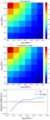 |
Fig. A.1. Normalized sample covariance between mass bins from simulations (top) and our analytical model (center), computed for 106 spherical sub-boxes of radius R = 200 h−1 Mpc at redshift z = 0.506 and in the mass range of 1014 ≤ M/M⊙ ≤ 1016. Bottom panel: relative difference between simulations and model for the diagonal elements of the sample covariance matrix (blue) and for the shot-noise (red). |
In Fig. A.2 we show the (maximum) sample variance contribution relative to the shot-noise level, as a function of the filtering scale, for different redshifts. The curves show that the level of sample variance is lower at high redshift, where the shot-noise dominates due to the small number of objects. Instead, at low redshift (z < 1) the sample variance level is even higher than the shot-noise one, and increase as the radius of the spheres decrease; this means that, at least at low redshift where the volumes of the redshift slices in the light cones are small, such a contribution cannot be neglected, not to introduce systematics or underestimate the error on the parameter constraints.
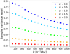 |
Fig. A.2. Sample variance level with respect to the shot-noise, in the lowest mass bin, as a function of the filtering scale R, at different redshifts. |
Appendix B: Application to other surveys
We repeated the likelihood comparison by mimicking other surveys of galaxy clusters, which differ in their volume sampled and their mass and redshift ranges. More specifically, we consider a Planck-like (Tauber et al. 2010) and an SPT-like (Carlstrom et al. 2011) cluster survey, both selected through the Sunyaev–Zeldovich effect, which represent two of the main currently available cluster surveys. We also analyse an eROSITA-like (Predehl 2014) X-ray cluster sample, an upcoming survey that, although not reaching the level of statics that will be provided by Euclid, will produce a much larger sample than current surveys.
The light cones have been extracted from our catalogs, by considering the properties (aperture, selection function, redshift range) of the three surveys, as provided by Bocquet et al. (2016, see Fig. 4 in their paper)5.
The properties of the surveys are as follows:
-
SPT-like sample: we consider light cones with an area of 2500 deg2, containing halos with redshifts z > 0.25 and masses M500c ≥ 3 × 10¹⁴ M⊙. We obtain catalogs with ∼ 1100 objects. We analyze the redshift range 0.25 ≤ z ≤ 1.5 with bins of width Δz = 0.2 and the mass range 3 × 10¹⁴ ≤ M500c/M⊙ ≤ 3 × 10¹⁵, divided in ten bins for the Poissonian case and three bins for the Gaussian case.
-
Planck-like sample: we use the redshift-dependent selection function shown in the reference paper. Since the aperture of the Planck survey is about twice the size of that of Euclid, we stack together two light cones to obtain a Planck-like light-cone; each of the 500 resulting samples contains ∼650 objects. We consider the redshift range of 0 ≤ z ≤ 0.8 with Δz = 0.25 and mass range 1014 ≤ Mvir/M⊙ ≤ 1016; the number of mass bins varies for different redshift bins due to the redshift-dependent selection function, and it is chosen in order to have non-empty bins at each redshift (at least ten objects per bin).
-
eROSITA-like sample: we select halos according to the redshift-dependent selection function given by M500c(z) ≥ 2.3 z × 1014 M⊙, with a mass cut at 7 × 10¹³ M⊙. We analyze the redshift range 0 ≤ z ≤ 2 with Δz = 0.1 and the mass range 1014 ≤ Mvir/M⊙ ≤ 1016 with binning defined in order to have non-empty redshift bins, as for the Planck case. Also in this case, we stack together four PINOCCHIO light cones to create a full-sky eROSITA light-cone, obtaining 250 samples containing ∼2 × 10⁵ objects. For the purpose of this analysis, we did not include any sensitivity mask to account for the different depths of different surveyed area, due to the eROSITA scanning strategy.
In Fig. B.1, we show the distribution of cluster masses of the three samples with their selection function, for comparison to the full Euclid-like catalog. For both SPT and Planck, despite the different selection functions that favour different mass and redshift ranges, the number of objects is low, so we expect shot-noise to be the main source of uncertainty. In contrast, the eROSITA sample contains a larger number of halos, which should lower the level of shot-noise and make the sample variance non-negligible.
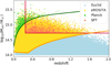 |
Fig. B.1. Mass distribution of the three samples extracted from a single light-cone, with the respective selection functions: Planck in green, SPT in red and eROSITA in orange, overplotted to the full Euclid sample in blue. |
In Fig. B.2, we show the resulting average contours for the Planck and SPT samples, obtained with the Poissonian and Gaussian (full covariance) likelihood functions. In both the cases, the contours from the Gaussian case coincide with the Poissonian ones, confirming that for their survey properties, which produce a low number of objects, the shot-noise dominates over the sample variance. Thus, the use of the Poissonian likelihood still represents a good approximation that does not introduce significant differences at the level of statistics given by the present surveys. Moreover, no systematic effects related to uncertainties in the relation between mass and observable (integrated Compton-y parameter in this case), have been included in the analysis. Unlike Euclid, for these surveys such an uncertainty is expected to dominate the resulting uncertainty on the cosmological parameters (Bocquet et al. 2015), thus making the choice of the likelihood function conservative, since the posteriors would be larger and the effect of theoretical systematics less significant.
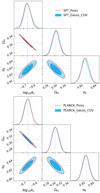 |
Fig. B.2. Contour plots at 68 and 95 per cent of confidence level for the Poissonian (red) and Gaussian (blue) likelihood for the SPT-like (top) and Planck-like (bottom) samples. The gray dotted lines represent the input values of parameters. |
In Fig. B.3, we show the same result for the eROSITA case. We note that there is a large difference between the Poissonian and the Gaussian case, due to the inclusion of the sample variance effect. Such a difference can be ascribed to the mass selection of the survey, which makes the Gaussian contours wider due to the fact that for an X-ray selection, the statistics of counts is dominated by low-redshift-and-low-mass objects distributed within a relatively small volume, which makes the contribution of sample variance becoming comparable to, or dominant over, the shot-noise.
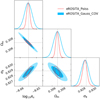 |
Fig. B.3. Contour plots at 68 and 95 per cent of confidence level for the Poissonian (red) and Gaussian (blue) likelihood for the eROSITA-like sample. The gray dotted lines represent the input values of parameters. |
All Figures
|
Fig. 1. Halo mass function for the mass calibration of the PINOCCHIO catalogs. Top panel: comparison between the mass function from the calibrated (red) and the non-calibrated (blue) light cones, averaged over the 1000 catalogs, in the redshift bin z = 0.1 − 0.2. Error bars represent the standard error on the mean. The black line is the D16 mass function. Bottom panel: relative difference between the mass function from simulations and that of D16. |
| In the text | |
|
Fig. 2. Comparison between the T10 halo bias and the bias from the simulations. Top panel: halo bias from simulations at different redshifts (colored dots), compared to the analytical model of T10 (lighter solid lines). Bottom panel: fractional differences between the bias from simulations and from the model. |
| In the text | |
|
Fig. 3. Normalized sample covariance between redshift and mass bins (Eq. (24)), from simulations (left) and analytical model (right). The matrices are computed in the redshift range 0 ≤ z ≤ 1 with Δz = 0.2 and the mass range 1014 ≤ M/M⊙ ≤ 1016, divided into five bins. Black lines denote the redshift bins, while in each black square, there are different mass bins. |
| In the text | |
|
Fig. 4. Covariance (upper panel) and covariance normalized to the shot-noise level (central panel) as predicted by the Hu & Kravtsov (2003) analytical model (solid lines) and by simulations (dashed lines) for different matrix components: diagonal sample variance terms in blue, diagonal sample variance terms in two different mass bins in red and orange, sample variance between two adjacent redshift bins in green and shot-noise in gray. Lower panel: relative difference between analytical model and simulations. The curves are represented as a function of redshift, in the first mass bin (i = 1). |
| In the text | |
|
Fig. 5. Figure of merit for the Poissonian likelihood as a function of the redshift bin widths, for different numbers of mass bins. The points represent the average value over five realizations and the error bars are the standard error of the mean. A small horizontal offset has been applied to make the comparison clearer. |
| In the text | |
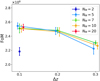 |
Fig. 6. Same as Fig. 5, for the Gaussian likelihood. |
| In the text | |
|
Fig. 7. Contour plots at 68 and 95 per cent of confidence level for the three likelihood functions: Poissonian (red), Gaussian with only shot-noise (orange) and Gaussian with shot-noise and sample variance, with covariance from the analytical model (blue) and from simulations (black). The gray dotted lines represent the input values of parameters. |
| In the text | |
|
Fig. 8. Figure of merit for the different likelihood models: Poissonian, Gaussian with shot-noise, Gaussian with full covariance from simulations, Gaussian with full covariance from the model and Gaussian with block-diagonal covariance from the model. |
| In the text | |
|
Fig. 9. Contour plots at 68 and 95 per cent of confidence level for the Gaussian likelihood with full covariance (blue) and the Gaussian likelihood with block-diagonal covariance (black). The gray dotted lines represent the input values of parameters. |
| In the text | |
|
Fig. 10. Contour plots at the 68 and 95 percent confidence levels for the Gaussian likelihood evaluated with: a cosmology-dependent covariance matrix (black), a covariance matrix fixed at the input cosmology (blue) and covariance matrices computed at two wrong cosmologies, one with lower parameter values (Ωm = 0.295, log10 As = −8.685 and σ8 = 0.776, red) and one with higher parameter values (Ωm = 0.320, log10 As = −8.625 and σ8 = 0.884, orange). The gray dotted lines represent the input values of parameters. |
| In the text | |
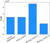 |
Fig. 11. Figure of merit for the models described in Fig. 10. |
| In the text | |
|
Fig. A.1. Normalized sample covariance between mass bins from simulations (top) and our analytical model (center), computed for 106 spherical sub-boxes of radius R = 200 h−1 Mpc at redshift z = 0.506 and in the mass range of 1014 ≤ M/M⊙ ≤ 1016. Bottom panel: relative difference between simulations and model for the diagonal elements of the sample covariance matrix (blue) and for the shot-noise (red). |
| In the text | |
|
Fig. A.2. Sample variance level with respect to the shot-noise, in the lowest mass bin, as a function of the filtering scale R, at different redshifts. |
| In the text | |
|
Fig. B.1. Mass distribution of the three samples extracted from a single light-cone, with the respective selection functions: Planck in green, SPT in red and eROSITA in orange, overplotted to the full Euclid sample in blue. |
| In the text | |
|
Fig. B.2. Contour plots at 68 and 95 per cent of confidence level for the Poissonian (red) and Gaussian (blue) likelihood for the SPT-like (top) and Planck-like (bottom) samples. The gray dotted lines represent the input values of parameters. |
| In the text | |
|
Fig. B.3. Contour plots at 68 and 95 per cent of confidence level for the Poissonian (red) and Gaussian (blue) likelihood for the eROSITA-like sample. The gray dotted lines represent the input values of parameters. |
| In the text | |
Current usage metrics show cumulative count of Article Views (full-text article views including HTML views, PDF and ePub downloads, according to the available data) and Abstracts Views on Vision4Press platform.
Data correspond to usage on the plateform after 2015. The current usage metrics is available 48-96 hours after online publication and is updated daily on week days.
Initial download of the metrics may take a while.