| Issue |
A&A
Volume 683, March 2024
|
|
|---|---|---|
| Article Number | A253 | |
| Number of page(s) | 19 | |
| Section | Cosmology (including clusters of galaxies) | |
| DOI | https://doi.org/10.1051/0004-6361/202245540 | |
| Published online | 22 March 2024 | |
Euclid preparation
XXXV. Covariance model validation for the two-point correlation function of galaxy clusters
1
Dipartimento di Fisica – Sezione di Astronomia, Università di Trieste, Via Tiepolo 11, 34131 Trieste, Italy
e-mail: This email address is being protected from spambots. You need JavaScript enabled to view it.
2
INAF-Osservatorio Astronomico di Trieste, Via G. B. Tiepolo 11, 34143 Trieste, Italy
3
IFPU, Institute for Fundamental Physics of the Universe, Via Beirut 2, 34151 Trieste, Italy
4
INFN, Sezione di Trieste, Via Valerio 2, 34127 Trieste, TS, Italy
5
Laboratoire Univers et Théorie, Observatoire de Paris, Université PSL, Université Paris Cité, CNRS, 92190 Meudon, France
6
Université Paris-Saclay, CNRS, Institut d’Astrophysique Spatiale, 91405 Orsay, France
7
INAF-Osservatorio di Astrofisica e Scienza dello Spazio di Bologna, Via Piero Gobetti 93/3, 40129 Bologna, Italy
8
Dipartimento di Fisica e Astronomia “Augusto Righi” – Alma Mater Studiorum Università di Bologna, Via Piero Gobetti 93/2, 40129 Bologna, Italy
9
INFN-Sezione di Bologna, Viale Berti Pichat 6/2, 40127 Bologna, Italy
10
Max Planck Institute for Extraterrestrial Physics, Giessenbachstr. 1, 85748 Garching, Germany
11
INAF-Osservatorio Astrofisico di Torino, Via Osservatorio 20, 10025 Pino Torinese, TO, Italy
12
Dipartimento di Fisica, Università di Genova, Via Dodecaneso 33, 16146 Genova, Italy
13
INFN-Sezione di Roma Tre, Via della Vasca Navale 84, 00146 Roma, Italy
14
Department of Physics “E. Pancini”, University Federico II, Via Cinthia 6, 80126 Napoli, Italy
15
INAF-Osservatorio Astronomico di Capodimonte, Via Moiariello 16, 80131 Napoli, Italy
16
Instituto de Astrofísica e Ciências do Espaço, Universidade do Porto, CAUP, Rua das Estrelas, 4150-762 Porto, Portugal
17
Dipartimento di Fisica, Università degli Studi di Torino, Via P. Giuria 1, 10125 Torino, Italy
18
INFN-Sezione di Torino, Via P. Giuria 1, 10125 Torino, Italy
19
INAF-IASF Milano, Via Alfonso Corti 12, 20133 Milano, Italy
20
Institut de Física d’Altes Energies (IFAE), The Barcelona Institute of Science and Technology, Campus UAB, 08193 Bellaterra, Barcelona, Spain
21
Port d’Informació Científica, Campus UAB, C. Albareda s/n, 08193 Bellaterra, Barcelona, Spain
22
Institut d’Estudis Espacials de Catalunya (IEEC), Carrer Gran Capitá 2-4, 08034 Barcelona, Spain
23
Institute of Space Sciences (ICE, CSIC), Campus UAB, Carrer de Can Magrans, s/n, 08193 Barcelona, Spain
24
INAF-Osservatorio Astronomico di Roma, Via Frascati 33, 00078 Monteporzio Catone, Italy
25
INFN Section of Naples, Via Cinthia 6, 80126 Napoli, Italy
26
Centre National d’Études Spatiales – Centre Spatial de Toulouse, 18 Avenue Édouard Belin, 31401 Toulouse Cedex 9, France
27
Institut National de Physique Nucléaire et de Physique des Particules, 3 Rue Michel-Ange, 75794 Paris Cédex 16, France
28
Institute for Astronomy, University of Edinburgh, Royal Observatory, Blackford Hill, Edinburgh EH9 3HJ, UK
29
Jodrell Bank Centre for Astrophysics, Department of Physics and Astronomy, University of Manchester, Oxford Road, Manchester M13 9PL, UK
30
ESAC/ESA, Camino Bajo del Castillo, s/n., Urb. Villafranca del Castillo, 28692 Villanueva de la Cañada, Madrid, Spain
31
European Space Agency/ESRIN, Largo Galileo Galilei 1, 00044 Frascati, Roma, Italy
32
University of Lyon, Univ. Claude Bernard Lyon 1, CNRS/IN2P3, IP2I Lyon, UMR 5822, 69622 Villeurbanne, France
33
Institute of Physics, Laboratory of Astrophysics, Ecole Polytechnique Fédérale de Lausanne (EPFL), Observatoire de Sauverny, 1290 Versoix, Switzerland
34
Mullard Space Science Laboratory, University College London, Holmbury St Mary, Dorking, Surrey RH5 6NT, UK
35
Departamento de Física, Faculdade de Ciências, Universidade de Lisboa, Edifício C8, Campo Grande, 1749-016 Lisboa, Portugal
36
Instituto de Astrofísica e Ciências do Espaço, Faculdade de Ciências, Universidade de Lisboa, Campo Grande, 1749-016 Lisboa, Portugal
37
Department of Astronomy, University of Geneva, Ch. d’Ecogia 16, 1290 Versoix, Switzerland
38
INFN-Padova, Via Marzolo 8, 35131 Padova, Italy
39
Université Paris-Saclay, Université Paris Cité, CEA, CNRS, Astrophysique, Instrumentation et Modélisation Paris-Saclay, 91191 Gif-sur-Yvette, France
40
Aix-Marseille Université, CNRS/IN2P3, CPPM, 13288 Marseille, France
41
Istituto Nazionale di Fisica Nucleare, Sezione di Bologna, Via Irnerio 46, 40126 Bologna, Italy
42
INAF-Osservatorio Astronomico di Padova, Via dell’Osservatorio 5, 35122 Padova, Italy
43
Universitäts-Sternwarte München, Fakultät für Physik, Ludwig-Maximilians-Universität München, Scheinerstrasse 1, 81679 München, Germany
44
Institute of Theoretical Astrophysics, University of Oslo, PO Box 1029 Blindern 0315 Oslo, Norway
45
Jet Propulsion Laboratory, California Institute of Technology, 4800 Oak Grove Drive, Pasadena, CA 91109, USA
46
Technical University of Denmark, Elektrovej 327, 2800 Kgs. Lyngby, Denmark
47
Cosmic Dawn Center (DAWN), Copenhagen, Denmark
48
Institut d’Astrophysique de Paris, 98bis Boulevard Arago, 75014 Paris, France
49
Max-Planck-Institut für Astronomie, Königstuhl 17, 69117 Heidelberg, Germany
50
Université de Genève, Département de Physique Théorique and Centre for Astroparticle Physics, 24 quai Ernest-Ansermet, 1211 Genève 4, Switzerland
51
Department of Physics, University of Helsinki, PO Box 64 00014 Helsinki, Finland
52
Helsinki Institute of Physics, University of Helsinki, Gustaf Hällströmin katu 2, Helsinki, Finland
53
NOVA Optical Infrared Instrumentation Group at ASTRON, Oude Hoogeveensedijk 4, 7991 PD Dwingeloo, The Netherlands
54
Argelander-Institut für Astronomie, Universität Bonn, Auf dem Hügel 71, 53121 Bonn, Germany
55
Department of Physics, Institute for Computational Cosmology, Durham University, South Road, DH1 3LE Durham, UK
56
Université Côte d’Azur, Observatoire de la Côte d’Azur, CNRS, Laboratoire Lagrange, Bd de l’Observatoire, CS 34229, 06304 Nice Cedex 4, France
57
Université Paris Cité, CNRS, Astroparticule et Cosmologie, 75013 Paris, France
58
European Space Agency/ESTEC, Keplerlaan 1, 2201 AZ Noordwijk, The Netherlands
59
Department of Physics and Astronomy, University of Aarhus, Ny Munkegade 120, 8000 Aarhus C, Denmark
60
Centre for Astrophysics, University of Waterloo, Waterloo, Ontario N2L 3G1, Canada
61
Department of Physics and Astronomy, University of Waterloo, Waterloo, Ontario N2L 3G1, Canada
62
Perimeter Institute for Theoretical Physics, Waterloo, Ontario N2L 2Y5, Canada
63
AIM, CEA, CNRS, Université Paris-Saclay, Université de Paris, 91191 Gif-sur-Yvette, France
64
Space Science Data Center, Italian Space Agency, Via del Politecnico snc, 00133 Roma, Italy
65
Instituto de Astrofísica de Canarias, Calle Vía Láctea s/n, 38204 San Cristóbal de La Laguna, Tenerife, Spain
66
Departamento de Astrofísica, Universidad de La Laguna, 38206 La Laguna, Tenerife, Spain
67
Dipartimento di Fisica e Astronomia “G. Galilei”, Università di Padova, Via Marzolo 8, 35131 Padova, Italy
68
Departamento de Física, FCFM, Universidad de Chile, Blanco Encalada, 2008 Santiago, Chile
69
Centro de Investigaciones Energéticas, Medioambientales y Tecnológicas (CIEMAT), Avenida Complutense 40, 28040 Madrid, Spain
70
Instituto de Astrofísica e Ciências do Espaço, Faculdade de Ciências, Universidade de Lisboa, Tapada da Ajuda, 1349-018 Lisboa, Portugal
71
Universidad Politécnica de Cartagena, Departamento de Electrónica y Tecnología de Computadoras, Plaza del Hospital 1, 30202 Cartagena, Spain
72
Institut de Recherche en Astrophysique et Planétologie (IRAP), Université de Toulouse, CNRS, UPS, CNES, 14 Av. Édouard Belin, 31400 Toulouse, France
73
Infrared Processing and Analysis Center, California Institute of Technology, Pasadena, CA 91125, USA
74
INAF-Osservatorio Astronomico di Brera, Via Brera 28, 20122 Milano, Italy
75
Center for Computational Astrophysics, Flatiron Institute, 162 5th Avenue, 10010 New York, NY, USA
76
School of Physics and Astronomy, Cardiff University, The Parade, Cardiff CF24 3AA, UK
77
INAF-Istituto di Astrofisica e Planetologia Spaziali, Via del Fosso del Cavaliere, 100, 00100 Roma, Italy
78
Dipartimento di Fisica “Aldo Pontremoli”, Università degli Studi di Milano, Via Celoria 16, 20133 Milano, Italy
79
INFN-Sezione di Milano, Via Celoria 16, 20133 Milano, Italy
80
Dipartimento di Fisica e Astronomia “Augusto Righi” – Alma Mater Studiorum Università di Bologna, Viale Berti Pichat 6/2, 40127 Bologna, Italy
81
Junia, EPA Department, 41 Bd Vauban, 59800 Lille, France
82
SISSA, International School for Advanced Studies, Via Bonomea 265, 34136 Trieste, TS, Italy
83
Dipartimento di Fisica e Scienze della Terra, Università degli Studi di Ferrara, Via Giuseppe Saragat 1, 44122 Ferrara, Italy
84
Istituto Nazionale di Fisica Nucleare, Sezione di Ferrara, Via Giuseppe Saragat 1, 44122 Ferrara, Italy
85
Institut d’Astrophysique de Paris, UMR 7095, CNRS, and Sorbonne Université, 98 bis Boulevard Arago, 75014 Paris, France
86
Institut de Physique Théorique, CEA, CNRS, Université Paris-Saclay, 91191 Gif-sur-Yvette Cedex, France
87
NASA Ames Research Center, Moffett Field, CA 94035, USA
88
INAF, Istituto di Radioastronomia, Via Piero Gobetti 101, 40129 Bologna, Italy
89
INFN-Bologna, Via Irnerio 46, 40126 Bologna, Italy
90
Institute for Theoretical Particle Physics and Cosmology (TTK), RWTH Aachen University, 52056 Aachen, Germany
91
Institute for Astronomy, University of Hawaii, 2680 Woodlawn Drive, Honolulu, HI 96822, USA
92
Department of Physics & Astronomy, University of California Irvine, Irvine, CA 92697, USA
93
University of Lyon, UCB Lyon 1, CNRS/IN2P3, IUF, IP2I Lyon, 4 Rue Enrico Fermi, 69622 Villeurbanne, France
94
INFN-Sezione di Genova, Via Dodecaneso 33, 16146 Genova, Italy
95
Aix-Marseille Université, CNRS, CNES, LAM, 13388 Marseille, France
96
Department of Astronomy & Physics and Institute for Computational Astrophysics, Saint Mary’s University, 923 Robie Street, Halifax, Nova Scotia B3H 3C3, Canada
97
Department of Physics, Oxford University, Keble Road, Oxford OX1 3RH, UK
98
Instituto de Física Teórica UAM-CSIC, Campus de Cantoblanco, 28049 Madrid, Spain
99
University Observatory, Faculty of Physics, Ludwig-Maximilians-Universität, Scheinerstr. 1, 81679 Munich, Germany
100
Ruhr University Bochum, Faculty of Physics and Astronomy, Astronomical Institute (AIRUB), German Centre for Cosmological Lensing (GCCL), 44780 Bochum, Germany
101
Department of Physics, Lancaster University, Lancaster LA1 4YB, UK
102
Univ. Grenoble Alpes, CNRS, Grenoble INP, LPSC-IN2P3, 53 Avenue des Martyrs, 38000 Grenoble, France
103
Department of Physics and Astronomy, University College London, Gower Street, London WC1E 6BT, UK
104
Department of Physics and Helsinki Institute of Physics, University of Helsinki, Gustaf Hällströmin katu 2, 00014 Helsinki, Finland
105
Astrophysics Group, Blackett Laboratory, Imperial College London, London SW7 2AZ, UK
106
Dipartimento di Fisica, Sapienza Università di Roma, Piazzale Aldo Moro 2, 00185 Roma, Italy
107
University of Applied Sciences and Arts of Northwestern Switzerland, School of Engineering, 5210 Windisch, Switzerland
108
Institut für Theoretische Physik, University of Heidelberg, Philosophenweg 16, 69120 Heidelberg, Germany
109
Zentrum für Astronomie, Universität Heidelberg, Philosophenweg 12, 69120 Heidelberg, Germany
110
Institute of Cosmology and Gravitation, University of Portsmouth, Portsmouth PO1 3FX, UK
111
Department of Mathematics and Physics E. De Giorgi, University of Salento, Via per Arnesano, CP-I93, 73100 Lecce, Italy
112
INAF-Sezione di Lecce, c/o Dipartimento Matematica e Fisica, Via per Arnesano, 73100 Lecce, Italy
113
INFN, Sezione di Lecce, Via per Arnesano, CP-193, 73100 Lecce, Italy
114
Institute of Space Science, Str. Atomistilor, nr. 409 Măgurele, Ilfov 077125, Romania
115
Institute for Computational Science, University of Zurich, Winterthurerstrasse 190, 8057 Zurich, Switzerland
116
Higgs Centre for Theoretical Physics, School of Physics and Astronomy, The University of Edinburgh, Edinburgh EH9 3FD, UK
117
Université St Joseph; Faculty of Sciences, Beirut, Lebanon
Received:
23
November
2022
Accepted:
5
December
2023
Abstract
Aims. We validate a semi-analytical model for the covariance of the real-space two-point correlation function of galaxy clusters.
Methods. Using 1000 PINOCCHIO light cones mimicking the expected Euclid sample of galaxy clusters, we calibrated a simple model to accurately describe the clustering covariance. Then, we used this model to quantify the likelihood-analysis response to variations in the covariance, and we investigated the impact of a cosmology-dependent matrix at the level of statistics expected for the Euclid survey of galaxy clusters.
Results. We find that a Gaussian model with Poissonian shot-noise does not correctly predict the covariance of the two-point correlation function of galaxy clusters. By introducing a few additional parameters fitted from simulations, the proposed model reproduces the numerical covariance with an accuracy of 10%, with differences of about 5% on the figure of merit of the cosmological parameters Ωm and σ8. We also find that the covariance contains additional valuable information that is not present in the mean value, and the constraining power of cluster clustering can improve significantly when its cosmology dependence is accounted for. Finally, we find that the cosmological figure of merit can be further improved when mass binning is taken into account. Our results have significant implications for the derivation of cosmological constraints from the two-point clustering statistics of the Euclid survey of galaxy clusters.
Key words: methods: statistical / galaxies: clusters: general / cosmological parameters / large-scale structure of Universe
© The Authors 2024
 Open Access article, published by EDP Sciences, under the terms of the Creative Commons Attribution License (https://creativecommons.org/licenses/by/4.0), which permits unrestricted use, distribution, and reproduction in any medium, provided the original work is properly cited.
This article is published in open access under the Subscribe to Open model. This email address is being protected from spambots. You need JavaScript enabled to view it. to support open access publication.
1. Introduction
The clustering of galaxy clusters is an increasingly powerful tool for extracting cosmological information because it is sensitive to the geometry and to the evolution of the large-scale structure of the Universe (Borgani et al. 1999; Moscardini et al. 2000; Estrada et al. 2009; Marulli et al. 2018, 2021). Cluster clustering is still poorly constraining when considered alone because of the small statistics. It is especially useful, however, when it is combined with other probes, such as number counts or weak gravitational lensing, for two main reasons. First, its cosmology dependence is different, which enables breaking the degeneracies on parameters and improving the constraining power of these observables (Schuecker et al. 2003; Sereno et al. 2015; Sartoris et al. 2016). Second, one of the main limitations in the cosmological exploitation of galaxy clusters lies in the fact that cluster masses have to be inferred indirectly through observable properties, such as the cluster richness, the velocity dispersion, the X-ray temperature, or Sunyaev–Zeldovich signal. The calibration of such mass-observable scaling relations is affected by systematic biases and observational uncertainties (e.g. Kravtsov & Borgani 2012; Pratt et al. 2019). Cluster clustering presents different degeneracies on parameters than cluster number counts. It can therefore help to calibrate these relations and reduce the uncertainties in the mass estimation. It can furthermore improve the constraints on cosmological parameters (Majumdar & Mohr 2004; Mana et al. 2013; To et al. 2021a; Lesci et al. 2022). The correlation function of galaxy clusters has also been used to identify baryonic acoustic oscillations (BAOs) independently of the cosmic microwave background (CMB, Miller et al. 2001; Angulo et al. 2005; Huetsi 2010; Veropalumbo et al. 2014; Moresco et al. 2021).
The clustering of clusters presents some advantages with respect to the clustering of galaxies. Rising from the highest density peaks of the density field, galaxy clusters are a highly biased tracer of the large-scale structure, that is, the stronger clustering signal is easily detectable at large scales as well. Cluster clustering can be observed on large scales, where linear theory is still suitable for describing its properties (i.e., k ≲ 0.05 h−1 Mpc or r ≳ 30 h−1 Mpc). Moreover, bias is primarily a function of the halo mass and can be calibrated using multiwavelength observations. Moreover, cosmology enters the relation between bias and mass and redshift and increases the constraining power of cluster clustering (Mo & White 1996; Tinker et al. 2010). Finally, Castro et al. (2020) showed that the net effect of baryons is to change the mass of clusters with negligible impact on the clustering of matched objects in dark matter and hydro simulations. Thus, we can identify the clustering of clusters as the clustering of dark matter halos. For this reason, the terms “cluster” and “halo” are used as synonyms.
The clustering of clusters is expected to become an important source of information within a few years, when upcoming and future surveys will provide cluster samples over sizable portions of the sky. They include the European Space Agency (ESA) mission Euclid1, planned for 2023, which will map ∼15 000 deg2 of the extragalactic sky in optical and near-infrared bands, with the aim of investigating the nature of dark energy, dark matter, and gravity (Laureijs et al. 2011; Euclid Collaboration 2022). Galaxy clusters are one of the cosmological probes to be used by Euclid, for which the mission is expected to yield a sample of ∼105 clusters up to redshift z ∼ 2. Sartoris et al. (2016) showed that the constraints on cosmological parameters from cluster number counts are significantly improved when the cluster clustering information is included in the analysis of a Euclid-like survey.
A fundamental ingredient in deriving precise and accurate constraints on cosmological parameters from these catalogs is the correct description of the uncertainties affecting the observables. The uncertainties are given in the form of covariance matrices. The simplest but a computationally expensive way to compute a covariance matrix is from measurements in a large set of simulations. The computational cost can be reduced by generating mocks with approximate methods instead of full N-body simulations (Monaco 2016) or with mixed methods, such as the shrinkage technique (Pope & Szapudi 2008). However, the resulting matrix will still be noisy unless a large number of mock realizations are generated. If the covariance is considered to be cosmology dependent, the cost will inevitably increase as many more simulations are required to explore the high-dimensional space of cosmological parameters with these simulations. An alternative approach is to estimate covariances from the data themselves by means of bootstrap or jackknife techniques: These methods have the advantage of providing matrices that are evaluated at the true cosmology of the Universe, but the resampling methods tend to overestimate the true covariance, especially for two-point statistics (Norberg et al. 2009; Friedrich et al. 2016; Lacasa & Kunz 2017; Mohammad & Percival 2022). A third method consists of the analytic calculation of the covariance matrix (e.g. Feldman et al. 1994; Scoccimarro et al. 1999; Meiksin & White 1999; Hu & Kravtsov 2003; Takada & Hu 2013), which provides noise-free, cosmology-dependent matrices without requiring expensive computational resources. The limitation of this method lies in the difficulty of analytically describing all the contributions to the covariance (e.g. nonlinearities and non-Gaussianities). Moreover, it is straightforward to include a treatment of systematic errors by imposing a realistic selection function to mock catalogs, while in the case of an analytical model, this is more challenging and likely to require significant approximations. Therefore, these models have to be validated against simulations to determine which contributions are relevant at the required level of statistics. Moreover, in some cases, this validation process may indicate that an analytical description is not sufficient to correctly describe the covariance matrix, and it is thus necessary to calibrate model parameters that cannot be determined from first principles (Xu et al. 2012; O’Connell et al. 2016; Fumagalli et al. 2022).
The covariance of two-point correlation functions is nontrivial to model because it depends on high-order statistics and on the survey geometry (Bernstein 1994; Li et al. 2019). Several works have developed models for the covariance of galaxy correlation functions, both in configuration and Fourier space (see, for instance, Scoccimarro et al. 1999; Meiksin & White 1999; Takada & Hu 2013; Wadekar & Scoccimarro 2020; Philcox & Eisenstein 2019; Li et al. 2019). Galaxy clustering is characterized by a Gaussian covariance, representing the main contribution at large scales, plus a non-Gaussian term arising from nonlinear gravitational instability, galaxy/halo bias, and redshift-space distortions. This term dominates at small scales. In addition, the coupling between short-wavelength modes with perturbations larger than the survey size, also induced by non-Gaussianities, namely supersample covariance, contributes to the error budget on small scales. Last, the shape of the observed volume can also affect the covariance, requiring a convolution of the power spectrum with the window function of the survey. For cluster clustering, the situation is simpler in principle because the scales involved are larger and mostly linear. This feature means that highly nonlinear effects, such as super-sample covariance, can be excluded because it dominates the non-Gaussian errors in the weakly or deeply nonlinear regime (Takada & Hu 2013). However, the lower densities characterizing these objects produce a different weight of the various contributions (e.g. shot noise, Paech et al. 2017) to the covariance, compared to the case of galaxies, which could make non-Gaussian terms relevant even in the linear regime. Up to now, the analytical covariance for cluster clustering has rarely been studied (Valageas et al. 2011; To et al. 2021b), and numerical methods or internal estimates were preferred instead.
This work represents a second paper in a series, following Euclid Collaboration (2021). We validate a semi-analytical model for the covariance of the two-point correlation function (2PCF hereafter) of clusters by comparison with a numerical matrix. Because the final purpose is to apply this model covariance in the analysis of photometric data, we simply consider the real-space clustering. The redshift-space distortions of the monopole of the 2PCF are negligible with respect to the distortion produced by the photo-z uncertainties (Veropalumbo et al. 2014; Sereno et al. 2015; Lesci et al. 2022). We test the validity of a Gaussian model, with the addition of a low-order non-Gaussian term. We are interested in understanding whether this simple model is suitable to describe the covariance for the future survey of galaxy clusters to be extracted from the Euclid photometric survey by estimating the impact of the missing high-order terms and of the shot noise. Then, we focus our attention on the study of the cosmology dependence of the covariance to determine whether this dependence can help us obtain a more precise estimate of the cosmological parameters. Last, we test the impact of mass binning on the cosmological constraints. We perform the validation of the covariance for a Vanilla ΛCDM cosmological model by studying the effect of the covariance on the cosmological constraints of the parameters Ωm and σ8.
The paper is structured as follows: In Sect. 2 we introduce the analytical formalism for describing the 2PCF and its covariance, as well as the formalism for the likelihood analysis and the estimation of the posteriors accuracy. In Sect. 3 we describe the simulated data: in Sect. 3.1 we present the simulations we used to measure the numerical matrix and the cosmological forecasts, and in Sect. 3.2 we describe the measurements of the 2PCF and the associated numerical covariance. In Sect. 4 we present the results of our analysis: In Sect. 4.1 we define the best binning in spatial separation and redshift to extract the cosmological information, and in Sect. 4.2 we compare the analytical and numerical matrices. We introduce additional parameters to improve the agreement between the two covariances. Further motivations for introducing these additional parameters are discussed in Appendix B, and the result of the fit of these parameters is detailed presented in Appendix C. In Sect. 4.3 we study the impact of the non-Gaussian term, and in Sect. 4.4 we investigate the effect of the cosmology-dependent matrix. More considerations about the cosmology-dependence are presented in Appendices D and E. In Sect. 4.5 we evaluate the impact of the mass binning. Finally, in Sect. 5 we discuss our conclusions.
2. Theoretical background
In this section, we introduce the real-space 2PCF of halos and its covariance matrix model. We also describe the likelihood we adopted for the parameter inference and the method for assessing the accuracy of the results.
2.1. Two-point correlation function
We quantified the clustering of clusters with the real-space 2PCF, describing the excess number of pairs with respect to a random distribution, as a function of radial separation and redshift. This function is defined as the Fourier transform of the halo power spectrum,
 (1)
(1)
where Pm(k, z) is the matter power spectrum, j0(kr) is the zero-order spherical Bessel function, r is the comoving radial separation, and  is the effective linear bias, that is, the linear halo bias integrated above the mass threshold M,
 (2)
(2)
where dn/dM is the halo mass function, and  is the mean number density of objects above a mass threshold
 (3)
(3)
In the following, we adopt the Despali et al. (2016) model to describe the halo mass function (Eq. (7) in the paper) and the Tinker et al. (2010) model for the halo bias (Eq. (6) in the paper).
For the sake of simplicity, we validated our model considering halos with a mass above a fixed threshold; subsequently, in Sect. 2.3, we extend the discussion to the case with mass binning.
Although we worked in linear theory, around the BAO scale rBAO ≃ 110 h−1 Mpc (Eisenstein et al. 2005; Cole et al. 2005) we account for the smoothing of the acoustic features induced by a large-scale coherent flow. This produces a broadening and a shift of the BAO peak in the 2PCF (Eisenstein et al. 2007), which can be modeled by the infrared resummation (Senatore & Zaldarriaga 2015; Baldauf et al. 2015). At the lowest order, the matter power spectrum is corrected as
 (4)
(4)
where Pw and Pnw are the wiggle and smooth parts of the linear power spectrum, respectively, and
![Mathematical equation: $$ \begin{aligned} \Sigma ^2(z) = \int _0^{k_s}\frac{{\mathrm{d}} q}{6\pi ^2}\, P_{\rm nw}(q,z)\,\left[1-j_0\left(q\,r_{\rm BAO}\right)+2j_2\left(q\,r_{\rm BAO}\right)\right]. \end{aligned} $$](/articles/aa/full_html/2024/03/aa45540-22/aa45540-22-eq7.gif) (5)
(5)
The final expression for the real-space 2PCF of halos to be compared with observations is obtained by averaging Eq. (1) over the ath redshift bin and ith separation bin,
 (6)
(6)
where ⟨ ⟩a indicates the average over the redshift bin,
 (7)
(7)
where dV/dz = Ωsky dV/dΩ dz is the comoving volume per unit redshift, and Ωsky is the survey area in steradians2. Wi(k) represents the spherical shell window function, given by
 (8)
(8)
where Wth(kr) is the top-hat window function, Vi is the volume of the ith spherical shell, and ri, −, ri, + are the extremes of the separation bin.
2.2. Covariance model
The 2PCF covariance can be obtained as the Fourier transform of the power spectrum covariance. The latter is defined as
![Mathematical equation: $$ \begin{aligned} C_P(\mathbf k _1, \mathbf k _2) = \left\langle \left[\hat{P}_{\rm h}(\mathbf k _1) - \langle \hat{P}_{\rm h}(\mathbf k _1) \rangle \right] \, \left[ \hat{P}_{\rm h}(\mathbf k _2) - \langle \hat{P}_{\rm h}(\mathbf k _2) \rangle \right] \right\rangle , \end{aligned} $$](/articles/aa/full_html/2024/03/aa45540-22/aa45540-22-eq11.gif) (9)
(9)
where
 (10)
(10)
is the estimator for the halo power spectrum, such that  . Here, V is the observed volume and
  is the (Poissonian) shot-noise correction for the halo power spectrum Ph.
Substituting the power spectrum estimator in Eq. (9), we obtain the expression of the power spectrum covariance (Meiksin & White 1999; Scoccimarro et al. 1999)
![Mathematical equation: $$ \begin{aligned} \begin{aligned} C_P(\mathbf k _1, \mathbf k _2) =& \frac{(2 \pi )^3}{V} \left[ P_{\rm h}(k) + \frac{1}{{\overline{n}}} \right]^2 \left[ \delta ^\mathrm{K}(\mathbf k _1-\mathbf k _2) + \delta ^\mathrm{K}(\mathbf k _1+\mathbf k _2)\right] \\& + \frac{1}{V\,{\overline{n}}^2}\, \bigg [ P_{\rm h}(|\mathbf k _1-\mathbf k _2|) + P_{\rm h}(|\mathbf k _1+\mathbf k _2|) + 2P_{\rm h}(k) + 2P_{\rm h}(k_2) \bigg ] \\& + \frac{1}{V\,{\overline{n}}} \, \bigg [ B_{\rm h}(\mathbf k _1,-\mathbf k _1,0) + B_{\rm h}(\mathbf k _2,-\mathbf k _2,0)+ B_{\rm h}(\mathbf k _1,\mathbf k _2)\\& + B_{\rm h}(\mathbf k _1,-\mathbf k _2) + B_{\rm h}(-\mathbf k _1,\mathbf k _2) + B_{\rm h}(-\mathbf k _1, -\mathbf k _2) \bigg ] \\& + \frac{1}{V} \, {T_{\rm h}(\mathbf k _1,\mathbf -k ,\mathbf k _2,\mathbf -k_2 )} + \frac{1}{V \, {\overline{n}}^3}, \end{aligned} \end{aligned} $$](/articles/aa/full_html/2024/03/aa45540-22/aa45540-22-eq15.gif) (11)
(11)
where Bh and Th are the bispectrum and the trispectrum of halos, respectively, that is, the three- and four-point correlation functions in Fourier space. The first line represents the Gaussian covariance, and the other lines represent the non-Gaussian component. As explained in Sect. 1, we did not consider the supersample covariance.
By Fourier transforming Eq. (11) and integrating over separation and redshift bins (Cohn 2006), we obtain a model for the 2PCF covariance in the light cone,
![Mathematical equation: $$ \begin{aligned} \begin{aligned} C_{a i j} =&\frac{2}{V_a} \int \frac{{\mathrm{d}} k\,k^2}{2 \pi ^2} \left[ \left\langle {\overline{b}\,}^2P_{\rm m}(k) \right\rangle _a + \left\langle \frac{1}{{\overline{n}}}\right\rangle _a \right]^2 W_i(k) \, W_j(k)\\&+ \frac{2}{V_a V_i} \int \frac{{\mathrm{d}} k\,k^2}{2 \pi ^2} \left\langle {\overline{b}\,}^2 P_{\rm m}(k)\right\rangle _a \left\langle \frac{1}{{\overline{n}}}\right\rangle ^2_a \, W_j(k) \ \delta _{ij}, \end{aligned} \end{aligned} $$](/articles/aa/full_html/2024/03/aa45540-22/aa45540-22-eq16.gif) (12)
(12)
where i, j states for the two separation bins, while the a index is for the average over the redshift bin, and Va is the volume of the redshift slice. The model in Eq. (12) clearly is a simplification of the full covariance matrix based on the following approximations:
-
By considering large redshift slices (Δz ≳ 0.2), we assumed that the cross-correlation between redshift bins is negligible, as verified from the numerical matrix, computed with Eq. (22). The comparison is shown in Fig. 4 (upper versus lower triangle).
-
We neglect the contribution from higher-order correlation functions and only include the lowest-order shot-noise contributions of the non-Gaussian covariance in addition to the Gaussian part.
-
We do not include the terms that only contribute at zero separation (∝δD(ri),δD(rj)) because we consider larger scales.
-
We do not account for the survey footprint, but consider a simplistic window function described by a fixed-size opening angle.
2.3. Mass binning
We now extend the formalism to take the mass binning instead of a simple mass threshold into account to quantify the amount of information that is contained in the mass dependence of the halo bias.
We rewrote Eq. (1) as
 (13)
(13)
and all the equations derived in Sect. 2 were modified according to this change. We obtained the binned 2PCF by integrating Eq. (13) over the ith separation bin, the ath redshift bin, and between Ath and Bth mass bins. The integrals over mass (Eqs. (2) and (3)) were now performed between the edges of each mass bin. The final binned 2PCF takes both the autocorrelation inside a single mass interval and the cross-correlation between halos belonging to two different mass bins into account,
 (14)
(14)
Consequently, the covariance matrix was adapted to account for four terms: for the autocorrelation between auto-2PCFs (CAAAA), for the autocorrelation between cross-2PCFs (CABAB), for the crosscorrelation between auto-2PCFs (CAABB), and for the cross correlation between cross-2PCFs (CABCD). The covariance model between different mass bins can be treated as the covariance between multiprobes (Smith 2009; Hu & Jain 2004; Krause & Eifler 2017), that is,
 (15)
(15)
Following the demonstration reported in Appendix A, the cross covariance between different mass, redshift, and radial bins is given by
![Mathematical equation: $$ \begin{aligned} \begin{aligned} C_{aij}^{ABCD} =& \frac{1}{V_a} \int \frac{{\mathrm{d}} k\,k^2}{2 \pi ^2} \left[ \left\langle \,{\overline{b}}_A\,{\overline{b}}_C\,P_{\rm m}(k) \right\rangle _a + \left\langle \frac{\delta _{AC}}{{\overline{n}_A}} \right\rangle _a \right]\\&\times \left[ \left\langle \,{\overline{b}}_B\,{\overline{b}}_D\,P_{\rm m}(k) \right\rangle _a + \left\langle \frac{\delta _{BD}}{{\overline{n}_B}} \, \right\rangle _a \right] \,W_i\,W_j\\&+ \frac{1}{V_a} \int \frac{{\mathrm{d}} k\,k^2}{2 \pi ^2} \left\langle \,{\overline{b}}_A\,{\overline{b}}_B\, P_{\rm m}(k)\right\rangle _a \left\langle \frac{\delta _{AC}}{{\overline{n}_A}}\,\right\rangle _a\,\left\langle \frac{\delta _{BD}}{{\overline{n}_B}}\,\right\rangle _a\frac{W_j}{V_i} \delta _{ij}\\&+ (C \longleftrightarrow D). \end{aligned} \end{aligned} $$](/articles/aa/full_html/2024/03/aa45540-22/aa45540-22-eq20.gif) (16)
(16)
2.4. Likelihood function
We studied the effect of the covariance on cosmological constraints by performing a Bayesian inference on mock cluster surveys extracted from simulations. We explored the posterior distribution with a Monte Carlo Markov chain (MCMC) approach by using a python wrapper for the nested sampling PyMultiNest (Buchner et al. 2014).
We adopted a Gaussian likelihood,
![Mathematical equation: $$ \begin{aligned} \mathcal{L} (\boldsymbol{d} \,\vert \,\boldsymbol{m}(\boldsymbol{\theta }),\,C) = \frac{\exp {\left\{ -\frac{1}{2} [\boldsymbol{d} - \boldsymbol{m}(\boldsymbol{\theta })]^T C^{-1} [\boldsymbol{d} - \boldsymbol{m}(\boldsymbol{\theta })] \right\} }}{\sqrt{(2\pi )^N \vert C \vert }}, \end{aligned} $$](/articles/aa/full_html/2024/03/aa45540-22/aa45540-22-eq21.gif) (17)
(17)
where d is the data vector, m(θ) is the prediction as a function of a set of cosmological parameters θ, and C is the covariance matrix, which may also depend on cosmological parameters.
Unless otherwise specified, we inferred the cosmological parameters by maximizing the log-likelihood function averaged over all the NS simulated catalogs used in this work to remove the effect of cosmic variance that affects the single realization of the Universe,
 (18)
(18)
With this step, we were able to individuate possible systematic effects in the analysis that could introduce small but sizable shifts in the cosmological posteriors with respect to the input parameter values.
We quantified the accuracy of our covariance (error) estimates in terms of the effect on the figure of merit (FoM, Albrecht et al. 2006) for two parameters θ1 and θ2, defined as
 (19)
(19)
where C(θ1, θ2) is the parameter covariance computed from the sampled posteriors. The FoM is proportional to the inverse of the area enclosed by the ellipse representing the 68% confidence level. In general, a higher FoM therefore indicates a more precise evaluation of the parameters. For the covariance comparison, however, a larger FoM could indicate an underestimation of the posteriors amplitude, resulting from an incorrect estimation of the uncertainties on the statistical quantities entering the likelihood. We therefore point out that we are not interested in the absolute value of the FoM, but rather in the difference between the various cases.
3. Simulated data
We describe in this section the simulations we used and the procedure with which we measured the 2PCF and its numerical covariance.
3.1. Simulations
Following Euclid Collaboration (2021), we validated our model by comparing it with a reference covariance, computed numerically from simulations. The use of a large set of simulations is a fundamental requirement for the accurate estimation of covariance matrices. The dimension of this set depends on the size of the data vector (i.e., the total number of bins) and the desired accuracy. Typically, the required number of catalogs is about 103 or even more (Taylor et al. 2013; Dodelson & Schneider 2013). For this purpose, catalogs generated with N-body simulations can hardly be obtained because the computational cost is too high. Instead, large sets of mock data can be produced in a simpler and faster way by using approximate methods based on perturbative theories. Although less accurate than full N-body simulations in reproducing the observables, these methods are able to accurately estimate covariances and require fewer resources and far less computational time (Sahni & Coles 1995; Monaco 2016; Lippich et al. 2019; Blot et al. 2019; Colavincenzo et al. 2019).
We used a set of mock catalogs produced with the PINOCCHIO (PINpointing Orbit-Crossing Collapsed HIerarchical Objects, Monaco et al. 2002; Munari et al. 2017) algorithm. PINOCCHIO generates dark matter halo catalogs using Lagrangian perturbation theory (LPT, Moutarde et al. 1991; Buchert 1992; Bouchet et al. 1995) up to third order and the ellipsoidal collapse (Bond & Myers 1996; Eisenstein & Loeb 1995). The code generates an initial density field on a regular grid with periodic boundary conditions and computes the collapse time of each particle. Then, by means of LPT, it displaces particles to form halos, which are finally moved to their final positions by again applying LPT. In this way, the code is able to simulate large cubic boxes that are used to build the past-light cones. The latter are generated by replicating the periodic boxes through an on-the-fly process, in which only the halos are selected that are causally connected with an observer at the present time.
Our data set consisted of 1000 past-light cones3 each covering an area of 10 313 deg2 and redshift range z = 0 − 2.5.4 The light cones contain halos with virial masses above 3.61 × 10¹³ M⊙, sampled with more than 50 particles. The cosmology used in the simulations is the flat ΛCDM cosmology with parameters fixed according to Planck Collaboration XVI (2014) (Table 5, “Planck+WP+highL+BAO” case): Ωm = 0.30711 for the total matter density parameter, Ωb = 0.048254 for the corresponding contribution from baryons, h = 0.6777 for the Hubble parameter expressed in units of 100 km s−1 Mpc−1, ns = 0.96 for the primordial spectral index, As = 2.21 × 10⁻⁹ for the power spectrum normalization, and σ8 = 0.8288 for the present-day RMS of the linear density field filtered with a top-hat sphere of 8 h−1 Mpc radius.
To avoid complications linked to modeling the halo mass function, we used a version of these catalogs in which the masses were rescaled according to the Despali et al. (2016) mass function. The rescaling process was performed by matching the average mass distribution with the predicted halo mass function, maintaining all the fluctuations due to shot noise and sample variance in each catalog. Moreover, the Tinker et al. (2010) prediction for the halo bias was verified to agree within 10% with our final catalogs, down to 5% at low masses. More details about this rescaling can be found in Euclid Collaboration (2021). The final light cones contained ∼105 halos, each with a virial mass Mvir ≥ 1014 M⊙ and a redshift range z = 0 − 2. In this first step, we did not include any selection function or mass-observable relation. These quantities were added in the next stages of the analysis.
3.2. Measurements
We considered radial separations in the range r = 20 − 130 h−1 Mpc. This interval includes linear scales, where the bias is almost constant (Manera et al. 2010), plus the BAO peak. We considered all the halos above the mass threshold Mvir = 1014 M⊙, but it is straightforward to generalize the measurement formalism for the mass-binning case.
To measure the 2PCF from simulations, we used the Landy & Szalay (1993) estimator,
 (20)
(20)
where DDai, DRai, and RRai are the number of pairs in the data-data, data-random, and random-random catalogs, respectively, within the ath redshift bin and ith separation bin, normalized for the number of objects in the data and random catalogs, nD and nR (see, e.g., Kerscher et al. 2000). The random catalog was built by randomly extracting a subset of objects (nD/100) from each one of the 1000 mocks by randomly shuffling their coordinates and stacking them together to obtain a single catalog with nR = 10 nD objects randomly distributed inside the light cone volume. The correlation function was measured with the CosmoBolognaLib package (Marulli et al. 2016).
In Fig. 1 we show the measured 2PCF in different redshift bins as a function of the radial separation, averaged over the 1000 mocks and compared with the analytical prediction of Eq. (6). We associate an uncertainty with the average measured quantities that is given by the standard error on the mean, which is extremely small and thus not visible in the figure. The predicted 2PCF agrees within 10% with the numerical one at almost all the separations and redshifts. The differences between the various redshift bins are ascribed to the imperfect description of the halo bias, which is underestimated at high redshift and overestimated at low redshift. This difference shifts the cosmological posteriors with respect to the fiducial cosmology, indicating that an accurate description of the halo bias is fundamental to obtain unbiased constraints from the cluster clustering. Because the calibration of the halo bias is beyond the purpose of this paper, we simply compensated for this inaccuracy by correcting the prediction for the 2PCF in the likelihood analysis with
 (21)
(21)
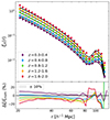 |
Fig. 1. 2PCF of the halos. Top panel: measured (colored dots) and predicted (black lines) 2PCF as a function of the radial separation for different redshift bins. Bottom panel: percent residuals of the model with respect to the numerical function. |
where  is the measured 2PCF averaged over the 1000 simulations, and θinput are the input parameters of the simulations. In this way, we provide an unbiased description of the 2PCF by construction that contains the correct cosmology dependence.
Figure 1 also shows a smaller additional difference both at small separations and around the BAO scale. This difference is due to some nonlinear effects. This confirms that the choice of the radial range is correct. The range cannot be further extended to avoid introducing errors that are due to the limitations of a linear model.
To compute the numerical covariance matrix, we used the estimator
 (22)
(22)
where NS is the number of catalogs,  is the 2PCF in the ath redshift bin and ith radial bin measured from the sth mock, and
  is the corresponding average value. The uncertainty on the numerical covariance is given by (see, e.g., Taylor et al. 2013)
 (23)
(23)
In the upper triangle of Fig. 2, we show the numerical correlation matrix, namely the covariance of Eq. (22) normalized by the diagonal elements
 (24)
(24)
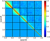 |
Fig. 2. Numerical (upper triangle) and analytical (lower triangle) correlation matrices. The color bar is shown on the right. |
The result confirms the validity of the assumption of negligible cross correlation between redshift bins because the off-block diagonal terms of the matrix are only populated by noise consistent with zero signal. In contrast, inside each redshift bin there is a significant nondiagonal correlation, especially at low redshift.
As a result of the inaccuracy arising from the finite number of simulations, the inverse of this matrix must be corrected as (Anderson 2003; Hartlap et al. 2007)
 (25)
(25)
where ND is the dimension of the data vector. As detailed in Sect. 4.1, our baseline analysis considered five redshift bins and 30 radial bins, that is, ND = 150, which with NS = 1000 gives a correction to the inverse matrix by a factor of ∼0.85.
While this correction removes the bias in the numerical covariance, sampling noise propagates to the parameter covariance, inducing an increase in the error bars by a factor (Taylor et al. 2013; Dodelson & Schneider 2013)
 (26)
(26)
where NP is the number of (cosmological + nuisance) parameters, which we took here to be NP = 2. We obtain f = 1.17, implying an increase of 17% in the parameter error bars due to sampling noise. To reduce this impact to below 10%, the number of mocks must be almost doubled. NS = 2000 would give f = 1.08. This constraint on the number of mocks does not apply when the numerical covariance is fit with a model (Fumagalli et al. 2022), as described in Sect. 4.2. This correction results from a frequentist-style approach concerned with results after repeated trials; for corrections suitable for a Bayesian analysis, the proper approach is described by the works of Sellentin & Heavens (2016), Percival et al. (2022). However, we simply attenuated the propagation of the sampling noise on the parameter constraints by manually setting the cross correlation between redshift bins in the numerical covariance to zero, being dominated entirely by noise. This reduced the number of noise-affected bins in the matrix to ND ∼ Nr = 30, where Nr is the number of radial bins, providing a correction factor for the inverse covariance of ∼0.97 and a negligible increase in the parameter error bars (f ∼ 1.03), allowing us to take the numerical results as reference for the model comparison.
4. Results
In this section we present the results of the covariance comparison and the effect that different covariance configurations have on the cosmological posteriors. In Sect. 4.1 we analyze the redshift and radial binning schemes to determine the configuration that better extracts the information in the likelihood analysis. We then use this configuration for the covariance model validation. In Sect. 4.2, we validate the analytical model, and in Sect. 4.3 we study the impact of the non-Gaussian term on the covariance. Last, in Sect. 4.4 we study the cosmology dependence of the covariance, and in Sect. 4.5 we evaluate the impact of the mass binning.
For the likelihood analysis, we considered the cosmological parameters to which the cluster clustering is more sensitive, that is, Ωm and σ8, or equivalently, As. We assumed flat uninformative priors Ωm ∈ [0.2, 0.4] and log10As ∈ [ − 9.0, − 8.0], and then we derived the value of σ8 through the relation Pm(k) = As kns T2(k), where T(k) is the transfer function, and the definition of variance σ2(R). We are interested in evaluating the variations in the FoM in the Ωm–σ8 plane and the possible biases in the posteriors with respect to the input cosmology.
4.1. Radial and redshift binning
Before starting the model validation, we defined the best binning scheme to properly extract the cosmological information. For this purpose, we performed the likelihood analysis with different combinations of radial and redshift bin widths. For this test, we considered only the covariance matrix extracted from numerical simulations, which is the reference covariance.
We divided the separation range into different numbers of bins: Nr = 20, 25, 30, and 35 log-spaced, plus Nr = 25 linearly spaced, to test the effect of a different spacing. For the redshift binning, we tested three bin widths, Δz = 0.2, 0.4, and 0.5, which properly divide the whole redshift range. We did not consider thinner bins to avoid including non-negligible border effects in the pair-count procedure.
In Fig. 3 we show the FoM for the different numbers of radial bins as a function of the redshift bin width. To take the uncertainty in the inference process into account, we considered the average and the standard error computed over five realizations for each case. We did not observe a significant difference between the various Δz because all the cases agree statistically. About the radial binning, the FoM increases as the number of bins increases, suggesting a more efficient extraction of the information, and it stabilizes around Nr = 30, meaning that no more information can be extracted by increasing the number of radial bins further.
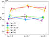 |
Fig. 3. Merit in the Ωm − σ8 plane for different numbers of radial bins as a function of the redshift bin width. A small horizontal displacement has been applied for clarity. |
In the following analyses, we adopt the values Δz = 0.4 and Nr = 30 log-spaced as our baseline redshift and radial bin choice.
4.2. Covariance comparison
In this section, we validate the analytical model of Eq. (12) through the comparison with the numerical matrix. The two correlation matrices are represented in the lower and upper triangle of Fig. 2. For a better comparison, we show in Fig. 4 the diagonal and two off-diagonal terms of the matrices as a function of the radial separation in three redshift bins. The model (solid lines) correctly reproduces the reference values (shaded areas) only at low redshift, while at intermediate and high redshift, it underestimates the numerical matrix by about 30% on the diagonal and by about 50% on the off-diagonal terms. We ascribe this difference to three factors that we list below.
-
Non-Poissonian shot noise: The Poissonian prediction does not describe the shot-noise affecting the halo power spectrum correctly (see Appendix B for further discussion).
-
Inaccurate halo bias: the inaccuracy of the halo bias prediction propagates in the covariance model5;
-
Lack of higher-order terms: The contribution of three- and four-point functions is not negligible. This effect especially regards the terms weighted by
 , which would contribute significantly at high redshift, where the shot noise increases.
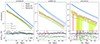 |
Fig. 4. Numerical (shaded areas), analytical (solid lines), and analytical with fitted parameters (dashed lines) covariance matrices as a function of the radial separation in three redshift bins (from left to right: z = 0.0 − 0.4, z = 0.8 − 1.2, z = 1.6 − 2.0). The different colors represent different components of the matrix. The diagonal elements are plotted in blue, the first off-diagonal elements are shown in red, and the second off-diagonal elements are shown in green. The subpanels show the percent residuals of the model covariance with respect to the numerical matrix. |
We corrected the inaccuracy of the predicted covariance by including some parameters in the model. More specifically, we modified Eq. (12) by adding three free parameters {α, β, γ},
![Mathematical equation: $$ \begin{aligned} \begin{aligned} C_{a i j} =&\frac{2}{V_a} \int \frac{{\mathrm{d}} k\,k^2}{2 \pi ^2} \left[ \left\langle ({\beta \, \overline{b}\,})^2P_{\rm m}(k) \right\rangle _a + \left\langle \frac{1 + \alpha }{{\overline{n}}}\right\rangle _a \right]^2 W_i(k) \, W_j(k)\\&+ \frac{2}{V_a V_i} \int \frac{{\mathrm{d}} k\,k^2}{2 \pi ^2} \left\langle ({\beta \, \overline{b}\,})^2 P_{\rm m}(k)\right\rangle _a \left\langle \frac{1+\gamma }{{\overline{n}}}\right\rangle ^2_a \, W_j(k) \ \delta _{ij}, \end{aligned} \end{aligned} $$](/articles/aa/full_html/2024/03/aa45540-22/aa45540-22-eq35.gif) (27)
(27)
where β corrects for the halo bias inaccuracy, and α and γ correct for the non-Poissonian nature of the shot-noise in the main and secondary term, respectively. The different weighting of the shot-noise correction should also account for the effect of higher-order terms. We fit these parameters from simulations in each redshift bin, assuming a constant value with scale and redshift in each slice. We adopted the method described in Fumagalli et al. (2022) to fit the free parameters α, β, and γ. In short, we constrained the covariance by maximizing a Gaussian likelihood evaluated at the fiducial cosmology, with free covariance parameters. The best-fit covariance thus obtained follows a χ2 distribution best with respect to the observed data (we refer to the original paper and to Appendix C for more details of the method). In Table 1 we show the best-fit values of the parameters in each redshift slice6: In most of the cases, the best fit disagrees with the reference values. The correction of the halo bias is in line with the expectation (i.e., β < 1 at low redshift to correct for an overestimated bias, and β > 1 at high redshift to correct for an underestimated bias). At redshift z ≳ 1, the values of β overestimate the 2PCF correction of Eq. (21) by a factor of 5 to 30% depending on redshift. The shot-noise corrections also show contradictory results: The Gaussian term of the covariance seems to prefer a super-Poissonian shot-noise (α > 0), while the non-Gaussian term is characterized by a sub-Poissonian shot-noise (γ < 0). These contrasts suggest that the parameters absorb the effect of the incorrect or missing terms of the covariance instead of simply describing the halo bias correction or the deviation from the Poissonian prediction of the shot noise.
The dashed lines in Fig. 4 show the predictions of the model modified by the introduction of the additional parameters. Now, the analytical covariance correctly describes the numerical results at all redshifts, with an accuracy of about 10%.
In Fig. 5 we show the posterior distributions resulting from the likelihood analysis with three different covariance configurations: numerical, model of Eq. (12) and model of Eq. (27) with the best-fit parameters shown in Table 1. As expected, the underestimated level of the covariance provided by the original model translates into tighter posteriors with respect to the numerical case. In contrast, the model corrected for the additional parameters recovers the result of the numerical matrix well. The FoM obtained from these posteriors and the percent difference with respect to the numerical case are shown in Table 2: The addition of the parameters decreases the deviation in the FoM from ∼40% to only ∼5%.
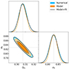 |
Fig. 5. Contour plots at 68 and 95% of the confidence level for the numerical (blue), analytical (model; orange), and analytical with fitted parameters (model+fit; black) matrices. The dotted gray lines represent the fiducial cosmology. |
Merit for the different covariance cases.
4.3. Non-Gaussian term
We tested the effect of the low-order non-Gaussian term (i.e., the second line in Eq. (12)) to evaluate its impact with respect to the Gaussian covariance. In Fig. 6 we compare the numerical matrix with the analytical model, with parameters fitted both from the full model (dashed lines), and from the Gaussian model, that is, setting the non-Gaussian term to zero and fitting α and β (solid lines). Because this term only contributes on the diagonal elements, we compare the variance in three different redshift bins. The figure clearly shows that the Gaussian model is unable to properly describe the numerical covariance for two reasons: First, the non-Gaussian term contributes significantly at small scales, especially at high redshift, and neglecting this term leads to an underestimation of the diagonal terms by a factor up to 50%. Second, the Gaussian model does not have enough degrees of freedom to provide a good fit and is not able to absorb the effect of the missing terms, thus producing an incorrect fit at larger scales as well.
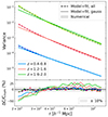 |
Fig. 6. Variance as a function of the radial separation for three redshift bins for the numerical matrix (shaded area), the Gaussian analytical matrix (model+fit, gauss; solid lines), and the full analytical matrix (model+fit, all; dashed lines, corresponding to the dashed lines of Fig. 4). |
The differences observed in the Gaussian fit impact the cosmological posteriors, with deviations in the FoM of about 20% with respect to the numerical covariance case (see Table 2).
The importance of this term is mainly driven by the factor  , which grows with decreasing number of objects. We therefore expect that the impact of this term increases at higher redshifts as well as higher mass-limits. The same trend would apply to the bispectrum terms due to the factor
  , while the trispectum contribution should be less relevant, given the absence of this factor.
4.4. Cosmology dependence
The impact of the cosmology dependence of the covariance on the likelihood analysis has been discussed in literature. Several works (e.g. Krause & Eifler 2017; Eifler et al. 2009; Morrison & Schneider 2013; Blot et al. 2020; Euclid Collaboration 2021) have demonstrated that evaluating the covariance matrix at an incorrect cosmology would lead to an incorrect estimation of the cosmological posteriors. To avoid this, the correct way to perform the parameter inference from a Gaussian likelihood is to use a cosmology-dependent covariance, that is, to recompute the matrix at each step of the MCMC process. The situation becomes more complicated when the Gaussian likelihood is just an approximation of the true distribution of the data, as for the 2PCF. As pointed out by Carron (2013), in this case, the use of a cosmology-dependent covariance may lead to an incorrect estimation of the posterior amplitude. To avoid this, the iterative approach can be used, which consists of running the MCMC with a fixed covariance computed at some fiducial cosmology and then using the best-fit parameters to construct a new covariance matrix and repeating the MCMC process. This can be iterated until convergence of the cosmological posteriors. It should be noted that in the case of approximate likelihood, even this second method may not estimate the posterior amplitude correctly.
Based on this premise, we performed the following test to establish the most correct method for extracting the cosmological information from the 2PCF, with the likelihood and the covariance model proposed in this work. We analyzed 100 light cones in two different ways: (i) We applied the iterative method starting with a fiducial cosmology of Ωm = 0.30 and σ8 = 0.77 and verified that a single step is sufficient to achieve convergence. (ii) We used a cosmology-dependent covariance. For this test, we did not apply Eq. (18) to remove cosmic variance, but analyzed each light cone separately. The left and middle panels of Fig. 7 represent the result of the two analysis: Dots are the best-fit values for each light cone, compared to the mean contours obtained through Eq. (18). The two cases exhibit a different best-fit distribution: The analysis of the light cones with the cosmology-dependent covariance yields values that are more concentrated around the input cosmology than in the fixed covariance case, which instead presents a more scattered distribution. In both cases, the individual values agree with the mean contours, making it difficult to determine which of the two analyses is more correct. Thus, for a better comparison, we computed the deviance information criterion (DIC, Spiegelhalter et al. 2002), treating the problem as a model selection problem. The DIC is defined as
 (28)
(28)
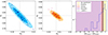 |
Fig. 7. Comparison of 100 light cones analyzed individually with the cosmology-dependent and the fixed-cosmology covariance matrices. Left and middle panels: contour plots at 68 and 95% of the confidence level for input-cosmology covariance (blue) and the cosmology-dependent covariance (orange) obtained from the mean likelihood (Eq. (18)). The dots show the best-fit values from 100 single light cones. The gray lines represent the input parameters. Right panel: ΔDIC distribution of the 100 light cones. The associated mean and the error on the mean are highlighted as solid and dashed black lines. The colored regions represent the Jeffery scale used to interpret the results. |
with
 (29)
(29)
Here, χ2 = −2lnℒ(d|mi(θ),C) estimates the goodness of the fit, and pD is the Bayesian complexity, measuring the effective complexity of the model. The average was performed over the posterior, and θmaxL represents the maximum likelihood point. Given two models m1(θ) and m2(θ), the difference ΔDIC = DIC(m2)−DIC(m1) is interpreted using the Jeffrey scale presented in Grandis et al. (2016): ΔDIC = 0 means that none of the two models is preferred, −2 < ΔDIC < 0 means that there is “no significant” preference for m2, −5 < ΔDIC < −2 means a “positive” preference for m2, −10 < ΔDIC < −5 means a “strong” preference for m2, and ΔDIC < −10 indicates a “decisive” preference for m2. By defining ΔDIC = DICcosmo − DICbestfit for each of the 100 simulations, we obtained the distribution shown in the right panel of Fig. 7, characterized by a mean value ⟨ΔDIC⟩sims = −6.3 ± 0.9. The analysis of the ΔDIC indicates that the model with a cosmology-dependent covariance is statistically strongly preferred over the iterative method. Further considerations are presented in Appendix D.
After verifying that the use of the cosmology-dependence covariance from a statistical point of view is the most correct way to analyze the data, we studied the impact on the (average) cosmological posteriors of an incorrect-cosmology covariance and a cosmology-dependent covariance with respect to the input covariance case. In Fig. 8 we show the posteriors obtained by fixing the covariance matrix at three different cosmologies. More specifically, we compare the input-parameter case (Ωm = 0.307, σ8 = 0.829) with two choices of parameter combinations, that is, Ωm = 0.320, σ8 = 0.775 and Ωm = 0.295, σ8 = 0.871, located approximately at the extremes of the 2σ contours of the input-cosmology posteriors along the degeneracy direction (indicated by dots in the figure, with respect to the orange contours). These deviations from the fiducial cosmology are comparable with the 2σ values from Planck Collaboration VI (2020), which represent the most recent cosmological constraints. A covariance matrix computed at an incorrect cosmology has a strong effect on the cosmological posteriors, with variations in the FoM of ∼30−40%. We note that the recovered posterior distributions differ even when the two adopted cosmologies lie along the Ωm − σ8 degeneracies. This result suggests that the cosmological dependence of the covariance matrix is different from that of the 2PCF.
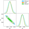 |
Fig. 8. Contour plots at 68 and 95% of the confidence level for the covariance matrix at the input cosmology (orange), compared with two incorrect-cosmology cases: (A) Ωm = 0.320, σ8 = 0.775 in blue, and (B) Ωm = 0.295, σ8 = 0.871 in green. The colored dots indicate the position of the incorrect parameters. The dotted gray lines represent the fiducial cosmology. |
To test this hypothesis, we compared the derived posterior distribution on the cosmological parameters for the following three analyses:
-
(i)
We computed the covariance at the input cosmology and evaluated the expected 2PCF as a function of cosmological parameters. This case corresponds to the standard likelihood analysis with fixed covariance, where all the cosmological information is encapsulated in the expected value of ξ(r, z).
-
(ii)
We evaluated the expected 2PCF at the fixed input cosmology, but let the covariance matrix vary as a function of cosmological parameters. In this way, we evaluated the cosmology dependence of the covariance alone.
-
(iii)
We compared the measured and expected clustering signal where both the mean value and its covariance matrix varied as a function of cosmological parameters. This case corresponds to the full forward-modeling approach.
When adopting a cosmology-dependent covariance, we assumed the fitted parameters α, β, and γ to be cosmology independent. This limitation arises because we only have simulations for one cosmology on which the fit can be performed. The impact of this dependence will be verified in detail in future analyses. However, we expect that neglecting the cosmology dependence of these parameters would introduce a negligible error with respect to the error that we would introduce when these parameters were not included at all.
Figure 9 clearly highlights a tilted degeneracy direction between Ωm and σ8 posteriors of cases (i) and (ii), indicating that covariance and 2PCF have different cosmological dependences (blue versus orange contours). As a result, varying the cosmological parameters in both the quantities returns tighter constraints, with a FoM improved by about 150% with respect to the numerical case, which reflects the standard case (i) likelihood analysis (see Table 2).
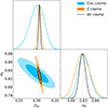 |
Fig. 9. Contour plots at 68 and 95% of the confidence level for three cases: A cosmology-dependent matrix and a fixed mean value (blue), a fixed covariance and a cosmology-dependent mean value (corresponding to the standard analysis; orange), and a cosmology-dependent mean value and a covariance (corresponding to the full cosmology-dependent analysis; black). The dotted gray lines represent the fiducial cosmology. |
This different dependence on cosmology can be explained by noting that unlike the mean value, the covariance of the 2PCF depends on the shot noise, which is proportional to the inverse of the integrated mass function. Letting the cosmology vary in the covariance thus enables us to extract all the information contained in the clustering of the clusters, that is, in addition to the average value of the 2PCF, also the amplitude of its fluctuations provides information. Further considerations about the cosmology dependence of the covariance are presented in Appendices F and E.
4.5. Mass binning
We performed this analysis considering redshift bins of width Δz = 0.5, to allow for more highly populated mass bins. We considered the case of two mass bins with cuts at log10 M/M⊙ = {14.00, 14.15, 16.00}, three mass bins with cuts at log10 M/M⊙ = {14.00, 14.05, 14.15, 16.00}, and four mass bins with cuts at log10 M/M⊙ = {14.00, 14.05, 14.10, 14.20, 16.00}, chosen in order to have at least 4000 objects in each mass and redshift bin.
We show in Fig. 10 the posterior distribution from the three cases with mass binning, compared to the mass threshold case, while in Table 3 we report the corresponding FoMs. We observe an improvement in the FoM when considering the mass binning with respect to the mass-threshold case, indicating that the information included in the halo bias can be exploited in order to obtain tighter constraints on cosmological parameters. However, increasing the number of mass bins does not significantly improve the contours: this can be attributed to the closeness of the bins, characterized by a similar bias relation. On the other hand, selecting more distant bins implies having less populated intervals and therefore noisier quantities.
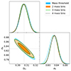 |
Fig. 10. Contour plots at 68 and 95% of the confidence level for three cases: no mass binning (blue), two mass bins (orange), and three mass bins (black). In all the cases, the covariance is given by the numerical matrix. The dotted gray lines represent the fiducial cosmology. |
Merit for the different mass binning cases.
After we established the advantage of considering mass binning, we validated the corresponding covariance model presented in Eq. (16). For greater clarity, we considered the simplest two-mass bins case; the cases with more mass bins are analogous. In Fig. 11 we show the diagonal components of the analytical matrix (solid lines) compared to the corresponding numerical terms (shaded areas). As in the mass threshold case, the model underestimates the expected covariance with a difference in the FoM of about 30% (see Table 3).
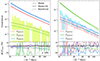 |
Fig. 11. Numerical (shaded areas), analytical (solid lines), and analytical with fitted parameters (dashed lines) covariance matrices as a function of the radial separation in the redshift bin z ∈ [1.0, 1.5]. The different colors represent the diagonal elements of different auto- and cross-correlation components of the matrix. |
Again, we corrected for this discrepancy by adding some covariance parameters, fitted for each mass and redshift bin, according to Eq. (27). When we added the parameters fitted from simulations, the discrepancy between numerical and analytical matrix dropped lower than 5% on the FoM.
Finally, we tested the effect of the cosmology-dependent covariance following the analyses described in Sect. 4.4. In this case, the improvement in the cosmological posteriors was even higher than the mass threshold case. It reached a difference in the FoM of ∼230%. This is due the mass-dependence of the shot-noise, which makes the covariance more constraining than the single-mass threshold case.
5. Discussion and conclusions
We validated a covariance model for the real-space two-point correlation function of galaxy clusters in a survey that is comparable to that expected from the Euclid survey in terms of mass selection, sky coverage, and depth. As this represents a first step in a more complex analysis, we did not account for the effect of selection functions and mass-observable relations.
We considered a Gaussian model plus the low-order non-Gaussian contribution, neglecting high-order terms. This choice was made because we expect the non-Gaussian terms to be minor corrections to the main Gaussian covariance. Great efforts to analytically calculate these complicated terms are therefore not justified computationally. With this premise, we were interested in evaluating the impact of the approximations we made to compute this simple model, that is, the absence of three- and four-point correlation functions, at the level of accuracy required for the future Euclid cluster catalogs.
We validated the covariance model by a comparison with a numerical matrix, estimated by means of 1000 Euclid-like light cones generated with the PINOCCHIO algorithm.
We measured the 2PCF from the light cones with the Landy & Szalay (1993) estimator and compared the result with the theoretical prediction of Eq. (6) in the redshift range z = 0 − 2 and radial range r = 20 − 130 h−1 Mpc. In the first place, we considered halos more massive than Mth = 1014 M⊙. We quantified the differences between covariance matrices by performing a likelihood analysis with different covariance configurations, and evaluating their effect on the cosmological posteriors. To correct for the halo bias inaccuracy in the likelihood analysis, we rescaled the predicted 2PCF to the mean measured 2PCF, plus the cosmology dependence from theory (see Eq. (21)). We constrained the parameters Ωm and σ8, to which the cluster clustering is more strongly sensitive.
The main results of our analysis can be summarized as follows.
-
In Sect. 4.1, we tested different binning schemes to properly extract the cosmological information. We find negligible differences when we varied the width of redshift bins. We also observe a slight increase in the extracted information when the number of radial bins was increased to Nr ≃ 30. We selected the redshift bin width Δz = 0.4 and a number of radial log-spaced bins Nr = 30, corresponding to Δlog10(r/h−1 Mpc) = 0.028.
-
In Sect. 4.2 we compared the analytical model of Eq. (12) with the numerical matrix. The former underestimates the covariance at intermediate and high redshift by ∼30% on the diagonal and ≳50% on the off-diagonal terms. We ascribe this difference to the absence of high-order non-Gaussian terms and to the inaccuracy of the Poissonian shot-noise assumption, as well as to the residual inaccuracy of the assumed model for the halo bias.
-
We improved the model by adding three parameters {α, β, γ} to correct for non-Poissonian shot-noise and halo bias prediction, as well as to absorb the effect of the missing high-order terms. The parameters were fit from simulations. We obtained an agreement within 10% with the numerical matrix at all the redshifts. Even when the missing terms were added analytically and a perfect description of the halo bias was provided, the exact value of the shot noise could not be predicted. Correcting the model with these fitted parameters is therefore a well-motivated procedure.
-
From the likelihood analysis, we find that using the analytical covariance model produces a difference of ∼40% on the cosmological FoM with respect to the numerical covariance. This difference drops to ∼5% when the fitted parameters are added to the model. This difference is considered to be negligible in more complete analyses (e.g., richness-selected catalogs), where it is most likely to be absorbed by the broadening of the cosmological posteriors.
-
In Sect. 4.3 we assessed the relevance of the low-order non-Gaussian term, which was non-negligible at small scales, especially at high redshift.
-
In Sect. 4.4 we find that in this analysis, the likelihood with cosmology-dependent covariance is statistically preferred over the iterative method. We also find that evaluating the covariance at a fixed incorrect cosmology can lead to an under/overestimated posterior amplitude. Moreover, neglecting the cosmology dependence of the covariance means losing the information contained in the shot-noise term. This information is not contained directly in the 2PCF, but is nevertheless information that characterizes the clustering of clusters.
-
In Sect. 4.5 we assessed the cosmological information encoded in the shape of the halo bias by splitting our sample into mass bins, finding a significant improvement in the FoM compared to the mass-threshold case. This improvement is expected to be even stronger for richness-selected halos, where this dependence can help us to constrain the mass-observable relation parameters in addition to the cosmological ones.
Two main results emerge from this analysis. First, a pure Gaussian model is not sufficient for cluster clustering to correctly describe the covariance. This is due to the low number densities that characterize the spatial distribution of these objects, making non-Gaussian terms more important as the redshift and the mass threshold increase. Despite this, a simple semi-analytical model with parameters fitted from simulations permits us to correct the inaccuracy of the model and gives an accurate estimate of the errors associated with the 2PCF. Although this model still requires the use of simulations to fit the covariance parameters, the number of simulations is considerably lower than the number required to compute a good numerical matrix, i.e., approximately O(102) instead of O(103). Furthermore, the resulting matrix is completely noise free and accounts for the dependence on cosmological parameters.
Second, the covariance of the 2PCF contains cosmological information that is not present in the mean value. Therefore, both quantities should be taken into account in constraining cosmological parameters to correctly extract the information enclosed in the cluster clustering, especially when the mass binning is included. This may require some care when performing a combined analysis of cluster number counts and cluster clustering because the cosmological information contained in the 2PCF covariance is also contained in the number counts. We reserve an examination of this issue in detail for a future dedicated work.
We showed that a simple semi-analytical model can be used to accurately describe the cluster-clustering covariance matrix. However, the calibration of this model is not universal, but depends on the specific properties of the survey, such as the geometry or the mass and redshift range. The fit of the covariance parameters must then be performed for each survey in appropriate simulations. Moreover, these parameters may contain a non-negligible dependence on cosmology, whose impact is still to be quantified.
Finally, we note that in a cluster-clustering analysis of observed cluster samples, the uncertainties on the calibration of the mass-observable relations represent a major (and often dominant) systematic. The comprehensive characterization of the model presented in this work together with the a self-consistent treatment of the mass calibration and calibration of the selection function will be presented in a forthcoming paper. Moreover, the calibration described in this work only holds for a ΛCDM Universe; further analysis is thus required to validate the model in nonstandard cosmological models. When a complete description of the 2PCF and its covariance are obtained, it will be possible to exploit the clustering of galaxy clusters to obtain cosmological constraints and to assess its impact on the combined analysis with other cosmological observables at the level of accuracy that will be achieved by Euclid.
This expression is valid for a conical geometry survey; in more generic cases, the integral over the lightcone volume must take into account the geometry of the survey.
The light cones can be obtained on request. The list of the available mocks can be found at http://adlibitum.oats.inaf.it/monaco/mocks.html; the light cones we analyzed are labeled “NewClusterMocks”.
Our light cones cover slightly smaller areas than the expected Euclid catalogs (∼10 000 vs. ∼15 000 deg2); the survey will also cover two separate patches of the sky. For the purpose of this work, we expect that these differences impact the results in a negligible way.
The correction of Eq. (21) does not apply to the covariance prediction. However, this does not affect the following results because we treated the bias in the 2PCF and the bias in the covariance model as two different quantities.
We show the value of best-fit parameters for general considerations. However, the value of these parameters is not universal, but depends on the properties of the survey and must be fit for each specific case.
Acknowledgments
We thank an anonymous referee for making helpful suggestions to improve the quality of the paper. A.F., A.S., T.C. and S.B. are supported by the INFN INDARK PD51 grant. A.F., M.C., and A.S. are also supported by the ERC “ClustersXCosmo” grant agreement 716762. T.C. and A.S. are also supported by the FARE MIUR grant “ClustersXEuclid” R165SBKTMA. This work has been supported by the grant ASI n.2018-23-HH.0. The Euclid Consortium acknowledges the European Space Agency and a number of agencies and institutes that have supported the development of Euclid, in particular the Academy of Finland, the Agenzia Spaziale Italiana, the Belgian Science Policy, the Canadian Euclid Consortium, the French Centre National d’Etudes Spatiales, the Deutsches Zentrum für Luft- und Raumfahrt, the Danish Space Research Institute, the Fundação para a Ciência e a Tecnologia, the Ministerio de Ciencia e Innovación, the National Aeronautics and Space Administration, the National Astronomical Observatory of Japan, the Netherlandse Onderzoekschool Voor Astronomie, the Norwegian Space Agency, the Romanian Space Agency, the State Secretariat for Education, Research and Innovation (SERI) at the Swiss Space Office (SSO), and the United Kingdom Space Agency. A complete and detailed list is available on the Euclid website (http://www.euclid-ec.org).
References
- Albrecht, A., Bernstein, G., Cahn, R., et al. 2006, arXiv e-prints [arXiv:astro-ph/0609591] [Google Scholar]
- Anderson, T. 2003, An Introduction to Multivariate Statistical Analysis, Wiley Series in Probability and Statistics (Wiley) [Google Scholar]
- Angulo, R., Baugh, C. M., Frenk, C. S., et al. 2005, MNRAS, 362, L25 [NASA ADS] [CrossRef] [Google Scholar]
- Baldauf, T., Mirbabayi, M., Simonović, M., & Zaldarriaga, M. 2015, Phys. Rev. D, 92, 043514 [NASA ADS] [CrossRef] [Google Scholar]
- Bernstein, G. M. 1994, ApJ, 424, 569 [NASA ADS] [CrossRef] [Google Scholar]
- Blot, L., Crocce, M., Sefusatti, E., et al. 2019, MNRAS, 485, 2806 [NASA ADS] [CrossRef] [Google Scholar]
- Blot, L., Corasaniti, P.-S., Rasera, Y., & Agarwal, S. 2020, MNRAS, 500, 2532 [NASA ADS] [CrossRef] [Google Scholar]
- Bond, J. R., & Myers, S. T. 1996, ApJS, 103, 1 [NASA ADS] [CrossRef] [Google Scholar]
- Borgani, S., Plionis, M., & Kolokotronis, E. 1999, MNRAS, 305, 866 [NASA ADS] [CrossRef] [Google Scholar]
- Bouchet, F. R., Colombi, S., Hivon, E., & Juszkiewicz, R. 1995, A&A, 296, 575 [NASA ADS] [Google Scholar]
- Buchert, T. 1992, MNRAS, 254, 729 [NASA ADS] [CrossRef] [Google Scholar]
- Buchner, J., Georgakakis, A., Nandra, K., et al. 2014, A&A, 564, A125 [NASA ADS] [CrossRef] [EDP Sciences] [Google Scholar]
- Carron, J. 2013, A&A, 551, A88 [NASA ADS] [CrossRef] [EDP Sciences] [Google Scholar]
- Castro, T., Borgani, S., Dolag, K., et al. 2020, MNRAS, 500, 2316 [Google Scholar]
- Cohn, J. D. 2006, New Astron., 11, 226 [NASA ADS] [CrossRef] [Google Scholar]
- Colavincenzo, M., Sefusatti, E., Monaco, P., et al. 2019, MNRAS, 482, 4883 [NASA ADS] [CrossRef] [Google Scholar]
- Cole, S., Percival, W. J., Peacock, J. A., et al. 2005, MNRAS, 362, 505 [Google Scholar]
- Despali, G., Giocoli, C., Angulo, R. E., et al. 2016, MNRAS, 456, 2486 [NASA ADS] [CrossRef] [Google Scholar]
- Dodelson, S., & Schneider, M. D. 2013, Phys. Rev. D, 88, 063537 [Google Scholar]
- Eifler, T., Schneider, P., & Hartlap, J. 2009, A&A, 502, 721 [NASA ADS] [CrossRef] [EDP Sciences] [Google Scholar]
- Eisenstein, D. J., & Loeb, A. 1995, ApJ, 439, 520 [NASA ADS] [CrossRef] [Google Scholar]
- Eisenstein, D. J., Zehavi, I., Hoggand, D. W., et al. 2005, ApJ, 633, 560 [NASA ADS] [CrossRef] [Google Scholar]
- Eisenstein, D. J., Seo, H.-J., Sirko, E., & Spergel, D. 2007, ApJ, 664, 675 [NASA ADS] [CrossRef] [Google Scholar]
- Estrada, J., Sefusatti, E., & Frieman, J. A. 2009, ApJ, 692, 265 [NASA ADS] [CrossRef] [Google Scholar]
- Euclid Collaboration (Fumagalli, A., et al.) 2021, A&A, 652, A21 [NASA ADS] [CrossRef] [EDP Sciences] [Google Scholar]
- Euclid Collaboration (Scaramella, R., et al.) 2022, A&A, 662, A112 [NASA ADS] [CrossRef] [EDP Sciences] [Google Scholar]
- Feldman, H. A., Kaiser, N., & Peacock, J. A. 1994, ApJ, 426, 23 [Google Scholar]
- Friedrich, O., Seitz, S., Eifler, T. F., & Gruen, D. 2016, MNRAS, 456, 2662 [NASA ADS] [CrossRef] [Google Scholar]
- Fumagalli, A., Biagetti, M., Saro, A., et al. 2022, JCAP, 2022, 022 [CrossRef] [Google Scholar]
- Grandis, S., Rapetti, D., Saro, A., Mohr, J. J., & Dietrich, J. P. 2016, MNRAS, 463, 1416 [NASA ADS] [CrossRef] [Google Scholar]
- Hartlap, J., Simon, P., & Schneider, P. 2007, A&A, 464, 399 [NASA ADS] [CrossRef] [EDP Sciences] [Google Scholar]
- Hu, W., & Jain, B. 2004, Phys. Rev. D, 70, 043009 [Google Scholar]
- Hu, W., & Kravtsov, A. V. 2003, ApJ, 584, 702 [Google Scholar]
- Huetsi, G. 2010, MNRAS, 401, 2477 [CrossRef] [Google Scholar]
- Kerscher, M., Szapudi, I., & Szalay, A. S. 2000, ApJ, 535, L13 [NASA ADS] [CrossRef] [Google Scholar]
- Krause, E., & Eifler, T. 2017, MNRAS, 470, 2100 [NASA ADS] [CrossRef] [Google Scholar]
- Kravtsov, A., & Borgani, S. 2012, ARA&A, 50, 353 [NASA ADS] [CrossRef] [Google Scholar]
- Lacasa, F., & Kunz, M. 2017, A&A, 604, A104 [NASA ADS] [CrossRef] [EDP Sciences] [Google Scholar]
- Landy, S. D., & Szalay, A. S. 1993, ApJ, 412, 64 [Google Scholar]
- Laureijs, R., Amiaux, J., Arduini, S., et al. 2011, arXiv e-prints [arXiv:1110.3193] [Google Scholar]
- Lesci, G. F., Nanni, L., Marulli, F., et al. 2022, A&A, 665, A100 [NASA ADS] [CrossRef] [EDP Sciences] [Google Scholar]
- Lewis, A., Challinor, A., & Lasenby, A. 2000, ApJ, 538, 473 [Google Scholar]
- Li, Y., Singh, S., Yu, B., Feng, Y., & Seljak, U. 2019, JCAP, 01, 016 [NASA ADS] [Google Scholar]
- Lippich, M., Sánchez, A. G., Colavincenzo, M., et al. 2019, MNRAS, 482, 1786 [NASA ADS] [CrossRef] [Google Scholar]
- Majumdar, S., & Mohr, J. J. 2004, ApJ, 613, 41 [NASA ADS] [CrossRef] [Google Scholar]
- Mana, A., Giannantonio, T., Weller, J., et al. 2013, MNRAS, 434, 684 [NASA ADS] [CrossRef] [Google Scholar]
- Manera, M., Sheth, R. K., & Scoccimarro, R. 2010, MNRAS, 402, 589 [NASA ADS] [CrossRef] [Google Scholar]
- Marulli, F., Veropalumbo, A., & Moresco, M. 2016, Astron. Comput., 14, 35 [Google Scholar]
- Marulli, F., Veropalumbo, A., Sereno, M., et al. 2018, A&A, 620, A1 [NASA ADS] [CrossRef] [EDP Sciences] [Google Scholar]
- Marulli, F., Veropalumbo, A., García-Farieta, J. E., et al. 2021, ApJ, 920, 13 [Google Scholar]
- Meiksin, A., & White, M. J. 1999, MNRAS, 308, 1179 [NASA ADS] [CrossRef] [Google Scholar]
- Miller, C. J., Nichol, R. C., & Batuski, D. J. 2001, ApJ, 555, 68 [NASA ADS] [CrossRef] [Google Scholar]
- Mo, H. J., & White, S. D. M. 1996, MNRAS, 282, 347 [Google Scholar]
- Mohammad, F. G., & Percival, W. J. 2022, MNRAS, 514, 1289 [NASA ADS] [CrossRef] [Google Scholar]
- Monaco, P. 2016, Galaxies, 4, 53 [NASA ADS] [CrossRef] [Google Scholar]
- Monaco, P., Theuns, T., & Taffoni, G. 2002, MNRAS, 331, 587 [Google Scholar]
- Moresco, M., Veropalumbo, A., Marulli, F., Moscardini, L., & Cimatti, A. 2021, ApJ, 919, 144 [NASA ADS] [CrossRef] [Google Scholar]
- Morrison, C. B., & Schneider, M. D. 2013, JCAP, 11, 009 [CrossRef] [Google Scholar]
- Moscardini, L., Matarrese, S., Lucchin, F., & Rosati, P. 2000, MNRAS, 316, 283 [CrossRef] [Google Scholar]
- Moutarde, F., Alimi, J. M., Bouchet, F. R., Pellat, R., & Ramani, A. 1991, ApJ, 382, 377 [Google Scholar]
- Munari, E., Monaco, P., Sefusatti, E., et al. 2017, MNRAS, 465, 4658 [Google Scholar]
- Norberg, P., Baugh, C. M., Gaztanaga, E., & Croton, D. J. 2009, MNRAS, 396, 19 [NASA ADS] [CrossRef] [Google Scholar]
- O’Connell, R., Eisenstein, D., Vargas, M., Ho, S., & Padmanabhan, N. 2016, MNRAS, 462, 2681 [CrossRef] [Google Scholar]
- Paech, K., Hamaus, N., Hoyle, B., et al. 2017, MNRAS, 470, 2566 [NASA ADS] [CrossRef] [Google Scholar]
- Percival, W. J., Friedrich, O., Sellentin, E., & Heavens, A. 2022, MNRAS, 510, 3207 [NASA ADS] [CrossRef] [Google Scholar]
- Philcox, O. H. E., & Eisenstein, D. J. 2019, MNRAS, 490, 5931 [NASA ADS] [CrossRef] [Google Scholar]
- Planck Collaboration XVI. 2014, A&A, 571, A16 [NASA ADS] [CrossRef] [EDP Sciences] [Google Scholar]
- Planck Collaboration VI. 2020, A&A, 641, A6 [Erratum: A&A 652, C4 (2021)] [NASA ADS] [CrossRef] [EDP Sciences] [Google Scholar]
- Pope, A. C., & Szapudi, I. 2008, MNRAS, 389, 766 [NASA ADS] [CrossRef] [Google Scholar]
- Pratt, G. W., Arnaud, M., Biviano, A., et al. 2019, Space Sci. Rev., 215, 25 [Google Scholar]
- Sahni, V., & Coles, P. 1995, Phys. Rep., 262, 1 [Google Scholar]
- Sartoris, B., Biviano, A., Fedeli, C., et al. 2016, MNRAS, 459, 1764 [Google Scholar]
- Schuecker, P., Bohringer, H., Collins, C. A., & Guzzo, L. 2003, A&A, 398, 867 [NASA ADS] [CrossRef] [EDP Sciences] [Google Scholar]
- Scoccimarro, R., Zaldarriaga, M., & Hui, L. 1999, ApJ, 527, 1 [NASA ADS] [CrossRef] [Google Scholar]
- Sellentin, E., & Heavens, A. F. 2016, MNRAS, 456, L132 [Google Scholar]
- Senatore, L., & Zaldarriaga, M. 2015, JCAP, 02, 013 [NASA ADS] [CrossRef] [Google Scholar]
- Sereno, M., Veropalumbo, A., Marulli, F., et al. 2015, MNRAS, 449, 4147 [NASA ADS] [CrossRef] [Google Scholar]
- Smith, R. E. 2009, MNRAS, 400, 851 [NASA ADS] [CrossRef] [Google Scholar]
- Spiegelhalter, D. J., Best, N. G., Carlin, B. P., & van der Linde, A. 2002, J. R. Stat. Soc. B, 64, 583 [Google Scholar]
- Takada, M., & Hu, W. 2013, Phys. Rev. D, 87, 123504 [NASA ADS] [CrossRef] [Google Scholar]
- Taylor, A., Joachimi, B., & Kitching, T. 2013, MNRAS, 432, 1928 [Google Scholar]
- Tinker, J. L., Robertson, B. E., Kravtsov, A. V., et al. 2010, ApJ, 724, 878 [NASA ADS] [CrossRef] [Google Scholar]
- To, C.-H., Krause, E., Rozo, E., et al. 2021a, Phys. Rev. Lett., 126, 141301 [NASA ADS] [CrossRef] [Google Scholar]
- To, C.-H., Krause, E., Rozo, E., et al. 2021b, MNRAS, 502, 4093 [NASA ADS] [CrossRef] [Google Scholar]
- Valageas, P., Clerc, N., Pacaud, F., & Pierre, M. 2011, A&A, 536, A95 [NASA ADS] [CrossRef] [EDP Sciences] [Google Scholar]
- Veropalumbo, A., Marulli, F., Moscardini, L., Moresco, M., & Cimatti, A. 2014, MNRAS, 442, 3275 [NASA ADS] [CrossRef] [Google Scholar]
- Wadekar, D., & Scoccimarro, R. 2020, Phys. Rev. D, 102, 123517 [NASA ADS] [CrossRef] [Google Scholar]
- Xu, X., Padmanabhan, N., Eisenstein, D. J., Mehta, K. T., & Cuesta, A. J. 2012, MNRAS, 427, 2146 [NASA ADS] [CrossRef] [Google Scholar]
Appendix A: Cross-correlation covariance
We generalize here the expression for the covariance of the cross-power spectrum of different tracers proposed by Smith (2009, Section 3, and Equation 43 specifically), accounting for the cross correlation of four tracers (mass bins in our case) A, B, C, and D. Similarly to Eq. (9), we define the covariance of the cross-power spectrum as
![Mathematical equation: $$ \begin{aligned} C_{ABCD}(\mathbf k _1,\mathbf k _2) = \left\langle \left[\hat{P}_{AB}(\mathbf k _1) - \langle \hat{P}_{AB}(\mathbf k _1) \rangle \right] \left[ \hat{P}_{CD}(\mathbf k _2) - \langle \hat{P}_{CD}(\mathbf k _2) \rangle \right] \right\rangle . \end{aligned} $$](/articles/aa/full_html/2024/03/aa45540-22/aa45540-22-eq40.gif) (A.1)
(A.1)
Substituting the definition of the estimator for the halo cross-power spectrum,
 (A.2)
(A.2)
we obtain
 (A.3)
(A.3)
The first term is the cross trispectrum,
 (A.4)
(A.4)
where NAi is the number of A-type halos (or halos in the Ath mass bin) at position vector ri.
Performing the calculations analogously to those shown in Sect. 3 of Smith (2009), we obtain the final expression for the cross-power spectrum covariance,
![Mathematical equation: $$ \begin{aligned} \begin{aligned} C_{ABCD}&(\mathbf k _1,\mathbf k _2) = \frac{1}{V}\, T_{ABCD}(\mathbf k _1,-\mathbf k _1,\mathbf k _2,-\mathbf k _2)\\&+ \left( P_{AC}+\frac{\delta ^\mathrm{K}_{AC}}{\overline{n}_{A}}\right)\,\left( P_{BD}+\frac{\delta ^\mathrm{K}_{BD}}{\overline{n}_{B}}\right)\,\delta ^\mathrm{K}(\mathbf k _1+\mathbf k _2)\\&+ \left( P_{AD}+\frac{\delta ^\mathrm{K}_{AD}}{\overline{n}_{A}}\right)\,\left( P_{BC}+\frac{\delta ^\mathrm{K}_{BC}}{\overline{n}_{B}}\right)\,\delta ^\mathrm{K}(\mathbf k _1-\mathbf k _2)\\&+ \frac{\delta ^\mathrm{K}_{AC}}{\overline{n}_A\,V}\, B_{BDA}(\mathbf k _1,\mathbf k _2) + \frac{\delta ^\mathrm{K}_{AD}}{\overline{n}_A\,V}\, B_{BCA}(\mathbf k _1,-\mathbf k _2)\\&+ \frac{\delta ^\mathrm{K}_{BC}}{\overline{n}_B\,V}\, B_{ADB}(\mathbf k _1,-\mathbf k _2) + \frac{\delta ^\mathrm{K}_{BD}}{\overline{n}_B\,V}\, B_{ACB}(\mathbf k _1,\mathbf k _2)\\&+ \frac{\delta ^\mathrm{K}_{CD}}{\overline{n}_C\,V}\, B_{ABC}(\mathbf k _1,-\mathbf k _1,0) + \frac{\delta ^\mathrm{K}_{AB}}{\overline{n}_A\,V}\, B_{CDA}(\mathbf k _2,-\mathbf k _2,0)\\&+ \frac{\delta ^\mathrm{K}_{AC}\,\delta ^\mathrm{K}_{BD}}{\overline{n}_A\,\overline{n}_B\,V}\,P_{AB}(\mathbf k _1+\mathbf k _2) + \frac{\delta ^\mathrm{K}_{AD}\,\delta ^\mathrm{K}_{BC}}{\overline{n}_A\,\overline{n}_B\,V}\,P_{AB}(\mathbf k _1-\mathbf k _2)\\&+ \frac{\delta ^\mathrm{K}_{AB}\,\delta ^\mathrm{K}_{CD}}{\overline{n}_A\,\overline{n}_C\,V}\,P_{AC}(0) +\frac{1}{\overline{n}^3_A\,V}\,\delta ^\mathrm{K}_{AB}\,\delta ^\mathrm{K}_{BC}\,\delta ^\mathrm{K}_{CD}\\&+ \frac{1}{\overline{n}^2_A\,V}\,\bigg [ \delta ^\mathrm{K}_{AB}\,\delta ^\mathrm{K}_{BC}\,P_{AC}(k_2) + \delta ^\mathrm{K}_{AB}\,\delta ^\mathrm{K}_{BD}\,P_{AC}(k_2)\\&+ \delta ^\mathrm{K}_{AC}\,\delta ^\mathrm{K}_{CD}\,P_{AB}(k_1) + \delta ^\mathrm{K}_{BC}\,\delta ^\mathrm{K}_{CD}\,P_{AB}(k_1) \bigg ]. \end{aligned} \end{aligned} $$](/articles/aa/full_html/2024/03/aa45540-22/aa45540-22-eq44.gif) (A.5)
(A.5)
In case of a single tracer (A = B = C = D), the above expression recovers the standard covariance given by Eq. (11).
By Fourier transforming Eq. (A.5), integrating over separation and redshift bins, and neglecting the high-order terms, we obtain the expression for the cross-2PCF covariance of different tracers (Eq. 16).
Appendix B: Non-Poissonian shot noise
To better assess the impact of shot-noise and its deviation from the Poissonian prediction, we studied the power spectrum, that is, the quantity that is directly affected by this correction. To avoid complications due to the redshift integration and the geometry of the survey, we measured the power spectrum from 1000 cubical boxes of size L = 3870 h−1 Mpc with the same properties and cosmology of the light cones described in Sect. 3.1. We considered three redshifts z = 0.5, 1.0, and 1.5.
We computed the analytical total halo power spectrum as
 (B.1)
(B.1)
where the matter power spectrum wads calculated by means of the CAMB code (Lewis et al. 2000). We compared this quantity with the measured total power spectrum averaged over the 1000 boxes for the three redshift values.
In Fig. B.1 we show the comparison of the measured and predicted power spectra (to facilitate comparison, we show the halo power spectrum, i.e., the total spectrum minus the shot noise): while at low redshift the two quantities agree on almost all the scales, they clearly deviate between the observed and predicted spectra, which increase with redshift to more than 20%. We tried to correct these discrepancies by fitting the two parameters {α, β}, which account for the correction to shot noise and halo bias, respectively, directly from the power spectrum; the best fits are shown in Table B.1 and the resulting power spectra are shown in Fig. B.1 (dotted lines). We obtain an agreement of the fitted power spectra within the 5% level at all the linear scales at all redshifts. Nevertheless, the values deviate by several σ from the best-fit parameters found from the covariance fit in the corresponding redshift intervals (see Table 1). This confirms that the parameters in the covariance, in addition to correct for the incorrect prediction of bias and shot noise, also absorb the effect of the missing higher-order terms in the model.
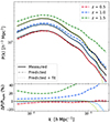 |
Fig. B.1. Halo power spectrum. Top panel: Measured (solid black lines), predicted (dashed darker lines), and fitted (dotted lighter lines) halo power spectrum for boxes at three different redshifts. Bottom panel: Percent residuals of the predictions with respect to the measured residuals. |
Best-fit parameters for the power spectrum parameters.
Appendix C: Covariance parameter fit
We show here the results of the covariance parameters fit, following the method proposed in Fumagalli et al. (2022). In Fig. C.1 we show the χ2 distributions computed with respect to the measurements from the 1000 light cones for the three covariance matrices. In Table C.1 we report the mean and standard deviation for each distribution, with the corresponding 1σ uncertainties computed with the bootstrap technique. By construction, we expect the numerical matrix to perfectly follow the reference distribution. While this is true for the mean value, the variance differs by ∼4σ from the expected value; this discrepancy is ascribed to the noise in the numerical matrix that tightens the distribution. Because the errors are quite small, this distribution can be considered to agree well with the expected one. Instead, the model of Eq. (12) produces a distribution that is several σ different from the expectation, confirming that this model is not suitable for describing the covariance of the data. Finally, the fitted matrix agrees well with the reference distribution for the mean value and the variance. This proves the goodness of our fit and ensures that the resulting model is able to correctly describe the covariance as well as if not better than the numerical matrix. The fitting process provides consistent results when the fit is performed with only 100 simulations.
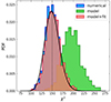 |
Fig. C.1. χ2 distribution for the numerical, analytical, and analytical with fitted parameters covariance matrices. The reference distribution is plotted in black. |
χ2distribution test values.
Appendix D: Cosmology-dependent matrix
To further explore the comparison between the fully cosmology-dependent likelihood analysis and the iterative method, we generated 100 synthetic light cones starting from a Gaussian distribution, with the amplitude given by the covariance model at the input cosmology. In this way, we ensured that the Gaussian distribution was the true likelihood describing the data and not just an approximation. We repeated the analysis of the 100 light cones described in Sect. 4.4, finding a mean value ⟨ΔDIC⟩synth = −8.4 ± 1.7, to be compared with the value from the analysis of the 100 PINOCCHIO mocks, that is, ⟨ΔDIC⟩sims = −6.3 ± 0.9. Moreover, by comparing the FoM of the cosmology-dependent covariance and the iterative method, we obtain a mean variation of ⟨ΔFoM⟩synth = 176 ± 38% for the synthetic catalogs and ⟨ΔFoM⟩sims = 142 ± 33% for the PINOCCHIO mocks. Both the DIC and the FoM analyses indicate that the two analysis are fully consistent. Although this result still does not define which posteriors are correct when the true likelihood is unknown, it shows that at least for this particular analysis, the narrowing of the posteriors does not primarily depend on some incorrect approximation of the likelihood function. In other words, when a Gaussian likelihood is assumed, it is possible to extract information from the cosmology dependence of the covariance.
Appendix E: Cosmology dependence of the number count covariance
We discuss here some additional considerations about the cosmology dependence of the covariance, using as an example the cluster number counts. It has been shown in Euclid Collaboration (2021) that the use of a fixed covariance in the likelihood analysis can bring an under/overestimation of the FoM by more than 40%, if the cosmology at which the covariance is evaluated deviates from the fiducial values of an amount of 2σ from Planck Collaboration VI (2020). Instead, the input and varying covariance cases do not vary significantly. We performed the same test on the cosmology dependence of the covariance described in Sect. 4.4, obtaining the posteriors shown in Fig. E.1. Unlike for the clustering case, for the number counts, the mean value is much more constraining than its covariance, making the degeneracy direction of the latter totally irrelevant. In this case, the covariance thus only contributes as an estimation of the uncertainty, without adding further independent information.
Appendix F: Mass dependence of the covariance
In Fig. F.1 we show the different diagonal contribution to the covariance, composing the model of Eq. (12). The components of the model show a different dependence on the mass threshold, which drastically changes the impact of the various contributions. While at the high-mass threshold, the number density is low, making the shot-noise terms dominant, at low-mass cuts, this contribution is much lower than that from the halo power spectrum.
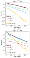 |
Fig. F.1. Diagonal contributions to the covariance matrix composing the model of Eq. (12). The red, green, and blue lines represent the three terms of the Gaussian covariance, and the yellow line is the non-Gaussian term. The comparison is shown for two different mass thresholds: a low-mass threshold Mth = 1 × 10¹³ M⊙ in the top panel, and a high-mass threshold Mth = 1 × 10¹⁴ M⊙ in the bottom panel. The terms are obtained by evaluating the covariance model at the input cosmology in the redshift bin z = 0.8 − 1.2. |
This mass dependence has an important consequence when considering the cosmology dependence of the covariance: Because the additional information extracted from the covariance is mainly given by the shot-noise term, we expect the impact of the cosmology-dependent covariance to be negligible when considering low-mass objects. In other words, the results shown in this work only hold for cluster clustering, while they would not have any substantial impact on galaxy clustering. Moreover, the results shown here consider the ideal case of a simple mass cut; this may vary in real surveys, where selection functions set a mass- and redshift-dependent richness threshold. The study of the impact of the covariance in real observable conditions is left for a future work.
All Tables
All Figures
|
Fig. 1. 2PCF of the halos. Top panel: measured (colored dots) and predicted (black lines) 2PCF as a function of the radial separation for different redshift bins. Bottom panel: percent residuals of the model with respect to the numerical function. |
| In the text | |
|
Fig. 2. Numerical (upper triangle) and analytical (lower triangle) correlation matrices. The color bar is shown on the right. |
| In the text | |
|
Fig. 3. Merit in the Ωm − σ8 plane for different numbers of radial bins as a function of the redshift bin width. A small horizontal displacement has been applied for clarity. |
| In the text | |
|
Fig. 4. Numerical (shaded areas), analytical (solid lines), and analytical with fitted parameters (dashed lines) covariance matrices as a function of the radial separation in three redshift bins (from left to right: z = 0.0 − 0.4, z = 0.8 − 1.2, z = 1.6 − 2.0). The different colors represent different components of the matrix. The diagonal elements are plotted in blue, the first off-diagonal elements are shown in red, and the second off-diagonal elements are shown in green. The subpanels show the percent residuals of the model covariance with respect to the numerical matrix. |
| In the text | |
|
Fig. 5. Contour plots at 68 and 95% of the confidence level for the numerical (blue), analytical (model; orange), and analytical with fitted parameters (model+fit; black) matrices. The dotted gray lines represent the fiducial cosmology. |
| In the text | |
|
Fig. 6. Variance as a function of the radial separation for three redshift bins for the numerical matrix (shaded area), the Gaussian analytical matrix (model+fit, gauss; solid lines), and the full analytical matrix (model+fit, all; dashed lines, corresponding to the dashed lines of Fig. 4). |
| In the text | |
|
Fig. 7. Comparison of 100 light cones analyzed individually with the cosmology-dependent and the fixed-cosmology covariance matrices. Left and middle panels: contour plots at 68 and 95% of the confidence level for input-cosmology covariance (blue) and the cosmology-dependent covariance (orange) obtained from the mean likelihood (Eq. (18)). The dots show the best-fit values from 100 single light cones. The gray lines represent the input parameters. Right panel: ΔDIC distribution of the 100 light cones. The associated mean and the error on the mean are highlighted as solid and dashed black lines. The colored regions represent the Jeffery scale used to interpret the results. |
| In the text | |
|
Fig. 8. Contour plots at 68 and 95% of the confidence level for the covariance matrix at the input cosmology (orange), compared with two incorrect-cosmology cases: (A) Ωm = 0.320, σ8 = 0.775 in blue, and (B) Ωm = 0.295, σ8 = 0.871 in green. The colored dots indicate the position of the incorrect parameters. The dotted gray lines represent the fiducial cosmology. |
| In the text | |
|
Fig. 9. Contour plots at 68 and 95% of the confidence level for three cases: A cosmology-dependent matrix and a fixed mean value (blue), a fixed covariance and a cosmology-dependent mean value (corresponding to the standard analysis; orange), and a cosmology-dependent mean value and a covariance (corresponding to the full cosmology-dependent analysis; black). The dotted gray lines represent the fiducial cosmology. |
| In the text | |
|
Fig. 10. Contour plots at 68 and 95% of the confidence level for three cases: no mass binning (blue), two mass bins (orange), and three mass bins (black). In all the cases, the covariance is given by the numerical matrix. The dotted gray lines represent the fiducial cosmology. |
| In the text | |
|
Fig. 11. Numerical (shaded areas), analytical (solid lines), and analytical with fitted parameters (dashed lines) covariance matrices as a function of the radial separation in the redshift bin z ∈ [1.0, 1.5]. The different colors represent the diagonal elements of different auto- and cross-correlation components of the matrix. |
| In the text | |
|
Fig. B.1. Halo power spectrum. Top panel: Measured (solid black lines), predicted (dashed darker lines), and fitted (dotted lighter lines) halo power spectrum for boxes at three different redshifts. Bottom panel: Percent residuals of the predictions with respect to the measured residuals. |
| In the text | |
|
Fig. C.1. χ2 distribution for the numerical, analytical, and analytical with fitted parameters covariance matrices. The reference distribution is plotted in black. |
| In the text | |
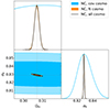 |
Fig. E.1. Same as Fig. 9 for cluster number counts. |
| In the text | |
|
Fig. F.1. Diagonal contributions to the covariance matrix composing the model of Eq. (12). The red, green, and blue lines represent the three terms of the Gaussian covariance, and the yellow line is the non-Gaussian term. The comparison is shown for two different mass thresholds: a low-mass threshold Mth = 1 × 10¹³ M⊙ in the top panel, and a high-mass threshold Mth = 1 × 10¹⁴ M⊙ in the bottom panel. The terms are obtained by evaluating the covariance model at the input cosmology in the redshift bin z = 0.8 − 1.2. |
| In the text | |
Current usage metrics show cumulative count of Article Views (full-text article views including HTML views, PDF and ePub downloads, according to the available data) and Abstracts Views on Vision4Press platform.
Data correspond to usage on the plateform after 2015. The current usage metrics is available 48-96 hours after online publication and is updated daily on week days.
Initial download of the metrics may take a while.