© F. Lacasa 2022

1. Introduction

Future surveys of the large-scale structure of the Universe such as Euclid (Laureijs et al. 2011), LSST (LSST Science Collaboration 2009) and SKA (Maartens et al. 2015) will allow high-resolution mapping of the distribution of galaxies within. Exhaustive exploitation of these data sets will require (i) using the full shape of the statistical measurements, in contrast for instance with targeted extraction of the Baryon Acoustic Oscillations (BAO) and Redshift-Space Distortions (RSD), and (ii) pushing the analyses to the smallest accessible scales.

Full shape information of the galaxy power spectrum can indeed be used to extract information from faint features (e.g. Tansella 2018) but also from the general slope (to constrain n_S), and from the amplitude (to constrain σ₈ and the growth of structure) if used in conjunction with weak lensing or higher order correlation (Hoffmann et al. 2015). Full shape information has been shown to encode more constraining power than usual BAO and RSD analyses (Loureiro et al. 2019; Tröster et al. 2020).

Pushing to small scales is challenging for future surveys because they are entering the non-linear regime of structure formation where the physics of the dark matter halos becomes relevant. However, there is a wealth of evidence that the halo properties encode cosmological information to constrain dark energy and gravity (Balmès et al. 2014; Lopes et al. 2018, 2019; Contigiani et al. 2019; Ryu & Lee 2020). This has driven a rise in interest in using non-linear scales for cosmological constraints (e.g. Lange et al. 2019).

For the matter field, various methods have been developed to predict P(k) to smaller scales with the required 1% precision. The Euclid emulator for example can reach k ∼ 1 h Mpc⁻¹ (Knabenhans et al. 2019) for ΛCDM, and fitting functions are proposed to push to k ∼ 10 Mpc⁻¹ (Hannestad & Wong 2020). This 1% target can also be reached for models beyond ΛCDM –including dark energy, modified gravity, and neutrinos – through rescaling methods based on the halo model (Cataneo et al. 2019, 2020; Giblin et al. 2019).

For galaxy clustering, the situation is complexified by the galaxy formation physics. However, halo model-based approaches are showing their strength in extracting cosmology from galaxy statistics either with machine learning methods (Ntampaka et al. 2020) or with analytical halo occupation distribution (HOD; Kobayashi et al. 2020). Emulators have also been developed, and for instance the matryoshka emulator (Donald-McCann et al. 2022) trained on the BACCO simulations (Angulo et al. 2021) reaches subpercent precision up to k ∼ 1 h Mpc⁻¹.

Targeting non-linear scales also introduces more complex statistical problems: the matter–galaxy density field becomes significantly non-Gaussian, which increases the error bars due to non-Gaussian covariance terms. In the present article, I build upon the work of Lacasa (2018, 2020) who developed a near complete modelling of these non-Gaussian terms using the halo model and the HOD.

Questions then arise as to how much statistical power is indeed contained in these non-linear scales, and furthermore, how much of this power can effectively be harnessed for cosmological constraints. One might intuitively think that most of this power would only constrain astrophysical and galaxy formation parameters. The purpose of this article is therefore to investigate how much cosmological information, in particular on dark energy, is contained in the galaxy two-point function depending on the range of scales of analysis, accounting both for the astrophysical dependence and the rising non-Gaussianity of the field. I specifically investigate the tomographic angular power spectrum, using surveys with a sufficiently high galaxy density that shot-noise is subdominant.

The modelling and analytical equations are described in Sect. 2, first stating the surveys I consider and the observational specifications in Sect. 2.1. I then describe the halo modelling of the galaxy distribution in Sect. 2.2, followed in Sect. 2.3 by a recapitulation of the equations of non-Gaussian covariance terms and first results on the behaviour of the power spectrum and its covariance terms when moving to the highly non-linear regime. In Sect. 3, I use Fisher forecasts to show the cosmological information content of the power spectrum as a function of scale, first in terms of multipoles in Sect. 3.1 and then translated into physical cuts k_max in Sect. 3.2, before providing a physical interpretation of the results in Sect. 3.3. In Sect. 4, I give an estimate of the information contained beyond the power spectrum and how it depends on scale. Finally, I discuss the results and their potential consequences in Sect. 5.

Throughout the article, I adopt the fiducial cosmology of the flat ΛCDM with Planck 2018 cosmological parameters (Planck Collaboration VI 2020): (Ω_bh², Ω_ch², H₀, n_S, σ₈, w₀) = (0.022, 0.12, 67, 0.96, 0.81, −1).

2. Halo modelling ${\mathit{C}}_{\ell }^{\mathsf{gal}}$ and its covariance

2.1. Survey specifications and setup

I consider two mock galaxy surveys for the forecasts: the Euclid photometric sample and the SKA2 galaxy survey where galaxies are detected as point sources in the HI intensity map. For the SKA2 sample, I use specifications from (Bull 2016): a sky coverage of 15 000 deg² and a galaxy number density given by Table 3 of Bull (2016) which I interpolated at all necessary redshifts. The total density is ∼9 gals arcmin⁻² in the redshift range [0,2]. I divide the sample into ten equi-populated redshift bins, finding that the corresponding bin stakes are z = 0.1, 0.198, 0.267, 0.33, 0.393, 0.461, 0.537, 0.628, 0.748, 0.934, and 2.

For the Euclid sample, I use specifications from Laureijs et al. (2011), and Euclid Collaboration (2020): a sky coverage f_SKY = 0.36, and a galaxy number density

$$\begin{array}{c}\hfill n(z)\propto {\left(\frac{z}{z_0}\right)}^{2}exp[-{\left(\frac{z}{z_0}\right)}^{3/2}],\end{array}$$(1)

where $z_0=z_{\mathrm{m}}/\sqrt{2}$ with z_m = 0.9 being the median redshift (Laureijs et al. 2011). The total density is 30 gals arcmin⁻² in the redshift range [0,2.5]. Following Euclid Collaboration (2020), I divide the sample into ten equi-populated redshift bins, whose bin stakes are z = 0.001, 0.418, 0.56, 0.678, 0.789, 0.9, 1.019, 1.155, 1.324, 1.576, and 2.5. Throughout the present article, I only show plots for the SKA2 case, as the plots for the Euclid sample are all qualitatively similar, and the scientific conclusions are the same¹.

For both surveys, the forecasts are produced with a binning of multipoles, as is customary in data analysis. Specifically, I define 50 bins spaced logarithmically in the range [30,50 000]. The binning operator is then defined by

$$\begin{array}{c}\hfill P_{b,\ell }=\{\begin{array}{cc}\frac{w_{\ell }}{w_{{\ell }_{\mathrm{cen}}}\mathrm{\Delta }\ell }\hfill & \mathrm{if}\ell \in \mathrm{bin}(b)\hfill \\ 0\hfill & \mathrm{otherwise},\hfill \end{array}\end{array}$$(2)

with ℓ_cen being the centre of the multipole bin and w_ℓ a weighting scheme. Here, I adopt the simple scheme w_ℓ = ℓ which makes w_ℓC_ℓ roughly constant and thus improves the binning approximation.

The binned power spectrum and covariance are then given by

$$\begin{array}{cc}& C_b=P_{b,\ell }{C}_{\ell }\hfill \end{array}$$(3)

$$\begin{array}{cc}& \mathrm{Cov}(C_b,C_{b^{\prime }})=P_{b,\ell }{P}_{b^{\prime },{\ell }^{\prime }}{\mathcal{C}}_{\ell ,{\ell }^{\prime }}.\hfill \end{array}$$(4)

I use these equations to bin the power spectrum and the Gaussian part of the covariance, which is diagonal. However, I found these equations to be too numerically intensive to be used for the non-Gaussian parts of the covariance when reaching tens of thousands of multipoles. Indeed, for ten redshift bins, this would require computing 𝒪(10^{10 − 11}) covariance elements before binning them. Instead, for these terms I have used the approximation that the correlation matrix varies smoothly within the bin so that the binned correlation can be approximated by the correlation at the central multipole ℓ_cen. I verified that this approximation works to percent precision on parameter forecasts up to ℓ_max = 2000, which is the limit to which I am able to push the brute force computation. In the following, for simplicity, binned quantities are plotted at the centre of the multipole bin.

2.2. Halo modelling

I use the standard halo model, as reviewed for instance by Cooray & Sheth (2002). In terms of ingredients, I use the halo mass function from Tinker et al. (2008) with the corresponding halo bias from Tinker et al. (2010). The halo profile is the classic NFW profile (Navarro et al. 1997), with the concentration–mass relation from Bullock et al. (2001). I model the distribution of galaxies using the HOD. Specifically, I adopt one similar to Zehavi et al. (2011): N_gal = N_cen + N_sat, where the central galaxy follows a Bernoulli distribution with probability

$$\begin{array}{c}\hfill P(N_{\mathrm{cen}}=1)=\frac{1}{2}(1+\mathrm{Erf}\left(\frac{{log}_{10}M-{log}_{10}{M}_{\min }}{{\sigma }_{logM}}\right)),\end{array}$$(5)

and the satellite galaxies follow a Poisson distribution for the satellite galaxies, conditioned to the presence of the central galaxy, with mean

$$\begin{array}{c}\hfill \mathbb{E}[N_{\mathrm{sat}}|N_{\mathrm{cen}}=1]={\left(\frac{M}{M_{\mathrm{sat}}}\right)}^{{\alpha }_{\mathrm{sat}}}.\end{array}$$(6)

In terms of spatial distribution, all galaxies are assumed to distribute stochastically following the halo profile.

The specifications for the galaxy redshift distribution n(z) given in Sect. 2.1 do not correspond to a volume-limited sample, which is a condition for HOD parameters to be constant. To deal with this, I follow the approach of Lacasa (2020), fitting the HOD at each redshift. Specifically, I fit the M_min parameter, assuming that the ratio M_ratio = M_sat/M_min = 10 is constant and that σ _{log M} = 0.5 and α_sat = 1 are constant. The resulting function M_min(z) is then further fitted with a fourth-order polynomial:

$$\begin{array}{c}\hfill M_{\min }(z)=M_{\min }^a+M_{\min }^{b}z+M_{\min }^c{z}^2+M_{\min }^d{z}^3.\end{array}$$(7)

Lacasa (2020) showed that this redshift-dependent HOD gives a ∼2.5% fit to n(z) on the full redshift range and reproduces the galaxy bias from Euclid-internal simulations. I use the same approach for the SKA2 sample, finding the same level of accuracy. Specifically, I found the following values of the HOD parameters to best fit the specifications: for Euclid$M_{\text{min}}^a=11.03$, $M_{\text{min}}^b=-0.185$, $M_{\text{min}}^c=0.575$, $M_{\text{min}}^d=-0.107$; for SKA2, these are $M_{\text{min}}^a=10.24$, $M_{\text{min}}^b=2.53$, $M_{\text{min}}^c=-0.610$, $M_{\text{min}}^d=0.064$, M_ratio = 10, σ _{log M} = 0.5 and α_sat = 1. This approach enables a halo modelling of the galaxy sample over the whole redshift range with seven parameters: $M_{\text{min}}^a$, $M_{\text{min}}^b$, $M_{\text{min}}^c$, $M_{\text{min}}^d$, M_ratio, σ _{log M}, and α_sat.

With this framework, all n-point polyspectra of galaxies can be computed through the halo model, and this involves integrals of the form:

$$\begin{array}{cc}\hfill & I_{\mu }^{\beta }(k_1,\dots ,k_{\mu }|z)={\displaystyle \int }\mathrm{d}M\frac{\mathrm{d}{n}_{\mathrm{h}}}{\mathrm{d}M}\langle N_{\mathrm{gal}}^{(\mu )}\rangle b_{\beta }(M,z)\hfill \\ \hfill & \times u(k_1|M,z)\dots u(k_{\mu }|M,z),\hfill \end{array}$$(8)

with $\frac{\text{d}{n}_{\mathrm{h}}}{\text{d}M}$ being the halo mass function, u(k|M, z) the halo profile, b_β(M, z) the halo bias or order β, and $⟨N_{\mathrm{gal}}^{(n)}⟩\equiv ⟨N_{\mathrm{gal}}(N_{\mathrm{gal}}-1)\dots (N_{\mathrm{gal}}-(n-1))⟩$ the number of n-tuples of galaxies (implicitly depending on halo mass).

For example, the number density of galaxies in a given redshift bin (in units galaxies/steradian) is given by

$$\begin{array}{c}\hfill N_{\mathrm{gal}}(i_z)={\displaystyle \int }\mathrm{d}V{I}_1^0(0|z),\end{array}$$(9)

where the integral runs implicitly over redshifts in the bin i_z, $\text{d}V=r^2(z)\frac{\text{d}r}{\text{d}z}\text{d}z$ is the comoving volume per steradian, and r(z) is the comoving distance to redshift z.

2.3. ${\mathit{C}}_{\ell }^{\mathsf{gal}}$ and its covariance

Using the halo model, the power spectrum is standardly composed of two-halo, one-halo, and shot-noise terms:

$$\begin{array}{cc}& C_{\ell }^{2\mathrm{h}}(i_z)={\displaystyle \int }\mathrm{d}V{\left(I_1^1(k_{\ell }|z)\right)}^{2}P(k_{\ell }|z)/N_{\mathrm{gal}}{(i_z)}^2,\hfill \end{array}$$(10)

$$\begin{array}{cc}& C_{\ell }^{1\mathrm{h}}(i_z)={\displaystyle \int }\mathrm{d}V{I}_2^1(k_{\ell },k_{\ell }|z)/N_{\mathrm{gal}}{(i_z)}^2,\hfill \end{array}$$(11)

$$\begin{array}{cc}& C_{\ell }^{\mathrm{shot}}(i_z)={\displaystyle \int }\mathrm{d}V{I}_1^0(0|z)/N_{\mathrm{gal}}{(i_z)}^2=1/N_{\mathrm{gal}}(i_z).\hfill \end{array}$$(12)

Figure 1 shows the resulting power spectrum for the case of SKA2 galaxies in the redshift bin z = 0.46 − 0.53, the median bin of the sample.

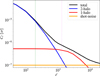Fig. 1. Angular power spectrum of the SKA2 galaxies in z = 0.46 − 0.53, and its different terms. The green dotted vertical line shows the limit of perturbation theory k = 0.15 h Mpc−1 and the violet dotted vertical line indicates the limit of the matryoshka emulator k = 1 h Mpc−1.

Two features are worth noting. First, the one-halo term is roughly constant on multipoles ℓ ≲ 2000, but acquires a significant scale dependence afterwards. From Eq. (11), this scale dependence appears when we hit the radius of the typical host halo mass of the galaxy sample. Second, the high density of galaxies makes shot-noise subdominant, revealing the one-halo term on a wide range of scales. Furthermore, shot-noise can be subtracted exactly, so what is important is its contribution to the covariance, where it contributes to the Gaussian part:

$$\begin{array}{c}\hfill {\mathcal{C}}_{\ell ,{\ell }^{\prime }}^{\mathrm{G}}=\frac{2{(C_{\ell }^{\mathrm{clust}}(i_z)+C_{\ell }^{\mathrm{shot}}(i_z))}^2}{2\ell +1}{\delta }_{\ell ,{\ell }^{\prime }}{\delta }_{i_z,j_z}.\end{array}$$(13)

With this, I find that all multipoles of the power spectrum of SKA2 galaxies can be measured with (S/N)_G > 5 on the whole range ℓ ∈ [2, 20 000] for all redshift bins. Even higher significance is reached for the Euclid photometric sample, which contains more galaxies. This shows that a huge statistical power will be present in the strongly non-linear regime, where the one-halo dominates, both for SKA2 and Euclid.

However, the Gaussian formula does not capture the full covariance, especially on small scales. In this article, I follow the equations for the non-Gaussian part of the covariance from Lacasa (2018), and the numerical approximation and implementation of Lacasa (2020). For the article to be self-contained, I summarise the involved terms. The non-Gaussian covariance is composed of different contributions: super-sample covariance (SSC), braiding covariance, one-halo term, two-halo 1+3 term, three-halo base-0 term, and four-halo third-order term.

$$\begin{array}{c}\hfill {\mathcal{C}}_{\ell ,{\ell }^{\prime }}^{\mathrm{NG}}={\mathcal{C}}_{\ell ,{\ell }^{\prime }}^{\mathrm{SSC}}+{\mathcal{C}}_{\ell ,{\ell }^{\prime }}^{\mathrm{Braid}}+{\mathcal{C}}_{\ell ,{\ell }^{\prime }}^{1\mathrm{h}}+{\mathcal{C}}_{\ell ,{\ell }^{\prime }}^{2\mathrm{h}1+3}+{\mathcal{C}}_{\ell ,{\ell }^{\prime }}^{3\mathrm{hbase}0}+{\mathcal{C}}_{\ell ,{\ell }^{\prime }}^{4\mathrm{h}3}.\end{array}$$(14)

The super-sample covariance is given by

$$\begin{array}{c}\hfill {\mathcal{C}}_{\ell ,{\ell }^{\prime }}^{\mathrm{SSC}}={\displaystyle \int }\mathrm{d}{V}_{\mathit{ab}}{\mathrm{\Psi }}_{\ell }^{\mathrm{sqz}}(z_a){\mathrm{\Psi }}_{{\ell }^{\prime }}^{\mathrm{sqz}}(z_b){\sigma }^2(z_a,z_b)/N_{\mathrm{gal}}{(i_z)}^2{N}_{\mathrm{gal}}{(j_z)}^2,\end{array}$$

where z_a ∈ i_z, z_b ∈ j_z,

$$\begin{array}{c}\hfill {\sigma }^2(z_a,z_b)=\frac{C_{\ell =0}^m(z_a,z_b)}{4\pi }=\frac{1}{2{\pi }^2}{\displaystyle \int }{k}^2\mathrm{d}kP(k|z_{\mathit{ab}})j_0(k{r}_a)j_0(k{r}_b)\end{array}$$(15)

is the SSC kernel, and

$$\begin{array}{c}\hfill {\mathrm{\Psi }}_{\ell }^{\mathrm{sqz}}(z)=4I_1^{{\mathrm{\Sigma }}_2}(k_{\ell }|z)I_1^1(k_{\ell }|z)P(k_{\ell }|z)+I_2^1(k_{\ell },k_{\ell }|z),\end{array}$$(16)

where

$$\begin{array}{c}\hfill I_{\mu }^{{\mathrm{\Sigma }}_2}=\frac{17}{21}{I}_{\mu }^1+\frac{1}{2!}{I}_{\mu }^2\end{array}$$(17)

is the sum of contributions from second-order perturbation theory and second-order bias.

For Braiding covariance, I use the Bij approximation from Lacasa (2020):

$$\begin{array}{c}\hfill {\mathcal{C}}_{\ell ,{\ell }^{\prime }}^{\mathrm{Braid}}=2{\mathrm{\Psi }}_{\ell ,{\ell }^{\prime }}^{\mathrm{alt},\mathrm{int}}(i_z){\mathrm{\Psi }}_{\ell ,{\ell }^{\prime }}^{\mathrm{alt},\mathrm{int}}(j_z)B_{\ell ,{\ell }^{\prime }}(i_z,j_z)\end{array}$$(18)

where

$$\begin{array}{c}\hfill {\mathrm{\Psi }}_{\ell ,{\ell }^{\prime }}^{\mathrm{alt},\mathrm{int}}(i_z)={\displaystyle \int }\mathrm{d}V{\mathrm{\Psi }}_{\ell ,{\ell }^{\prime }}^{\mathrm{alt}}(z)\end{array}$$(19)

and

$$\begin{array}{c}\hfill B_{\ell ,{\ell }^{\prime }}(i_z,j_z)={\displaystyle \sum _{{\ell }_a}}\frac{2{\ell }_a+1}{4\pi }{\left(\begin{array}{ccc}\ell & {\ell }^{\prime }& {\ell }_a\\ 0& 0& 0\end{array}\right)}^2{C}_{{\ell }_a}^{n_g^2}(i_z,j_z),\end{array}$$

with

$$\begin{array}{c}\hfill C_{\ell }^{n_g^2}(i_z,j_z)={\displaystyle \int }\mathrm{d}{V}_{\mathit{ab}}{\overline{n}}_{\mathrm{gal}}{(z_a)}^2{\overline{n}}_{\mathrm{gal}}{(z_b)}^2{C}_{\ell }^m(i_z,j_z)/\left(I^{n_g^2}(i_z)I^{n_g^2}(j_z)\right)\end{array}$$(20)

and

$$\begin{array}{c}\hfill I^{n_g^2}(i_z)={\displaystyle {\int }_{z\in i_z}\mathrm{d}V{\overline{n}}_{\mathrm{gal}}{(z)}^2.}\end{array}$$(21)

Then comes the one-halo term,

$$\begin{array}{c}\hfill {\mathcal{C}}_{\ell ,{\ell }^{\prime }}^{1\mathrm{h}}=\frac{{\delta }_{i_z,j_z}}{4\pi }{\displaystyle \int }\mathrm{d}V{I}_4^0(k_{\ell },k_{\ell },k_{{\ell }^{\prime }},k_{{\ell }^{\prime }}|z)/N_{\mathrm{gal}}{(i_z)}^4,\end{array}$$(22)

the two-halo 1+3 term,

$$\begin{array}{cc}\hfill {\mathcal{C}}_{\ell ,{\ell }^{\prime }}^{2\mathrm{h}1+3}=\frac{2{\delta }_{i_z,j_z}}{4\pi }& {\displaystyle \int }\mathrm{d}V{I}_1^1(k_{\ell }|z)I_3^1(k_{\ell },k_{{\ell }^{\prime }},k_{{\ell }^{\prime }}|z)P(k_{\ell }|z)/N_{\mathrm{gal}}{(i_z)}^4\hfill \\ \hfill & +(\ell \leftrightarrow {\ell }^{\prime }),\hfill \end{array}$$(23)

the three-halo base term (3h-base),

$$\begin{array}{cc}\hfill {\mathcal{C}}_{\ell ,{\ell }^{\prime }}^{3\mathrm{h}-\mathrm{base}0}& =\frac{{\delta }_{i_z,j_z}}{4\pi }{\displaystyle \int }\mathrm{d}V2{\left(I_1^1(k_{\ell }|z)P(k_{\ell }|z)\right)}^2{I}_2^{{\mathrm{\Sigma }}_2}(k_{{\ell }^{\prime }},k_{{\ell }^{\prime }}|z)/N_{\mathrm{gal}}{(i_z)}^4\hfill \\ \hfill & +(\ell \leftrightarrow {\ell }^{\prime })\hfill \\ \hfill & +\frac{4{\delta }_{i_z,j_z}}{4\pi }{\displaystyle \int }\mathrm{d}V2I_1^1(k_{\ell }|z)I_1^1(k_{{\ell }^{\prime }}|z)I_2^{{\mathrm{\Sigma }}_2}(k_{\ell },k_{{\ell }^{\prime }}|z)\hfill \\ \hfill & \times P(k_{\ell }|z)P(k_{{\ell }^{\prime }}|z)/N_{\mathrm{gal}}{(i_z)}^4,\hfill \end{array}$$(24)

and the four-halo term from third-order contributions (4h−3)

$$\begin{array}{cc}\hfill {\mathcal{C}}_{\ell ,{\ell }^{\prime }}^{4\mathrm{h}-3}=& \frac{2{\delta }_{i_z,j_z}}{4\pi }{\displaystyle \int }\mathrm{d}V3!{\left(I_1^1(k_{\ell },z)\right)}^2{I}_1^1(k_{{\ell }^{\prime }},z)I_1^{{\mathrm{\Sigma }}_3}(k_{{\ell }^{\prime }},z)\hfill \\ \hfill & \times P(k_{\ell }|z)P(k_{\ell }|z)P(k_{{\ell }^{\prime }}|z)/N_{\mathrm{gal}}{(i_z)}^4+(\ell \leftrightarrow {\ell }^{\prime }),\hfill \end{array}$$(25)

where

$$\begin{array}{c}\hfill I_{\mu }^{{\mathrm{\Sigma }}_3}\equiv \frac{1023}{1701}{I}_{\mu }^1+\frac{1}{3!}{I}_{\mu }^3\end{array}$$(26)

is the sum of contributions from third-order perturbation theory and third-order bias.

Figure 2 shows all these terms in the case of the variance 𝒞_ℓ, ℓ in the median bin of SKA2.

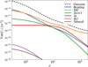Fig. 2. Different contributions to the variance of $C_{\mathcal{l}}^{\text{gal}}$ per individual multipole, for SKA2 galaxies in the median bin z = 0.46 − 0.53.

We see that the 3h-base and 4h-3 terms are negligible for this variance. Indeed, Lacasa (2020) found that they have a negligible impact on the total covariance and on the parameter constraints up to ℓ_max = 2000. Here, I find this result to still hold to ℓ_max = 20 000.

However, Fig. 2 does not sufficiently showcase the complexity and importance of the other non-Gaussian terms, because it only focuses on the diagonal, multipole by multipole. Also, real analyses bin multipoles together, which can significantly change the amplitude of the terms; for instance, the Gaussian variance decreases strongly (typically as 1/Δℓ). Thus, all later results apply the binning of multipoles explained in Sect. 2.1. Therefore, after binning, for the four most important non-Gaussian terms, Fig. 3 shows the correlation matrix ${\mathcal{C}}_{\ell ,{\ell }^{\prime }}/\sqrt{{\mathcal{C}}_{\ell ,\ell }\times {\mathcal{C}}_{{\ell }^{\prime },{\ell }^{\prime }}}$, where each term is normalised by its own diagonal in order to reveal its specific structure.

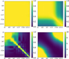Fig. 3. Correlation matrices for the different non-Gaussian covariance terms normalised by their own diagonal for SKA2 galaxies in z = 0.46 − 0.53. From left to right and top to bottom: SSC, one-halo, Braiding, and two-halo 1+3.

We see results consistent with those of Lacasa (2020) on large scales: SSC and one-halo both yield 100% correlated covariance; Braiding is also strongly correlated albeit lower; and two-halo 1+3 is minimal on the diagonal as it correlates large scales with small scales. On top of this, a new behaviour appears at ℓ ≳ 2000: the one-halo stops being 100% correlated and gets closer to diagonal; the same behaviour is seen for Braiding covariance.

Now, in order to obtain a first estimation of the relevance of these non-Gaussian terms, Fig. 4 shows the total covariance, including both the Gaussian and non-Gaussian contributions.

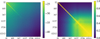Fig. 4. Total covariance matrix, including both Gaussian and non-Gaussian terms, for SKA2 galaxies in z = 0.46 − 0.53. Left: covariance in log colour scale. Right: correlation matrix.

Remembering that the Gaussian covariance only contributes on the diagonal, we see that the non-Gaussian terms become relevant already at multipoles of a few hundred, and at multipoles of a few thousand they dominate the matrix to the point that it becomes > 90% correlated.

3. Fisher constraints

In this section, I use Fisher forecasts to quantify the information content in the galaxy angular power spectrum, and how it varies when extending the range of the multipole of the analysis. I use the covariance matrices shown in the previous section, rescaled with the f_SKY approximation,

$$\begin{array}{c}\hfill {\mathcal{C}}_{\mathrm{partial}-\mathrm{sky}}={\mathcal{C}}_{\mathrm{full}-\mathrm{sky}}/f_{\mathrm{SKY}},\end{array}$$(27)

to account for the partial sky coverage of the surveys. The Fisher information matrix in a given redshift bin then follows:

$$\begin{array}{c}\hfill F_{\alpha ,\beta }(i_z)={\displaystyle \sum _{\ell ,{\ell }^{\prime }={\ell }_{\min }}^{{\ell }_{\max }}{\partial }_{\alpha }{C}_{\ell }^{\mathrm{gal}}(i_z){\mathcal{C}}_{\ell ,{\ell }^{\prime }}^{-1}(i_z,i_z){\partial }_{\beta }{C}_{{\ell }^{\prime }}^{\mathrm{gal}}(i_z),}\end{array}$$(28)

and the matrix summed over all bins is

$$\begin{array}{c}\hfill F_{\alpha ,\beta }={\displaystyle \sum _{i_z,j_z}\sum _{\ell ,{\ell }^{\prime }={\ell }_{\min }}^{{\ell }_{\max }}{\partial }_{\alpha }{C}_{\ell }^{\mathrm{gal}}(i_z){\mathcal{C}}_{\ell ,{\ell }^{\prime }}^{-1}(i_z,j_z){\partial }_{\beta }{C}_{{\ell }^{\prime }}^{\mathrm{gal}}(j_z),}\end{array}$$(29)

where α, β are model parameters, that is, in the following both cosmological parameters (Ω_bh², Ω_ch², H₀, n_S, σ₈, w₀) and HOD parameters $({\alpha }_{\text{sat}},{\sigma }_{\log M},M_{\text{ratio}},M_{\text{min}}^a,M_{\text{min}}^b,M_{\text{min}}^c,M_{\text{min}}^d)$. ${\partial }_{\alpha }{C}_{\ell }^{\mathrm{gal}}$ is the derivative of the power spectrum with respect to the parameter α, and for simplicity I denote multipole bins with their centre throughout the following.

3.1. In angular scales

First, keeping ℓ_min fixed, I study how the Fisher information varies when increasing the maximum multipole of the analysis ℓ_max. For this, I concentrate on the case of the three cosmological parameters that can best be constrained with full shape galaxy power spectra: σ₈, n_S, and w₀. In the case of the median redshift bin of SKA2, Fig. 5 shows the information $F_{\alpha ,\alpha }^{1/2}$ as a function of ℓ_max. This quantity is indeed the inverse of the error bar on the parameter α before marginalisation on other model parameters.

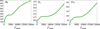Fig. 5. Fisher information $F_{\alpha ,\alpha }^{1/2}$ on σ8, nS, and w0 as a function of the angular cut ℓmax for SKA2 galaxies in z = 0.46 − 0.53.

We see a striking behaviour of the curves: when increasing ℓ_max, the information first rises steadily on linear and weakly non-linear scales, but this increase progressively slows down before coming to a stop around ℓ_max ∼ 2000. A plateau is then present where information has saturated: adding these power spectrum measurements does not bring any (direct) information on cosmological parameters. The extension of this plateau depends on the considered parameter, but for all of them the plateau finally comes to an end and information rises again with a steep slope, a behaviour also seen in Neyrinck & Szapudi (2007). The information brought after the plateau up to ℓ_max = 20 000 is comparable to (for n_S) or larger than (for σ₈ and w₀) the information from linear or weakly non-linear scales before the plateau. This steep rise is the ‘small scale miracle’ that gives this article its title.

Now comes the question of whether this qualitative behaviour is particular to this redshift bin and this survey. Concentrating on the case of dark energy, Fig. 6 shows $F_{w_0,w_0}^{1/2}$ as a function of ℓ_max for different redshift bins of SKA2, both raw (left) and after a rescaling to appreciate the qualitative behaviour of each curve (right). I selected five out of the ten redshift bins to avoid overcrowding the plot, but the omitted bins follow the same qualitative behaviour as the one presented.

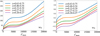Fig. 6. Left: Fisher information on w0, $F_{w_0,w_0}^{1/2}$, as a function of ℓmax for most redshift bins of SKA2, where the bins were selected to maintain the clarity of the plot. Right: same but all curves are rescaled to [0,1] and an offset is added for readability.

We see that all curves follow the qualitative behaviour found previously, with a striking plateau where information saturates before rising again, that is, the small scale miracle. The location (and extent) of the plateau depends on redshift: it slowly moves to smaller angular scales at higher redshifts. I verified that this qualitative behaviour of the information content is also seen in the Euclid survey, the main difference being that the plateau can move to even smaller scales as the sample goes to higher redshift (up to ℓ ∼ 12 000 in the highest bin z = 1.6 − 2.5). I also checked whether or not this qualitative behaviour is seen for other model parameters, and found that it is also clearly present for all the HOD parameters; for the other cosmological parameters Ω_bh² and Ω_ch² (H₀ being almost unconstrained by the galaxy power spectrum) the picture is slightly less clear: a plateau can be seen in some redshift bins but not all; however the rise of information on small scales remains, which is the most important feature. Before interpreting these results, we may wonder what these angular scales of the plateau correspond to in terms of physical scales, and whether or not the redshift evolution of the plateau could be explained by projection onto angles.

3.2. In physical scales

In this section, I want to define a cut-off of the power spectrum data vector in physical scales k_max instead of angular scales ℓ_max. There are two reasons for this: (i) it allows a more natural and redshift-independent understanding of the considered scales and what they correspond to, and (ii) the range of validity of theoretical approaches to non-linearity (perturbation theory, halo model, emulators, etc.) is usually stated in terms of physical scales.

A fixed cut-off in physical scales k_max corresponds to a redshift-dependent cut-off in angular scales ℓ_max(z) = k_max/r(z) with the Limber approximation. That prescription works well for infinitesimal redshift bins and when all multipoles are available. However, in the present case, there is the added complexity that I have predefined redshift and multipole bins. I chose to apply the prescription at the centre of the redshift bin to obtain a first ℓ_max, and then I cut at the multipole bin whose centre is the closest to that ℓ_max.

I defined 16 values of k_max between 0.1 Mpc⁻¹, which is the cut-off of the validity of perturbation theory, and 10 Mpc⁻¹, which is the optimistic cut-off assuming future advances over the current emulators. In the lowest redshift bin, this can correspond to ℓ_max above 20 000, which is why I defined multipole bins up to higher ℓ in Sect. 2.1.

Figure 7 shows the resulting information content $F_{\alpha ,\alpha }^{1/2}$ as a function of k_max for the cosmological parameters σ₈, n_S, and w₀ in the case of the median redshift bin of SKA2.

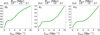Fig. 7. Fisher information on σ8, nS, and w0 as a function of the physical cut kmax for SKA2 galaxies in z = 0.46 − 0.53. The corresponding real-space cut Rmax = 2π/kmax is indicated in the upper x-axis.

We see that the typical behaviour found in Sect. 3.1, with a plateau of information and the small scale miracle, is still present. Furthermore, the plateau happens at a few Mpc⁻¹, which translates in real space to ∼2 Mpc. This is an interesting result as it approximately corresponds to the limit of validity of current emulators.

Now, concentrating on the case of dark energy, Fig. 8 shows the information content on w₀ as a function of k_max for different redshift bins of SKA2.

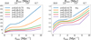Fig. 8. Left: Fisher information on w0 as a function of kmax, for most redshift bins of SKA2. Right: same but all curves are rescaled to [0,1] and an offset is added for readability. The curves are not always perfectly smooth because the translation of kmax into ℓmax is approximate due to binning, as explained in the text.

We see that the location (and extent) of the plateau is redshift dependent, moving to larger physical scales with increasing redshift. This explains why the angular shift of the plateau in Fig. 6 was only weak: with increasing redshift, a fixed physical scale projects onto smaller angular scales, and so both effects (physical mode and projection) go in opposite directions.

3.3. Interpretation

I now give a physical understanding for the presence and location of the plateau of information and the subsequent rise of information on highly non-linear scales. First, we have seen that the plateau appears around ℓ ∼ 2000. Looking at Fig. 1, we see that this is a scale where the one-halo term dominates the power spectrum and is still roughly constant. Looking at Fig. 2 we see that the non-Gaussian covariance is dominated by the SSC and one-halo at this scale. Looking at Fig. 3, we see that these covariance terms are 100% correlated at this scale. Therefore, a first rough statistical picture is that on the scales of the plateau, we are measuring a (roughly) constant power spectrum whose error bars are 100% correlated, and so adding scales does not refine the measurement of that constant, and hence the information content saturates.

From a more physical point of view, the one-halo power spectrum corresponds on large scales to the shot-noise (sometimes called Poisson noise) of the halos. The large-scale value of $C_{\mathcal{l}}^{\text{1h}}$ is a weighted average of the halo number (divided by N_gal(i_z)²), where massive halos have more weight as they host more galaxies. Therefore, in general, on large scales the one-halo power spectrum measures a single parameter: a weighted number of halos in the survey. At ℓ ∼ 2000, we have exhausted the constraining power of this information. Indeed there is a cosmic variance to the number of halos, which is given by the one-halo trispectrum (which quantifies the variance due to the discreteness of halos or Poisson noise) and SSC (which quantifies the variance due to super-survey fluctuations which modulate the number of halos inside the survey). Once this constraining power has been exhausted, as long as $C_{\mathcal{l}}^{\text{1h}}$ remains (roughly) constant, adding scales does not bring anything new. Hence the information content saturates.

Second, we can now understand why this plateau ends and information rises again. The start of this rise depends on the cosmological parameter but is roughly around ℓ ∼ 5000. From Fig. 1, this is a scale where the $C_{\mathcal{l}}^{\text{1h}}$ picks up a significant scale dependence. From Figs. 2 and 3, on these scales the SSC dominates the covariance and is still 100% correlated, while other sources of covariance become closer to diagonal. From a statistical point of view, we are therefore now able to extract information from the scale dependence of the power spectrum, and we are thus recovering constraining power. From a physical point of view, on these smaller scales, $C_{\mathcal{l}}^{\text{1h}}$ stops being dominated by massive (and rare) halos and starts to probe the amount of less massive halos which are smaller; we no longer measure a single parameter and therefore recover constraining power.

Finally, we can refine the picture to understand why the location and extent of the plateau depends on cosmological parameter and redshift. First, for cosmological parameters, the cosmological constraints in the highly non-linear regime come from the fact that by pushing to smaller scales we measure a weighted number of halos with different weights; so we measure the halo mass function (which is sensitive to cosmology), with smaller scales, allowing us to probe smaller masses. The halo mass function is highly sensitive to σ₈ with a steep scaling at high mass, and the exponent of that scaling decreases significantly at lower masses which allows us to quickly break degeneracies. This explains why the plateau of information for σ₈ is the first to end in Fig. 5: as soon as $C_{\mathcal{l}}^{\text{1h}}$ stops being constant, its shape is violently sensitive to σ₈ due to the high scaling; furthermore this scaling is completely different from that of the linear $C_{\mathcal{l}}^{\text{2h}}$ which goes as ${\sigma }_8^2$. By contrast, n_S shows a much longer plateau in Fig. 5; indeed, in order to constrain n_S, we need a high leverage arm in the scales k of the initial power spectrum. The halo mass function is more weakly sensitive to n_S (compared to σ₈), because what enters its prediction is σ(R), the variance of the matter field smoothed at the halo radius scale, which is a convolution of P(k) with a wide kernel. One needs to go to very small masses to probe small k in P(k). This explains why in Fig. 5 the information on n_S starts to rise again only at smaller scales, and why the ratio of information after the plateau to that before is more modest for n_S than σ₈. For the dark energy equation of state, the situation is intermediate between σ₈ and n_S; this is because the halo mass function is sensitive to w₀, though not as much as σ₈, and w₀ also has an influence on the comoving volume dV which enters $C_{\mathcal{l}}^{\text{1h}}$.

Second for the redshift dependence, we see from Fig. 8 that the plateau extends to smaller scales at lower redshifts. This is mostly due to sample selection: because the Euclid and SKA surveys are flux-limited (instead of volume-limited), at lower redshifts we have many more faint galaxies that live in light halos. Therefore, at low z, $C_{\mathcal{l}}^{\text{1h}}$ receives a greater contribution from less massive halos and will therefore pick up a significant scale dependence only on smaller physical scales. This leads the plateau to extend to these smaller physical scales.

3.4. Marginalisation over astrophysics

One issue we need to investigate is whether the cosmological information found at small scales is degenerate or not with the astrophysics. Figure 9 shows the marginalised error bars on σ₈, n_S, and w₀ as a function of k_max for SKA2 galaxies summed over all redshift bins.

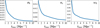Fig. 9. Marginalised error bars on σ8, nS, and w0 as a function of kmax for SKA2 galaxies summed over all redshift bins.

We see that, after marginalising over seven HOD parameters, there is still a substantial improvement of the cosmological errors when increasing k_max. Quantitatively, when pushing k_max from 1 Mpc⁻¹ to 10 Mpc⁻¹, the error bar on σ₈ improves by a factor 9, the error bar on n_S improves by a factor 2.5, and the error bar w₀ improves by a factor 5.2.

In comparison, pushing k_max from 0.1 Mpc⁻¹ to 1 Mpc⁻¹ yields larger improvements, respectively a factor 25 for σ₈, 36 for n_S, and 11 for w₀. Therefore, the astrophysical uncertainties did hamper the improvements of cosmological constraints more in the small scale case (1 → 10 Mpc⁻¹) than in the large scale case (0.1 → 1 Mpc⁻¹). However the resulting improvements still seem worth the effort.

3.5. Potential caveats

Many additional uncertainties in the galaxy modelling could hamper the extraction of cosmological information. It is beyond the scope of this article to study them in detail. It is nonetheless interesting and useful to state them. These uncertainties can be classified in three categories: uncertainties on dark matter halo properties, on the distribution of galaxies inside halos, and on the impact of baryons.

First, properties of dark matter halos may be more complex and uncertain than assumed here. For instance, at the precision of future surveys, it was found that uncertainties in the fitting parameters of the halo mass function should be accounted for (Artis et al. 2021). The halo bias may also not only depend on their mass but on other halo parameters (e.g. age, concentration, spin) as well, an effect called assembly bias (Shi & Sheth 2018; Sato-Polito et al. 2019) that would weaken the extent to which the large-scale galaxy bias is able to constrain HOD parameters. Furthermore, there is uncertainties in the halo shape: scatter should be included in the concentration–mass relation, although this seems to have a negligible impact on the information content (Rizzato et al. 2019), and more generally one should go beyond the usual assumption of spherical halos, for example by accounting for triaxiality (Smith & Watts 2005).

Second, the distribution of galaxies inside halos can be the subject of more uncertainty. More redshift dependence may be allowed for the HOD parameters, notably the high-mass slope α_sat and the ratio M_sat/M_min. The stochastic number of galaxies inside a halo may not follow a Poisson distribution (Cacciato et al. 2013). Furthermore, one should consider that central galaxies have a different spatial distribution from satellites, with the possibility of off-centring for some of them (More et al. 2015). Generally, galaxies could be allowed to follow a profile different from the dark matter NFW profile, though current studies indicate this is not necessary (Bose et al. 2019).

Third, the impact of baryonic physics – and the uncertainties this generates – is currently a hot topic. It has long been known that baryons significantly impact the matter power spectrum on small scales (Jing et al. 2006; Levine & Gnedin 2006), leading to changes of order 10%−30% on the scales relevant to this article (van Daalen et al. 2011), but baryons also impact the halo properties: the halo mass function (Cui et al. 2012), the distribution of subhalos (Romano-Díaz et al. 2010), and halo profiles (Abadi et al. 2010; Duffy et al. 2010). Finally, they also impact the HOD of hosted galaxies (Bose et al. 2019; Beltz-Mohrmann et al. 2020), and the spatial distribution of galaxies inside halos (van Daalen et al. 2014).

The impact of a restricted number of these additional uncertainties is studied in Appendix A, with an extended model that allows for more redshift dependence of the HOD, deviation of the Poisson law for the galaxy distribution, and more freedom in their spatial distribution. This is not meant to be an exhaustive analysis. It shows that the cosmological constraints are indeed degraded, though the degradation is under reasonable control on small scales. At scales k_max ≲ 1 − 2 Mpc⁻¹, the current priors on these additional parameters are nearly enough to mitigate their introduction. On smaller scales, these parameters only degrade constraints on n_S, and better priors would be helpful.

4. Estimating the information in higher orders

Until now, I have focussed the study on the information contained solely in the power spectrum. A first question that arises is whether the qualitative behaviour that I find, that is, the plateau and the small scale miracle, can be expected for higher order statistics. Indeed, future surveys do plan to use this information, for instance at third order with the bispectrum.

From analytical arguments, I indeed expect a similar behaviour for higher order correlation functions and polyspectra. Indeed, these polyspectra also get dominated by a one-halo term in the highly non-linear regime. This one-halo polyspectrum will also be constant on large scales and pick up a scale dependence at the radius corresponding to the typical host halo mass. Therefore, before that scale, the 1h information will be a constant equal to a weighted number of halos in the survey (with weights different from the power spectrum, preferring even more massive halos), and that constant will have a cosmic variance due to SSC and 1h covariance which will limit its constraining power.

A second question that arises is how much constraining power these higher orders can bring on top of the power spectrum. In other words, what is the fundamental limit to the constraining power of the galaxy density field, if we knew how to analyse it optimally? If the galaxy density field were Gaussian, the power spectrum would be the optimal statistic, so the limit would be given by the Fisher information in the power spectrum with a Gaussian covariance. However, the non-linearity introduces another fundamental limit: SSC. Indeed, SSC comes from super-survey modes which change the matter density in the survey by an amount δ_b called the background shift. Wagner et al. (2015) has shown that a portion of the Universe with this background shift evolves identically to a portion of the Universe with a different cosmology. This is the basis of the so-called separate universe approach. Observationally, this means that all cosmological observables, and in particular all statistics of the galaxy density field, will behave as in this different cosmology. Super-sample covariance thus sets a fundamental limit to the cosmological constraints achievable from a given survey volume, independently of the statistics used. Figure 10 compares the Fisher information with the Gaussian+SSC covariance on one hand and the total power spectrum covariance on the other hand, in the case of constraints on σ₈, n_S, and w₀ summed over all redshift bins of SKA2.

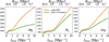Fig. 10. Fisher information on σ8, nS, and w0 as a function of the physical cut kmax, for SKA2 galaxies summed over all redshift bins. The green lower curve shows the power spectrum information with the total covariance, while the orange upper curve uses only the Gaussian + SSC as an estimate of the fundamental limit of the information in the galaxy density field.

We see that there is indeed significant information that can be gained beyond the power spectrum, and that this gain rises rapidly when pushing to smaller scales. To be more quantitative, Table 1 gives the increase of information on σ₈, n_S, and w₀ for some scale cuts.

The gain is the most spectacular for σ₈, more modest but still interesting for n_S, and important for w₀. This can be understood because σ₈ highly influences the amount of non-linearity and therefore high-order statistics allow excellent constraints by breaking degeneracies; for instance, on perturbative scales, the power spectrum scales as (bσ₈)² while the bispectrum scales as $b^3{\sigma }_8^4$, where b is the galaxy bias. For n_S, as argued in Sect. 3.3, constraints in the highly non-linear regime come from probing low-mass halos; however, high-order statistics preferentially probe extreme events, such as massive halos, and so the improvement they bring is more modest. Finally, for w₀ the situation is intermediate between n_S and σ₈ because it impacts the mass function at all masses, and because it also gets constrained by the comoving volume dV whose constraints are improved by high orders. Indeed, for the numerator of the power spectrum (i.e. without the 1/N_gal(i_z)² normalisation), the two-halo term scales as dV² while the one-halo scales as dV; correspondingly, the bispectrum has terms in dV³, dV², and dV. Therefore, high-order statistics allow better constraint of the comoving volume by breaking degeneracies.

5. Discussion

The galaxy angular power spectrum contains valuable raw information on cosmological parameters in the highly non-linear regime dominated by the one-halo term. The main finding of this article is that, in this regime, the information rises steeply with a slope comparable to that in the linear regime. This could in principle yield huge improvement to constraints on the dark energy equation of state.

One condition that needs to be met in order to achieve this improvement is to reach the ‘small scale miracle’ which lies on scales k > 3 Mpc⁻¹. This is currently beyond the reach of the best methods to predict the galaxy power spectrum such as the matryoshka emulator (Donald-McCann et al. 2022), at least at the 1% precision level. However, one can hope to reach these scales in future as the needed improvement is less than a factor 10; there is for instance a proposal that could reach these scales put forward by Hannestad & Wong (2020).

Nevertheless, predicting matter statistics is not a sufficient condition to realise the small scale miracle. To my knowledge, only galaxy and intensity mapping can measure this regime accurately, as cosmic shear, for example, gets dominated by shape noise earlier on. Therefore, we further need a modelling of galaxies to these scales. The most promising prediction framework for this seems to be the halo model. There are issues often raised against the halo model but recent progress could solve them. For example, the problem with mass conservation and large scales is solved in the extended halo model (EHM) of Schmidt (2016); the problem of imprecision in the transition regime between two-halo and one-halo can be solved by the amended halo model (AHM) of Chen & Afshordi (2020). Furthermore, none of these issues affect the small scale miracle, which lies in the highly non-linear regime where the one-halo term is dominant.

Another condition is to control the uncertainties associated with the impact of galaxy formation and baryonic physics. The impact of these uncertainties is partially studied in Sects. 3.4 and 3.5 and Appendix A. Nevertheless, a full assessment is beyond the scope of this article. There is arguably uncertainty as to whether or not we can control these uncertainties. These studies are therefore left for future works.

On a positive note, although using the one-halo term for cosmology is not (yet) the norm in galaxy surveys, this has been done routinely in other surveys. For example, in the case of analyses of the thermal Sunyaev-Zel’dovich (tSZ) effect, the angular power spectrum is entirely dominated by the one-halo term on all scales that have been observed to date. Also, cosmological constraints have been extracted from the tSZ power spectrum for instance by Planck Collaboration XXI (2014), Planck Collaboration XXII (2016). It has been shown that there is high interest in analysing higher order statistics: for example, in Planck Collaboration XXI (2014) the tSZ bispectrum gave cosmological constraints of comparable power to those of the power spectrum, both analyses being limited by uncertainties in the astrophysics of the cluster gas. Furthermore, Hurier & Lacasa (2017) showed that the tSZ bispectrum, power spectrum, and cluster counts have great synergy that breaks degeneracies between cosmological and astrophysical parameters.

Furthermore, in the case of galaxy surveys, Lacasa (2020) studied the galaxy angular power spectrum and showed that the inclusion of non-Gaussian covariance terms in the covariance decreases the degeneracies between cosmological and HOD parameters. Lacasa & Rosenfeld (2016) also showed that the inclusion of cluster counts allows some of these degeneracies to be broken. Therefore, disentangling these two pieces of information could be possible in the one-halo-dominated regime.

In conclusion, there is high interest in pushing the analyses of galaxy clustering to scales of a few Mpc⁻¹ to 10 Mpc⁻¹ dominated by the one-halo term, especially considering that this regime will be measured ‘for free’ with future high-resolution surveys of the large-scale structure of the Universe.

Acknowledgments

Part of this work was supported by funds of the Département de Physique Théorique, Université de Genève. Part of this work was supported by a postdoctoral grant from Centre National d’Études Spatiales (CNES). Part of this work was performed in the context of a visitor grant from the Swiss National Science Foundation, with award number IZSEZ0 207059. I thank the referee for discussion and detailed suggestions that improved this article. Some of the computations made use of the CLASS code (Blas et al. 2011).

References

Appendix A: Extended astrophysical model and impact on the cosmological information content

In this Appendix, I present a study of a +4-parameter extension of the astrophysical base model in order to gauge whether it impacts the extractable cosmological information after marginalisation.

A.1. Extended model: presentation

I first introduce two new parameters to give more freedom to the HOD. The first parameter is called α₁ and it allows for redshift dependence of the high-mass slope of the HOD:

$$\begin{array}{c}\hfill \mathbb{E}[N_{\mathrm{sat}}|N_{\mathrm{cen}}=1]={\left(\frac{M}{M_{\mathrm{sat}}}\right)}^{{\alpha }_{\mathrm{sat}}+{\alpha }_1(1+z)}.\end{array}$$(A.1)

The fiducial value is α₁ = 0, i.e. backward compatibility with the base model.

The second parameter is called β_ratio and it allows for redshift dependence of the central-satellite transition of the HOD:

$$\begin{array}{c}\hfill M_{\mathrm{sat}}=M_{\min }\times M_{\mathrm{ratio}}{(1+z)}^{{\beta }_{\mathrm{ratio}}}.\end{array}$$(A.2)

The fiducial value is β_ratio = 0, i.e. compatible with the base model.

That makes a total of nine HOD parameters in this extended model; it therefore allows nearly as much freedom in the galaxy bias as leaving it as a free parameter in each of the ten redshift bins. The HOD parameters also allow more freedom in the one-halo term of the power spectrum.

The next parameter relates to the stochastic distribution of the number of galaxies in a halo. In the base model used in the main text, this was assumed to follow a Poisson distribution, as supported by simulations (Kravtsov et al. 2004) and observations (Yang et al. 2008). In this extended model, we allow the moments of this distribution to deviate from the Poisson prediction by a deviation parameter 𝒜_P (Cacciato et al. 2013):

$$\begin{array}{c}\hfill ⟨N_{\mathrm{sat}}(N_{\mathrm{sat}}-1)⟩={⟨N_{\mathrm{sat}}⟩}^2\times {\mathcal{A}}_P\end{array}$$(A.3)

so that

$$\begin{array}{c}\hfill ⟨N_{\mathrm{gal}}(N_{\mathrm{gal}}-1)⟩=2⟨N_{\mathrm{sat}}⟩+{⟨N_{\mathrm{sat}}⟩}^2\times {\mathcal{A}}_P.\end{array}$$(A.4)

The fiducial value is 𝒜_P = 1, again compatible with the base model. Following Cacciato et al. (2013), a Gaussian 10% prior can be imposed on this parameter.

𝒜_P exclusively impacts the one-halo term of the power spectrum, thus degrading constraints from it. Effectively, it gives more freedom in how $C_{\mathcal{l}}^{1h}$ probes the halo mass function.

The last parameter relates to the (average) spatial distribution of galaxies inside the halo. We follow the general idea of More et al. (2015) to allow this distribution to deviate from the dark matter distribution, but instead of doing it only for a fraction of central galaxies, we allow it for all galaxies. This is both simpler and more conservative. The parameter is called R_S and rescales the NFW profile:

$$\begin{array}{c}\hfill u_{\mathrm{gal}}(k|M,z)=u_{\mathrm{NFW}}(k\times R_S|M,z).\end{array}$$(A.5)

The fiducial value is R_S = 1 (for compatibility with the base model). We investigate the impact of a Gaussian 20% prior on this parameter.

R_S affects all halo model integrals of the form Eq. 8, allowing more freedom in their scale dependence. In principle, this affects both the two-halo and one-halo term of the power spectrum. Indeed, the one-halo term is directly such an integral, and the two-halo term contains the galaxy bias which is such an integral. However, realistically, R_S will only affect (=degrade) the constraining power from the one-halo term. Indeed, the introduced freedom will be relevant only on halo scales, where the one-halo term has overtaken the two-halo term.

In a way, the 𝒜_P and R_S parameters can be argued to mimic the impact of baryonic physics, because they impact the amplitude and scale dependence of the one-halo term by changing how many (pairs of) galaxies are present in a halo and where they are distributed.

In summary, the extended model is fairly conservative, as it allows more freedom in the galaxy bias, and more importantly much more freedom in the amplitude and scale dependence of the one-halo term.

A.2. Impact on cosmological errors

Figure A.1 shows the marginalised error bars on σ₈, n_S, and w₀ as in Fig. 9 but comparing the base model and the extended model. We note that, here, no prior is imposed at all on any of the additional parameters, and so this is an extremely conservative case.

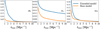Fig. A.1. Marginalised error bars on σ8, nS, and w0 as a function of kmax, depending on the astrophysical model. Blue curve: With the extended model, without any prior on the additional parameter. Orange curve: With the base model of the main text.

Generally, the constraints are vastly weakened at low k_max (I verified that this is even more the case on larger scales: k = 0.1 − 1 Mpc⁻¹), especially for σ₈ which can degrade by up to a factor 8. For n_S, the impact persists to high k_max, though we still get ∼1% constraints, which is fairly good. However, for σ₈ and w₀, the impact seems to decrease largely as we increase k_max.

This last point is not the most clearly visible, as at high k_max the curves are close but also have small values. Furthermore, we would like to see more details on which parameter(s) drive this increase of error bars. This is why Fig. A.2 shows the ratio of the errors to those of the base model, for different extensions.

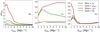Fig. A.2. Ratio of the marginalised error bars from a given model to those of the base model (ref). Considered models: (blue) Base model + α1, (orange), Base model + α1 + βratio, (green) Base model + α1 + βratio + 𝒜P, and (red) Base model + α1 + βratio + 𝒜P + RS = extended model.

With four parameters to set on or off, there should be 2⁴ curves to be exhaustive. But for simplicity and to avoid overcrowding the plot, only four models were chosen: extending the base model by one parameter at a time in the order they are presented in Sect. A.1. One sees that R_S is generally the parameter that degrades the error bars the most. Exceptions are n_S at k_max < 2 Mpc⁻¹ where 𝒜_P has the most significant impact, and w₀ at k_max > 2 Mpc⁻¹ where α₁ has the most significant impact. The figure also confirms the high k_max behaviour hinted at in Fig. 9: when pushing to small scales, the impact of the additional parameters becomes less relevant for σ₈ and w₀. For example, at k_max = 10 Mpc⁻¹, the increase in the error bar is only of 24% for σ₈ and 9% for w₀. For n_S, the impact is more consequent and does not decrease with k_max; it reaches 75% at k_max = 10 Mpc⁻¹. Still, the resulting constraints are comparable to the original ones and are fairly good. One could hope to further improve them by setting priors on the additional parameters.

A.3. Effect of realistic priors

The previous subsection is extremely conservative in not setting any prior on the additional parameter. However, we can realistically set a Gaussian prior of width 10% on 𝒜_P and 20% on R_S. Furthermore, the whole article assumes H₀ to be a free parameter, which degrades the cosmological constraints because galaxy clustering alone has extremely poor constraints on H₀. In reality, one would take a prior on H₀ from CMB or supernovae data². Therefore, I also consider the case for a prior on H₀, of width given by the Planck 2018 constraints (Planck Collaboration VI 2020).

Let us first focus on the astrophysical priors. Figure A.3 shows the impact of the priors on 𝒜_P and R_S on the cosmological errors compared to the base model.

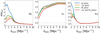Fig. A.3. Ratio of the marginalised error bars to those of the base model (ref), when imposing different realistic priors.

These realistic priors provide a very large improvement of the error on σ₈ at low k_max, dividing the error by up to a factor 3.5 at k_max ∼ 1 Mpc⁻¹. As k_max increases, the impact of the priors lessens, becoming almost insignificant at k_max > 4 Mpc⁻¹. This is however a regime where the errors gradually converge to that of the base model. The results are qualitatively similar for w₀, with the impact of priors saturating even more quickly and the error being already close to that of the base model. The results for n_S are disappointing however: the impact of the priors is very mild.

Second, I studied the impact of an H₀ prior. To provide a fair comparison, I defined the new reference to be the base model with H₀ prior. I found some impact of the H₀ prior on σ₈ and w₀: this somewhat improves the error bars at low k_max, though the priors on 𝒜_P and R_S have a much higher effect there. For n_S, the situation is more interesting: the H₀ prior improves the error ratio significantly and stops it from increasing with k_max. For instance, the quotient of the error in the extended model by that in the base model (both with the H₀ prior) reaches ∼40% at k_max = 10 Mpc⁻¹.

In conclusion, for σ₈ and w₀, the priors on 𝒜_P and R_S are the most needed; they do help a lot where the extended model suffers the most in comparison with the base model (low k_max). For n_S however, it is the H₀ prior that is the most needed; it does help to stabilise the quotient of the error in the extended model by that in the base model, though there is some room for improvement.

A.4. Changing the prior size

Here we ask whether or not having better priors can help to improve our constraints.

A.4.1. General formula: impact of a Gaussian prior on Fisher constraints

This section will make use of the Sherman-Morrison formula (Sherman & Morrison 1950; Bartlett 1951), which gives the impact on matrix inversion of a rank 1 update:

$$\begin{array}{c}\hfill {(A+U{V}^T)}^{-1}=A^{-1}-\frac{A^{-1}·U·V^T·A^{-1}}{1+V^T·A^{-1}·U},\end{array}$$(A.6)

where A is a square matrix, U and V are vectors, and T means the transpose.

In Fisher forecasts, applying a Gaussian prior of width σ² on a model parameter with index i₀ is done by simply adding to the original Fisher matrix F a second matrix F^prior such that

$$\begin{array}{c}\hfill F_{i,j}^{\mathrm{prior}}=\frac{1}{{\sigma }^2}{\delta }_{i,i_0}{\delta }_{i_0,j}.\end{array}$$(A.7)

This matrix is of rank 1 and can be written as $F^{\text{prior}}=U_{\text{p}}{U}_{\text{p}}^T$ with

$$\begin{array}{c}\hfill {\left(U_{\mathrm{p}}\right)}_i=\frac{1}{\sigma }{\delta }_{i,i_0}.\end{array}$$(A.8)

Subsequently, noting the new Fisher matrix $\stackrel{\sim }{F}=F+F^{\mathrm{prior}}$, the Sherman-Morrison formula gives

$$\begin{array}{c}\hfill {\stackrel{\sim }{F}}^{-1}=F^{-1}-\frac{F^{-1}·U_{\mathrm{p}}·U_{\mathrm{p}}^T·F^{-1}}{1+U_{\mathrm{p}}^T·F^{-1}·U_{\mathrm{p}}},\end{array}$$(A.9)

which yields

$$\begin{array}{c}\hfill {\stackrel{\sim }{F}}_{i,j}^{-1}=F_{i,j}^{-1}-\frac{F_{i,i_0}^{-1}{F}_{i_0,j}^{-1}}{{\sigma }^2+F_{i_0,i_0}^{-1}},\end{array}$$(A.10)

or written another way,

$$\begin{array}{c}\hfill {\stackrel{\sim }{F}}^{-1}=F^{-1}-\frac{S(i_0)·S{(i_0)}^T}{{\sigma }^2+F_{i_0,i_0}^{-1}},\end{array}$$(A.11)

where S(i₀) is the column vector (slice) of F⁻¹ at position i₀: ${(i_0)}_i=F_{i,i_0}^{-1}$.

The function smoothly interpolates between the model where the parameter with index i₀ is fixed at its fiducial value (σ = 0) and the original model where it is entirely free (σ → ∞). The difference between the two models is:

$$\begin{array}{c}\hfill \mathrm{\Delta }{\stackrel{\sim }{F}}_{i,j}^{-1}=\frac{F_{i,i_0}^{-1}{F}_{i_0,j}^{-1}}{F_{i_0,i_0}^{-1}}·\end{array}$$(A.12)

In terms of constraining power, the midpoint between the two models is reached for $\sigma =\sqrt{F_{i_0,i_0}^{-1}}$. We note that this midpoint position does not depend on the parameter i considered. It happens when the prior has the same width as the data constraint.

One could further generalise the formula above to allow for simultaneous priors on several parameters (even correlated priors) by using the Woodbury matrix identity (Woodbury 1950). Indeed this identity gives the impact on matrix inversion of an update with arbitrary rank. We refrain from exploring these complications here and will only study one prior at a time in the following subsection.

A.4.2. Application

A first question we need to ask is when can prior help. This is partially answered by Fig. A.3, but one may be concerned that the figure does not show the full potential of priors. Therefore, Fig. A.4 shows the same error bar ratios but now imposing the best possible priors (i.e. σ = 0 in Eq. A.10) on 𝒜_P and R_S. The impact of prior on H₀ is also shown for curiosity.

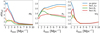Fig. A.4. Ratio of the marginalised error bars to those of the base model (ref), when imposing perfect priors on different parameters.

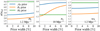Fig. A.5. Ratio of the marginalised error bars to those of the base model (ref), depending on the prior width. kmax is fixed for each parameter to a regime where the priors matter: σ8 and w0 are at a low kmax, while nS is at a high kmax. Current knowledge on H0 is already largely enough to saturate the prior impact, hence the H0 curves are flat. For 𝒜P and RS, the current knowledge is informative enough for σ8 and w0, but better precision at the < 5% level would be nice for futuristic constraints on nS.

As in Fig. A.3, we see that for σ₈ and w₀, these priors are most interesting at low k_max; on smaller scales they become unimportant. However, for n_S, we see that the priors are the most interesting at high k_max, in particular for R_S (and H₀).

In these conditions, the ultimate question is: what prior size would we need to feel these improvements? The main tool to answer this question is based on the remark at the end of Sect. A.4.1: the midpoint is reached when $\sigma =\sqrt{F_{i_0,i_0}^{-1}}$, i.e. when the prior size is equal to the data constraint.

For H₀ the question is then readily answered: the current precision is already sufficient on all scales. Indeed, we have currently 1% precision on H₀, and the constraint from galaxy clustering is severely weaker (500% at best). So we are in the regime $\sigma \ll \sqrt{F_{i_0,i_0}^{-1}}$, and the constraints are saturated to the σ = 0 value (=fixing H₀).

For 𝒜_P and R_S, the answer will depend on the cosmological parameter considered and on scale. First, for σ₈ and w₀, we noted previously that the interesting regime is at low k_max. For instance at k_max = 1.2 Mpc⁻¹ the data constraint on 𝒜_P is 47% and on R_S is 16%. We are therefore in a regime $\sigma <\sqrt{F_{i_0,i_0}^{-1}}$: the current priors are good. Improving these priors would slightly improve cosmological errors, but if it were not possible this would not impair constraints in an irremediable manner. Second, for n_S, we noted previously that the interesting regime is at high k_max. For instance, at k_max = 10 Mpc⁻¹ the data constraint on 𝒜_P is 3.3% and on R_S is 5.6%. We see on Fig. A.4 that prior on 𝒜_P is uninteresting for n_S, so let us concentrate on R_S. Here we are in a regime where the current prior has $\sigma >\sqrt{F_{i_0,i_0}^{-1}}$, i.e. the prior is not sufficient, it fails to improve the constraint on n_S (as can also be seen by comparing Fig. A.3 and Fig. A.4). To mitigate the impact of the model extension, we should aim to have external knowledge to constrain R_S at the < 5% level.

In conclusion, the outlook is optimistic. For near-future analyses staying at low k_max, the current priors on 𝒜_P and R_S are almost sufficient to extract all the constraining power on σ₈ and w₀, and they are not needed for n_S. In a more distant future where analyses can reach high k_max, priors on 𝒜_P and R_S will not be needed for σ₈ and w₀. A < 5% R_S prior will be needed to unlock the full constraining power on n_S, but (i) this would not impair constraints in an irremediable manner, the degradation is at worst 50% (no R_S prior at all, still with a H₀ prior), and (ii) by that time, it is conceivable the community will have improved on current knowledge and reached this precision.

All Tables

All Figures

	Fig. 1. Angular power spectrum of the SKA2 galaxies in z = 0.46 − 0.53, and its different terms. The green dotted vertical line shows the limit of perturbation theory k = 0.15 h Mpc−1 and the violet dotted vertical line indicates the limit of the matryoshka emulator k = 1 h Mpc−1.
In the text

	Fig. 2. Different contributions to the variance of $C_{\mathcal{l}}^{\text{gal}}$ per individual multipole, for SKA2 galaxies in the median bin z = 0.46 − 0.53.
In the text

	Fig. 3. Correlation matrices for the different non-Gaussian covariance terms normalised by their own diagonal for SKA2 galaxies in z = 0.46 − 0.53. From left to right and top to bottom: SSC, one-halo, Braiding, and two-halo 1+3.
In the text

	Fig. 4. Total covariance matrix, including both Gaussian and non-Gaussian terms, for SKA2 galaxies in z = 0.46 − 0.53. Left: covariance in log colour scale. Right: correlation matrix.
In the text

	Fig. 5. Fisher information $F_{\alpha ,\alpha }^{1/2}$ on σ8, nS, and w0 as a function of the angular cut ℓmax for SKA2 galaxies in z = 0.46 − 0.53.
In the text

	Fig. 6. Left: Fisher information on w0, $F_{w_0,w_0}^{1/2}$, as a function of ℓmax for most redshift bins of SKA2, where the bins were selected to maintain the clarity of the plot. Right: same but all curves are rescaled to [0,1] and an offset is added for readability.
In the text

	Fig. 7. Fisher information on σ8, nS, and w0 as a function of the physical cut kmax for SKA2 galaxies in z = 0.46 − 0.53. The corresponding real-space cut Rmax = 2π/kmax is indicated in the upper x-axis.
In the text

	Fig. 8. Left: Fisher information on w0 as a function of kmax, for most redshift bins of SKA2. Right: same but all curves are rescaled to [0,1] and an offset is added for readability. The curves are not always perfectly smooth because the translation of kmax into ℓmax is approximate due to binning, as explained in the text.
In the text

	Fig. 9. Marginalised error bars on σ8, nS, and w0 as a function of kmax for SKA2 galaxies summed over all redshift bins.
In the text

	Fig. 10. Fisher information on σ8, nS, and w0 as a function of the physical cut kmax, for SKA2 galaxies summed over all redshift bins. The green lower curve shows the power spectrum information with the total covariance, while the orange upper curve uses only the Gaussian + SSC as an estimate of the fundamental limit of the information in the galaxy density field.
In the text

	Fig. A.1. Marginalised error bars on σ8, nS, and w0 as a function of kmax, depending on the astrophysical model. Blue curve: With the extended model, without any prior on the additional parameter. Orange curve: With the base model of the main text.
In the text

	Fig. A.2. Ratio of the marginalised error bars from a given model to those of the base model (ref). Considered models: (blue) Base model + α1, (orange), Base model + α1 + βratio, (green) Base model + α1 + βratio + 𝒜P, and (red) Base model + α1 + βratio + 𝒜P + RS = extended model.
In the text

	Fig. A.3. Ratio of the marginalised error bars to those of the base model (ref), when imposing different realistic priors.
In the text

	Fig. A.4. Ratio of the marginalised error bars to those of the base model (ref), when imposing perfect priors on different parameters.
In the text

Fig. A.5. Ratio of the marginalised error bars to those of the base model (ref), depending on the prior width. kmax is fixed for each parameter to a regime where the priors matter: σ8 and w0 are at a low kmax, while nS is at a high kmax. Current knowledge on H0 is already largely enough to saturate the prior impact, hence the H0 curves are flat. For 𝒜P and RS, the current knowledge is informative enough for σ8 and w0, but better precision at the < 5% level would be nice for futuristic constraints on nS.

In the text

References

- Abadi, M. G., Navarro, J. F., Fardal, M., Babul, A., & Steinmetz, M. 2010, MNRAS, 407, 435 [NASA ADS] [CrossRef] [Google Scholar]
- Angulo, R. E., Zennaro, M., Contreras, S., et al. 2021, MNRAS, 507, 5869 [NASA ADS] [CrossRef] [Google Scholar]
- Artis, E., Melin, J.-B., Bartlett, J. G., & Murray, C. 2021, A&A, 649, A47 [NASA ADS] [CrossRef] [EDP Sciences] [Google Scholar]
- Balmès, I., Rasera, Y., Corasaniti, P.-S., & Alimi, J.-M. 2014, MNRAS, 437, 2328 [CrossRef] [Google Scholar]
- Bartlett, M. S. 1951, Ann. Math. Stat., 22, 107 [CrossRef] [Google Scholar]
- Beltz-Mohrmann, G. D., Berlind, A. A., & Szewciw, A. O. 2020, MNRAS, 491, 5771 [NASA ADS] [CrossRef] [Google Scholar]
- Blas, D., Lesgourgues, J., & Tram, T. 2011, JCAP, 2011, 034 [Google Scholar]
- Bose, S., Eisenstein, D. J., Hernquist, L., et al. 2019, MNRAS, 490, 5693 [CrossRef] [Google Scholar]
- Bull, P. 2016, ApJ, 817, 26 [NASA ADS] [CrossRef] [Google Scholar]
- Bullock, J. S., Kolatt, T. S., Sigad, Y., et al. 2001, MNRAS, 321, 559 [Google Scholar]
- Cacciato, M., van den Bosch, F. C., More, S., Mo, H., & Yang, X. 2013, MNRAS, 430, 767 [Google Scholar]
- Cataneo, M., Lombriser, L., Heymans, C., et al. 2019, MNRAS, 488, 2121 [Google Scholar]
- Cataneo, M., Emberson, J. D., Inman, D., Harnois-Déraps, J., & Heymans, C. 2020, MNRAS, 491, 3101 [CrossRef] [Google Scholar]
- Chen, A. Y., & Afshordi, N. 2020, Phys. Rev. D, 101, 103522 [NASA ADS] [CrossRef] [Google Scholar]
- Contigiani, O., Vardanyan, V., & Silvestri, A. 2019, Phys. Rev. D, 99, 064030 [NASA ADS] [CrossRef] [Google Scholar]
- Cooray, A., & Sheth, R. 2002, Phys. Rep., 372, 1 [Google Scholar]
- Cui, W., Borgani, S., Dolag, K., Murante, G., & Tornatore, L. 2012, MNRAS, 423, 2279 [NASA ADS] [CrossRef] [Google Scholar]
- Donald-McCann, J., Beutler, F., Koyama, K., & Karamanis, M. 2022, MNRAS, 511, 3768 [NASA ADS] [CrossRef] [Google Scholar]
- Duffy, A. R., Schaye, J., Kay, S. T., et al. 2010, MNRAS, 405, 2161 [NASA ADS] [Google Scholar]
- Euclid Collaboration (Blanchard, A., et al.) 2020, A&A, 642, A191 [NASA ADS] [CrossRef] [EDP Sciences] [Google Scholar]
- Giblin, B., Cataneo, M., Moews, B., & Heymans, C. 2019, MNRAS, 490, 4826 [Google Scholar]
- Hannestad, S., & Wong, Y. Y. Y. 2020, JCAP, 2020, 028 [CrossRef] [Google Scholar]
- Hoffmann, K., Bel, J., Gaztañaga, E., et al. 2015, MNRAS, 447, 1724 [NASA ADS] [CrossRef] [Google Scholar]
- Hurier, G., & Lacasa, F. 2017, A&A, 604, A71 [NASA ADS] [CrossRef] [EDP Sciences] [Google Scholar]
- Jing, Y. P., Zhang, P., Lin, W. P., Gao, L., & Springel, V. 2006, ApJ, 640, L119 [Google Scholar]
- Knabenhans, M., Stadel, J., Marelli, S., et al. 2019, MNRAS, 484, 5509 [Google Scholar]
- Kobayashi, Y., Nishimichi, T., Takada, M., & Takahashi, R. 2020, Phys. Rev. D, 101, 023510 [NASA ADS] [CrossRef] [Google Scholar]
- Kravtsov, A. V., Berlind, A. A., Wechsler, R. H., et al. 2004, ApJ, 609, 35 [Google Scholar]
- Lacasa, F. 2018, A&A, 615, A1 [NASA ADS] [CrossRef] [EDP Sciences] [Google Scholar]
- Lacasa, F. 2020, A&A, 634, A74 [NASA ADS] [CrossRef] [EDP Sciences] [Google Scholar]
- Lacasa, F., & Rosenfeld, R. 2016, JCAP, 8, 005 [Google Scholar]
- Lange, J. U., van den Bosch, F. C., Zentner, A. R., et al. 2019, MNRAS, 490, 1870 [NASA ADS] [CrossRef] [Google Scholar]
- Laureijs, R., Amiaux, J., Arduini, S., et al. 2011, ArXiv e-prints [arXiv:1110.3193] [Google Scholar]
- Levine, R., & Gnedin, N. Y. 2006, ApJ, 649, L57 [CrossRef] [Google Scholar]
- Lopes, R. C. C., Voivodic, R., Abramo, L. R., & Sodré, L., Jr. 2018, JCAP, 9, 010 [NASA ADS] [CrossRef] [Google Scholar]
- Lopes, R. C. C., Voivodic, R., Abramo, L. R., & Sodré, L., Jr. 2019, JCAP, 7, 026 [CrossRef] [Google Scholar]
- Loureiro, A., Moraes, B., Abdalla, F. B., et al. 2019, MNRAS, 485, 326 [NASA ADS] [CrossRef] [Google Scholar]
- LSST Science Collaboration (Abell, P. A., et al.) 2009, ArXiv e-prints [arXiv:0912.0201] [Google Scholar]
- Maartens, R., Abdalla, F. B., Jarvis, M., & Santos, M. G. 2015, Proceedings, Advancing Astrophysics with the Square Kilometre Array (AASKA14), 016 [CrossRef] [Google Scholar]
- More, S., Miyatake, H., Mandelbaum, R., et al. 2015, ApJ, 806, 2 [CrossRef] [Google Scholar]
- Navarro, J. F., Frenk, C. S., & White, S. D. 1997, ApJ, 490, 493 [NASA ADS] [CrossRef] [Google Scholar]
- Neyrinck, M. C., & Szapudi, I. 2007, MNRAS, 375, L51 [NASA ADS] [CrossRef] [Google Scholar]
- Ntampaka, M., Eisenstein, D. J., Yuan, S., & Garrison, L. H. 2020, ApJ, 889, 151 [NASA ADS] [CrossRef] [Google Scholar]
- Planck Collaboration XXI. 2014, A&A, 571, A21 [NASA ADS] [CrossRef] [EDP Sciences] [Google Scholar]
- Planck Collaboration XXII. 2016, A&A, 594, A22 [NASA ADS] [CrossRef] [EDP Sciences] [Google Scholar]
- Planck Collaboration VI. 2020, A&A, 641, A6 [NASA ADS] [CrossRef] [EDP Sciences] [Google Scholar]
- Rizzato, M., Benabed, K., Bernardeau, F., & Lacasa, F. 2019, MNRAS, 490, 4688 [NASA ADS] [CrossRef] [Google Scholar]
- Romano-Díaz, E., Shlosman, I., Heller, C., & Hoffman, Y. 2010, ApJ, 716, 1095 [CrossRef] [Google Scholar]
- Ryu, S., & Lee, J. 2020, ApJ, 889, 62 [NASA ADS] [CrossRef] [Google Scholar]
- Sato-Polito, G., Montero-Dorta, A. D., Abramo, L. R., Prada, F., & Klypin, A. 2019, MNRAS, 487, 1570 [NASA ADS] [CrossRef] [Google Scholar]
- Schmidt, F. 2016, Phys. Rev. D, 93, 063512 [NASA ADS] [CrossRef] [Google Scholar]
- Sherman, J., & Morrison, W. J. 1950, Ann. Math. Stat., 21, 124 [CrossRef] [Google Scholar]
- Shi, J., & Sheth, R. K. 2018, MNRAS, 473, 2486 [NASA ADS] [CrossRef] [Google Scholar]
- Smith, R. E., & Watts, P. I. R. 2005, MNRAS, 360, 203 [NASA ADS] [CrossRef] [Google Scholar]
- Tansella, V. 2018, Phys. Rev. D, 97, 103520 [Google Scholar]
- Tinker, J., Kravtsov, A. V., Klypin, A., et al. 2008, ApJ, 688, 709 [Google Scholar]
- Tinker, J. L., Robertson, B. E., Kravtsov, A. V., et al. 2010, ApJ, 724, 878 [NASA ADS] [CrossRef] [Google Scholar]
- Tröster, T., Sánchez, A. G., Asgari, M., et al. 2020, A&A, 633, L10 [NASA ADS] [CrossRef] [EDP Sciences] [Google Scholar]
- van Daalen, M. P., Schaye, J., Booth, C. M., & Dalla Vecchia, C. 2011, MNRAS, 415, 3649 [Google Scholar]
- van Daalen, M. P., Schaye, J., McCarthy, I. G., Booth, C. M., & Dalla Vecchia, C. 2014, MNRAS, 440, 2997 [NASA ADS] [CrossRef] [Google Scholar]
- Wagner, C., Schmidt, F., Chiang, C.-T., & Komatsu, E. 2015, MNRAS, 448, L11 [CrossRef] [Google Scholar]
- Woodbury, M. A. 1950, Memorandum Rept. 42, Statistical Research Group [Google Scholar]
- Yang, X., Mo, H. J., & van den Bosch, F. C. 2008, ApJ, 676, 248 [Google Scholar]
- Zehavi, I., Zheng, Z., Weinberg, D. H., et al. 2011, ApJ, 736, 59 [NASA ADS] [CrossRef] [Google Scholar]