| Issue |
A&A
Volume 652, August 2021
|
|
|---|---|---|
| Article Number | A11 | |
| Number of page(s) | 23 | |
| Section | Extragalactic astronomy | |
| DOI | https://doi.org/10.1051/0004-6361/202040232 | |
| Published online | 04 August 2021 | |
COALAS
I. ATCA CO(1–0) survey and luminosity function in the Spiderweb protocluster at z = 2.16
1
Instituto de Astrofísica de Canarias (IAC), 38205 La Laguna, Tenerife, Spain
e-mail: shuowen.jin@gmail.com
2
Universidad de La Laguna, Dpto. Astrofísica, 38206 La Laguna, Tenerife, Spain
3
National Radio Astronomy Observatory, 520 Edgemont Road, Charlottesville, VA 22903, USA
4
INAF – Osservatorio Astronomico di Cagliari, Via della Scienza 5, 09047 Selargius, CA, Italy
5
International Centre for Radio Astronomy Research (ICRAR), M468, University of Western Australia, 35 Stirling Hwy, Crawley, WA 6009, Australia
6
ARC Centre of Excellence for All Sky Astrophysics in 3 Dimensions (ASTRO 3D), Australia
7
Cosmic Dawn Center (DAWN), Copenhagen, Denmark
8
The University of Manchester, Oxford Road, Manchester M13 9PL, UK
9
Astronomy Unit, Department of Physics, University of Trieste, Via Tiepolo 11, 34131 Trieste, Italy
10
INAF – Osservatorio Astronomico di Trieste, Via Tiepolo 11, 34131 Trieste, Italy
11
IFPU – Institute for Fundamental Physics of the Universe, Via Beirut 2, 34014 Trieste, Italy
12
Sorbonne Université, CNRS, UMR 7095, Institut d’Astrophysique de Paris, 98bis Blvd Arago, 75014 Paris, France
13
Sub-dept of Astrophysics, Physics, University of Oxford, Denys Wilkinson Building, Keble Road, Oxford OX1 3RH, UK
14
Department of Astronomy, The University of Texas at Austin, 2515 Speedway Blvd Stop C1400, Austin, TX 78712, USA
15
CSIRO Astronomy and Space Science, PO Box 76, Epping, NSW 1710, Australia
16
Western Sydney University, Locked Bag 1797, Penrith, NSW 2751, Australia
17
International Centre for Radio Astronomy Research, Curtin University, Bentley, WA 6102, Australia
18
Subaru Telescope, National Astronomical Observatory of Japan, National Institutes of Natural Sciences, 650 North A’ohoku Place, Hilo, HI 96720, USA
19
European Southern Observatory, Karl-Schwarzschild-Straße 2, 85748 Garching, Germany
20
School of Physics and Astronomy, University of Nottingham, University Park, Nottingham NG7 2RD, UK
21
Astronomical Institute, Tohoku University, Aoba-ku, Sendai 980-8578, Japan
22
Leiden Observatory, PO Box 9513 2300 RA Leiden, The Netherlands
23
Observatório Nacional, Rua General José Cristino, 77, Sao Cristóvao, Rio de Janeiro, RJ 20921-400, Brazil
24
Instituto de Radioastronomía Milimétrica, Av. Divina Pastora 7, Núcleo Central, 18012 Granada, Spain
25
University Vienna, Department of Astrophysics, Türkenschanzstraße 17, 1180 Wien, Austria
Received:
24
December
2020
Accepted:
15
March
2021
We report a detailed CO(1−0) survey of a galaxy protocluster field at z = 2.16, based on 475 h of observations with the Australia Telescope Compact Array. We constructed a large mosaic of 13 individual pointings, covering an area of 21 arcmin2 and ±6500 km s−1 range in velocity. We obtained a robust sample of 46 CO(1−0) detections spanning z = 2.09 − 2.22, constituting the largest sample of molecular gas measurements in protoclusters to date. The CO emitters show an overdensity at z = 2.12 − 2.21, suggesting a galaxy super-protocluster or a protocluster connected to large-scale filaments of ∼120 cMpc in size. We find that 90% of CO emitters have distances >0.′5−4′ to the center galaxy, indicating that small area surveys would miss the majority of gas reservoirs in similar structures. Half of the CO emitters have velocities larger than escape velocities, which appears gravitationally unbound to the cluster core. These unbound sources are barely found within the R200 radius around the center, which is consistent with a picture in which the cluster core is collapsed while outer regions are still in formation. Compared to other protoclusters, this structure contains a relatively higher number of CO emitters with relatively narrow line widths and high luminosities, indicating galaxy mergers. We used these CO emitters to place the first constraint on the CO luminosity function and molecular gas density in an overdense environment. The amplitude of the CO luminosity function is 1.6 ± 0.5 orders of magnitude higher than that observed for field galaxy samples at z ∼ 2, and one order of magnitude higher than predictions for galaxy protoclusters from semi-analytical SHARK models. We derive a high molecular gas density of 0.6 − 1.3 × 10⁹ M⊙ cMpc−3 for this structure, which is consistent with predictions for cold gas density of massive structures from hydro-dynamical DIANOGA simulations.
Key words: Galaxy: evolution / galaxies: formation / galaxies: clusters: individual: Spiderweb / galaxies: high-redshift / galaxies: ISM / ISM: molecules
© ESO 2021
1. Introduction
Galaxy protoclusters (see Overzier 2016 for a review) are expected to contribute significantly to the star formation rate density (SFRD) at high redshifts (Chiang et al. 2017), for example, 20−50% at z > 2. Thus, understanding how clusters assembled their mass is of critical importance. Molecular gas is the reservoir in which the stars form. Measuring the molecular gas content and distribution in galaxies as a function of environment and epoch is crucial for developing our understanding of how galaxies form and evolve. Moreover, since the potential impact of environment can be large on galaxy evolution as evidenced by the tightness of the color-luminosity sequence in local clusters and the morphology-density relation (Dressler 1980; Davies et al. 2014), constraining the evolution of the gas in galaxy clusters and protoclusters offers us key tests of galaxy evolution models.
As a proxy for the cold molecular gas content, CO surveys of random fields (e.g., Walter et al. 2016; Riechers et al. 2019, 2020a; Decarli et al. 2019, 2020) have revealed the evolution of molecular gas density throughout cosmic history. The ASPECS survey (Walter et al. 2016) conducted the first blind CO search with the Atacama Large Millimeter Array (ALMA) in the Hubble Ultra Deep Field (HUDF). This survey revealed an elevated CO luminosity function at z ∼ 2 with respect to the local Universe and an evolution of cosmic molecular gas density within galaxies as a function of redshift (Decarli et al. 2016). Using the Karl G. Jansky Very Large Array (VLA) observations, the COLDz project (Riechers et al. 2019) provided detailed measurements of the CO luminosity function and molecular gas density at z = 2 − 3 and z = 5 − 7 via CO(1−0) and CO(3−2) detections, respectively. Recently, based on the reported CO detections by González-López et al. (2019) and Aravena et al. (2019), Decarli et al. (2019, 2020) constructed the CO luminosity function out to z ∼ 4 and found that the observed evolution of the molecular gas density tracks the evolution of the cosmic star formation rate density. This finding is confirmed by the PHIBSS2 survey (Lenkić et al. 2020) with CO observations with the Plateau de Bure Interferometer (PdBI). These CO surveys focus on field galaxy samples, however, the molecular gas density in dense environments such as galaxy (proto)clusters has not yet been constrained.
Over the last few years, there have been significant efforts to observe CO in high-redshift (proto)cluster environments (e.g., Emonts et al. 2016, 2018; Hayashi et al. 2017; Noble et al. 2017, 2019; Casey 2016; Wang et al. 2016, 2018; Dannerbauer et al. 2017; Rudnick et al. 2017; Stach et al. 2017; Oteo et al. 2018; Coogan et al. 2018; Miller et al. 2018; Tadaki et al. 2019; Gómez-Guijarro et al. 2019; Lee et al. 2019; Castignani et al. 2019; Hill et al. 2020; Ivison et al. 2020; Spérone-Longin et al. 2021). However, due to the frequency coverage, ALMA line surveys mostly target high-J CO(J, J − 1) transitions (J ≥ 2) that could introduce uncertainties into the total molecular gas mass due to unknown gas excitation (e.g., Dannerbauer et al. 2009; Daddi et al. 2015; Liu et al. 2015; Yajima et al. 2021). The ground-state CO transition (rest-frame 115.27 GHz, J = 1) is extensively used as the best tracer of the total cold molecular gas mass (e.g., Ivison et al. 2011; Emonts et al. 2013). Using deep CO(1−0) observations with the VLA, Rudnick et al. (2017) revealed two gas-rich cluster members at z = 1.62 and found that cluster members have comparable gas fractions and star formation efficiencies (SFEs) with respect to field galaxies, which is consistent with field-scaling relations between the molecular gas content, stellar mass, SFR, and redshift. In the z = 2.5 CL J1001 (proto)cluster field, Wang et al. (2016, 2018) conducted VLA observations of the CO(1−0) transition. They found low gas content and elevated SFEs in cluster members compared to field galaxies, presenting evidence for an environmental impact on the molecular gas reservoirs and SFEs of z = 2 cluster galaxies. However, the abovementioned CO(1−0) observations in high-z galaxy clusters targeted either individual cluster members or the central region of a (proto)cluster core (e.g., Emonts et al. 2016, 2018; Dannerbauer et al. 2017; Wang et al. 2018; Champagne et al. 2021), and thus introduced a bias in their interpretation in the context of galaxy formation and evolution, as protoclusters can be extended up to 30′ on the sky (respectively up to 15 Mpc in physical units; Muldrew et al. 2015; Casey 2016), and superstructure has been found with a comoving size of ∼120 cMpc at z > 2 (Cucciati et al. 2018). Clearly, surveys covering the large volume of a galaxy protocluster in the distant Universe are still missing and would allow us to characterize the CO luminosity function and molecular gas density in such an environment.
To this end, the Spiderweb protocluster field at z = 2.16, being a prominent and well-studied example of a cluster in formation, is an ideal laboratory for such a study (Miley et al. 2006). This protocluster has been continually observed and results in rich, multiwavelength datasets. It hosts a significant overdensity of Lyα emitters (LAEs; Pentericci et al. 2000; Kurk et al. 2000), Hα emitters (HAEs; Kuiper et al. 2011; Koyama et al. 2013; Shimakawa et al. 2014, 2018), extremely red objects (ERO; Kurk et al. 2004), and submillimeter galaxies (SMGs; Rigby et al. 2014; Dannerbauer et al. 2014). A 10-Mpc-scale filament traced by HAEs has been identified across this region (Koyama et al. 2013; Shimakawa et al. 2018). Meanwhile, the SFRD based on far-infrared/submillimeter measurements appears high, ∼1500 M⊙ yr−1 Mpc−3 (Dannerbauer et al. 2014). Recently, massive gas reservoirs in this structure have been revealed via CO(1−0) observations with the Australia Telescope Compact Array (ATCA). Emonts et al. (2016) found a large reservoir of molecular gas extending across 70 kpc around the central starbursting radio galaxy MRC1138−262. This reservoir of molecular gas fuels in situ star formation (Hatch et al. 2008) and drives the growth of a massive central-cluster galaxy, suggesting that the brightest cluster galaxies could form out of extended, recycled gas at high redshift. This work demonstrated the power of ATCA to detect the most extended CO(1−0) emission. Subsequently, Dannerbauer et al. (2017) discovered an extended rotating disk (40 kpc) with a massive molecular gas mass Mmol = 2 × 10¹¹ M⊙ in a normal star-forming galaxy in this protocluster, and found no evidence of environmental impact on the SFE. More recently, one more protocluster galaxy was found in CO(1−0) in the region between the radio galaxy and HAE229 (Emonts et al. 2018). As these CO(1−0) observations target only a small area around the center radio galaxy, the very limited number of detections cannot constrain the CO luminosity function and total gas density in co-moving volume. On the other hand, the physical scale of the protocluster is unknown. This is due to the narrowness of the redshift range probed in narrowband imaging surveys and the rest-frame UV/optical lines of dusty member galaxies can be severely attenuated, making the identification of cluster membership difficult to complete. A large scale CO survey with a broad bandwidth will help us to find additional cluster members that are missed by optical/NIR surveys and could be able to reveal wider structure. Moreover, the SFRD found in Dannerbauer et al. (2014) is well above the predictions of simulations and semi-analytical models (e.g., Bassini et al. 2020; Lim et al. 2021). It is unclear if the molecular gas density compared to the field sample is similarly overdense to the SFRD, and would be of great interest to compare the observed gas density to predictions from cosmological simulations (e.g., Lagos et al. 2020; Bassini et al. 2020). Thus, a dedicated CO(1−0) survey is urgently needed in order to constrain the molecular gas density in this structure and help to clarify these issues.
As part of the present study, we report the first result of the COALAS (CO ATCA Legacy Archive of Star-forming galaxies) project, focusing on the ATCA CO(1−0) observations of the Spiderweb cluster field at z = 2.16. In Sect. 3, we discuss the source extraction and construct the CO-emitter catalog. In Sect. 4, we present the results of the catalog. In addition, we constrain the CO(1−0) luminosity function and molecular gas density of this structure. We close the paper with a discussion in Sect. 5 and present the major conclusions of this study in Sect. 6. We adopted a flat ΛCDM cosmology with H0 = 71 km s−1 Mpc−1, ΩM = 0.27, Λ0 = 0.73 (Spergel et al. 2003, 2007), and a Chabrier IMF (Chabrier 2003).
2. Observations and data reduction
The COALAS project1 is a large program (ID: C3181, PI: H. Dannerbauer) with ATCA. The observations took place from April 2017 to March 2020. A major goal of this project is to study the impact of environment on the cold molecular gas content via the CO(1−0) transition. In total, we obtained 820 h observing time with the ATCA (including compensation for bad weather). The COALAS large program consists of well-covered “field” targets from the Extended Chandra Deep Field-South (ECDFS) and “cluster” targets from the Spiderweb protocluster (z = 2.16). In this work, we only present the results in the Spiderweb protocluster field, while the work in ECDFS will be presented in Thomson et al. (in prep.).
In addition, we included observations of several LABOCA-selected sources (ID: 2014OCTS/C3003 and 2016AOPRS/C3003: PI: H. Dannerbauer, high resolution pointings focusing on DKB01−03 ID: 2017APRS/C3003, PI: B. Emonts), the center radio galaxy, and the HAE229 (Emonts et al. 2016; Dannerbauer et al. 2017). These observations were finished before the large program started and were conducted in the same Spiderweb field at the same frequency as the large program. In total, we observed the Spiderweb protocluster field for 475 h (including bad weather). We stress that ATCA is currently the only facility in the southern hemisphere that can target the lowest CO transition of z ∼ 2 galaxies. The situation will change with the installation of ALMA band 1.
As shown in Fig. 1, including data from Emonts et al. (2016, 2018) and Dannerbauer et al. (2017), 13 pointings have been observed at 36.5 GHz in total (the redshifted CO(1−0) transition) with a 2 GHz bandwidth. The pointings were designed as such in order to maximize the number of known sources (with spectroscopic redshifts from the rest-frame UV/optical) per pointing. Therefore, the spacing between the pointing varies, and the depth of the mosaic is not homogeneous. The pointings primarily cover submillimeter galaxies detected with LABOCA that are most probably physically related to the protocluster (Dannerbauer et al. 2014), secondarily the HAEs confirmed in the same structure (Koyama et al. 2013; Shimakawa et al. 2014). We observed at different configurations for about eight hours per night, mostly using the most compact array configuration, such as H75, H168, or H214 (see details in Table 1), and the beam size varies from 4″ to 14″. Therefore, in principle we do not expect to resolve sources in the data cube. However, because of the very compact array configurations (baselines < 100 m), our ATCA observations are very sensitive to low-surface-brightness emission from extended molecular gas reservoirs, ensuring that we obtain reliable mass estimates. We summarize the observations of the 13 individual pointings in Table 1, in which 11 of them are from the COALAS large program. The data of the pointings of MRC1138 and HAE229 are taken from previous studies of Emonts et al. (2016, 2018) and Dannerbauer et al. (2017). For the remaining 11 pointings, the phases are calibrated every 15 min with a short (∼2 min) scan on a nearby calibrator 1124−186. 1124−186 is also used for bandpass calibration, which calibrated out a uniform sensitivity over the frequency range covered. Flux calibration was done on PKS 1934−638. Following Emonts et al. (2014), a conservative 20% uncertainty in the measured fluxes is assumed to account for the uncertainty in absolute flux calibration. However, this does not affect the source extraction via signal-to-noise ratio (S/N) in the data cube (see Sect. 3).
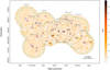 |
Fig. 1. S/N map of line candidates (Sect. 3.1) in the ATCA mosaic. The S/N is the maximum S/N computed in the 1D spectrum on each pixel by our algorithm MaxFinder (see details in Sect. 3.1). The color bar values are limited in 1.5 < S/N < 6.5 for fair visibility of detections. ATCA pointings are shown in gray circles with a radius of 0.9′. Gray solid circles mark the pointings MRC1138 in Emonts et al. (2016) and HAE229 in Dannerbauer et al. (2017), respectively. The cyan contour encloses the area with rms < 1 mJy beam−1. Detected sources are marked by solid the following solid color circles: blue: category A; magenta: category B; green: category C (see details in Sect. 3.3). |
Overview of observations.
We used the software packages MIRIAD (Sault et al. 1995) and Karma (Gooch 1996) for the data reduction and visualization, following the strategy described in detail in Emonts et al. (2014, 2016) and Dannerbauer et al. (2017). We imaged the ATCA data cube with natural weighting using the task INVERT for each individual pointing. The full width half maximum (FWHM) of the ATCA primary beam is 70″ at 7 mm. We imaged each individual pointing with a radius of 0.9′ so that adjacent pointings significantly overlap. The total sky coverage of the 13 ATCA pointings is 25.8 arcmin2, while sources are only detected in regions with rms noise < 1 mJy per beam which corresponds to an area of 21.3 arcmin2. The data cubes were imaged using pixel size of 1.5″ and channel width of 40 km s−1. We applied a Hanning smooth, resulting in a resolution of 80 km s−1. The continuum was separated from the line by fitting a straight line to the line-free channels in the uv domain. Velocities are in the optical frame relative to z = 2.1612, spanning ±7000 km s−1.
We linearly combined the 13 pointings using the task LINMOS after correcting for primary beam attenuation. The rms level of individual pointing are 0.13 − 0.29 mJy per beam (in 40 km s−1 channel) on the phase center of each pointing as listed in Table 1, while the S/N in the overlapping regions improved, with an rms of 0.1 − 1 mJy over the whole field after primary beam correction. The deepest area has an rms of 0.09 mJy per beam and is centered on the radio galaxy MRC1138−262 and HAE229, which are covered by 3 − 4 individual pointings. Because none of the new CO signals in our survey is strong enough to have significant sidelobes, we did not deconvolve our images, and we therefore performed our analysis on the “dirty” cube, following the previous studies in Emonts et al. (2016, 2018) and Dannerbauer et al. (2017).
3. Line search
We adopted two major methods to search for CO lines in the ATCA data cube: (i) our code, MaxFinder, which is an algorithm searching for the maximum S/N of candidate lines on each pixel and matching counterparts in optical images (Sect. 3.1); and (ii) the Source Finding Application (SoFiA), which is a blind source finding pipeline intended to find and parameterize lines in data cubes (Serra et al. 2015), see details in Sect. 3.2. As a complementary approach, we searched for CO lines using the reshifts of the HAEs in this field. We summarize the selection of the final catalog in Sect. 3.3. The statistical properties of the catalog (e.g., completeness and flux boosting) are described in Sect. 3.4.
3.1. MaxFinder
The MaxFinder code is inspired by previous work on manual extraction of CO(1−0) emission from ATCA cubes (Emonts et al. 2014, 2016, 2018; Dannerbauer et al. 2017). Equivalently, the MaxFinder source extraction code will search for the most probable line candidate on every position (i.e., pixel) and look for their optical or near-infrared (NIR) counterparts afterwards. We ran the MaxFinder on the large mosaic made of all 13 pointings. This large mosaic contains the best S/N in regions overlapped by multiple pointings, albeit with variations in resolution, enabling us to search for the most probable line candidates in the data cube. First, MaxFinder extracts the spectrum on each pixel and calculates the weighted average over any two channels. Given that the sensitivity is uniform over the full ATCA spectral range, the flux uncertainty is defined as the standard deviation of the full spectrum without Hanning smoothing. We compute the weighted average over each two arbitrary channels, and select the two channels ni and nj that maximize the weighted average. Second, we define the range of line as channels lying in the full width at zero intensity (FWZI) that contains the channels ni and nj. The MaxFinder determines the FWZI range by searching for the first negative channel on the left (right) side of channel ni (nj). Adopting Eq. (2) in Emonts et al. (2014), the line flux is integrated over the FWZI range, and uncertainty of the line flux is calculated as  . Thus, the S/N is
where σ is the rms noise, Δv is the channel width and FWZI the range over which the line flux was integrated. This way, we keep the calculations consistent with previous work by our team. Then we calculate signal and noise of the candidate line on each pixel and make a large S/N mosaic, as shown in Fig. 1. We note that the radio galaxy MRC1138−262 (Emonts et al. 2013, 2016) and the HAE229 (Emonts et al. 2013; Dannerbauer et al. 2017) are solidly detected in the S/N mosaic where the peak-S/N on their positions are S/Npeak = 7.5 and 8.1, respectively. This verifies the robustness of our search method. Finally, we select all sources with S/Npeak> 5 in the large mosaic. For candidates with S/Npeak = 4 − 5, which have a high possibility of being spurious, we require a counterpart in either the HST F814W (i.e., the I band, Miley et al. 2006) or the VLT/HAWK-IKs images (Dannerbauer et al. 2014). Such an approach has already been applied to ALMA data to exclude spurious sources (see e.g., Dunlop et al. 2017). We searched for counterparts within a circle centering on the pixel with peak S/N and a radius of 3″ (i.e., 2 pixels). In order to avoid bad channels on the edge of the sideband, we took only the spectral data within the ±6500 km s−1 velocity range. Thus, we selected 75 S/N > 4 sources with optical counterparts.
3.2. SoFiA
In order to obtain a secure catalog, we also applied the blind source extraction method SoFiA (Serra et al. 2015)2 on the ATCA data cubes. SoFiA is a flexible source finder tool for 3D spectral line data. SoFiA is designed for application on any data cube, which is independent of the type of emission line or telescope. SoFiA allows the user to search for a spectral line signal on multiple scales on the sky and in frequency, and it takes into account noise level variations across the data cube and the presence of errors and artefacts that are crucial to detecting and parameterizing 3D sources in a complete and reliable way. Finally, SoFiA is able to estimate the reliability of individual detection. To quantify the confidence of line detection, SoFiA defines a parameter “reliability”:

where T and F are the number of true and false detections, respectively, and they are estimated based on the combined statistics of sources with positive and negative total flux (Serra et al. 2012). Thus the reliability is identical to the “fidelity” parameter defined in González-López et al. (2019) (Eq. (1)) and the “purity” parameter defined in Béthermin et al. (2020) (Eq. (1)). In this study, we run SoFiA with a S/N = 1.15 threshold to generate sufficient negative detections and constrain the reliability. Given that the 13 ATCA pointings are observed with different configurations, the large mosaic – with varying or inconsistent spatial resolutions – is not suitable for a blind source finder algorithm like SoFiA. Therefore, we produced four mosaics by linearly combining pointings with comparable beam sizes using LINMOS, that is MRC1138+HAE229, DKB12+15+16, SWpoint2+3, SWpoint4+5, and SWpoint6+7. As DKB01−03 and SWpoint1 have different spatial resolutions compared to their neighboring pointings, SoFiA is applied to them individually. The same SoFiA recipe is applied to above mosaics and individual pointings with tailored reliability.fmin3 to their beam sizes. This parameter is defined as  , where the S/Nt is the S/N threshold and Abeam is the area of the beam in unit of pixel. It is scaled with the square root of the beam area, ensuring that the integrated S/N threshold is identical for all cubes. On the other hand, as detections are not likely resolved in the ATCA beam, we only smooth the spectra in velocity space, and we require reliability > 0.5 and line width of at least three channels (i.e., > 120 km s−1). This way, we detected 187 sources with SoFiA, of which 74 have a S/Npeak > 4 within their beams in the S/N map generated by MaxFinder.
3.3. Source catalog
The above two methods have both pros and cons. The blind line search generally suffers from a high spurious rate, while searching with priors appears to be more reliable but could still include spurious sources. In detail, although MaxFinder is prior-based, a weakness is that some detections could be spuriously boosted by noise and counterparts can be found, by chance, on the position of the noise peak as MaxFinder searches for signal on individual pixels, and the ATCA beam sizes are three to eight times larger than the pixel size. However, such spurious detections can be filtered out by SoFiA because it is searching for signal in an area of the beam rather than individual pixels, so spurious sources with a strong negative peak nearby will be excluded from the detection list.
In order to create a catalog of reliable line detections, we combine the two methods, preferentially selecting sources extracted by both the MaxFinder and SoFiA. We match MaxFinder and SoFiA sources according to spatial positions and line velocities, where the tolerance of spatial offset is half of the beam size in the SoFiA mosaic, and the velocity difference is less than the width of two FWZIs. We find 42 sources detected both by MaxFinder and SoFiA with a S/N > 4 (MaxFinder) and reliability > 0.5 (SoFiA). We classify these sources as category A. In category A, all known CO(1−0) detections of this protocluster from the literature such as MRC1138−262 (Emonts et al. 2013, 2016), HAE229 (Emonts et al. 2013; Dannerbauer et al. 2017), and an additional detection by Emonts et al. (2018), are rediscovered by our source extraction, giving credibility to our method. The line intensities of these detections agree well with the results in Emonts et al. (2018). We obtain higher S/N for MRC1138−262 and HAE229 than the detections presented previously in Emonts et al. (2018) as they used two pointings, whereas in this work we added more visibilities to these sources from overlapped pointings SWpoint2, 3, and 4. On the other hand, these two galaxies are spatially resolved (Emonts et al. 2016; Dannerbauer et al. 2017), and we adopted a large pixel size ( ) in imaging which also slightly boosted the S/N.
The majority of SoFiA sources (S/N > 3.5) are not included in category A, either because of low S/N (< 4) or because they lacked an optical or NIR counterpart. On the other hand, the SoFiA line search is conducted in mosaics of data with comparable resolutions, that is, MRC1138+HAE229, DKB12+15+16, SWpoint2+3, SWpoint4+5, and SWpoint6+7, which have lower S/Ns in overlapping areas than that in the large mosaic of 13 pointings. Therefore, compared to MaxFinder, which was applied on the fully combined mosaic, SoFiA could miss detections in overlapping areas due to the higher noise level. Thus, we include sources that are solidly detected by MaxFinder but missed by SoFiA. We find that two sources selected in MaxFinder with S/N > 5 are missed by SoFiA. One source is the LABOCA-detected SMG DKB12 (Dannerbauer et al. 2014). SoFiA missed this source due to a negative noise peak near the source in the low S/N mosaic. The second source is an HAE with a possible counterpart of the LABOCA-selected SMG DKB01a (Dannerbauer et al. 2014). The reason that SoFiA missed this source could be that it is blended with the nearby source DKB01b (Dannerbauer et al. 2014). We classify the two sources as category B.
In addition, we also search for CO detections based on HAE priors from Koyama et al. (2013) and Shimakawa et al. (2018). This approach rediscovers 12 HAEs with S/N > 4 that have been included in categories A and B (Table 3), which gives further credit to our search methods, MaxFinder and SoFiA. Moreover, we find two CO detections on HAE positions that are not included in categories A and B. The two sources are detected with 3.8σ and 4.4σ, respectively, while they are not selected by SoFiA. However, their CO spectroscopic redshifts are consistent with Hα spectroscopy (Shimakawa et al. 2018), hence they are securely detected and we classify them in category C. To summarize, we show the definition of categories in Table 2. In total, 46 reliable CO detections are included in this catalog, as listed in Table 3 and shown in Fig. 1. We note that other S/N peaks in Fig. 1 are not identified as detections, because they lack a reliable counterpart or are not selected by SoFiA.
Detection category.
ATCA CO(1−0) detections.
The MaxFinder and HAE prior-based extraction used 3″ tolerance for all pointings when matching counterparts, which is appropriate for a counterpart search in high-resolution pointings (e.g., MRC1138 and HAE229), but could be too strict for low-resolution pointings. However, using a larger search beam would introduce a high spurious rate as the deep HST I band image contains a large amount of faint sources that could be associated with spurious detections by chance. As a trade-off, we decided to apply the 3″ tolerance for all pointings to obtain a conservative detection list, albeit some detections in low-resolution pointings could be missed. We refer the reader to a detailed analysis on false positive rates within the search radius in Sect. 3.4. We also note that the recently found, optically dark, dusty galaxies (Jin et al. 2019; Wang et al. 2019; Smail et al. 2021) would be not included in this catalog as we conservatively request an optical counterpart for each detection.
3.4. Flux boosting, completeness, and false positive rate
To constrain the CO luminosity function in this protocluster, it is important to measure the completeness of the line detection, and the effects of flux boosting. We therefore performed Monte Carlo simulations in the ATCA large mosaic, analogously to the methods applied in COLDz (Pavesi et al. 2018), ASPECS (Decarli et al. 2019) and PHiBSS2 (Lenkić et al. 2020) projects. Given that detections are not expected to be resolved in the ATCA beam, we assume that the probability of line detection (i.e., completeness) only depends on the integrated line flux, line width, and depth of the data cube (i.e., rms level). As the MaxFinder algorithm works on the spectrum of individual pixels, we performed simulations on 1D spectra extracted on randomly selected positions. We injected mock lines in the data cube, spanning a range of values for various parameters (line flux, FWHM, and rms level), and then searched for lines via the MaxFinder algorithm and checked the fraction of lines recovered. In detail, the mock line with a Gaussian profile (integrated line flux, FWHM) is co-added to the 1D spectrum on a random pixel selected in an area with given rms value. To cover the parameter space of our line detections and variable depths of ATCA mosaic, we designed 11 rms bins spanning 0.08 − 1 mJy beam−1, 20 injected line fluxes evenly spanning 0.03 − 1 Jy km s−1 in log space and 16 FWHMs spanning 125−1200 km s−1 in linear space. In each rms bin, we co-added a mock line (in fixed line flux and FWHM) to a 1D spectrum for 100 times, where each time the 1D spectrum is extracted on a random position that has an rms value within the rms bin and no line detection on the position. Afterwards, we ran MaxFinder on the co-added spectrum to search for lines with a maximum S/N and identify the lines as recovered lines if they fit the following two criteria: (1) the central velocity of the output line has a distance from the input line center less than the injected FWHM, and (2) the output line has a S/N > 4.
The flux factor fflux is defined as the ratio of the median of the recovered line fluxes to the injected ones, and the completeness C is inferred as the ratio between the number of recovered and injected lines. Simulations are performed 3200 times with varying the values of injected line properties, enabling us to associate the measured line properties to their intrinsic values for all lines that can be detected in the ATCA mosaic. For each detected candidate, based on the measured velocity-integrated intensity ICO, line width FWHM and the rms level σ on its position, we obtained the flux factor and completeness C by matching the line properties to the recovered ones in the simulations, thus associating them with a discrete grid of intrinsic properties. We note that the radial variations of depths caused by the primary beam corrections and different integration account for the completeness, as different rms levels (depths) have been fully mimicked in the simulations. The flux boosting factors in this detection catalog span 0.9 − 2.4 with a median of 1.2. The simulations also provide us with the deviation of the recovered flux density 5 − 28% with a median of 20%, which is in excellent agreement with the 20% uncertainty that has been assumed with regard to the observed line fluxes in order to account for flux calibration uncertainty (Emonts et al. 2014). The completeness is tightly related to the line properties as a function of Iin/ΔICO, as shown in Fig. 2-central, where Iin is the injected line flux and the ΔICO is the measured flux uncertainty. This relation has a similar expression to Eq. (5) of Lenkić et al. (2020):
![$$ \begin{aligned} C(x) = \frac{1}{2}\left[1+\mathrm{erf}\left(\frac{x-A}{B}\right)\right], \end{aligned} $$](/articles/aa/full_html/2021/08/aa40232-20/aa40232-20-eq8.gif)
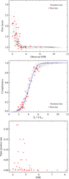 |
Fig. 2. Top panel: flux boosting factor versus observed S/N for simulated data (open circle) and real detections (red filled circle). Central panel: completeness as a function of the injected line flux Iin over the measured flux uncertainty ΔICO. The Iin for real detections are line fluxes that have been corrected for flux boosting factors in the top panel. The blue curve shows the best fit to the simulated data (see Eq. (3)). The completeness decreases with decreasing integrated flux normalized by noise, indicating that sources are more difficult to detect at low S/N. This analysis allows us to correct CO luminosity functions for the completeness of our search algorithm. Bottom panel: false positive rate versus S/N for CO detections in this study. |
where x = Iin/ΔICO. The best fit shows A = 4.1 and B = 1.6 in this study, which is shown in blue curve in Fig. 2. Given this tight correlation, we assign completeness and flux factors for each detection by matching it to a simulated source with the closest S/N, line flux, and rms level, as shown in Table 3. In the following analysis, we scale down the observed CO luminosities in all figures by the flux factors to account for flux boosting while still presenting flux factors and the observed flux and luminosities in tables. To obtain more conservative results, we did not scale down the flux and luminosity uncertainties.
Given that the simulations are computed for secure sources with a known position, this appears to be appropriate for the category A and B sources in our catalog. We note that one source in category C is detected with S/N = 3.8, which is lower than the S/N > 4 threshold applied in the simulations, we thus do not have constraints on its flux factor and completeness. We verified that including this source or not does not impact the following statistical analysis. Thus, we adopt the completeness and flux factors for category A and B sources and one source with S/N > 4 in category C.
In Fig. 2-bottom, we show the false positive rate of this sample. Among the 46 CO detections (Table 3), nine sources have well-matched optical spectroscopical redshifts to their CO redshifts which are solidly confirmed and false detection case can be excluded. The rest of the sources have no optical redshifts known. Some of them could be false positives, and counterparts can be found by chance within the 3″ search radius. The probability of false line detection can be conservatively estimated as 1 − RSoFiA, where the RSoFiA is the reliability computed from SoFiA. As the RSoFiA is computed from mosaics with similar resolutions, shallower than the large mosaic, the reliability of detection is actually higher than the SoFiA output, and the probability of false line detection (1 − RSoFiA) appears conservative. To constrain the probability of false counterparts, Pc, we ran simulations via randomly generating mocked sources with the same sky density of HST I and VLT Ks sources in this field, and searching for counterparts using a 3″ radius on a random position. We find that the false positive rate of HST I band counterparts is Pc = 0.46, and false Ks counterpart is Pc = 0.06. The false positive rate of HAE counterparts is entirely negligible, as the HAE sky density is lower than the HST I source density by two orders of magnitude, we thus assigned the false rate of HAE counterparts to 0. Therefore, the false positive rate Pfalse, that is, the probability of a counterpart being found by chance for a false line detection, is Pc × (1 − RSoFiA). As shown in Fig. 2-bottom, all sources in this sample have false positive rate < 0.24, and only sources with S/N < 5.5 have Pfalse > 0. The total false detection number (i.e., ΣPfalse, i) in this sample is less than 1.
4. Molecular gas content of the Spiderweb protocluster
Based on the source catalog presented in Sect. 3.3, we show the individual spectrum for each detection. Furthermore, we study the cold molecular gas properties of our sample including the determination of the CO(1−0) luminosity function of this high-density field.
4.1. Spectra and integrated CO maps
For all sources, we present the 1D-spectra and coutours of the integrated CO maps overlaid on optical/NIR images (see Fig. 3 and Appendix A). The integrated CO images are created by summing up the data cube between the channel ni and nj determined by MaxFinder (see Sect. 3.1), maximizing the S/N of the line and the visibility of the detection in integrated images. We emphasize that all detections are unresolved in the integrated CO images in which the contours are only used to highlight the S/N level and the optical counterpart. The non-Gaussian contours of some sources are due to the stacking of pointings with different resolutions that are not indicative for morphologies and do not affect the peak flux measurements on which the following analysis is based.
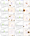 |
Fig. 3. ATCA spectra and integrated CO maps for detections with S/N > 5. Spectra panels: CO(1−0) lines are highlighted in green and fit by a single Gaussian profile shown by a blue curve. Reference names in Emonts et al. (2016) and Dannerbauer et al. (2017) are highlighted in blue when available. Image panels: optical images of 25″ × 25″ in size overlaid with CO(1−0) intensity contours. In general, images are taken from the HST F814W data (Miley et al. 2006), while VLT Ks (Dannerbauer et al. 2014) and Subaru z-band images (Koyama et al. 2013) are indicated as text in the upper right corner. Contours start at 2σ in steps of 1σ. |
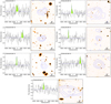 |
Fig. 3. continued. |
In Fig. 3, we present spectra of the 17 sources with S/N > 5 and their optical images overlaid with line intensity contours in which 16 of them have explicit counterparts in the optical/NIR imaging. The remaining source, that is, COALAS-SW.05, is serendipitously found at the edge of pointing SWpoint1 with CO(1−0) S/N = 5.9 at zspec = 2.189. This source is not covered by the VLT nor by HST imaging. However, we find a tentative counterpart in the Subaru z-band image (Koyama et al. 2013). Although there is high noise level at the edge of the pointing, it is unlikely to be spurious given the high S/N, thus we include it in the catalog.
4.2. Line identification and redshift distribution
In this study, all detected lines are identified as CO(1−0) at z ∼ 2.2. As shown in Table 3, nine sources are found with consistent redshifts to zCO(1 − 0) from NIR spectroscopy presented in Shimakawa et al. (2018) and/or the VLT/KMOS observations in Pérez-Martínez et al. (in prep., private consultation). Regarding the remaining sources without a secure spectroscopic redshift, in the case of higher-J CO transitions (e.g., CO(2−1) at z = 5.3), we inspected Herschel/SPIRE images for all CO detections and found no red colors that could suggest redshifts beyond z = 4 − 5 (e.g., Riechers et al. 2017). On the other hand, adopting the number density of z > 5 submillimeter galaxies in the COLDz survey (Riechers et al. 2020b), the expected number of z > 5 galaxies is less than 1 in this field. Thus, the detection of CO(2−1) appears very unlikely and cannot be used to constrain CO(2−1) space density at z = 5.3. We computed the CO(1−0) luminosities  following Solomon et al. (1997), namely
where SΔv is the integrated flux of the line in Jy km s−1 (corrected for flux boosting, see Sect. 3.4), DL is the luminosity distance in Mpc, and νobs is the observed frequency.
In Fig. 4, we show the redshift and CO(1−0) luminosity distribution, respectively. The detections spread over the redshift range z = 2.09 − 2.22 with CO(1−0) luminosity up to  = 2 × 10¹¹ K km s−1 pc2. Previous membership was based on Hα narrow-band imaging and subsequent NIR spectroscopy. Thus, the HAE redshift range of z = 2.146−2.170 is a selection effect of the narrow band filter NB2071 (Shimakawa et al. 2018) that is limited within the redshift range of z = 2.15 ± 0.2 and unable to probe the wider structure of the Spiderweb cluster. Strikingly, the CO emitters show an overdensity from z = 2.12 − 2.21, a factor of 3.8 wider in velocity than the range traced by the HAEs. Such an overdensity remains at z = 2.12 − 2.21 even if we limit the zCO histogram to only those sources with S/N > 5. It is independent of the rms level, line width, and other properties, which are robust and unlikely to be impacted by selection effects or misidentifications. Therefore, this indicates that this structure has a scale of 120 co-moving Mpc (cMpc), suggesting a filament and/or super structure. We discuss this further in Sect. 5.1.
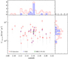 |
Fig. 4. CO luminosities versus redshifts for CO detections in this study. Top and right panels: redshift and CO luminosity distribution of our detections, respectively. In histograms, all CO emitters are shown in red, and HAEs with CO detections are shown in blue. |
4.3. Spatial distribution of CO emitters
In Fig. 5, we show the footprints of previous studies, including HST I band image, Subaru MOIRCS Ks band image (Koyama et al. 2013; Shimakawa et al. 2014) and LABOCA 870 μm continuum map. In this work, using ATCA we observed an area slightly larger than the HST F814W image, covering the majority of LABOCA sources in Dannerbauer et al. (2014) and HAEs in Koyama et al. (2013) and Shimakawa et al. (2014). As the R200 shown in green circle, the central cluster core around MRC1138 is well covered by all observations, while the large filamentary structure traced by HAEs is still not fully observed with ATCA.
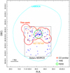 |
Fig. 5. Footprints of this work and previous studies, overlaid by CO sources (red circles) in this work and HAEs (blue crosses) in Koyama et al. (2013) and Shimakawa et al. (2018). The R200 radius (Shimakawa et al. 2014) is shown in a green circle centering on the MRC1138−262. |
In Fig. 6, we show the sky and velocity distributions of CO emitters in this study. Respectively, the left panel shows the velocity of CO emitters to their sky distance to the central radio galaxy MRC1138−262 while the right panel presents the normalized version. In Fig. 6-left, the CO emitters scatter largely in view of the observer, that is, in a line-of-sight velocity range of ±6500 km s−1 and at sky distances of 0 3−4
3−4 0 from the central galaxy. Robust sources (S/N > 5) are also found at large velocities (e.g., 5500 km s−1) and great distances (up to 3
 7) from the center, which further strengthens the large structure indicated by the large redshift range z = 2.12 − 2.21 of the CO overdensity (Sect. 4.2). Meanwhile, as indicated by the histogram in Fig. 6-left, 90% of the CO emitters are found to be at distances
  from the central radio galaxy. Thus, the single pointings of VLA or ATCA observations at 7 mm focusing on the center radio galaxy only cover 10% of CO sources presented in this work. Regarding the field of view of ALMA, only the ALMA compact array (ACA) at 3 mm can have a comparable primary beam (
 ) to the VLA and ATCA ones. Therefore, it is also impractical to discover large structures similar to the Spiderweb protocluster in single pointing mode. Hence, large area surveys (> 20 arcmin2) are essential to discover the majority of CO emitters in similar structures to those found in this study. On the other hand, narrow-band imaging can cover large areas (Koyama et al. 2013; Shimakawa et al. 2018) but the redshift range probed covers only 18% of the velocity range observed by ATCA, which is thus unable to discover such large structures.
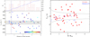 |
Fig. 6. Left panel: distribution of CO emitters versus their sky distances from the central radio galaxy MRC1138−262. Top panel: histogram (red) and cumulative fraction (blue) of CO emitters as a function of the distances to the center galaxy. Bottom panel: CO emitters are color-coded with their S/N. Gray shaded area marks the redshift range observed by the narrow band N2071 (Shimakawa et al. 2018) of MOIRCS at Subaru. Blue and black dashed lines mark the field of view of VLA and ATCA single pointings, respectively. Right panel: normalized velocity versus distance to center galaxy for CO emitters in this study and HAEs with a spectroscopic redshift (Shimakawa et al. 2018). The normalization factors are σ = 683 km s−1 and R200 = 0.53 Mpc (Table 2 in Shimakawa et al. 2014). The two dashed curves show the escape velocity (positive and negative) as a function of distance from the cluster mass 1.71 × 10¹⁴ M⊙ (Shimakawa et al. 2014) using the prescription of Rhee et al. (2017). Half of the CO emitters in this work have velocities outside of the region enclosed by these two curves that are not expected to be gravitationally bound to the central mass. |
Given the large velocity and spacial offsets from the center galaxy, some CO sources do not appear to be gravitationally bound to the center galaxy. In Fig. 6-right, we present the normalized velocity and distances to the center for CO emitters in this work and HAEs with spectroscopic redshifts (Shimakawa et al. 2018). Shimakawa et al. (2014) calculated a mass of 1.71 × 10¹⁴ M⊙ for the Spiderweb protocluster assuming virialization in the core. Using this mass, galaxies with velocities that fall within the region enveloped by the two curves (Rhee et al. 2017) are expected to be gravitationally bound. We find that 21 CO emitters have velocities inside the region enclosed by the two curves. In contrast, the remaining CO sources scatter largely in the diagram with velocities faster than the escape velocities, which are thus unlikely to be bound with the cluster core. They concluded that the two groups are not gravitationally bound to the core system and will remain distributed within the overall galaxy cluster. In this work, the velocities of CO emitters out of the bound region are one to five times larger than the escape velocities. Meanwhile, these unbound CO emitters are mostly at large distance (88% have R > R200), only four sources (including the center radio galaxy) are found within the R200 radius. This is in line with the picture drawn in Shimakawa et al. (2014), where the center is already collapsed and nearly virialized. The outer regions still appear highly structured, and some CO emitters could be at the early phase of assembly toward the protocluster core.
4.4. Comparison with previous surveys
This catalog contains 46 robust CO(1−0) detections, making it the largest catalog of CO emitters in a galaxy cluster field and among the largest ones ever published for one contiguous field. In Table 4, we compared this catalog to CO surveys from the literature in both high-z galaxy (proto)clusters and blank fields. To maintain consistency, we only show the number of detections that are found with counterparts in high-resolution images (e.g., HST, ALMA and VLA). In terms of the observed area, the 21 arcmin2 covered by ATCA is the largest one ever observed in protocluster fields to date, while the observed area of other surveys in protocluster fields are smaller by factors of 3−10. The number of 46 detected sources in the Spiderweb field is larger than the numbers presented in other protocluster works by a factor of 2−15. Thus, the CO emitter sample in this study constitutes the largest CO sample in a protocluster to date. We note that CO emitters in other protoclusters could be underestimated. As mentioned in Sect. 4.3, it is possible that other high-z protoclusters also contain a large number of CO emitters, but the majority of them would be missed due to the small area observed. This sample size is also comparable with respect to surveys in blank fields; for example, COLDz (Pavesi et al. 2018; Riechers et al. 2020a), ASPECS (González-López et al. 2019; Decarli et al. 2019), and PHiBSS2 (Lenkić et al. 2020). These CO surveys in blank fields have been used to constrain the CO luminosity function. Similarly, the large number of CO emitters with a significant overdensity in the Spiderweb cluster enables us to constrain the CO luminosity function and molecular gas density in an overdense region for the first time.
CO surveys in high-z clusters and blank fields.
4.5. CO(1–0) line width versus luminosity
The relationship between CO luminosity, and CO line width is an analog of the Tully–Fisher relation (Tully & Fisher 1977), which can be interpreted as a relationship between the molecular gas mass and the velocity necessary for centrifugal support of a rotating disk (Bothwell et al. 2013). Although showing a large scatter, this relation is a practical tool that enables us to indicatively diagnose the size and mass of gas reservoirs without high-resolution imaging.
In Fig. 7-top, we show the CO(1−0) luminosity  versus the FWHM of our detections. In addition, we include low-J CO observations, tracing the cold molecular gas of high-z galaxy (proto)clusters: CO(2−1) observations of a cluster at z = 1.46 (Hayashi et al. 2017) and CO(1−0) observations of two clusters at z = 1.62 and 2.51 (Rudnick et al. 2017; Wang et al. 2018), respectively. The CO(2−1) luminosities are converted into CO(1−0) luminosities using the brightness temperature ratio r21 = 0.76 (Daddi et al. 2015). CO emitters in Wang et al. (2018) and Hayashi et al. (2017) cover a wide parameter space on the plot, while other samples are limited to a smaller luminosity and FWHM range due to the small sample size and shallow depths. We show the parameterization of the
  versus FWHM relationship for a few representative cases: the relation for SMGs between these two parameters established by Bothwell et al. (2013) (radius = 7 kpc and αCO = 1), a disk model with a radius of 13 kpc from Dannerbauer et al. (2017), and a disk galaxy and a spherical model described in Aravena et al. (2019). The four lines have the same slope but different normalizations due to the assumption of a different disk radius and αCO. The relation of spherical models (i.e., with a small radius and low αCO) is above other models in larger disk sizes and high αCO. Compact galaxies with low αCO (e.g., starbursts) tend to have higher CO luminosity at fixed FWHM, while the
  –FWHM relations of typical disk galaxies tend to be lower than the relation of compact starbursts.
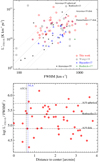 |
Fig. 7. Top panel: CO luminosity versus FWHM. CO detections in this study are shown in red circles with HAEs marked by blue crosses. The dashed lines are from Aravena et al. (2019) where the upper line represents a spherical model and the bottom line a disk model. ASPECS galaxies (Aravena et al. 2019) are shown in black pluses, which lie mostly along the disk model line. The solid line shows the relation from Bothwell et al. (2013) and the dot dashed line presents the disk model from Dannerbauer et al. (2017). Bottom panel: CO luminosity normalized by FWHM2 versus distance from the center galaxy. Vertical lines mark the half FWHM of ATCA (black) and VLA (blue) primary beams, respectively. This figure shows that CO emitters in the Spiderweb protocluster are more likely to be starbursts (mergers) compared to other high-z clusters, and these starbursts are beyond the field of view (FoV) of the single pointing focusing on the central galaxy. |
Interestingly, we find that a dozen CO sources show higher ratios of CO luminosity to line width compared to other galaxy cluster samples that are above the solid line for the disk model (Fig. 7-top) of Bothwell et al. (2013). Some members of the Spiderweb protocluster lie close to and/or even above the “spherical” model line presented in Aravena et al. (2019). Compared to other high-z cluster members, our cluster members have a larger CO luminosity at specific line width than the samples from Hayashi et al. (2017), Rudnick et al. (2017), and Wang et al. (2018). Overall, we find larger CO luminosities at fixed line width than all other previous surveys. We note that the optical/NIR images (see Fig. 3 and Appendix A) show that the morphologies of our cluster members are complex, and almost half of them appear irregular. The fit to the spherical CO gas models and their irregular morphology together suggest that these galaxies are merger-like systems, which is consistent with the expected high merger rate in galaxy cluster environments at high redshift (Coogan et al. 2018). Therefore, their  appears similar to SMGs suggesting that this cluster is rich of SMGs (and mergers) with respect to other high-z clusters. This further strengthens the conclusion presented in Dannerbauer et al. (2014).
In Fig. 7-bottom, we normalized the CO luminosity by FWHM2 as an indicator of starburstiness and show their sky distance from the center galaxy. Intriguingly, the most starburst-like galaxies, that is, sources above the spherical model in Aravena et al. (2019), are located  from the center galaxy. These galaxies would be totally missed in single pointing observations at 7 mm with ATCA and VLA if the phase center focused on the center cluster galaxy. Given that other surveys in protocluster fields are all observing a small area, the majority of starbursting members in protoclusters would be missed if the starbursting members were also far away from the center as in the Spiderweb. In this case, the starburst/merger rates in high-z protoclusters could be significantly underestimated due to the limited field of view. This work indicates that conventional single pointing observations could have severe bias in protocluster fields that missed the bulk of starbursting members.
4.6. CO(1–0) luminosity function
Our large CO(1−0) sample enables us to establish the CO luminosity function and study the molecular gas density in a galaxy protocluster environment for the first time. We constructed the CO luminosity function adopting Eq. (2) from Decarli et al. (2016):
where Ni is the number of galaxies that fall within the luminosity bin log Li − 0.25 and log Li + 0.25, Vc is defined as the observed co-moving volume, Cj is the completeness described in Sect. 3.4 and Rj is the reliability. We note that Lenkić et al. (2020) introduced two association probabilities to weight each detection. These are the probability of an optical counterpart associated with a particular CO transition Pz, j and the probability of a line detection spatially associated with an optical counterpart Pa, j. However, in this study, Pz, j is equal to 1 as all lines are identified as CO(1−0), and Pa, j is close to 1 because we used tolerance < 3″ to match any optical counterpart. The uncertainty of spatial association is negligible with respect to 5−13″ beam sizes. Therefore, we adhered to the equation by Decarli et al. (2019). We adopted R = 1 for a source with a counterpart and a matching of a previously known/obtained spectroscopic redshift. In cases of sources without a spectroscopic redshift, we conservatively treated the reliability from SoFiA as upper limits. In each luminosity bin, the CO space densities are created 1000 times, each time the reliability Rj is distributed to a random value that is uniformly distributed between 0 and such upper limit (see also González-López et al. 2019; Pavesi et al. 2018; Riechers et al. 2019). Line candidates were only kept in our analysis if the random value was below the reliability threshold. The final CO luminosity functions are the medians of all the CO LF realizations, and the uncertainty was computed as Poissonian uncertainty  .
.
In order to calculate the volume, we first defined the redshift range of this cluster as z = 2.146 − 2.17 (i.e., 33 co-moving Mpc or ±1200 km s−1) being determined by the redshift range of the HAEs in this cluster (Fig. 4). This redshift range is also consistent with the z = 2.15 − 2.17 used in Dannerbauer et al. (2014) for calculating the SFRD, which enabled us to consistently compare the CO space density to the SFRD. The total sky coverage of the ATCA mosaic is 25.8 arcmin2. We excluded shallow areas that have rms noise > 1 mJy per beam where no source is detected there, and thus we adopted 21.3 arcmin2, that is, 53 cMpc2. We also computed the CO luminosity function for detections at the redshift range z = 2.12 − 2.21 (124 cMpc), as an overdensity of CO emitters is also seen within this redshift range (Fig. 4). Therefore, the observed co-moving volume is ∼6600 cMpc3 for the redshift range z = 2.12 − 2.21 and ∼1650 cMpc3 for z = 2.146 − 2.17, respectively. We show the CO number densities for the two redshift ranges in Fig. 8 and Table 5. The CO luminosity function was calculated in luminosity bins of 0.5 dex width to compare consistently with the COLDz luminosity function, starting log( /K km s−1 pc2) = 10.1 in steps of 0.1 dex. The log(
 /K km s−1 pc2) < 10.1 bins were ignored because of the small sample size and high level of incompleteness. The CO space density at z = 2.146 − 2.17 is consistent with the one at z = 2.12 − 2.21 within error bars (Fig. 8-right). We note that the narrow redshift range z = 2.146 − 2.17 is also comparable with the gravitationally bound region in Fig. 6-right, the similar amplitudes of CO luminosity functions in the two redshift ranges indicate that the CO space density is not enhanced in the gravitationally bound region of the cluster core. Given that the larger number of sources found in the wide redshift range can better constrain the CO luminosity function than is done with the narrower redshift range, we thus adopt the CO luminosity function at z = 2.12 − 2.21 for further analysis.
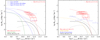 |
Fig. 8. CO(1−0) luminosity functions for the Spiderweb protocluster and samples from the literature. Left: CO(1−0) luminosity density in each luminosity bin at z = 2.12 − 2.21 in this work, compared with the results at z ∼ 2 from the COLDz (Riechers et al. 2019) and predictions from semi-analytic SHARK models (Lagos et al. 2012, 2020). The dotted-dashed black lines mark the fifth and 95th percentiles of the COLDz luminosity function. The red dashed curve shows the best fit to our data. We show CO luminosity functions for protoclusters derived from SHARK models within two different volumes. One (blue dashed curve) is calculated in a spherical volume with radius R < 5 cMpc and the other one (blue dot-dashed curve) is in the identical volume to that where the observed CO luminosity function is measured, respectively. Right: same as the left panel, but boxes are shown for CO luminosity density in a narrow redshift range z = 2.146 − 2.17. Blue arrows mark the lower limits for protoclusters in Zavala et al. (2019), and the orange curve shows the results from Vallini et al. (2016). |
CO(1−0) luminosity function.
Furthermore, we verified the CO luminosity function for robust sources (S/N > 5) at z = 2.12 − 2.21. We found that the median amplitude of CO luminosity function would be scaled down by 0.5 dex due to it having fewer galaxies per luminosity bin but still being one order of magnitude higher than that for COLDz, and it agrees with the density of the full sample within error bars. On the other hand, given that S/N > 5 sources are robustly detected, using their reliability as upper limits appears too conservative, we thus directly adopted their reliability from SoFiA as the Rj in Eq. (5) and found that the resulting CO luminosity function for > 5σ sources is in excellent agreement with the best fit (Fig. 8-left). Therefore, these confirm that our CO luminosity function results are robust and even conservative.
We fit the observed CO(1−0) luminosity function of z = 2.12 − 2.21 with a Schechter function (Schechter 1976) in the logarithmic form used in Riechers et al. (2019):
where Φ* is the scale number of galaxies per unit co-moving volume (in units of cMpc−3 dex−1),  is the scale line luminosity in units of K km s−1 pc2 (the “knee” of the luminosity function), and α is the slope of the faint end. We show the best-fit results for CO luminosity function at z = 2.12 − 2.21 in Table 6, including one fit with free parameters and two with fixed slopes. The best fit with free Schechter parameters has α = −0.21 ± 1.13, log(
 /K km s−1 pc2) = 10.48 ± 0.38 and log Φ* = −2.16 ± 0.49. We note that the slope of the faint end of the luminosity function, α, is very uncertain due to the limited number of galaxies. This parameter is sensitive to the corrections we applied for reliability and completeness.
Schechter function fit parameter constraints to CO(1−0) luminosity function at 2.12 < z < 2.21.
In order to consistently compare our result with studies from the literature, we fit the CO luminosity function with fixed values of α in our analysis, adopting α = 0.08 from the COLDz CO(1−0) luminosity function (Riechers et al. 2019) and α = −0.2 from the ASPECS project (Decarli et al. 2019), respectively. As listed in Table 6, the best fit with fixed α = 0.08 shows log( /K km s−1 pc2) = 10.39 ± 0.06 and log Φ* = −2.06 ± 0.07. The log L* is close to the COLDz log(
 /K km s−1 pc2) = 10.7 (50th percentile), while the CO number density Φ* in this study is 2.6 ± 0.5 dex higher than COLDz number density. If we adopt α = −0.2 as in Decarli et al. (2019), we would obtain log(
 /K km s−1 pc2) = 10.48 ± 0.07 and log Φ* = −2.16 ± 0.09 – the density is still more than one order of magnitude higher than the estimated one in COLDz. Comparing with number densities Φ* from ASPECS (Decarli et al. 2019), our results are higher than ASPECS CO(3−2) density at z ∼ 2.6 by 1.4 ± 0.5 dex. To summarize, the fits with fixed slopes show a consistent scaled line luminosity log(
 /K km s−1 pc2) ∼ 10.5 and number density (log Φ* ∼ −2.2) to the fit with free parameters. All fits on our sample show more than 1.5 dex higher number density of CO emitters than the COLDz and ASPECS surveys.
For comparison, we added data from the literature: the observed CO luminosity functions from the field galaxy sample COLDz (Riechers et al. 2019) and Vallini et al. (2016). The CO luminosity density in the Spiderweb protocluster is remarkably higher than that in field galaxy samples; for example, 1.3−1.6 orders of magnitude higher than the median value in COLDz survey at log( /K km s−1 pc2)∼10.5, and 3.4 orders of magnitude higher than the results from Vallini et al. (2016). Recently, Zavala et al. (2019) provided a constraint on gas content in protoclusters at z ∼ 2.0 − 2.5 based on ALMA continuum observations which show enhanced gas density in protocluster environments. Our results agree well with the lower limits in Zavala et al. (2019). Furthermore, we compare with results from the semi-analytic models in Lagos et al. (2012, 2020) predicted for both the random field and the overdense environment. We refer the reader to a detailed discussion on the comparison in Sect. 5.2.
4.7. Molecular gas density in the Spiderweb protocluster
In general, the cold molecular gas density can be obtained by integrating the CO(1−0) luminosity functions and applying a fixed CO to H2 conversion factor αCO for all CO emitters. However, the αCO of these CO emitters are uncertain. Some CO emitters appear to be starbursts (see Sect. 4.5) that have lower αCO than that applied for field galaxies (e.g., αCO = 3.6 M⊙ (K km s−1 pc2)−1 in Riechers et al. 2019; Decarli et al. 2019). In order to have a reasonable conversion to cold molecular gas mass, we applied two typical αCO values for starbursts and normally star-forming galaxies that are diagnosed by the  –FWHM diagram, respectively. For the 19 CO sources above the Bothwell et al. (2013) line in Fig. 7, we adopted a starburst-like αCO = 0.8 M⊙ (K km s−1 pc2)−1 (Emonts et al. 2018) and adopted αCO = 3.6 M⊙ (K km s−1 pc2)−1 (Daddi et al. 2010) for the rest of sources that appear to be disk-like. Given that Wang et al. (2018) adopted αCO ⪆ 4.0 M⊙ (K km s−1 pc2)−1 in the z = 2.5 starbursting clusters (determined following Genzel et al. 2015), the values applied in this work are conservative.
In order to calculate the cold molecular gas density, we followed three different methods: (1) we simply summed up the CO(1−0) luminosity of all detections at z = 2.12 − 2.21 in our catalog (taking into account the flux boosting) and converted it into the cold molecular gas using the bimodal αCO described above, and by dividing the total cold molecular gas mass by the co-moving volume, we obtained a cold molecular gas density ρ(H2) = 5.9 × 10⁸ M⊙ cMpc−3; (2) we derived the cold molecular gas density by adopting a similar method to that presented in Decarli et al. (2016), summing up and weighting the gas mass of each CO detection by completeness and reliability, as we did for the calculation of the CO luminosity function (Sect. 4.6), that is,
where Mj is the gas mass the jth galaxy calculated as  (we obtained a high value for the cold molecular gas density
  cMpc−3 with uncertainties of the fifth and 95th percentiles); (3) assuming the same CO luminosity function slope as the COLDz work, we derived the cold gas density by scaling up the COLDz CO(1−0) luminosity function to our work. The COLDz project (Riechers et al. 2019) reported a cold molecular gas density of 1.1 − 5.6 × 10⁷ M⊙ cMpc−3 at z ∼ 2, assuming αCO = 3.6 M⊙ (K km s−1 pc2)−1. The COLDz CO(1−0) luminosity function (50th percentile) shows log(
 /K km s−1 pc2) = 10.7, log Φ* = −3.87 and α = −0.08. Compared to our Schechter function fit with the same slope (Table 6), our CO luminosity function is 1.7 ± 0.06 dex higher in scaled number density and 0.2 ± 0.05 dex lower in scaled luminosity. The integrated Schechter function is
  . Thus, the cold molecular gas density in this protocluster would be 1.5 orders of magnitude higher than that in the COLDz survey, that is,
  Mpc−3 adopting the same αCO = 3.6. This calculation would be scaled down by a factor of 1.3 if adopting the bimodal αCO described above. We note that calculations (1) and (2) are based only on the observed part of the luminosity function, and undetected galaxies in lower luminosity bins are not accounted for the given large uncertainties in the individual luminosity bins and the unknown intrinsic shape of the CO luminosity function. The three calculations agree well with each other, while the estimate (2) appears conservative but consistent with the results of (1) and (3). We thus adopted the calculation (2) and estimated the H2 density ρ(H2) = 0.56 − 1.26 × 10⁹ M⊙ Mpc−3 in the Spiderweb galaxy protocluster.
In Fig. 9, we compare the cold molecular gas density with results from the COLDz (Riechers et al. 2019) and ASPECS (Decarli et al. 2016, 2019) surveys. Similarly to the CO luminosity function, the H2 density in the Spiderweb cluster is two orders of magnitude higher than that determined in field galaxy samples, such as COLDz and ASPECS. We note that the ASPECS H2 densities (Decarli et al. 2019) based on CO(3−2) with assumed r31 = 0.42 ± 0.07 should be scaled down by a factor of two, on average, as calibrated by VLA CO(1−0) follow-ups (Riechers et al. 2020a), which have recently been updated in Decarli et al. (2020), adopting r31 = 0.84 ± 0.26 from Riechers et al. (2020a). The H2 density in this galaxy protocluster is completely based on CO(1−0), the best tracer of the cold molecular gas and free from CO excitation issues.
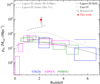 |
Fig. 9. H2 density of this study (the red star) compared to results from COLDz (Riechers et al. 2019), ASPECS (Decarli et al. 2020), and PHIBSS2 (Lenkić et al. 2020) overlaid by the fitting of field galaxy samples from Liu et al. (2019) and Lagos et al. (2020). Gas density in galaxy clusters from simulations are shown via gray curves for SHARK (Lagos et al. 2020) in two volumes, and a gray diamond with a bar for DIANOGA (Bassini et al. 2020), respectively. The gray diamond with the error bar shows the median, and the downward triangle marks the maximum values for cluster structures in DIANOGA simulations. The gas density in this work is significantly higher than observed in blank fields and also higher than predictions for clusters in simulations. |
An important caveat is that the H2 density strongly depends on the adopted αCO. Here, we adopted a bimodal αCO. Although this is a good representation of the full sample, the value of αCO for individual galaxies can be highly uncertain.
5. Discussion
5.1. Is the Spiderweb a super-protocluster?
The redshift range of the CO emitters (z = 2.12 − 2.21) is a factor of four wider than the redshift range of HAEs and LAEs in this field and indicates a size of 124 Mpc in co-moving distance along the line of sight. Kurk et al. (2000) conducted narrow-band Lyα imaging in this field using the VLT/FORS. They used a narrow-band filter with a central wavelength of 381.4 nm and a FWHM of 6.5 nm, covering a redshift range of z = 2.111 − 2.164. Pentericci et al. (2000) followed up the LAEs selected from Kurk et al. (2000) with the VLT/FORS in MOS mode. They confirmed reshifts of Lyα emitters mostly at z = 2.14 − 2.17 except one quasar at z = 2.183 with a Lyα absorption feature. Kuiper et al. (2011) discovered a sample of satellite galaxies around the center galaxy MRC1138−262 while detecting Hα, [O II] and [O III] emissions with SINFONI spectroscopy. Their redshifts span z = 2.13 − 2.17, which is larger than the redshift range of narrow-band-selected HAEs (Koyama et al. 2013; Shimakawa et al. 2018). Both the LAEs and HAEs selected in this field are limited on a narrow redshift range due to the use of narrow-band filters. The velocity distribution of the confirmed satellite galaxies shows a broad, double-peaked velocity structure with σ = 1013 ± 87 km s−1, which is proposed to be a result of the merger of two subclusters (Kuiper et al. 2011). Including all spectroscopically confirmed HAEs and LAEs, Shimakawa et al. (2014) measured a velocity dispersion of 683 km s−1 in the cluster core with a R200 = 0.53 Mpc in physical distance. However, in this study, the CO emitters show a much larger spread in redshifts and sky that cannot be interpreted as an effect of pure velocity dispersion of cluster galaxies as it would lead to an unrealistically large dispersion exceeding 4000 km s−1. Furthermore, since robust sources (S/N > 5, Fig. 6) are found to be at high velocities (e.g., 5500 km s−1) and great distances (e.g., 3 7), the large spread of velocities and distances to the center cannot be explained as a selection effect. Thus, we argue that the large redshift range of CO emitters is tracing a large-scale structure that is significantly wider than the previously assumed one. Overall, the CO emitters provide us with a very different view of the protocluster structure than that of Lyα and Hα emitters and appear to be better tracers of the large-scale matter density.
The ∼120 Mpc co-moving size is significantly larger than the scale of any known galaxy (proto)clusters at low and high redshift, beside the supercluster Hyperion (Cucciati et al. 2018) that is found with a radial size of 150 cMpc. We note that the overdensity of CO emitters at z = 2.12 − 2.21 is only slightly higher than the density of the remaining redshift range covered by the ATCA. This structure could be larger than what we observed and more comparable to the radial scale of the Hyperion. This might indicate that we observe a galaxy super-protocluster similar to the Hyperion (Cucciati et al. 2018). However, given that the 53 cMpc2 area covered by ATCA is 72 times smaller than the 60 × 60 cMpc2 size of the Hyperion, this structure could possibly be a protocluster connected to a large-scale filamentary structure along the line of sight. We are not able to distinguish if this structure is a filament or a super-protocluster with the current data in hand. In case of a super-protocluster, such a large structure appears unlikely to totally collapse by z = 0, given that half of the CO emitters in this study appear not bound to the central mass (Fig. 6-right). This also holds for the Hyperion. However, filaments can act as highways to fuel the inner regions of clusters with gas and galaxies, as indicated by the ThreeHundred simulations (Rost et al. 2021). There, filaments around clusters can extend out to five R200 and are comparable to the distances between the CO emitters and the center core in this study. Thus, the collapse of the gas and dark matter would be accelerated if it is a protocluster connected to a large-scale filament.
The volume observed in this work is very elongated (∼6 × 9 × 120 cMpc3), thus it is difficult, with such a narrow field of view, to decide whether the structure may be filamentary. In order to confirm the filamentary or super-protocluster structure, a comprehensive redshift survey covering a large area is of utmost importance. Emonts et al. (2018) reported six CO(4−3) and four [CI](1−0) detections using ALMA observations around the MRC1138−262. These observations took only 106 min integration time (in a single ALMA pointing). Very recently, Valentino et al. (2020) showed the impressive capabilities of ALMA to obtain CO and [CI] transitions in a few minutes of on-source integration time for a sample of a few tens of high-z IR-selected galaxies. In the Spiderweb protocluster field, high-resolution ALMA observations of alternative molecular gas tracer, for example, [CI] (accompanying CO(4−3) line emission), would be invaluable to constrain SFEs of individual galaxies and the gas excitation via constructing CO SLEDs. The detection rate in the Spiderweb field would be more complete with ALMA given the high brightness of CO(4−3) with respect to CO(1−0). The bandwith of ALMA band 4 is two times wider than the 2 GHz bandwidth of ATCA. However, given that the CO(4−3) line is at a 4× higher frequency than CO(1−0), the redshift range probed by ALMA band 4 is just half of the range probed by ATCA, thus making it less efficient in probing the large scale of this structure. Therefore, benefiting from its large field of view and broad bandwidth, ATCA is still the best facility for CO line surveys with the largest volumes. In the near future, the upgraded graphics processor units4 on ATCA will double the amount of bandwidth that can be observed, and hence future ATCA observations of the Spiderweb field will be crucial to unveiling the edge of this large structure.
5.2. Comparison to simulations
In Fig. 8, we compared our results with CO luminosity functions in the SHARK semi-analytic models for both field and cluster environments (Lagos et al. 2020). For the field, we compared with GALFORM (Lagos et al. 2012) and SHARK (Lagos et al. 2018, 2020). To compare with our protocluster, we searched for halos with masses > 1013.5 M⊙ in the latest SHARK simulations (Lagos et al. 2020) and selected the CO(1−0) emitters that fall within the same volume (and geometry) of the Spiderweb protocluster. We find that the CO luminosity function of this protocluster is characterized by a higher number density than the SHARK predictions for both the field and clusters. Compared to the COLDz CO luminosity function, SHARK (Lagos et al. 2020) predicts a CO luminosity function with a different shape, which has a lower number density at bright luminosities, > 1010.5 K km s−1 pc2 and higher number density at low luminosities. The CO luminosity function of Spiderweb has a more similar shape that resembles the SHARK one for the field but with a remarkably higher number density, by 2.3 dex at log( /K km s−1 pc2) = 10.5. To make a fairer comparison with the Spiderweb, we investigated the CO luminosity function of high-mass halos in SHARK using two different volumes: (1) a spherical volume of R < 5 cMpc, which is representative of cluster cores, marked by the blue dashed curve; and (2) the identical volume and geometry of the observed co-moving volume (6600 cMpc3) in this work, marked by blue dot-dashed curve. As shown in Fig. 8-left, the small-volume CO luminosity function of SHARK (R < 5 cMpc core) is comparable to the one observed in the Spiderweb protocluster, but it appears to have a slightly too high number density at the brightest end (though with poor statistics it is hard to assess whether this is a true tension with the prediction). However, when we study the CO luminosity function adopting the same comoving volume as we used for the Spiderweb, the number density decreases by 0.6 dex across all luminosities. This indicates that cold molecular gas reservoirs in the simulated SHARK clusters are overdense in center cluster cores, yet much lower in the outer regions. This could indicate that this protocluster is in a higher density region of the Universe than the average halo of mass > 1013.5 M⊙ at z = 2 in SHARK.
In Fig. 9, we compare our cold molecular gas densities with predictions for clusters from the SHARK semi-analytical models (Lagos et al. 2020) and the DIANOGA hydrodynamical simulations (Bassini et al. 2020), respectively. The core region (R < 5 cMpc) of massive halos in SHARK shows a median gas density of  cMpc−3 at z = 2 with a median αCO of 1.23, indicating a high density of starburst-like members in the center core. This gas density in the core region is still lower than the bottom limit of our result by a factor of 2. In the identical volume and geometry to the one analyzed in this paper (this Vc), the SHARK models predict a molecular gas density of
  cMpc−3 at z = 2, which is lower than the observed one by 1.3 dex, even when accounting for uncertainties of αCO. In the DIANOGA simulations, which consist of a set of 12 cosmological simulations of massive galaxy clusters (see Bassini et al. 2020 for further details), there is no direct information on the molecular gas content. We thus compare to the cold gas content that directly fuel the star formation of cluster galaxies. Between the 12 simulations, we selected the one with the highest gas density at z ∼ 2. This is a simulation of a massive cluster with a mass M200 > 1015 M⊙ at z = 0. Therefore, this simulation is suitable for this comparison, since numerical simulations suggest that the Spiderweb complex is the progenitor of a very massive galaxy cluster at z = 0 (e.g., Saro et al. 2009). For this simulated cluster, we chose the snapshot nearest to the redshift of the Spiderweb protocluster and computed the gas density considering all the cold gas bound to the galaxies within the same volume and geometry. By employing ∼10 000 randomly chosen lines of sight, we find a median density of
  cMpc−3 (16th and 84th percentiles) with a maximum of 1.29 × 10⁹ M⊙ cMpc−3 for massive structures with M500 > 1015 M⊙ at z = 2.16 (Saro et al. 2009). The median gas density agrees with the observed one within the error bar, and the maximum density is very comparable with the upper limit of our results.
Most of the simulations and semi-analytical models underpredict the star formation rate in protoclusters at z ∼ 2 and 4 (e.g., Granato et al. 2015; Bassini et al. 2020; Lim et al. 2021). This work shows that the molecular gas density in protoclusters can also be underestimated in the SHARK simulations. Regarding the tension between the observations and the SHARK models, one possibility would be that the Spiderweb protocluster is of a much higher density than the one typically traced by halos of masses > 1013.5 M⊙ in simulations, and hence we are not comparing like for like. In the future, we will investigate if any of the massive halos in these simulations can produce the correct density of star-forming galaxies (and which cosmological volume is required to see such high densities). After pinpointing whether those systems exist in the simulations, follow-up investigations will focus on comparing star formation efficiencies and their spatial distribution within the protocluster environment. On the other side, the DIANOGA simulations contain more massive structures similar to the Spiderweb protocluster, providing very comparable gas density predictions with respect to our observations. We note that even though the total gas densities are comparable, the gas mass function could be different between the observations and simulations. A detailed study on gas mass function requires a deeper inspection, which is beyond the scope of this study. To summarize, this comparison shows that observed high-z super-protocluster and large filamentary structures do exist in cosmological simulations, and the consistency with observations provides encouraging prospects for future simulation studies.
5.3. SFRD versus gas density
Based on submillimeter imaging with APEX-LABOCA, Dannerbauer et al. (2014) report that the SFRD of this structure is 1500 M⊙ yr−1 Mpc−3 in physical volume, corresponding to a SFRD = 47 M⊙ yr−1 cMpc−3 in co-moving volume after applying a scaling factor of (1 + z)3. This SFRD is higher than the cosmic SFRD in random fields by 2.6 dex (see a review in Madau & Dickinson 2014).
Intriguingly, our observations suggest that the H2 density is 1.6 ± 0.5 orders of magnitude higher than in the field, which is lower than the 2.6 orders of magnitude excess of SFRD with respect to that in blank fields. The offset could be due to a combination of several reasons: (1) a high SFE of the cluster members as suggested by the high fraction of dusty starbursts in this structure; (2) an overestimation of the SFRs due to blending as the dusty SEDs in Dannerbauer et al. (2014) are based on low-resolution Herschel and LABOCA (sub)millimeter photometry that could boost the SFR measurements; (3) the H2 density could be underestimated due to the lack of constraint at the faint end of CO luminosity function; and (4) we might be missing some CO emitters in noisy regions. In order to better constrain the LIR and SFRs of individual galaxies, deblended photometry (e.g., Jin et al. 2018; Liu et al. 2018) and wide and deep spectral-line imaging (by ATCA and ALMA) would be essential to identify the main contributors to the difference between the SFRD and the H2 density of this structure.
5.4. The importance of large area surveys with wide velocity ranges
As listed in Table 4, previous cold molecular gas surveys often observe a small area around the protocluster (core). In contrast, the Spiderweb protocluster exhibits large distances between CO emitters and the center galaxy (Fig. 6), indicating that such large structures can only be revealed by large area line surveys. Other high-z protoclusters could have a similarly large spread of gas reservoirs to the Spiderweb protocluster; however, most CO emitters in such structures would be missed by surveys that cover small areas and narrow velocity ranges, resulting in an underestimate of the total gas mass and gas density. Clearly, large area surveys (> 10 armin2) are indispensable to unveil complete cluster members and unbiased gas content in high-z protoclusters. The area needs to be even larger for super structures like the Spiderweb and the Hyperion. However, a blind line survey appears inefficient and risky, as the existence of CO emitters is unknown in the outskirts of the protocluster. To improve the efficiency, the single-dish (sub)millimeter observations are valuable; for example, APEX/LABOCA, JCMT/SCUBA2, IRAM 30 m/NIKA2 and the upcoming LMT/TolTEC. All these instruments can trace the dust content in protoclusters with large fields of view. As demonstrated in this work and Hill et al. (2020), the ATCA and ALMA follow-up of LABOCA submillimeter sources around the cluster core will increase the efficiency of line surveys. On the other hand, the CO(1−0) detection rate of HAEs in this field is 17%, which is comparable to that reported by Tadaki et al. (2014). Thus, CO line follow-up observations covering most of the rest-frame UV/optical line emitters also appears to be a good strategy for future surveys. A detailed analysis on CO(1−0)-detected HAEs in this field will be presented in future work (Jin et al., in prep.).
6. Conclusion
We present new ATCA CO observations of the z = 2.16 Spiderweb galaxy protocluster field. We find 46 robust CO(1−0) emitting sources at the redshift of the Spiderweb protocluster. For the first time, we place constraints on the CO luminosity function and the cold molecular gas density on a galaxy protocluster environment in the distant Universe. Our findings can be summarized as follows:
-
475 h integration time was spent on observations of the CO(1−0) transition of members of the Spiderweb protocluster at z = 2.16. We produced a large mosaic of 13 pointings at 7 mm, covering an area of 25 arcmin2 and velocity range of ±7000 km s−1. Using multiple source extraction methods, we reveal 46 solid CO(1−0) detections with S/N > 4 and counterparts in HST optical and/or VLT NIR images.
-
The CO emitters span a redshift range of z = 2.09 − 2.22. We find a CO overdensity at z = 2.12 − 2.21, which is four times larger than the velocity range traced by HAEs in previous studies and suggests a large-scale filament or a galaxy super-protocluster in this field.
-
We find that 90% of the CO emitters are
 distant from the central radio galaxy, indicating that line surveys with small areas would miss the bulk of CO sources in similar structures. Meanwhile, half of the CO emitters are found to have velocities larger than the escape velocities, assuming the virialization of the cluster core, which appears not gravitationally bound to the center mass. These unbound CO emitters extend to 4 × R200 but are barely found within the R200 radius, which is consistent with the picture that the cluster core has been virialized and the outer regions are still in formation.
 -
Compared to high-redshift protoclusters known in the literature, this structure contains more CO emitters with relatively narrow line width and high luminosity, which is consistent with SMG samples and indicates starburst/merger activities. The most starburst-like members have large sky distances to the center galaxy with
 , which is beyond the FoV of single pointings of VLA and ATCA. This indicates that small area observations could have severe bias in protocluster fields missing a bulk of starbursting members.
 -
We construct the CO luminosity function in this cluster, and find a high overdensity of luminous CO sources. The amplitude of the luminosity function, log(Φ*/cMpc−3 dex−1) = −2.16 ± 0.49, is 1.6 ± 0.5 orders of magnitude higher than the CO luminosity density in blank fields, and also higher than the prediction from semi-analytical SHARK models by one order of magnitude. This indicates a high density of cold molecular gas 0.6 − 1.3 × 10⁹ M⊙ cMpc−3, which is significantly higher than that probed for field galaxy samples by more than one order of magnitude. This gas density is also higher than predictions by semi-analytical SHARK models for protoclusters, while it is comparable with the cold gas density in the hydrodynamical DIANOGA simulations. We attribute the underprediction of SHARK partially to the lack of very high density regions in their simulated box, ∼(300 Mpc)3.
To summarize, this study shows that molecular line surveys in high-z protoclusters are more efficient than surveys in blank fields, and line surveys with large area and wide velocity ranges are of utmost importance to providing an unbiased view of large structures and gas content in protocluster environments, and thus test our understanding of galaxy formation and numerical simulations.
See SoFiA control parameter at https://github.com/SoFiA-Admin/SoFiA/wiki/SoFiA-Control-Parameters
Acknowledgments
The Australia Telescope Compact Array is part of the Australia Telescope National Facility which is funded by the Australian Government for operation as a National Facility managed by CSIRO. We acknowledge the Gomeroi people as the traditional owners of the Observatory site. This work is making use of observations made with ESO Telescopes at Paranal under programme 088.A-0754(B), 091.A-0106(A) and 094.A-0104(A). This research is based on observations made with the NASA/ESA Hubble Space Telescope obtained from the Space Telescope Science Institute, which is operated by the Association of Universities for Research in Astronomy, Inc., under NASA contract NAS 5-26555. These observations are associated with program 10327. The authors thank Ian Smail, Stefano Borgani and Elena Rasia for helpful discussions in the preparation of this manuscript. The authors acknowledge Bärbel Koribalski for help on ATCA observations and introduction of SoFiA. The authors thank Laura Lenkić and Alberto D. Bolatto for helpful discussions on CO luminosity function. SJ, HD, and JMR acknowledge financial support from the Spanish Ministry of Science, Innovation and Universities (MICIU) under grant AYA2017-84061-P, co-financed by FEDER (European Regional Development Funds) and the Agencia Estatal de Investigación del Ministerio de Ciencia e Innovación (AEI-MCINN) under grant (La evolución de los cúmulos de galaxias desde el amanecer hasta el mediodía cósmico) with reference (PID2019-105776GB-I00/DOI:10.13039/501100011033). HD acknowledges financial support from the Spanish Ministry of Economy and Competitiveness (MINECO) under the 2014 Ramón y Cajal program MINECO RYC-2014-15686. BE acknowledges official funding from the National Radio Astronomy Observatory. The National Radio Astronomy Observatory is a facility of the National Science Foundation operated under cooperative agreement by Associated Universities, Inc. CL is funded by the ARC Centre of Excellence for All Sky Astrophysics in 3 Dimensions (ASTRO 3D), through project number CE170100013. LB acknowledges ExaNeSt and Euro Exa projects, funded by the European Union Horizon 2020 research and innovation program under grant agreement No. 671553 and No. 754337, the agreement ASI-INAF n.2017-14-H.0; DIANOGA simulations have been carried out using MENDIETA Cluster from CCAD-UNC, which is part of SNCAD-MinCyT (Argentina); MARCONI at CINECA (Italy), with CPU time assigned through grants ISCRA B, and through INAF-CINECA and University of Trieste – CINECA agreements; at the Tianhe-2 platform of the Guangzhou Supercomputer Center by the support from the National Key Program for Science and Technology Research and Development (2017YFB0203300). The post-processing has been performed using the PICO HPC cluster at CINECA through an expression of interest. JBC thanks the National Science Foundation for support through grants AST-1714528 and AST-1814034, and additionally the University of Texas at Austin College of Natural Sciences. CMC thanks the National Science Foundation for support through grants AST-1814034 and AST-2009577, the University of Texas at Austin College of Natural Sciences, and the Research Corporation for Science Advancement from a 2019 Cottrell Scholar Award sponsored by IF/THEN, an initiative of Lyda Hill Philanthropies.
References
- Aravena, M., Decarli, R., Gónzalez-López, J., et al. 2019, ApJ, 882, 136 [CrossRef] [Google Scholar]
- Bassini, L., Rasia, E., Borgani, S., et al. 2020, A&A, 642, A37 [NASA ADS] [CrossRef] [EDP Sciences] [Google Scholar]
- Béthermin, M., Fudamoto, Y., Ginolfi, M., et al. 2020, A&A, 643, A2 [CrossRef] [EDP Sciences] [Google Scholar]
- Bothwell, M. S., Smail, I., Chapman, S. C., et al. 2013, MNRAS, 429, 3047 [Google Scholar]
- Casey, C. M. 2016, ApJ, 824, 36 [NASA ADS] [CrossRef] [EDP Sciences] [Google Scholar]
- Castignani, G., Combes, F., Salomé, P., et al. 2019, A&A, 623, A48 [NASA ADS] [CrossRef] [EDP Sciences] [Google Scholar]
- Chabrier, G. 2003, PASP, 115, 763 [Google Scholar]
- Champagne, J. B., Casey, C. M., Zavala, J. A., et al. 2021, ApJ, 913, 110 [NASA ADS] [CrossRef] [Google Scholar]
- Chiang, Y.-K., Overzier, R. A., Gebhardt, K., & Henriques, B. 2017, ApJ, 844, L23 [NASA ADS] [CrossRef] [Google Scholar]
- Coogan, R. T., Daddi, E., Sargent, M. T., et al. 2018, MNRAS, 479, 703 [NASA ADS] [Google Scholar]
- Cucciati, O., Lemaux, B. C., Zamorani, G., et al. 2018, A&A, 619, A49 [NASA ADS] [CrossRef] [EDP Sciences] [Google Scholar]
- Daddi, E., Elbaz, D., Walter, F., et al. 2010, ApJ, 714, L118 [Google Scholar]
- Daddi, E., Dannerbauer, H., Liu, D., et al. 2015, A&A, 577, A46 [NASA ADS] [CrossRef] [EDP Sciences] [Google Scholar]
- Dannerbauer, H., Daddi, E., Riechers, D. A., et al. 2009, ApJ, 698, L178 [NASA ADS] [CrossRef] [Google Scholar]
- Dannerbauer, H., Kurk, J. D., De Breuck, C., et al. 2014, A&A, 570, A55 [NASA ADS] [CrossRef] [EDP Sciences] [Google Scholar]
- Dannerbauer, H., Lehnert, M. D., Emonts, B., et al. 2017, A&A, 608, A48 [NASA ADS] [CrossRef] [EDP Sciences] [Google Scholar]
- Davies, J. I., Bianchi, S., Baes, M., et al. 2014, MNRAS, 438, 1922 [NASA ADS] [CrossRef] [Google Scholar]
- Decarli, R., Walter, F., Aravena, M., et al. 2016, ApJ, 833, 69 [Google Scholar]
- Decarli, R., Walter, F., Gónzalez-López, J., et al. 2019, ApJ, 882, 138 [Google Scholar]
- Decarli, R., Aravena, M., Boogaard, L., et al. 2020, ApJ, 902, 110 [Google Scholar]
- Dressler, A. 1980, ApJ, 236, 351 [NASA ADS] [CrossRef] [Google Scholar]
- Dunlop, J. S., McLure, R. J., Biggs, A. D., et al. 2017, MNRAS, 466, 861 [Google Scholar]
- Emonts, B. H. C., Feain, I., Röttgering, H. J. A., et al. 2013, MNRAS, 430, 3465 [NASA ADS] [CrossRef] [Google Scholar]
- Emonts, B. H. C., Norris, R. P., Feain, I., et al. 2014, MNRAS, 438, 2898 [NASA ADS] [CrossRef] [Google Scholar]
- Emonts, B. H. C., Lehnert, M. D., Villar-Martín, M., et al. 2016, Science, 354, 1128 [NASA ADS] [CrossRef] [Google Scholar]
- Emonts, B. H. C., Lehnert, M. D., Dannerbauer, H., et al. 2018, MNRAS, 477, L60 [NASA ADS] [CrossRef] [Google Scholar]
- Genzel, R., Tacconi, L. J., Lutz, D., et al. 2015, ApJ, 800, 20 [Google Scholar]
- Gómez-Guijarro, C., Riechers, D. A., Pavesi, R., et al. 2019, ApJ, 872, 117 [NASA ADS] [CrossRef] [Google Scholar]
- González-López, J., Decarli, R., Pavesi, R., et al. 2019, ApJ, 882, 139 [CrossRef] [Google Scholar]
- Gooch, R. 1996, in Astronomical Data Analysis Software and Systems V, eds. G. H. Jacoby, & J. Barnes, ASP Conf. Ser., 101, 80 [Google Scholar]
- Granato, G. L., Ragone-Figueroa, C., Domínguez-Tenreiro, R., et al. 2015, MNRAS, 450, 1320 [NASA ADS] [CrossRef] [Google Scholar]
- Hatch, N. A., Overzier, R. A., Röttgering, H. J. A., Kurk, J. D., & Miley, G. K. 2008, MNRAS, 383, 931 [NASA ADS] [CrossRef] [Google Scholar]
- Hayashi, M., Kodama, T., Kohno, K., et al. 2017, ApJ, 841, L21 [NASA ADS] [CrossRef] [Google Scholar]
- Hill, R., Chapman, S., Scott, D., et al. 2020, MNRAS, 495, 3124 [CrossRef] [Google Scholar]
- Ivison, R. J., Papadopoulos, P. P., Smail, I., et al. 2011, MNRAS, 412, 1913 [Google Scholar]
- Ivison, R. J., Biggs, A. D., Bremer, M., Arumugam, V., & Dunne, L. 2020, MNRAS, 496, 4358 [CrossRef] [Google Scholar]
- Jin, S., Daddi, E., Liu, D., et al. 2018, ApJ, 864, 56 [Google Scholar]
- Jin, S., Daddi, E., Magdis, G. E., et al. 2019, ApJ, 887, 144 [Google Scholar]
- Koyama, Y., Kodama, T., Tadaki, K.-I., et al. 2013, MNRAS, 428, 1551 [CrossRef] [Google Scholar]
- Kuiper, E., Hatch, N. A., Miley, G. K., et al. 2011, MNRAS, 415, 2245 [NASA ADS] [CrossRef] [Google Scholar]
- Kurk, J. D., Röttgering, H. J. A., Pentericci, L., et al. 2000, A&A, 358, L1 [NASA ADS] [Google Scholar]
- Kurk, J. D., Pentericci, L., Röttgering, H. J. A., & Miley, G. K. 2004, A&A, 428, 793 [NASA ADS] [CrossRef] [EDP Sciences] [Google Scholar]
- Lagos, C. D. P., Bayet, E., Baugh, C. M., et al. 2012, MNRAS, 426, 2142 [NASA ADS] [CrossRef] [Google Scholar]
- Lagos, C. D. P., Tobar, R. J., Robotham, A. S. G., et al. 2018, MNRAS, 481, 3573 [CrossRef] [Google Scholar]
- Lagos, C. D. P., da Cunha, E., Robotham, A. S. G., et al. 2020, MNRAS, 499, 1948 [CrossRef] [Google Scholar]
- Lee, M. M., Tanaka, I., Kawabe, R., et al. 2019, ApJ, 883, 92 [CrossRef] [Google Scholar]
- Lenkić, L., Bolatto, A. D., Förster Schreiber, N. M., et al. 2020, AJ, 159, 190 [CrossRef] [Google Scholar]
- Lim, S., Scott, D., Babul, A., et al. 2021, MNRAS, 501, 1803 [CrossRef] [Google Scholar]
- Liu, D., Gao, Y., Isaak, K., et al. 2015, ApJ, 810, L14 [NASA ADS] [CrossRef] [Google Scholar]
- Liu, D., Daddi, E., Dickinson, M., et al. 2018, ApJ, 853, 172 [Google Scholar]
- Liu, D., Schinnerer, E., Groves, B., et al. 2019, ApJ, 887, 235 [Google Scholar]
- Madau, P., & Dickinson, M. 2014, ARA&A, 52, 415 [NASA ADS] [CrossRef] [Google Scholar]
- Miley, G. K., Overzier, R. A., Zirm, A. W., et al. 2006, ApJ, 650, L29 [NASA ADS] [CrossRef] [Google Scholar]
- Miller, T. B., Chapman, S. C., Aravena, M., et al. 2018, Nature, 556, 469 [NASA ADS] [CrossRef] [Google Scholar]
- Muldrew, S. I., Hatch, N. A., & Cooke, E. A. 2015, MNRAS, 452, 2528 [NASA ADS] [CrossRef] [Google Scholar]
- Noble, A. G., McDonald, M., Muzzin, A., et al. 2017, ApJ, 842, L21 [Google Scholar]
- Noble, A. G., Muzzin, A., McDonald, M., et al. 2019, ApJ, 870, 56 [NASA ADS] [CrossRef] [Google Scholar]
- Oteo, I., Ivison, R. J., Dunne, L., et al. 2018, ApJ, 856, 72 [Google Scholar]
- Overzier, R. A. 2016, A&ARv, 24, 14 [NASA ADS] [CrossRef] [Google Scholar]
- Pavesi, R., Sharon, C. E., Riechers, D. A., et al. 2018, ApJ, 864, 49 [Google Scholar]
- Pentericci, L., Kurk, J. D., Röttgering, H. J. A., et al. 2000, A&A, 361, L25 [NASA ADS] [Google Scholar]
- Rhee, J., Smith, R., Choi, H., et al. 2017, ApJ, 843, 128 [NASA ADS] [CrossRef] [Google Scholar]
- Riechers, D. A., Leung, T. K. D., Ivison, R. J., et al. 2017, ApJ, 850, 1 [Google Scholar]
- Riechers, D. A., Pavesi, R., Sharon, C. E., et al. 2019, ApJ, 872, 7 [Google Scholar]
- Riechers, D. A., Boogaard, L. A., Decarli, R., et al. 2020a, ApJ, 896, L21 [Google Scholar]
- Riechers, D. A., Hodge, J. A., Pavesi, R., et al. 2020b, ApJ, 895, 81 [Google Scholar]
- Rigby, E. E., Hatch, N. A., Röttgering, H. J. A., et al. 2014, MNRAS, 437, 1882 [NASA ADS] [CrossRef] [Google Scholar]
- Rost, A., Kuchner, U., Welker, C., et al. 2021, MNRAS, 502, 714 [Google Scholar]
- Rudnick, G., Hodge, J., Walter, F., et al. 2017, ApJ, 849, 27 [Google Scholar]
- Saro, A., Borgani, S., Tornatore, L., et al. 2009, MNRAS, 392, 795 [CrossRef] [Google Scholar]
- Sault, R. J., Teuben, P. J., & Wright, M. C. H. 1995, in Astronomical Data Analysis Software and Systems IV, eds. R. A. Shaw, H. E. Payne, & J. J. E. Hayes, ASP Conf. Ser., 77, 433 [Google Scholar]
- Schechter, P. 1976, ApJ, 203, 297 [Google Scholar]
- Serra, P., Jurek, R., & Flöer, L. 2012, PASA, 29, 296 [NASA ADS] [CrossRef] [Google Scholar]
- Serra, P., Westmeier, T., Giese, N., et al. 2015, MNRAS, 448, 1922 [Google Scholar]
- Shimakawa, R., Kodama, T., Tadaki, K.-I., et al. 2014, MNRAS, 441, L1 [NASA ADS] [CrossRef] [Google Scholar]
- Shimakawa, R., Koyama, Y., Röttgering, H. J. A., et al. 2018, MNRAS, 481, 5630 [CrossRef] [Google Scholar]
- Smail, I., Dudzevičiūtė, U., Stach, S. M., et al. 2021, MNRAS, 502, 3426 [CrossRef] [Google Scholar]
- Solomon, P. M., Downes, D., Radford, S. J. E., & Barrett, J. W. 1997, ApJ, 478, 144 [Google Scholar]
- Spergel, D. N., Verde, L., Peiris, H. V., et al. 2003, ApJS, 148, 175 [NASA ADS] [CrossRef] [Google Scholar]
- Spergel, D. N., Bean, R., Doré, O., et al. 2007, ApJS, 170, 377 [NASA ADS] [CrossRef] [Google Scholar]
- Spérone-Longin, D., Jablonka, P., Combes, F., et al. 2021, A&A, 647, A156 [CrossRef] [EDP Sciences] [Google Scholar]
- Stach, S. M., Swinbank, A. M., Smail, I., et al. 2017, ApJ, 849, 154 [NASA ADS] [CrossRef] [Google Scholar]
- Tadaki, K.-I., Kodama, T., Tamura, Y., et al. 2014, ApJ, 788, L23 [NASA ADS] [CrossRef] [EDP Sciences] [Google Scholar]
- Tadaki, K.-I., Kodama, T., Hayashi, M., et al. 2019, PASJ, 71, 40 [NASA ADS] [CrossRef] [Google Scholar]
- Tully, R. B., & Fisher, J. R. 1977, A&A, 500, 105 [Google Scholar]
- Valentino, F., Daddi, E., Puglisi, A., et al. 2020, A&A, 641, A155 [CrossRef] [EDP Sciences] [Google Scholar]
- Vallini, L., Gruppioni, C., Pozzi, F., Vignali, C., & Zamorani, G. 2016, MNRAS, 456, L40 [Google Scholar]
- Walter, F., Decarli, R., Aravena, M., et al. 2016, ApJ, 833, 67 [Google Scholar]
- Wang, T., Elbaz, D., Daddi, E., et al. 2016, ApJ, 828, 56 [NASA ADS] [CrossRef] [Google Scholar]
- Wang, T., Elbaz, D., Daddi, E., et al. 2018, ApJ, 867, L29 [NASA ADS] [CrossRef] [Google Scholar]
- Wang, T., Schreiber, C., Elbaz, D., et al. 2019, Nature, 572, 211 [Google Scholar]
- Yajima, Y., Sorai, K., Miyamoto, Y., et al. 2021, PASJ, 73, 257 [CrossRef] [Google Scholar]
- Zavala, J. A., Casey, C. M., Scoville, N., et al. 2019, ApJ, 887, 183 [CrossRef] [Google Scholar]
Appendix A: Gallery of CO(1–0) detections
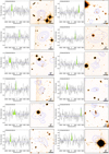 |
Fig. A.1. continued. |
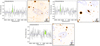 |
Fig. A.1. continued. |
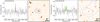 |
Fig. A.2. Spectra and intensity maps of category-C detections. |
All Tables
Schechter function fit parameter constraints to CO(1−0) luminosity function at 2.12 < z < 2.21.
All Figures
|
Fig. 1. S/N map of line candidates (Sect. 3.1) in the ATCA mosaic. The S/N is the maximum S/N computed in the 1D spectrum on each pixel by our algorithm MaxFinder (see details in Sect. 3.1). The color bar values are limited in 1.5 < S/N < 6.5 for fair visibility of detections. ATCA pointings are shown in gray circles with a radius of 0.9′. Gray solid circles mark the pointings MRC1138 in Emonts et al. (2016) and HAE229 in Dannerbauer et al. (2017), respectively. The cyan contour encloses the area with rms < 1 mJy beam−1. Detected sources are marked by solid the following solid color circles: blue: category A; magenta: category B; green: category C (see details in Sect. 3.3). |
| In the text | |
|
Fig. 2. Top panel: flux boosting factor versus observed S/N for simulated data (open circle) and real detections (red filled circle). Central panel: completeness as a function of the injected line flux Iin over the measured flux uncertainty ΔICO. The Iin for real detections are line fluxes that have been corrected for flux boosting factors in the top panel. The blue curve shows the best fit to the simulated data (see Eq. (3)). The completeness decreases with decreasing integrated flux normalized by noise, indicating that sources are more difficult to detect at low S/N. This analysis allows us to correct CO luminosity functions for the completeness of our search algorithm. Bottom panel: false positive rate versus S/N for CO detections in this study. |
| In the text | |
|
Fig. 3. ATCA spectra and integrated CO maps for detections with S/N > 5. Spectra panels: CO(1−0) lines are highlighted in green and fit by a single Gaussian profile shown by a blue curve. Reference names in Emonts et al. (2016) and Dannerbauer et al. (2017) are highlighted in blue when available. Image panels: optical images of 25″ × 25″ in size overlaid with CO(1−0) intensity contours. In general, images are taken from the HST F814W data (Miley et al. 2006), while VLT Ks (Dannerbauer et al. 2014) and Subaru z-band images (Koyama et al. 2013) are indicated as text in the upper right corner. Contours start at 2σ in steps of 1σ. |
| In the text | |
|
Fig. 3. continued. |
| In the text | |
|
Fig. 4. CO luminosities versus redshifts for CO detections in this study. Top and right panels: redshift and CO luminosity distribution of our detections, respectively. In histograms, all CO emitters are shown in red, and HAEs with CO detections are shown in blue. |
| In the text | |
|
Fig. 5. Footprints of this work and previous studies, overlaid by CO sources (red circles) in this work and HAEs (blue crosses) in Koyama et al. (2013) and Shimakawa et al. (2018). The R200 radius (Shimakawa et al. 2014) is shown in a green circle centering on the MRC1138−262. |
| In the text | |
|
Fig. 6. Left panel: distribution of CO emitters versus their sky distances from the central radio galaxy MRC1138−262. Top panel: histogram (red) and cumulative fraction (blue) of CO emitters as a function of the distances to the center galaxy. Bottom panel: CO emitters are color-coded with their S/N. Gray shaded area marks the redshift range observed by the narrow band N2071 (Shimakawa et al. 2018) of MOIRCS at Subaru. Blue and black dashed lines mark the field of view of VLA and ATCA single pointings, respectively. Right panel: normalized velocity versus distance to center galaxy for CO emitters in this study and HAEs with a spectroscopic redshift (Shimakawa et al. 2018). The normalization factors are σ = 683 km s−1 and R200 = 0.53 Mpc (Table 2 in Shimakawa et al. 2014). The two dashed curves show the escape velocity (positive and negative) as a function of distance from the cluster mass 1.71 × 10¹⁴ M⊙ (Shimakawa et al. 2014) using the prescription of Rhee et al. (2017). Half of the CO emitters in this work have velocities outside of the region enclosed by these two curves that are not expected to be gravitationally bound to the central mass. |
| In the text | |
|
Fig. 7. Top panel: CO luminosity versus FWHM. CO detections in this study are shown in red circles with HAEs marked by blue crosses. The dashed lines are from Aravena et al. (2019) where the upper line represents a spherical model and the bottom line a disk model. ASPECS galaxies (Aravena et al. 2019) are shown in black pluses, which lie mostly along the disk model line. The solid line shows the relation from Bothwell et al. (2013) and the dot dashed line presents the disk model from Dannerbauer et al. (2017). Bottom panel: CO luminosity normalized by FWHM2 versus distance from the center galaxy. Vertical lines mark the half FWHM of ATCA (black) and VLA (blue) primary beams, respectively. This figure shows that CO emitters in the Spiderweb protocluster are more likely to be starbursts (mergers) compared to other high-z clusters, and these starbursts are beyond the field of view (FoV) of the single pointing focusing on the central galaxy. |
| In the text | |
|
Fig. 8. CO(1−0) luminosity functions for the Spiderweb protocluster and samples from the literature. Left: CO(1−0) luminosity density in each luminosity bin at z = 2.12 − 2.21 in this work, compared with the results at z ∼ 2 from the COLDz (Riechers et al. 2019) and predictions from semi-analytic SHARK models (Lagos et al. 2012, 2020). The dotted-dashed black lines mark the fifth and 95th percentiles of the COLDz luminosity function. The red dashed curve shows the best fit to our data. We show CO luminosity functions for protoclusters derived from SHARK models within two different volumes. One (blue dashed curve) is calculated in a spherical volume with radius R < 5 cMpc and the other one (blue dot-dashed curve) is in the identical volume to that where the observed CO luminosity function is measured, respectively. Right: same as the left panel, but boxes are shown for CO luminosity density in a narrow redshift range z = 2.146 − 2.17. Blue arrows mark the lower limits for protoclusters in Zavala et al. (2019), and the orange curve shows the results from Vallini et al. (2016). |
| In the text | |
|
Fig. 9. H2 density of this study (the red star) compared to results from COLDz (Riechers et al. 2019), ASPECS (Decarli et al. 2020), and PHIBSS2 (Lenkić et al. 2020) overlaid by the fitting of field galaxy samples from Liu et al. (2019) and Lagos et al. (2020). Gas density in galaxy clusters from simulations are shown via gray curves for SHARK (Lagos et al. 2020) in two volumes, and a gray diamond with a bar for DIANOGA (Bassini et al. 2020), respectively. The gray diamond with the error bar shows the median, and the downward triangle marks the maximum values for cluster structures in DIANOGA simulations. The gas density in this work is significantly higher than observed in blank fields and also higher than predictions for clusters in simulations. |
| In the text | |
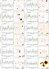 |
Fig. A.1. Spectra of S/N = 4 − 5 detections in category A. This figure shares the caption of Fig. 3. |
| In the text | |
|
Fig. A.1. continued. |
| In the text | |
|
Fig. A.1. continued. |
| In the text | |
|
Fig. A.2. Spectra and intensity maps of category-C detections. |
| In the text | |
Current usage metrics show cumulative count of Article Views (full-text article views including HTML views, PDF and ePub downloads, according to the available data) and Abstracts Views on Vision4Press platform.
Data correspond to usage on the plateform after 2015. The current usage metrics is available 48-96 hours after online publication and is updated daily on week days.
Initial download of the metrics may take a while.