| Issue |
A&A
Volume 652, August 2021
|
|
|---|---|---|
| Article Number | A25 | |
| Number of page(s) | 17 | |
| Section | Galactic structure, stellar clusters and populations | |
| DOI | https://doi.org/10.1051/0004-6361/202039951 | |
| Published online | 04 August 2021 | |
Abundance–age relations with red clump stars in open clusters⋆,⋆⋆
1
Laboratoire d’Astrophysique de Bordeaux, Univ. Bordeaux, CNRS, B18N, allée Geoffroy Saint-Hilaire, 33615 Pessac, France
e-mail: laia.casamiquela-floriach@u-bordeaux.fr
2
Núcleo de Astronomía, Facultad de Ingeniería y Ciencias, Universidad Diego Portales, Av. Ejército 441, Santiago, Chile
3
Leibniz-Institut für Astrophysik Potsdam (AIP), An der Sternwarte 16, 14482 Potsdam, Germany
4
Institut UTINAM, CNRS UMR6213, Univ. Bourgogne Franche-Comté, OSU-THETA Franche-Comté-Bourgogne, Observatoire de Besançon, BP 1615 25010 Besançon Cedex, France
5
INAF-Osservatorio Astronomico di Padova, vicolo dell’Osservatorio 5, 35122 Padova, Italy
6
Dept. FQA, Institut de Ciéncies del Cosmos (ICCUB), Universitat de Barcelona (IEEC-UB), Martí Franqués 1, 08028 Barcelona, Spain
7
Harvard-Smithsonian Center for Astrophysics, 60 Garden Street, Cambridge, MA 02138, USA
Received:
19
November
2020
Accepted:
14
May
2021
Context. Precise chemical abundances coupled with reliable ages are key ingredients to understanding the chemical history of our Galaxy. Open clusters (OCs) are useful for this purpose because they provide ages with good precision.
Aims. The aim of this work is to investigate the relation between different chemical abundance ratios and age traced by red clump (RC) stars in OCs.
Methods. We analyzed a large sample of 209 reliable members in 47 OCs with available high-resolution spectroscopy. We applied a differential line-by-line analysis, performing a comprehensive chemical study of 25 chemical species. This sample is among the largest samples of OCs homogeneously characterized in terms of atmospheric parameters, detailed chemistry, and age.
Results. In our metallicity range (−0.2 < [M/H] < +0.2) we find that while most Fe-peak and α elements show a flat dependence on age, the s-process elements show a decreasing trend with increasing age with a remarkable knee at 1 Gyr. For Ba, Ce, Y, Mo, and Zr, we find a plateau at young ages (< 1 Gyr). We investigate the relations between all possible combinations among the computed chemical species and age. We find 19 combinations with significant slopes, including [Y/Mg] and [Y/Al]. The ratio [Ba/α] shows the most significant correlation.
Conclusions. We find that the [Y/Mg] relation found in the literature using solar twins is compatible with the one found here in the solar neighborhood. The age–abundance relations in clusters at large distances(d > 1 kpc) show larger scatter than those in clusters in the solar neighborhood, particularly in the outer disk. We conclude that, in addition to pure nucleosynthetic arguments, the complexity of the chemical space introduced by the Galactic dynamics must be taken into account in order to understand these relations, especially outside of the local bubble.
Key words: stars: abundances / open clusters and associations: general / techniques: spectroscopic
Full Tables A.1 and A.2 are only available in electronic form at the CDS via anonymous ftp to cdsarc.u-strasbg.fr (130.79.128.5) or via http://cdsarc.u-strasbg.fr/viz-bin/cat/J/A+A/652/A25
© L. Casamiquela et al. 2021
 Open Access article, published by EDP Sciences, under the terms of the Creative Commons Attribution License (https://creativecommons.org/licenses/by/4.0), which permits unrestricted use, distribution, and reproduction in any medium, provided the original work is properly cited.
1. Introduction
To advance towards a broader understanding of the chemical evolution of the Milky Way, detailed element abundances from high-quality spectroscopic data and precise ages are needed (Soderblom 2010; Jofré et al. 2019). Stars change their chemical composition via several nucleosynthesis processes, particularly during their deaths, and this leads to the evolution of the overall chemical composition of their host galaxy. Newly synthesized elements will be inherited to form the next generation of stars, which ultimately guides the chemical evolution of the Universe (see Freeman & Bland-Hawthorn 2002; Matteucci 2012, for reviews). Therefore, the dependency of different elemental abundances with time is one of the most informative constraints shaping chemical evolution models.
It is usually assumed that the measured atmospheric chemical abundances are representative of the chemical pattern of the interstellar medium at the birthplace of stars. However, there are some processes that take place during the lifetime of a star that may change their atmospheric abundances. For instance, in FGK low-mass stars, internal transport processes (e.g., rotation-induced mixing, convection, atomic diffusion, internal gravity waves, or thermohaline mixing) can alter the surface abundances of some chemical species such as Li and Be (see e.g., Smiljanic et al. 2016; Lagarde et al. 2017; Charbonnel et al. 2020). However, the overall consensus is that, broadly speaking, chemical abundances of heavier elements measured in the spectra of low-mass stars remain constant during their lifetime, and reflect the chemical composition of their birth clouds.
Studying the temporal evolution of the chemical composition of reliable tracers at different regimes of age, metallicity, and Galactic location is crucial to understanding the variables that control Galactic evolution, such as supernovae yields, the star formation rate, or feedback mechanisms (Matteucci 2012; Maiolino & Mannucci 2019). The fact that not all chemical elements are produced in the same way or in the same timescale across cosmic times means that we must use a variety of chemical abundance ratios to disentangle the different processes affecting galaxy evolution. Moreover, it has proven useful to classify the chemical abundances into families according to their main production sites and nucleosynthetic channels: iron-peak, α-elements, light elements, odd-Z, and neutron-capture elements. So far, the abundance ratio relating the α-capture with the iron-peak family ([α/Fe]) has been widely considered as a proxy for the age of stellar populations in different Galactic studies (e.g., Minchev et al. 2013). However, it is important to keep in mind that there is scatter in the [α/Fe]–age relation in any location of the Milky Way that can be attributed to the mixture of stellar populations (Chiappini et al. 2015; Anders et al. 2018; Miglio et al. 2021).
Some other abundance ratios of elements coming from different families could be more informative for chemical evolution investigations because they can show even stronger dependence on stellar age than the [α/Fe] ratio. These abundance ratios were recently dubbed “chemical clocks” (Nissen 2015). Indeed, da Silva et al. (2012), and later Nissen (2015), performed very high-precision abundance analyses of solar twins, finding a linear trend of [Y/Mg] versus age with a slope of ∼0.04 dex Gyr−1. These latter authors propose that this slope reflects the timescale of production of both elements: α−elements (like Mg) are produced by massive stars on a short timescale, while neutron-capture elements produced by the s-process (like Y) are mainly synthesized by intermediate-mass stars. The different timescales imply that as time goes on, [Y/Mg] changes significantly more than other abundance ratios.
This relation was further confirmed by Tucci Maia et al. (2016) and Spina et al. (2018) with larger samples of solar twins also analyzed with very high precision. However, when studied in solar-type stars as a function of metallicity (Feltzing et al. 2017), the relation vanishes towards lower metallicities, placing a lower limit of [Fe/H] ∼ −0.5 for the relation to become flat. Later, Delgado Mena et al. (2019), Titarenko et al. (2019), and Casali et al. (2020) also noticed a possible nonuniversality of most chemical clocks at different metallicities, spatial location, and different Galactic populations (e.g., the thick disk). Recently, Magrini et al. (2021) proposed a theoretical explanation involving magnetic mixing.
To test the behavior of chemical clocks, it is important to study stars with equivalently precise ages and abundances, but outside the Local Bubble. An interesting approach to reaching a large spatial volume with precise abundances is to analyze giant stars, but reliable ages are in general difficult to obtain, and particularly at large distances (see Soderblom 2010, for a review). The most reliable methods for obtaining ages are those based on stellar evolution models, namely isochrone placing or asteroseismology, which presumably are those that depend on the fewest assumptions. Isochrone placement becomes challenging for individual field stars, and uncertainties in the atmospheric parameters and degeneration of the models usually hinder attempts to obtain precise ages. Fortunately, placing isochrones is often much easier in clusters because they have many coeval mono-metallic members and so the results are very precise, which is why, historically, they provide the primary benchmarks we use to study age-related properties (see Friel et al. 2013, for a review). Asteroseismic ages can be complementary to isochrone ages, as they can be precise (∼30% Valentini et al. 2019; Miglio et al. 2021) for giants, where isochrone ages cannot give a precise age given the proximity of the evolutionary tracks in the red giant branch.
Open clusters (OCs) provide an interesting alternative to solar twins for testing chemical clocks because their age and distance determinations are much more accurate and precise than for field stars at the same distances. Also, the fact that OCs are chemically homogeneous, at least up to ∼0.02 dex (Liu et al. 2016; Casamiquela et al. 2020), allows for a much more precise chemical abundance determination when several members are observed per cluster, as we see in the present study. This is why they have been used extensively to trace the Galactic thin disk abundance patterns (e.g., Magrini et al. 2017; Donor et al. 2018; Casamiquela et al. 2019).
Slumstrup et al. (2017) showed that the [Y/Mg] versus age relation obtained in the literature seems to be also followed by red clump giants in four OCs, although these latter authors used one star per cluster. Recently, Casamiquela et al. (2020, hereafter Paper I) complemented this study by analyzing several red giants from a further three clusters. These clusters also nicely followed the trend of [Y/Mg] versus age reported in the literature. However, when Casali et al. (2020) calculated “chemical ages” from their relation obtained from their 500 solar analogs on a sample of 19 OCs from the Gaia-ESO Survey, and compared these ages with those obtained from isochrone fitting, they did not find robust agreement for all clusters. These latter authors concluded that the chemical clocks broke for some of their innermost clusters (RGC < 7 kpc), pointing towards a nonuniversality in the [s/α]–[Fe/H]–age relationship.
Following Gaia DR2 (Gaia Collaboration 2018b), new reliable memberships of previously known and newly discovered OCs were reported (e.g., Cantat-Gaudin et al. 2018; Castro-Ginard et al. 2018, 2019, 2020). Cantat-Gaudin et al. (2020, CG20 hereafter) derived ages using an automatic data-driven approach from Gaia photometry and parallaxes for 1867 OCs. This sample offers a perfect opportunity to study the trends between chemical abundance and age for a large number of OCs covering a much larger area of the Galaxy than reached with solar analog field stars. In this paper, we present our findings from analyses combining this latest set of OCs – with precise ages – with high precision differential abundances obtained from high-resolution spectral analyses.
We organize the paper as follows. In Sect. 2 we detail the sample of clusters, their membership selections, and the origin of the spectroscopic data, the pipeline used to perform the spectroscopic analysis, and details of the atmospheric parameters. In Sect. 3 we describe the computation of the differential chemical abundances and their uncertainties. The OC ages are discussed in Sect. 4. In Sect. 5 we present the cluster chemical abundances [X/Fe] as a function of age. In Sect. 6 we analyze the possible combinations of abundance ratios that show a significant linear correlation with age. We discuss the obtained linear relations of the [Y/Mg] and [Y/Al] chemical clocks and compare these with the literature. In Sect. 6.2 we discuss the effects of using an extended sample of clusters outside of the solar neighborhood in the abundance–age relations. Finally, our conclusions are presented in Sect. 7.
2. The spectroscopic sample
2.1. Target selection and spectra
In this study, we selected the clusters from the revisited list of CG20, which includes ages, distances, and extinctions (see an in-depth discussion of the ages in Sect. 4).
We made a selection of nearby clusters (d ∼ 500 pc): being close by, these clusters tend to be well detached from the field distribution in proper motion and parallax, and their membership selection is usually very reliable. We used membership selections of OCs based on Gaia DR2 provided by Gaia Collaboration (2018a) and Cantat-Gaudin et al. (2018), and we selected the targets according to their positions in the color–magnitude diagram (CMD) (in a wide region around the red clump). The selected stars are usually bright and so archival data are usually available. We searched for high-resolution and high-signal-to-noise-ratio (S/N) spectra of the stars from public archives in eight different spectrographs: UVES@VLT, FEROS@2.2m MPG/ESO, HARPS@3.6m ESO, HARPS-N@TNG, FIES@NOT, ESPaDOnS@CFHT, NARVAL@TBL, and ELODIE@1.93m OHP (more details of the used instruments are explained in Paper I). We collected spectra corresponding to 151 stars in 11 clusters. Additionally, we performed our own observing programs with the spectrograph NARVAL@TBL over two semesters (2018B, 2019A). We observed 31 stars in four different clusters. These spectra were reduced using the standard reduction pipeline in NARVAL.
We added to our sample the spectra observed in the framework of the OCCASO survey (Casamiquela et al. 2016, 2019), in which the OCs cover a wide range of age and Galactocentric radius. In this case, we selected the highest S/N spectra observed by OCCASO from the spectrographs HERMES@Mercator and FIES@NOT (Observatorio del Roque de los Muchachos). Before the analysis, we already rejected the stars identified as nonmembers or spectroscopic binaries in the subsample of OCCASO analyzed by (Casamiquela et al. 2019). Our analysis pipeline succeeded for 236 spectra in this subsample, corresponding to 219 stars in 39 OCs. Several clusters in this sample also had stars with spectra in public archives.
2.2. Radial velocities and atmospheric parameters
To perform the analysis of the spectra we used the public spectroscopic software iSpec (Blanco-Cuaresma et al. 2014; Blanco-Cuaresma 2019). We make use of the same pipeline built in Paper I (we refer the reader to that paper for further details). Briefly, the strategy goes as follows:
– As a first step, the spectra coming from the different instruments are homogenized by cutting them to a common wavelength range (480–680 nm), and downgraded to a common spectral resolution (45 000). After the determination of radial velocities using a cross-correlation algorithm, telluric regions and emission lines due to cosmics are masked, and a normalization is performed using a median and maximum filtering.
– Afterwards, we use the spectral-synthesis fitting method to compute atmospheric parameters (Teff, log g, [M/H], [α/M], and vmic). The fitting is done by comparing the uncertainty-weighted fluxes of a set of observed features with a synthetic spectrum. Atmospheric parameters are varied until convergence of a least-squares algorithm is reached. The whole process made use of the local thermodynamic equilibrium (LTE) radiative transfer code SPECTRUM (Gray & Corbally 1994) and the MARCS atmospheric models (Gustafsson et al. 2008). We used the Gaia-ESO line list (Heiter et al. 2015).
Individual uncertainties in the radial velocities, atmospheric parameters, and abundances are computed by our pipeline. Figure 1 shows the dependence of the uncertainties in the atmospheric parameters on S/N. Their mean values are 0.045 dex in log g, and 18 K in Teff. Uncertainties are also slightly dependent on the temperature of the star: colder stars exhibit lower uncertainties at a given S/N.
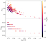 |
Fig. 1. Uncertainties in the retrieved Teff (top) and log g (bottom) as a function of S/N. The colors show the computed log Teff. |
Zeropoints among instruments. To account for systematic offsets between the different instruments, we analyzed the computed atmospheric parameters of stars observed with several instruments. In Paper I, we performed the same analysis and found no systematic difference above the quoted uncertainties. In the present work, we have a different sample of stars, composed only by red giants (mostly RC), and we have added an additional instrument used for the OCCASO observations, HERMES. Therefore, we recompute the offsets and dispersions for this new sample with the 33 stars observed with different instruments. The results are listed in Table 1. We show, for each instrument, the median difference in Teff, log g, and [M/H] (overall metallicity) of stars in common with that given instrument and all of the others. In general, offsets are consistent with the dispersions, with very few exceptions, the largest one being the offset of 0.05 ± 0.02 dex in log g found with NARVAL with only two stars in common with other instruments. For this same instrument, we found a smaller offset in Paper I, using a larger sample of stars (including main sequence stars): 0.02 ± 0.02 dex. In our range of atmospheric parameters, we do not find any star in common with other instruments, either for HARPSN or ELODIE. In Paper I we found small offsets with ELODIE: 2 ± 21 K in Teff and −0.05 ± 0.04 dex in log g for main sequence stars. The obtained comparisons are fully consistent with the mean uncertainties quoted by our pipeline and shown in Fig. 1.
Median offsets and dispersions (MAD) found in Teff, log g, and [M/H] among stars observed with several instruments.
2.3. Membership refinement and red clump selection
As in Paper I, we performed a membership refinement using the radial velocities computed with iSpec in order to reject stars that have 3D kinematics not consistent with that of the cluster, which are candidates to be nonmembers or spectroscopic binaries. For the three clusters already analyzed in Paper I (Hyades, NGC 2632 and Ruprecht 147), we kept the same selection of member stars. For the other clusters, we calculated Galactic 3D velocities (U, V, W) from proper motions, parallaxes, and positions from Gaia DR2, and our own radial velocities. We then compared the 3D velocity of our stars with the distribution of the cluster stars given by the secure members (Cantat-Gaudin et al. 2018, pmemb > 0.7) with radial velocities in Gaia RVS. We manually discarded as members those stars in our spectroscopic sample that are too discrepant in the (U, V, W) distribution of each cluster (e.g., see Fig. A.1). Even though the precision in the Gaia radial velocities is much lower than that coming from iSpec, it is straightforward to identify the most discrepant cases if we also take into account the internal consistency among the spectroscopic targets. We rejected eight stars in this way.
We realized that some of the remaining stars appear to have Teff and log g away from the red clump, typically stars in the asymptotic giant branch (AGB) or in the subgiant branch (see e.g., Fig. A.2). We manually rejected those stars, because for the purpose of this paper we require that the atmospheric parameters of the stars be as similar as possible (see details of the method in Sect. 3). This procedure is easier for the clusters with several stars observed, because they get visually clumped together in the Kiel diagram, and is less reliable for the clusters where only one or two stars are observed. We rejected a total of 34 stars with this criterion.
In the end, we consider 209 stars in 47 OCs to be reliable bona fide red clump members. The details of the spectra of these stars are in Table A.1. The S/N of the used spectra ranges between 50 and 1780. The clusters have between 1 and 12 stars per cluster, as plotted in Fig. 2. The properties of the clusters are listed in Table A.2.
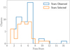 |
Fig. 2. Number of clusters that have a given number of observed spectroscopic targets (blue), and those considered in our analysis as bona fide red clump stars. |
2.4. The final sample
We plot in Fig. 3 the (X, Y) and (Z, RGC) distribution of the analyzed OCs. Our entire sample includes clusters preferentially in the first, second, and third Galactic quadrants. The clusters are confined to the thin disk, and only a few old clusters go beyond Z = 500 pc. Contrary to most of the samples where chemical clocks are analyzed, half of our sample is outside the 1 kpc local bubble around the Sun. In Fig. 4 we plot the color-magnitude diagram CMD of all clusters using the available memberships, with the retained RC stars. A table with a complete list of clusters including their ages, Galactic positions, number of stars observed, number of spectra and mean abundance results are provided in Table A.2.
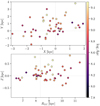 |
Fig. 3. Top: X,Y distribution of the sample of OCs used in this work, where the Galactic center is towards the right. Bottom: Z, RGC distribution of the sample of clusters. The color represents the age of the cluster. The dashed lines indicate the position of the Sun (X⊙, Y⊙, Z⊙) = (0, 0, 0), RGC = 8.34 kpc. |
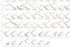 |
Fig. 4. Gaia DR2 color-magnitude diagrams of the sample of clusters used (sorted by age), retained RC targets are marked with a blue cross. The gray points correspond to the membership selections by Cantat-Gaudin et al. (2018); Gaia Collaboration (2018a). PARSEC isochrones (Marigo et al. 2017) of the corresponding metallicity computed in this paper are overplotted using distances provided by CG20, and ages and extinctions detailed in Sect. 4. |
Our sample includes five clusters that were discovered after Gaia DR2 (UBC clusters Castro-Ginard et al. 2020). This is the first time that chemical abundances are determined for them and the details will be provided in a separate paper (Casamiquela et al., in prep.)
The results of Teff and log g per star and cluster are shown in Fig. 5. The clusters are sorted by increasing age as determined in Sect. 4, and we overplot the corresponding isochrone of the [M/H] determined in this work to guide the eye. We see that in almost all clusters, the isochrone corresponds well to the parameters derived for the member RC stars. There are few cases where the retrieved atmospheric parameters are not fully in agreement with the expected RC traced by the isochrone. We do not find any relation between this disagreement and the age or any atmospheric parameter, but this is not uncommon for some stars at the low-S/N limit. We highlight the fact that King 1 is among the faintest clusters in the sample, has a mean [Fe/H] = 0.3, and its CMD in Fig. 4 shows that its membership selection can be uncertain. For the clusters where the mean of computed Teff and log g values are larger by at least 150 K or 0.2 dex with respect to the expected RC position of the model (Stock 1, NGC 6281, FSR 0850, NGC 2266, UBC 44, Melotte 72 and King 1), we keep an internal flag to discuss any possible effect that they may introduce in the abundance–age trends.
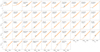 |
Fig. 5. Teff–log g diagrams resulting from the analysis of the analyzed RC stars in blue. The clusters are sorted according to age. The same isochrones of Fig. 4 are overplotted with the corresponding [M/H] and age. |
3. Differential chemical abundances
Our aim is to compute chemical abundances of 25 species in a line-by-line differential manner for all stars, with respect to a reference star. The set of lines to be used for the differential chemical abundance analysis were selected in the same way as in Paper I. In a first step, individual absolute chemical abundances per spectrum were obtained line-by-line using the atmospheric parameters fixed to the resulting values of Sect. 2.2. We used the same radiative transfer code (SPECTRUM), model atmospheres (MARCS), line list, and fitting algorithm as in Sect. 2.2. Hyperfine structure splitting and isotopic shifts were taken into account for the elements: V I, Mn I, Co I, Cu I, Ba II, La II, Pr II, and Nd II, following Heiter et al. (2015, 2021). Neither nonLTE nor 3D corrections were taken into account in the computation of the abundances. These corrections are in general small for nearly solar metallicity stars (Amarsi et al. 2020). In the case of this study, we have a narrow range of atmospheric parameters in our sample of stars and we performed a differential treatment of the abundances. This type of analysis helps to mitigate the possible departures from 1D/LTE, which are highly dependent on the lines used and the stellar parameter range. The differential abundance analysis provides high-precision abundance measurements, which erases most of the effects that introduce systematic uncertainties in the usual abundance computations (e.g., blends, incorrect atomic line parameters). To be able to apply this technique successfully, it is required that the sample of stars be in the same evolutionary stage as the reference star. A clear example of this is the analysis of solar twins with respect to the Sun, largely applied in the literature and usually using nearby solar twins (e.g., Meléndez et al. 2009; Tucci Maia et al. 2016) or solar analogs in clusters (e.g., Liu et al. 2016). Other works have applied the same strategy to other stellar types using a reference star very close to the sample of stars (e.g., Hawkins et al. 2016; Jofré et al. 2015; Blanco-Cuaresma & Fraix-Burnet 2018), as we did in Paper I.
All stars analyzed here are selected to match the RC position of the cluster, or be very close, as discussed in Sect. 2. However, the RC position slightly moves in the Kiel diagram as age and metallicity changes, which, in general, is reproduced by our Teff–log g results. Therefore, as the cluster sample spans a large range in age, stars do not have exactly the same atmospheric parameters, though are considered to be in the same evolutionary state. We consider the stars that are sufficiently similar to be able to apply this procedure. Additionally, for each cluster, we checked that the differences in the atmospheric parameters of the selected stars do not produce trends in abundances; for example, we checked for the existence of any dependence of abundances on Teff or log g (see e.g., Fig. A.3). The aim here is to minimize any possible bias in the abundances caused by differences in the atmospheric parameters of the selected stars.
3.1. Setting the reference values
As a reference star, we use the giant from the Hyades Gaia DR2 3312052249216467328 (gam Tau/HD 27371) also used as a reference in Paper I. From the analysis of two spectra of this star, we obtained mean atmospheric parameters Teff = 4975 ± 12 K, log g = 2.83 ± 0.03, and mean iron abundance [Fe/H] = 0.10 ± 0.05 (with respect to the Sun). The mean absolute difference between the full sample of stars and the reference star is 116 K and 0.21 dex in Teff and log g respectively, with the maximum difference being 460 K and 0.9 dex. These values are slightly larger than for the samples analyzed in Paper I, for the reasons mentioned above. We consider the sample of giants as analogs – close enough to the reference star – to safely perform this analysis. This is further justified because we do not find any remarkable trend of abundances with Teff or log g for the cluster stars with the largest range of atmospheric parameters.
The outcome is star-by-star element abundances computed with respect to the abundances of the reference star from the Hyades. Subsequently, we transformed the resulting abundances to a solar scale to be able to retrieve meaningful “bracket ratios” of abundances. To do so, we analyzed the solar analog from the Hyades Gaia DR2 3314109916508904064 (HD 28344; Teff = 5957 ± 32 K, log g = 4.49 ± 0.03, [Fe/H] = 0.12 ± 0.05) differentially with respect to the Sun using the same methodology. Considering the stars within the Hyades to have the same abundance pattern, we can transform the abundances of giants to the solar scale, adding to each element abundance the corresponding value of the solar analog of the Hyades.
3.2. Final cluster abundance
For each cluster, we performed a weighted mean to obtain the cluster mean abundance values, and we used the corresponding dispersion as uncertainties. The resulting cluster abundances are detailed in Table A.2. We plot in Fig. 6 the distribution of the retrieved [Fe/H] for all used stars, and the distribution of cluster ages as a function of mean [Fe/H] per cluster. The sample of clusters is constrained within the range of −0.2 < [Fe/H] < 0.2. Abundances with large uncertainties (> 0.2 dex, typically corresponding to the most uncertain elements or low-S/N spectra) are rejected and are not used in the computation of mean values because we do not consider them reliable for our purposes in this paper.
 |
Fig. 6. Top: distribution of solar scaled iron abundances of all analyzed stars. Bottom: distribution of cluster ages as a function of mean [Fe/H] (clusters with one measured star are plotted in orange). |
Figure 7 shows the mean [Fe/H] values per cluster retrieved here compared with the catalog of compiled cluster metallicities by Heiter et al. (2014). We have 23 clusters in common, and we find a generally good agreement (∼2σ) with literature values. There are differences in some cases, which are expected because of differences in the quality of the spectra and analysis pipelines. The most discrepant case is NGC 2266, with a difference of ∼0.6 dex, for which the literature value comes from one single star studied in Reddy et al. (2013)1. This star is not considered a member by Cantat-Gaudin et al. (2018), because its proper motions and parallax from Gaia DR2 differ with respect to the mean cluster values. Moreover, our determination for this cluster based on five members also points to a different radial velocity: we obtain a mean value of vr = 52 ± 2 km s−1 while the value found by Reddy et al. (2013) is −29.7 ± 0.2 km s−1. NGC 6791 presents a relatively large difference of 0.15 dex. It is the most metal-rich cluster in our sample, and therefore uncertainties and systematics in this study and/or the literature are possibly larger in this case.
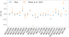 |
Fig. 7. Mean [Fe/H] values per cluster computed here (blue) compared with [M/H] literature values from Heiter et al. (2014) (orange) for the 23 clusters in common. |
We show the distribution of uncertainties in elemental abundances of individual stars (blue symbols), and of clusters with more than one measured star (orange symbols) in Fig. 8. To compute the cluster individual uncertainties, we used the standard deviation of the member abundances divided by  . Cluster uncertainties are in general much lower than the typical uncertainties of individual stars because of the good agreement among the different stars of the same cluster. We highlight that the most uncertain elements in our measurements are Zn, Zr, Mo, Ce, and Pr. For these elements, individual stars have typical uncertainties of > 0.1 dex. Cluster uncertainties are also found to be the largest for the same elements (∼0.05 dex), with long tails. These long tails are driven by a few clusters, typically: NGC 6791 and FSR 0850 have the largest uncertainties sometimes reaching 0.3 dex for Ce, Zn, and Mo.
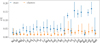 |
Fig. 8. Distribution of the uncertainties of abundances of the different elements: for the full sample of stars (blue), and the clusters with more than one measured star (orange). The median value is marked with a point, and the 16th and 84th percentiles are represented with the line. |
4. Ages
As a starting point for the cluster ages, we used the catalog of ages derived by CG20. That study obtained ages, extinctions, and distances for a large set of OCs from an artificial neural network using Gaia photometry and the mean parallax of the clusters. The algorithm was trained using a reference sample composed mainly by Bossini et al. (2019) (the largest homogeneous sample of cluster ages obtained from Gaia data), and was complemented with other smaller samples to allow coverage of older and more distant clusters. CG20 does not provide individual uncertainties per cluster, and therefore we assign age uncertainties extrapolated from Bossini et al. (2019). We took the median of Bossini et al. (2019) quoted uncertainties per age bin and used them as an estimation of the cluster uncertainty at a given age.
CG20 performed an external comparison of their set of ages, distances, and extinctions with large catalogs such as Kharchenko et al. (2013), finding good agreement on ages in general, with the exception of some young reddened objects. In the case of our clusters, the quoted ages, extinctions, and distance modulus are, in general, visually consistent in a CMD when using PARSEC isochrones. However, CG20 does not take into account the particularities of a given cluster, such as metallicity, to assign ages. From visual inspection of the Gaia CMDs, we spotted some cases where the quoted age can be adjusted when using an isochrone of the metallicity derived in Sect. 3. In these cases, we performed a manual refinement of the extinction and the age of the cluster, leaving the cluster mean distance constant because it is constrained mainly by the mean cluster parallax. We made the following changes (see Fig. 9):
 |
Fig. 9. Gaia DR2 CMDs (gray dots) of the clusters for which the ages and extinctions were refined with respect to the ones in CG20, as discussed in the main text. The orange isochrones are those with the values quoted in CG20, and the green ones are manually changed to adjust the shape of the main sequence, turnoff or red giant members. Target stars studied in this paper are marked with blue crosses. |
– King 1: The quoted age (3.89 Gyr) and extinction (1.89 mag) by CG20 seem to not fit the turnoff region of the cluster. For its super-solar metallicity of [Fe/H] = +0.3, a younger age of 2.8 Gyr and a larger absorption of 2 mag present a better fit. This age is in good agreement with previous dedicated studies of this cluster (2.8 ± 0.3 Gyr Carrera et al. 2017).
– NGC 6791: CG20 quotes an age of 6.76 Gyr and AV = 0.67 mag. This cluster also has a super-solar metallicity of [Fe/H] = +0.26. In this case, a decrease of the extinction to AV = 0.5 mag and an increase of the age to 8 Gyr provide a good fit of the turnoff, RGB, and red clump simultaneously. Again, in this case, the refined age is more compatible with other literature studies such as 7.7 ± 0.5 Gyr Grundahl et al. (2008) and ∼8 Gyr (Brogaard et al. 2012), both from different sets of isochrones.
– For the clusters FSR 0278 ([Fe/H] = +0.13) and NGC 2266 ([Fe/H] = +0.15) the quoted ages seem to nicely reproduce the shape in the CMD: 2.34 and 0.81 Gyr, respectively. However, a small change in the absorptions, which seems overestimated for both cases in CG20 (AV = 0.84, and AV = 0.25 mag, respectively), better fits the red clump and main sequence. We derive AV = 0.7 and 0.1 mag, respectively for the two clusters.
– The quoted values for NGC 1662 ([Fe/H] = −0.06) in CG20, 0.81 Gyr and AV = 0.42 mag, can be slightly refined to 0.7 Gyr and AV = 0.9 to fit better the turnoff and red giants.
– For NGC 6728 ([Fe/H] = 0.02) the quoted parameters in CG20 (620 Myr AV = 0.83) fit the turnoff and main sequence well, however the well-populated red clump is shifted upwards with respect to the isochrone. A smaller absorption of AV = 0.46 and older age of 750 Myr, similar to the one derived by Bostancı et al. (2018), produce a better fit to the clump, although this slightly compromises the fit to the main sequence.
– UBC 3 ([Fe/H] = −0.05) values from CG20 (140 Myr and AV = 0.9) can be slightly changed to 0.2 Gyr and AV = 1.2 mag to provide a more adequate fit of the main sequence and red clump.
The ages of our analyzed clusters range between 140 Myr and 7 Gyr, most of them having ages < 3 Gyr.
5. Chemical trends of [X/Fe] with age
We plot the [X/Fe]2 of all the measured chemical elements as a function of the log age of clusters in Fig. 10. We mark the clusters closer than 1 kpc in orange. For clarity, we only plot those clusters for which uncertainties in abundance are lower than 0.15 dex in the specific element. We highlight in red circles the flagged clusters in Sect. 2.4. A complementary figure with [X/Fe] as a function of [Fe/H] and colored by age can be found in Fig. A.4.
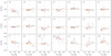 |
Fig. 10. [X/Fe] abundances of all measured elements as a function of age in logarithmic scale. Clusters located at less than 1 kpc from the Sun are plotted in orange. Uncertainties in the x coordinate are smaller than the points. Red circles correspond to the clusters with stars with more uncertain atmospheric parameters. |
Most of the ratios from Na to Ni exhibit a mostly flat behavior as a function of age, which is expected in the metallicity range of the clusters (see Kobayashi et al. 2020). However, some of them seem to have a mild increasing trend starting at 1 Gyr (Al, Si, V, Mn, Co, Ni). We remark that Na, Cu, and Mn have the largest spreads in these spaces, and a small negative zero point. This could be due to nonLTE effects (Yan et al. 2016; Bergemann et al. 2019), which usually depend on the atmospheric parameters of the stars, and are not taken into account when doing the transformation from differential abundances with respect to giants to solar-scaled abundances. In several elements (e.g., Mg, Si), the flagged clusters in red tend to be slightly off from the distribution of the other clusters, showing that they probably carry larger uncertainties. Zn also shows a negative zeropoint of the abundances relative to Fe of around −0.2 dex. A similar zeropoint was found by Duffau et al. (2017), who studied Zn abundances with Gaia-ESO survey data for field giants at solar metallicity. These authors concluded that this cannot be explained by systematic uncertainties such as nonLTE or 3D effects, and attributed the underabundances to a real signature of chemical enrichment. After studying this effect as a function of Galactocentric radius, metallicity, and age, the authors tentatively explained it as being due to dilution from almost Zn-free Type 1a supernova ejecta.
The s-process elements (Y, Zr, Mo, Ba, Ce, Pr, Nd) are plotted in the third row in Fig. 10. In general, we observe a change of behavior for all these elements at 1 Gyr, traced with less dispersion for the nearby clusters. This is particularly remarkable for Y, Zr, Mo, Ba, Ce, and Nd. These elements exhibit a sort of plateau with large scatter at ages younger than ∼1 Gyr, but at different “saturation” values, with Ba being the largest one. Older than 1 Gyr, the abundances show a significant negative trend with age. Some of the elements exhibit large dispersion, such as Mo, which makes the decreasing trend less clear. Praseodymium shows the opposite trend, with increasing values as a function of age. Furthermore, this element has a significant contribution to the r-process (see more details in Sect. 6), which could cause this remarkably different behavior.
Barium is the s-process element that shows the largest [X/Fe] abundances for young OCs, which diminishes significantly at older ages (∼2 Gyr), approaching solar values. This is a known phenomenon without a satisfactory explanation, and has been investigated by other authors before (e.g., D’Orazi et al. 2009; Mishenina et al. 2013; Magrini et al. 2018) with smaller samples of OCs. For the first time, D’Orazi et al. (2009) showed a sharp decreasing trend of [Ba/Fe] in a sample of 20 clusters, which could be explained using chemical evolution models with enhanced yields of the s-process production by AGB stars below 1.5M⊙. Some samples of field stars, for example that of Bensby et al. (2005), also show that young stars seem Ba-enhanced, even though their sample is limited to slightly older ages than the OCs, and exhibits a much larger spread in [Ba/Fe]. This is possibly because the ages of field stars computed by isochrone fits are much less accurate than the ages of clusters. Maiorca et al. (2011) used a similar sample of OCs to that of D’Orazi et al. (2009) and computed other s-process elements (Y, Zr, La and Ce) to also find decreasing dependencies. For these four elements, these latter authors spotted a plateau at ages younger than ∼1 Gyr, but this was not seen for Ba. Later, Jacobson & Friel (2013) argued that not all s-process elements follow this decreasing trend, for example Zr and La showed different trends. More recently, Magrini et al. (2018) analyzed s-process elements (Y, Zr, Ba, La, Ce, Eu) in a sample of 22 clusters in the Gaia-ESO survey, and found steep trends in Y, Zr, and Ba and lower correlations for La and Ce. These authors attribute this to the lower number of stars measured for these elements. Special caution needs to be taken when interpreting Ba results because several studies recently suggested that Ba II lines are influenced by several effects in young stars. For instance, Reddy & Lambert (2017) found a strong correlation between stellar activity and Ba II abundance obtained from the 5853 Å line, which forms in the upper layers of the stellar photosphere where the effects of the active chromosphere are strong for young stars (t < 150 Myr). Here, we are also using the line at 6141 Å, which gives very consistent abundances with the line at 5853 Å with our sample of red clump stars. Moreover, nonLTE effects could be important in this range of metallicity for Ba II lines (Mashonkina et al. 1999; D’Orazi et al. 2009).
Here we see clear decreasing trends of all s-process elements (except Pr), with a sort of plateau at young ages. Thus, our results are in line with those of previous studies by Magrini et al. (2018), Maiorca et al. (2011), but with more than double the number of clusters, and overall lower uncertainties in the measured abundances. We find that Ba is the element that reaches the largest value in this plateau, namely ∼0.4 dex. Lower values are found for Ce, Y, and Nd (∼0.15 dex), and Mo and Zr (∼0 dex). Supersolar values of these abundances were also found very recently by Spina et al. (2021), who used the GALAH DR3 survey data. However, no clear trends with age are seen in their sample, probably because of the smaller number of clusters with measured neutron-capture elements.
The spatial coverage of our sample goes beyond the solar neighborhood with a range of 6 < RGC < 11 kpc (see Fig. 3). Figure 10 allows us to distinguish between the clusters inside a 1 kpc bubble around the Sun (orange) and those outside (blue). Both subsets have similar age and metallicity distributions, though the > 1 kpc sample is dominated by clusters in the outer disk, which also tend to be more scattered in the Z coordinate (Fig. 3). Magrini et al. (2018) also carried out a spatial analysis, comparing clusters from the solar neighborhood to those in the inner disk, concluding that, focusing on the young age range (< 1 − 2 Gyr), solar neighborhood OCs (6.5 < RGC < 9.5) have higher [X/Fe] than those in the inner disk (RGC < 6). We do not observe this behavior; we see that the trends of the s-process elements are qualitatively satisfied in all distance regimes. However, our distance range is more limited than that of Magrini et al. (2018) in the inner disk.
6. Chemical clocks
Several combinations of elements produced by different stellar progenitors, and thus produced at different timescales, have proven to be useful for deriving empirical ages (see e.g., discussion in Nissen 2015). This is already seen in Fig. 10, where some [X/Fe] have steep trends with age, and others are flat (see also extended discussion by Delgado Mena et al. 2019).
Nissen (2015) and Spina et al. (2018), among several other authors, analyzed the tight linear dependence of [Y/Mg] and [Y/Al] as a function of age with solar twins. Both are promising chemical clocks, and are presumably useful for retrieving ages up to a precision of ∼0.5 Gyr in a limited range of metallicities (Feltzing et al. 2017). This is expected taking into account the timescale of formation of those elements, because nearly all odd-Z and α elements are synthesized by core-collapse supernovae (Woosley et al. 2002; Kobayashi et al. 2020), contrary to most s-process elements whose production is dominated by intermediate-mass stars in their AGB phase.
Some further studies (Jofré et al. 2020; Delgado Mena et al. 2019) found other possibilities of combinations of elements useful as chemical-clock candidates. A linear regression as a function of stellar age is able to retrieve some abundance ratios with slopes as significant as that of [Y/Mg] determined by Nissen (2015), for example. However, as pointed out by Delgado Mena et al. (2019), some of these ratios might hold only for certain ranges of metallicity.
6.1. The solar neighborhood
In this section, we use our sample of clusters to investigate all possible combinations of elements that show a significant correlation with age. We plot our results as a function of age in a linear scale (instead of logarithmic scale as in Sect. 5) so that we can quantitatively compare our linear fits to those performed in the literature. We only use the subsample of clusters inside the 1 kpc bubble in order to reproduce similar conditions as in previous studies that investigate chemical clocks. None of the five flagged clusters in Sect. 2.4 are in this subsample.
In general, we expect a trend when the timescales of production of the two elements involved differ (in particular, when the slopes of the trend found for the two elements as a function of age in Fig. 10 go in opposite directions). We used the Bayesian outlier rejection algorithm explained in detail in Hogg et al. (2010)3 to perform a linear fit with uncertainties to the different combinations of abundances. This algorithm is suitable in our case because our data are scarce, and helps to retrieve more robust estimates and uncertainties of the fitted parameters. The algorithm infers at the same time the two parameters of the fit together with a distribution of outliers. The model is run 15 000 times through a Markov chain Monte Carlo (MCMC), and the best values of the slope and intercept are taken as the maximum of the posterior. We selected those for which we obtain slopes more significant than 3σ, with absolute values ≥0.04 dex Gyr−1, and errors smaller than 0.03 dex Gyr−1. We find 19 significant combinations within our sample (including [Y/Mg] and [Y/Al]), as plotted in Fig. 11. In each panel, we indicate the value of the slope with its uncertainty. In addition, following Jofré et al. (2020), we color-code each element by nucleosynthetic family in order to guide the eye and aid interpretation. Similarly to Jofré et al. (2020), we find that all selected ratios involve at least one element produced partially by the s-process. Y, Zr, and Ba have a large contribution from the s-process (more than ∼60% Bisterzo et al. 2014), because these are mainly produced by intermediate-mass stars in their AGB phase, and therefore these elements are ejected to enrich the interstellar medium on an overall large timescale. The r-process, on the contrary, is believed to happen in core-collapse supernovae and possibly other more exotic places like neutron star mergers (Thielemann et al. 2017), where a large density of neutrons is available. Neodymium has a significant contribution from the r-process.
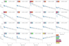 |
Fig. 11. Abundance ratios for which a significant level of correlation is found. Only clusters closer than 1 kpc and with more than one star are plotted. Error bars for the x-axis are usually smaller than the point size. The best-fit model is overplotted in black (the resulting slope written in each panel in dex Gyr−1), and the light gray lines correspond to the sampling of the MCMC. Element names are colored depending on the chemical family they belong to. |
We find that the “purest” s-process elements (Y, Zr and Ba) produce significant correlations when combined with α-elements, particularly with Mg, Si, Ca, and Ti. Only Y has a significant correlation with Al. In these combinations, Ba is the element for which we find the steepest slopes, which are always close to −0.1 dex Gyr−1. We remind the reader that Ba abundances can be affected by activity and nonLTE effects as discussed in Sect. 5. Both Y and Zr typically show smaller slopes, except for the combination with Al (and some Fe-peak elements) which gives −0.07 dex Gyr−1. The different behavior of s-process elements may reflect how differently their production evolves with time. In general, our slopes have higher values with respect to Jofré et al. (2020), especially those involving Ba since our values are close to −0.10 dex Gyr−1, whereas Jofré et al. (2020) obtain values of around −0.04 dex Gyr−1. This is a reflection of the steeper [Ba/Fe] trend in Fig. 10 seen in clusters and also in other studies (discussed in detail in Sect. 5), in comparison with field stars. We note that in the Ba relations there are persistently three outliers that are usually detected by our algorithm: the Hyades cluster, NGC 2632, and NGC 6997.
Neodymium is a heavy neutron-capture element with a significant contribution from both the s-process and the r-process, around 50% of each path. We find positive slopes of Nd when combined with the s-process element Zr (also produces a similar correlation with Ba but it does not get selected because of low significance). The sign of the slope goes in the opposite direction, indicating that its production timescale is much shorter than that of Zr. This is also related to the different slope of the [Nd/Fe] versus age from that of [Zr/Fe], as seen in Fig. 10.
We also find that Y has trends with almost all Fe-peak elements. Again, this is explained in Fig. 10: a steep trend from Y which produces a slope when combined with the flat trend of Fe-peak elements. From the other s-process elements, only Ba produces a trend with Sc, and Mo with Zn. All Fe-peak elements have significant contributions from both core-collapse supernovae and type Ia supernovae, with slightly different yields depending on the element, except for Cu and Zn which are almost entirely produced by core-collapse supernovae, but with yields depending on metallicity. This makes it difficult to interpret our obtained trends in this family of elements. This result is not new: Jofré et al. (2020) also found some significant trends with the iron-peak element family, particularly Ni, Mn, and Co when combined with s-process elements.
We want to highlight that some of the trends can be very sensitive to the nonuniform distribution in the age of our (and any) sample of clusters, biased towards young ages, and thus very dependent on the abundances of the few old clusters. Even though our sample is the largest of the clusters used to study age–abundance relations, some of our trends carry large uncertainties because of the low number of clusters. Additionally, beyond pure nucleosynthetic arguments, the trends must also be interpreted whilst taking into consideration the high complexity in the chemical substructures in the local chemical abundance space, as shown for example by Anders et al. (2018). In the same spatial volume, one can find several subgroups of stars belonging to different populations, including inner disk and outer disk migrators, stars in eccentric orbits, and so on. This effect gets more important when the volume analyzed increases, like in the present work compared to the previous samples of solar analogs. Thus, the difference in the slopes found and in the scatter of abundance at a given age with respect to those found by Jofré et al. (2020) have to be interpreted in the context of a chemo-dynamical picture of the Galaxy. This is discussed in the following section.
6.1.1. [Y/Mg] and [Y/Al].
The two most studied chemical clocks in the literature are [Y/Mg] and [Y/Al]. Figure 11 shows that they exhibit significant trends with age when we use the sample of clusters in the local bubble. This indicates that red giants also verify the age dependence of these two ratios, as seen in the literature with solar-type stars. Here we aim to quantitatively compare our results with the trends traced by solar twins for these two ratios of abundances (Nissen 2015; Spina et al. 2018).
The top panels of Fig. 12 show the obtained abundances of [Y/Mg] (left) and [Y/Al] (right) versus the age of the clusters closer than 1 kpc with at least two members with measured abundances, which we consider to have more reliable uncertainties (given by the dispersion of the star-by-star abundances). This is the same sample as the one used in Fig. 11, and the corresponding linear fit obtained is:
![$$ \begin{aligned} \mathrm{[Y/Mg]}&= 0.198\,(\pm 0.014) - 0.055\,(\pm 0.007)\cdot \mathrm{Age} \nonumber \\ \mathrm{[Y/Al]}&= 0.200\,(\pm 0.013) - 0.070\,(\pm 0.007)\cdot \mathrm{Age} . \end{aligned} $$](/articles/aa/full_html/2021/08/aa39951-20/aa39951-20-eq2.gif)
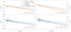 |
Fig. 12. [Y/Mg] (left) and [Y/Al] (right) abundances of our sample of clusters (with more than one measured star) as a function of age. In the top panel we plot the clusters closer than 1 kpc (orange), and in the bottom panel clusters at all distances. The clusters marked with red circles are those flagged in Sect. 2.4. The linear fits done for the close (all) clusters are plotted in orange (blue) lines, accounting for uncertainties. The values of the obtained slopes are indicated. The results of the linear fit performed by Spina et al. (2018) are shown in black for comparison purposes. |
The linear fit of the decreasing trend with age obtained by Spina et al. (2018) is overplotted in black which corresponds to the slopes of −0.046 ± 0.002 dex Gyr−1 for [Y/Mg] and −0.051 ± 0.002 dex Gyr−1 for [Y/Al]. These values of the slopes are also similar to those found in other studies Nissen (e.g. 2015, 2016), although our values have larger uncertainties compared to the analyses done with solar twins. This is probably due to the smaller number of clusters. We plot in red the only flagged cluster in Sect. 2.4 closer than 1 kpc and with more than 1 star, namely NGC 6181. The best-fit result does not change if we do not take into account this cluster. The [Y/Al] slope is only compatible at ∼2σ with that of Spina et al. (2018), and additionally, we find a zero point of ∼0.05 dex in the [Y/Al] abundance compared to them. Some studies using stars of different spectral types in clusters (e.g., Souto et al. 2018) show that diffusion affects the abundances of some elements – such as Al – of main sequence stars, with differences as high as 0.1 dex. Later in stellar evolution, in the RGB, the convective envelopes tend to restore initial chemical abundances. Thus, it could be that diffusion is affecting the abundances of the studies in the literature. The offset could also be explained if Al suffers from nonLTE effects in giants (Andrievsky et al. 2008), which we do not take into account in this work. It could also be related to the fact that some light elements can be affected by internal mixing processes in giants, which alter the relations between age and abundance and can be significant for Al (Smiljanic et al. 2016). This issue needs further investigation. This may mean that the [Y/Al] relations obtained with dwarfs give biased results when used to obtain the ages of giants, or vice versa.
6.2. Beyond the local bubble
Here, we want to investigate the spatial dependence of chemical clocks, and in particularly to decipher whether or not the inclusion of distant OCs significantly changes the locally derived slopes. The bottom panels of Fig. 12 show the obtained abundances of [Y/Mg] (left) and [Y/Al] (right) versus age of all clusters analyzed in this paper. The corresponding linear fit is also plotted, and was performed in the same way as for the clusters in the solar neighborhood. We notice a remarkably greater dispersion when compared to the results of the local bubble or to the studies of solar twins in the literature. The results of these fits are:
![$$ \begin{aligned} \mathrm{[Y/Mg]}&= 0.199\,(\pm 0.017) -0.055\,(\pm 0.011)\cdot \mathrm{Age} \nonumber \\ \mathrm{[Y/Al]}&= 0.182\,(\pm 0.012) - 0.061\,(\pm 0.005)\cdot \mathrm{Age} . \end{aligned} $$](/articles/aa/full_html/2021/08/aa39951-20/aa39951-20-eq3.gif)
The two sets of slopes (Eqs. (1) and (2)) are compatible within 1σ, though in [Y/Al] we obtain slightly flatter slopes when using the full sample compared to the close one. This last conclusion needs to be taken with caution, because the samples are small in numbers, and our fits carry large uncertainties. Nevertheless, in Fig. 12 we see a significantly larger scatter in abundances of the distant clusters compared to close ones. We interpret this as a hint that the abundance–age relations may be dependent on the spatial volume analyzed. Assuming that possibly the samples of stars get mixed due to dynamical processes of the Milky Way, enlarging the analyzed volume introduces more scatter in these relations. Performing the fit with or without the flagged clusters (marked in red in Fig. 12; see Sect. 2.4) retrieves very similar slopes: −0.054 ± 0.007 and −0.064 ± 0.005 dex Gyr−1, for [Y/Mg] and [Y/Al].
Figure 13 shows the residuals4 of the [Y/Mg] versus age of the sample of clusters separated in bins of RGC: inner disk (RGC ≤ 8 kpc), solar neighborhood (8 < RGC < 9 kpc), and outer disk (RGC ≥ 9 kpc). By doing a weighted standard deviation of the residuals in these three ranges, we obtain larger dispersions in the inner and outer disk of 0.07 and 0.14 dex, respectively, in comparison with the solar radius which is 0.04 dex. The most discrepant clusters tend to be young (∼500 Myr) in both the inner and outer samples. These clusters also tend to have large uncertainties in our [Y/Mg] abundances (∼0.1 dex). However, we notice in the plot that there are cases where the uncertainties in the [Y/Mg] determination are small, but provide large residuals. This is the case for the cluster NGC 6705 (M 11, Age = 300 Myr), which gives a difference in abundance of 0.12 dex with an uncertainty of δ[Y/Mg] = 0.04 based on 12 members. This cluster is nevertheless peculiar for its α-enhancement (Casamiquela et al. 2018).
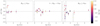 |
Fig. 13. Residuals in the [Y/Mg] (with respect to the linear fit for the closest sample Eq. (1)) versus age in three bins of Galactocentric radius, indicated in each panel. The color code is the derived [Fe/H] abundance. |
We do not see a clear dependence of the residuals on metallicity or height above the Galactic plane. However, we note that clusters in the outer disk tend to be more scattered vertically (as can be seen in Fig. 3).
Translating abundance scatter into age scatter, we obtain that the [Y/Mg] relations, even inside the ∼1 kpc bubble around the Sun, could predict ages with a precision of ∼1 Gyr at best. This result goes is in line with the recent findings of Morel et al. (2021), who investigated several age–abundance relations using 13 stars in the Kepler field with asteroseismic ages. These authors find that the seismic and abundance-based ages differ on average by ∼1.5 Gyr and attribute this to a variety of factors, including the presence of small zero-point offsets between chemical abundances and those used to construct the age–abundance calibrations.
A similar experiment was done in the recent work by Casali et al. (2020). The authors noticed that ages computed from [Y/Mg] of a subsample of OCs towards the inner disk (RGC < 7 kpc) were in general overestimated with respect to literature (isochrone) ages. This sample of clusters in the inner Galaxy is, in general, more metal-rich than the rest of their sample ([Fe/H] ≳ 0.2 dex), and the differences they obtain in age are between 2 and 8 Gyr. The authors attribute these large discrepancies to the fact that the yields of s-process elements have a nonmonotonic dependence on metallicity. This metallicity dependence is particularly important for heavy elements, which are secondary elements produced depending on the number of seeds available (iron-peak elements). In our sample, we do not see a striking dependence of the residuals on metallicity. This could be because our metallicity range is slightly narrower than theirs, and in particular we have fewer metal-rich clusters.
We have eight clusters in the inner RGC range (RGC ≤ 8 kpc), and the clusters NGC 6645 and NGC 6705 are the discrepant ones. Otherwise, the scatter of the residuals of the other clusters is 0.01 dex. On the contrary, we observe a larger offset and dispersion towards the outer Galaxy (RGC ≥ 9 kpc) based on 16 clusters. Some studies have argued that OCs undergo radial mixing processes to the same degree as single field stars (Casamiquela et al. 2017). Therefore, an interpretation of the large scatter in the abundances of clusters is that when sampling beyond the very local solar neighborhood traced by solar twins (typically confined within ∼100 pc around the Sun) there is a higher chance of including stars and clusters that have migrated radially from their birthplaces and therefore trace a different chemical enrichment history. Thus, simple abundance–age relations would no longer be valid because of the complexity introduced by the dynamical processes.
7. Conclusions
Clusters are good complements to solar twins for investigating trends of chemical abundance ratios with age. Their ages can be estimated with high precision through their color–magnitude diagrams together with Gaia parallaxes, and therefore they allow us to probe outside the local bubble.
We homogeneously analyzed high-resolution spectra from 209 red clump stars in 47 OCs ranging ages between 140 Myr and 7 Gyr and metallicities between −0.2 and 0.2 dex. We derive atmospheric parameters with typical uncertainties of 18 K in Teff and 0.045 dex in log g. We retrieve abundances of 25 chemical species using a line-by-line technique using spectral synthesis fitting for all stars with respect to a giant in the Hyades cluster. We transformed these to solar-scaled abundances using a solar analog of the Hyades analyzed with respect to the Sun. This proves to be a useful way to retrieve high-precision abundances of stars of different spectral types inside a cluster, without the need to observe solar twins, which are fainter. We retrieve cluster mean abundances with a typical scatter of 0.02 dex in most of the elements, except for heavy elements, for which dispersions are larger.
We analyzed the behavior of [X/Fe] abundances with log Age. Elements from Na to Zn generally exhibit flat trends, with large scatter in Mn, Cu, and Zn, and remarkable zero points in Na, Mn, and Zn. We find a knee in most neutron-capture elements at around 1 Gyr, followed by a decreasing trend of abundance with log Age, particularly in Ba, Ce, Y, Nd, Zr, and Mo. The mentioned elements exhibit a plateau at young ages (< 1 Gyr) with different values (Ba being the largest one at ∼0.4 dex).
Using the sample of clusters inside a 1 kpc bubble around the Sun, we find 19 different [X1/X2] combinations that have strong correlations with age in our metallicity range, particularly those that involve elements produced via the s-process. We find that Y, Zr, and Ba (which have a large contribution to the s-process) always produce correlations when combined with α-elements. Among all significant combinations, we find the largest slopes for those with Ba, such as [Ba/Mg] (0.098 ± 0.035 dex Gyr−1). However, we highlight that according to the literature, Ba II lines can be affected by activity in young stars, and on top of this NLTE corrections may be needed. We compare some of the slopes with those derived by Jofré et al. (2020), and we find that in general, our slopes are steeper. Special caution needs to be taken in this type of comparison because the age distribution of our (and any) sample of clusters is biased towards young ages, and therefore slopes are very sensitive to the values of old clusters. The discovery of new clusters in our Galaxy thanks to Gaia is going to improve this situation and help future studies in this direction.
A linear fit to [Y/Mg] and [Y/Al] versus cluster age retrieves similar slopes to those already published in the literature: −0.055 ± 0.007 dex Gyr−1 and −0.070 ± 0.007 dex Gyr−1, respectively. Our [Y/Al] trend differs in slope with respect to the findings of other authors, and shows an overall offset in abundances which may be related to NLTE effects or mixing in giants, or alternatively to diffusion in main sequence stars used for the literature studies. This needs to be further assessed before using this clock to date stars. The differences found also point towards some difficulties in computing ages using chemistry alone.
We investigate the validity of the abundance–age relations outside the local bubble. In [Y/Al] we obtain a slightly flatter slope when using the full sample of clusters, though this is not the case with [Y/Mg]. In both ratios, we see a larger scatter introduced. We interpret this as a hint that the chemical clocks may not be as universal as previously thought, but instead they probably have a dependence on the spatial volume analyzed. The residuals of the [Y/Mg] fit have values around 0.04 dex for the clusters in the solar radius (8 < RGC < 9 kpc). For the outer Galaxy (RGC ≥ 9 kpc), the comparison of abundances of the 16 clusters seems to disagree more, with a scatter of 0.14 dex in the residuals. We show that these differences are not fully explained by uncertainties in the [Y/Mg] value. This scatter translates into an age precision of 1 Gyr at best.
Thanks to the spatial coverage of our sample of clusters, our results point to a nonuniversality of the abundance–age relations, in the sense that expanding the spatial volume analyzed may increase the chance of including migrators which will certainly trace a different enrichment history. Thus, one needs to understand the abundance trends also in terms of the complexity of the chemical space introduced by the Galactic dynamics, on top of pure nucleosynthetic arguments (e.g., Anders et al. 2018). Particular caution needs to be taken when trying to apply these relations to date samples of stars located beyond the local bubble.
Our code is adapted from the one available in https://www.astroml.org/book_figures/chapter8/fig_outlier_rejection.html, which uses the python library PyMC3.
With respect to the linear fit done for the sample of close clusters: Eq. (1).
Acknowledgments
We thank the anonymous referee for the useful comments which helped to improve the quality and results of the paper. This work has made use of data from the European Space Agency (ESA) mission Gaia (http://www.cosmos.esa.int/gaia), processed by the Gaia Data Processing and Analysis Consortium (DPAC, http://www.cosmos.esa.int/web/gaia/dpac/consortium). We acknowledge the Gaia Project Scientist Support Team and the Gaia DPAC. Funding for the DPAC has been provided by national institutions, in particular, the institutions participating in the Gaia Multilateral Agreement. This research made extensive use of the SIMBAD database, and the VizieR catalogue access tool operated at the CDS, Strasbourg, France, and of NASA Astrophysics Data System Bibliographic Services. We also thank the staff for maintaining the public archives of ready-to-use spectra at ESO, NOT, OHP, CFHT and TBL. This work has used data from the ESO programs: 091.C-0438(A), 079.C-0131(A), 075.C-0140(A), 077.C-0364(E),076.C-0429(A), 0101.C-0274(A), 0104.C-0358(A),0102.C-0812(A), 092.C-0282(A), 076.B-0055(A), 60.A-9036(A),094.C-0297(A), 095.C-0367(A), 383.C-0170(A), 080.C-0071(A),081.C-0119(A), 082.C-0333(A), 083.C-0413(A), 079.C-0329(A),099.C-0304(A), 0100.C-0888(A), 266.D-5655(A),185.D-0056(C), 193.B-0936(D), 185.D-0056(I), 70.D-0421(A),088.C-0513(B), 094.D-0596(A), 086.C-0145(A), 380.C-0083(A), 097.A-9022(A), 085.D-0093(A), 072.C-0393(D),0100.A-9018(A), 083.A-9011(A) L.C., C.S., Y.T. and N.L. acknowledge support from “programme national de physique stellaire” (PNPS) and from the “programme national cosmologie et galaxies” (PNCG) of CNRS/INSU. We acknowledge the support of the scientific cooperation program ECOS-ANID Number 180049. L.C. acknowledges the support of the postdoc fellowship from French Centre National d’Etudes Spatiales (CNES). P.J. acknowledges financial support of FONDECYT Iniciación grant Number 11170174 and FONDECYT Regular grant Number 1200703. This work was partially supported by the Spanish Ministry of Science, Innovation and University (MICIU/FEDER, UE) through grant RTI2018-095076-B-C21, and the Institute of Cosmos Sciences University of Barcelona (ICCUB, Unidad de Excelencia ‘María de Maeztu’) through grant CEX2019-000918-M.
References
- Amarsi, A. M., Lind, K., Osorio, Y., et al. 2020, A&A, 642, A62 [EDP Sciences] [Google Scholar]
- Anders, F., Chiappini, C., Santiago, B. X., et al. 2018, A&A, 619, A125 [NASA ADS] [CrossRef] [EDP Sciences] [Google Scholar]
- Andrievsky, S. M., Spite, M., Korotin, S. A., et al. 2008, A&A, 481, 481 [NASA ADS] [CrossRef] [EDP Sciences] [Google Scholar]
- Bensby, T., Feltzing, S., Lundström, I., & Ilyin, I. 2005, A&A, 433, 185 [NASA ADS] [CrossRef] [EDP Sciences] [Google Scholar]
- Bergemann, M., Gallagher, A. J., Eitner, P., et al. 2019, A&A, 631, A80 [NASA ADS] [CrossRef] [EDP Sciences] [Google Scholar]
- Bisterzo, S., Travaglio, C., Gallino, R., Wiescher, M., & Käppeler, F. 2014, ApJ, 787, 10 [NASA ADS] [CrossRef] [Google Scholar]
- Blanco-Cuaresma, S. 2019, MNRAS, 486, 2075 [Google Scholar]
- Blanco-Cuaresma, S., & Fraix-Burnet, D. 2018, A&A, 618, A65 [NASA ADS] [CrossRef] [EDP Sciences] [Google Scholar]
- Blanco-Cuaresma, S., Soubiran, C., Heiter, U., & Jofré, P. 2014, A&A, 569, A111 [NASA ADS] [CrossRef] [EDP Sciences] [Google Scholar]
- Bossini, D., Vallenari, A., Bragaglia, A., et al. 2019, A&A, 623, A108 [NASA ADS] [CrossRef] [EDP Sciences] [Google Scholar]
- Bostancı, Z. F., Yontan, T., Bilir, S., et al. 2018, Ap&SS, 363, 143 [CrossRef] [Google Scholar]
- Brogaard, K., VandenBerg, D. A., Bruntt, H., et al. 2012, A&A, 543, A106 [NASA ADS] [CrossRef] [EDP Sciences] [Google Scholar]
- Cantat-Gaudin, T., Jordi, C., Vallenari, A., et al. 2018, A&A, 618, A93 [NASA ADS] [CrossRef] [EDP Sciences] [Google Scholar]
- Cantat-Gaudin, T., Anders, F., Castro-Ginard, A., et al. 2020, A&A, 640, A1 [NASA ADS] [CrossRef] [EDP Sciences] [Google Scholar]
- Carrera, R., Rodríguez Espinosa, L., Casamiquela, L., et al. 2017, MNRAS, 470, 4285 [NASA ADS] [CrossRef] [Google Scholar]
- Casali, G., Spina, L., Magrini, L., et al. 2020, A&A, 639, A127 [CrossRef] [EDP Sciences] [Google Scholar]
- Casamiquela, L., Carrera, R., Jordi, C., et al. 2016, MNRAS, 458, 3150 [NASA ADS] [CrossRef] [Google Scholar]
- Casamiquela, L., Carrera, R., Blanco-Cuaresma, S., et al. 2017, MNRAS, 470, 4363 [NASA ADS] [CrossRef] [Google Scholar]
- Casamiquela, L., Carrera, R., Balaguer-Núñez, L., et al. 2018, A&A, 610, A66 [NASA ADS] [CrossRef] [EDP Sciences] [Google Scholar]
- Casamiquela, L., Blanco-Cuaresma, S., Carrera, R., et al. 2019, MNRAS, 490, 1821 [NASA ADS] [CrossRef] [Google Scholar]
- Casamiquela, L., Tarricq, Y., Soubiran, C., et al. 2020, A&A, 635, A8 [NASA ADS] [CrossRef] [EDP Sciences] [Google Scholar]
- Castro-Ginard, A., Jordi, C., Luri, X., et al. 2018, A&A, 618, A59 [NASA ADS] [CrossRef] [EDP Sciences] [Google Scholar]
- Castro-Ginard, A., Jordi, C., Luri, X., Cantat-Gaudin, T., & Balaguer-Núñez, L. 2019, A&A, 627, A35 [NASA ADS] [CrossRef] [EDP Sciences] [Google Scholar]
- Castro-Ginard, A., Jordi, C., Luri, X., et al. 2020, A&A, 635, A45 [NASA ADS] [CrossRef] [EDP Sciences] [Google Scholar]
- Charbonnel, C., Lagarde, N., Jasniewicz, G., et al. 2020, A&A, 633, A34 [CrossRef] [EDP Sciences] [Google Scholar]
- Chiappini, C., Anders, F., Rodrigues, T. S., et al. 2015, A&A, 576, L12 [NASA ADS] [CrossRef] [EDP Sciences] [Google Scholar]
- da Silva, R., Porto de Mello, G. F., Milone, A. C., et al. 2012, A&A, 542, A84 [NASA ADS] [CrossRef] [EDP Sciences] [Google Scholar]
- Delgado Mena, E., Moya, A., Adibekyan, V., et al. 2019, A&A, 624, A78 [NASA ADS] [CrossRef] [EDP Sciences] [Google Scholar]
- Donor, J., Frinchaboy, P. M., Cunha, K., et al. 2018, AJ, 156, 142 [NASA ADS] [CrossRef] [Google Scholar]
- D’Orazi, V., Magrini, L., Randich, S., et al. 2009, ApJ, 693, L31 [NASA ADS] [CrossRef] [Google Scholar]
- Duffau, S., Caffau, E., Sbordone, L., et al. 2017, A&A, 604, A128 [NASA ADS] [CrossRef] [EDP Sciences] [Google Scholar]
- Feltzing, S., Howes, L. M., McMillan, P. J., & Stonkutė, E. 2017, MNRAS, 465, L109 [Google Scholar]
- Freeman, K., & Bland-Hawthorn, J. 2002, ARA&A, 40, 487 [Google Scholar]
- Friel, E. D. 2013, Open Clusters and Their Role in the Galaxy, eds. T. D. Oswalt, & G. Gilmore, 347 [Google Scholar]
- Gaia Collaboration (Babusiaux, C., et al.) 2018a, A&A, 616, A10 [NASA ADS] [CrossRef] [EDP Sciences] [Google Scholar]
- Gaia Collaboration (Brown, A. G. A., et al.) 2018b, A&A, 616, A1 [NASA ADS] [CrossRef] [EDP Sciences] [Google Scholar]
- Gray, R. O., & Corbally, C. J. 1994, AJ, 107, 742 [Google Scholar]
- Grundahl, F., Clausen, J. V., Hardis, S., & Frandsen, S. 2008, A&A, 492, 171 [NASA ADS] [CrossRef] [EDP Sciences] [Google Scholar]
- Gustafsson, B., Edvardsson, B., Eriksson, K., et al. 2008, A&A, 486, 951 [NASA ADS] [CrossRef] [EDP Sciences] [Google Scholar]
- Hawkins, K., Masseron, T., Jofré, P., et al. 2016, A&A, 594, A43 [NASA ADS] [CrossRef] [EDP Sciences] [Google Scholar]
- Heiter, U., Soubiran, C., Netopil, M., & Paunzen, E. 2014, A&A, 561, A93 [NASA ADS] [CrossRef] [EDP Sciences] [Google Scholar]
- Heiter, U., Lind, K., Asplund, M., et al. 2015, Phys. SCR, 90 [Google Scholar]
- Heiter, U., Lind, K., Bergemann, M., et al. 2021, A&A, 645, A106 [EDP Sciences] [Google Scholar]
- Hogg, D. W., Bovy, J., & Lang, D. 2010, ArXiv e-prints [arXiv:1008.4686] [Google Scholar]
- Jacobson, H. R., & Friel, E. D. 2013, AJ, 145, 107 [NASA ADS] [CrossRef] [Google Scholar]
- Jofré, P., Heiter, U., Soubiran, C., et al. 2015, A&A, 582, A81 [NASA ADS] [CrossRef] [EDP Sciences] [Google Scholar]
- Jofré, P., Heiter, U., & Soubiran, C. 2019, ARA&A, 57, 571 [Google Scholar]
- Jofré, P., Jackson, H., & Tucci Maia, M. 2020, A&A, 633, L9 [CrossRef] [EDP Sciences] [Google Scholar]
- Kharchenko, N. V., Piskunov, A. E., Schilbach, E., Röser, S., & Scholz, R. D. 2013, A&A, 558, A53 [NASA ADS] [CrossRef] [EDP Sciences] [Google Scholar]
- Kobayashi, C., Karakas, A. I., & Lugaro, M. 2020, ApJ, 900, 179 [CrossRef] [Google Scholar]
- Lagarde, N., Robin, A. C., Reylé, C., & Nasello, G. 2017, A&A, 601, A27 [NASA ADS] [CrossRef] [EDP Sciences] [Google Scholar]
- Liu, F., Yong, D., Asplund, M., Ramírez, I., & Meléndez, J. 2016, MNRAS, 457, 3934 [NASA ADS] [CrossRef] [Google Scholar]
- Magrini, L., Randich, S., Kordopatis, G., et al. 2017, A&A, 603, A2 [NASA ADS] [CrossRef] [EDP Sciences] [Google Scholar]
- Magrini, L., Spina, L., Randich, S., et al. 2018, A&A, 617, A106 [NASA ADS] [CrossRef] [EDP Sciences] [Google Scholar]
- Magrini, L., Vescovi, D., Casali, G., et al. 2021, A&A, 646, L2 [EDP Sciences] [Google Scholar]
- Maiolino, R., & Mannucci, F. 2019, A&ARv, 27, 3 [NASA ADS] [CrossRef] [Google Scholar]
- Maiorca, E., Randich, S., Busso, M., Magrini, L., & Palmerini, S. 2011, ApJ, 736, 120 [NASA ADS] [CrossRef] [Google Scholar]
- Marigo, P., Girardi, L., Bressan, A., et al. 2017, ApJ, 835, 77 [NASA ADS] [CrossRef] [Google Scholar]
- Mashonkina, L., Gehren, T., & Bikmaev, I. 1999, A&A, 343, 519 [NASA ADS] [Google Scholar]
- Matteucci, F. 2012, Chemical Evolution of Galaxies (Berlin, Heidelberg: Springer-Verlag) [Google Scholar]
- Meléndez, J., Asplund, M., Gustafsson, B., & Yong, D. 2009, ApJ, 704, L66 [NASA ADS] [CrossRef] [Google Scholar]
- Miglio, A., Chiappini, C., Mackereth, T., et al. 2021, A&A, 645, A85 [EDP Sciences] [Google Scholar]
- Minchev, I., Chiappini, C., & Martig, M. 2013, A&A, 558, A9 [NASA ADS] [CrossRef] [EDP Sciences] [Google Scholar]
- Mishenina, T., Korotin, S., Carraro, G., Kovtyukh, V. V., & Yegorova, I. A. 2013, MNRAS, 433, 1436 [NASA ADS] [CrossRef] [Google Scholar]
- Morel, T., Creevey, O. L., Montalban, J., Miglio, A., & Willett, E. 2021, A&A, 646, A78 [CrossRef] [EDP Sciences] [Google Scholar]
- Nissen, P. E. 2015, A&A, 579, A52 [NASA ADS] [CrossRef] [EDP Sciences] [Google Scholar]
- Reddy, A. B. S., & Lambert, D. L. 2017, ApJ, 845, 151 [Google Scholar]
- Reddy, A. B. S., Giridhar, S., & Lambert, D. L. 2013, MNRAS, 431, 3338 [NASA ADS] [CrossRef] [Google Scholar]
- Slumstrup, D., Grundahl, F., Brogaard, K., et al. 2017, A&A, 604, L8 [NASA ADS] [CrossRef] [EDP Sciences] [Google Scholar]
- Smiljanic, R., Romano, D., Bragaglia, A., et al. 2016, A&A, 589, A115 [NASA ADS] [CrossRef] [EDP Sciences] [Google Scholar]
- Soderblom, D. R. 2010, ARA&A, 48, 581 [NASA ADS] [CrossRef] [Google Scholar]
- Souto, D., Cunha, K., Smith, V. V., et al. 2018, ApJ, 857, 14 [NASA ADS] [CrossRef] [Google Scholar]
- Spina, L., Meléndez, J., Karakas, A. I., et al. 2018, MNRAS, 474, 2580 [NASA ADS] [Google Scholar]
- Spina, L., Ting, Y. S., De Silva, G. M., et al. 2021, MNRAS, 503, 3279 [CrossRef] [Google Scholar]
- Thielemann, F. K., Eichler, M., Panov, I. V., & Wehmeyer, B. 2017, Ann. Rev. Nucl. Part. Sci., 67, 253 [Google Scholar]
- Titarenko, A., Recio-Blanco, A., de Laverny, P., Hayden, M., & Guiglion, G. 2019, A&A, 622, A59 [NASA ADS] [CrossRef] [EDP Sciences] [Google Scholar]
- Tucci Maia, M., Ramírez, I., Meléndez, J., et al. 2016, A&A, 590, A32 [NASA ADS] [CrossRef] [EDP Sciences] [Google Scholar]
- Valentini, M., Chiappini, C., Bossini, D., et al. 2019, A&A, 627, A173 [CrossRef] [EDP Sciences] [Google Scholar]
- Woosley, S. E., Heger, A., & Weaver, T. A. 2002, Rev. Mod. Phys., 74, 1015 [NASA ADS] [CrossRef] [Google Scholar]
- Yan, H. L., Shi, J. R., Nissen, P. E., & Zhao, G. 2016, A&A, 585, A102 [NASA ADS] [CrossRef] [EDP Sciences] [Google Scholar]
Appendix A: Additional figures and tables
Details of the spectra of the observed stars identified by their Gaia DR2 source ID.
Properties of the 47 OCs studied in this work.
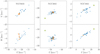 |
Fig. A.1. Example of (U, V, W) distribution of the member stars (blue) of the clusters NGC 6633, NGC 6281, and NGC 1662. Stars included in the spectroscopic analysis in this work are the orange crosses, and the stars discarded by discrepant kinematics are marked with green diamonds. The sample of member stars are those in Cantat-Gaudin et al. (2018) with membership probability > 0.7 and radial velocity determination in Gaia DR2. Not all plots are to the same scale. |
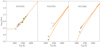 |
Fig. A.2. Example Teff − log g distribution of the spectroscopic targets (blue) of the clusters NGC 6705, NGC 6791, and NGC 2682. Isochrones of the corresponding age and metallicity of the cluster are overplotted, and the members discarded for being unlikely red clump stars are marked in green diamonds. |
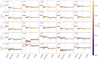 |
Fig. A.3. [X/H] solar-scaled abundances of all measured chemical species for all stars in the Hyades, NGC 3532, and IC 4756. Stars are colored and sorted by increasing Teff, and the size of the points is proportional to the log g. The solid black line indicates the mean abundance, and the colored band the standard deviation. For several elements (Zr, Ce, Pr) it was not possible to retrieve reliable values of abundance for the hottest stars. |
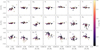 |
Fig. A.4. [X/Fe] abundances of all measured elements as a function of [Fe/H] colored by cluster age. |
All Tables
Median offsets and dispersions (MAD) found in Teff, log g, and [M/H] among stars observed with several instruments.
Details of the spectra of the observed stars identified by their Gaia DR2 source ID.
All Figures
|
Fig. 1. Uncertainties in the retrieved Teff (top) and log g (bottom) as a function of S/N. The colors show the computed log Teff. |
| In the text | |
|
Fig. 2. Number of clusters that have a given number of observed spectroscopic targets (blue), and those considered in our analysis as bona fide red clump stars. |
| In the text | |
|
Fig. 3. Top: X,Y distribution of the sample of OCs used in this work, where the Galactic center is towards the right. Bottom: Z, RGC distribution of the sample of clusters. The color represents the age of the cluster. The dashed lines indicate the position of the Sun (X⊙, Y⊙, Z⊙) = (0, 0, 0), RGC = 8.34 kpc. |
| In the text | |
|
Fig. 4. Gaia DR2 color-magnitude diagrams of the sample of clusters used (sorted by age), retained RC targets are marked with a blue cross. The gray points correspond to the membership selections by Cantat-Gaudin et al. (2018); Gaia Collaboration (2018a). PARSEC isochrones (Marigo et al. 2017) of the corresponding metallicity computed in this paper are overplotted using distances provided by CG20, and ages and extinctions detailed in Sect. 4. |
| In the text | |
|
Fig. 5. Teff–log g diagrams resulting from the analysis of the analyzed RC stars in blue. The clusters are sorted according to age. The same isochrones of Fig. 4 are overplotted with the corresponding [M/H] and age. |
| In the text | |
|
Fig. 6. Top: distribution of solar scaled iron abundances of all analyzed stars. Bottom: distribution of cluster ages as a function of mean [Fe/H] (clusters with one measured star are plotted in orange). |
| In the text | |
|
Fig. 7. Mean [Fe/H] values per cluster computed here (blue) compared with [M/H] literature values from Heiter et al. (2014) (orange) for the 23 clusters in common. |
| In the text | |
|
Fig. 8. Distribution of the uncertainties of abundances of the different elements: for the full sample of stars (blue), and the clusters with more than one measured star (orange). The median value is marked with a point, and the 16th and 84th percentiles are represented with the line. |
| In the text | |
|
Fig. 9. Gaia DR2 CMDs (gray dots) of the clusters for which the ages and extinctions were refined with respect to the ones in CG20, as discussed in the main text. The orange isochrones are those with the values quoted in CG20, and the green ones are manually changed to adjust the shape of the main sequence, turnoff or red giant members. Target stars studied in this paper are marked with blue crosses. |
| In the text | |
|
Fig. 10. [X/Fe] abundances of all measured elements as a function of age in logarithmic scale. Clusters located at less than 1 kpc from the Sun are plotted in orange. Uncertainties in the x coordinate are smaller than the points. Red circles correspond to the clusters with stars with more uncertain atmospheric parameters. |
| In the text | |
|
Fig. 11. Abundance ratios for which a significant level of correlation is found. Only clusters closer than 1 kpc and with more than one star are plotted. Error bars for the x-axis are usually smaller than the point size. The best-fit model is overplotted in black (the resulting slope written in each panel in dex Gyr−1), and the light gray lines correspond to the sampling of the MCMC. Element names are colored depending on the chemical family they belong to. |
| In the text | |
|
Fig. 12. [Y/Mg] (left) and [Y/Al] (right) abundances of our sample of clusters (with more than one measured star) as a function of age. In the top panel we plot the clusters closer than 1 kpc (orange), and in the bottom panel clusters at all distances. The clusters marked with red circles are those flagged in Sect. 2.4. The linear fits done for the close (all) clusters are plotted in orange (blue) lines, accounting for uncertainties. The values of the obtained slopes are indicated. The results of the linear fit performed by Spina et al. (2018) are shown in black for comparison purposes. |
| In the text | |
|
Fig. 13. Residuals in the [Y/Mg] (with respect to the linear fit for the closest sample Eq. (1)) versus age in three bins of Galactocentric radius, indicated in each panel. The color code is the derived [Fe/H] abundance. |
| In the text | |
|
Fig. A.1. Example of (U, V, W) distribution of the member stars (blue) of the clusters NGC 6633, NGC 6281, and NGC 1662. Stars included in the spectroscopic analysis in this work are the orange crosses, and the stars discarded by discrepant kinematics are marked with green diamonds. The sample of member stars are those in Cantat-Gaudin et al. (2018) with membership probability > 0.7 and radial velocity determination in Gaia DR2. Not all plots are to the same scale. |
| In the text | |
|
Fig. A.2. Example Teff − log g distribution of the spectroscopic targets (blue) of the clusters NGC 6705, NGC 6791, and NGC 2682. Isochrones of the corresponding age and metallicity of the cluster are overplotted, and the members discarded for being unlikely red clump stars are marked in green diamonds. |
| In the text | |
|
Fig. A.3. [X/H] solar-scaled abundances of all measured chemical species for all stars in the Hyades, NGC 3532, and IC 4756. Stars are colored and sorted by increasing Teff, and the size of the points is proportional to the log g. The solid black line indicates the mean abundance, and the colored band the standard deviation. For several elements (Zr, Ce, Pr) it was not possible to retrieve reliable values of abundance for the hottest stars. |
| In the text | |
|
Fig. A.4. [X/Fe] abundances of all measured elements as a function of [Fe/H] colored by cluster age. |
| In the text | |
Current usage metrics show cumulative count of Article Views (full-text article views including HTML views, PDF and ePub downloads, according to the available data) and Abstracts Views on Vision4Press platform.
Data correspond to usage on the plateform after 2015. The current usage metrics is available 48-96 hours after online publication and is updated daily on week days.
Initial download of the metrics may take a while.